3.1 Grid- and domain-sensitivity study

Figure 2.

Grid-sensitivity study with respect to (a) skin-friction coefficient and (b) wall-pressure evolution. Reported quantities are time and spanwise averaged. (- - - -) ${\mathcal{G}}^{1}$ , (– ⋅ – ⋅ –)  ${\mathcal{G}}_{z}^{1}$ , (——) ${\mathcal{G}}^{2}$ , (– $\cdot \cdot$ – $\cdot \cdot$ )  ${\mathcal{G}}_{x}^{2}$ , (● (grey)) ${\mathcal{G}}^{2}$ averaged over $446\unicode[STIX]{x1D6FF}_{0}/U_{0}$ , ( $\cdots \cdots$ ) inviscid interaction. The plateau pressure prediction according to Zukoski (Reference Zukoski1967) is also shown. See table 2 for reference.

A sensitivity study with respect to the chosen grid resolution as well as the spanwise domain extent is provided in the following. We start with the grid-sensitivity study for which table 2 summarises the main parameters. Figure 2(a,b) gives a comparison of time- and spanwise-averaged skin-friction coefficient $\langle C_{f}\rangle$ and wall-pressure evolution $\langle p_{w}\rangle /p_{\infty }$ . Comparing the coarsest grid resolution ${\mathcal{G}}^{1}$ ( $\unicode[STIX]{x0394}x^{+}=78$ , $\unicode[STIX]{x0394}y_{min}^{+}=0.9$ , $\unicode[STIX]{x0394}z^{+}=19.6$ ) with the next level ${\mathcal{G}}_{z}^{1}$ (refinement in spanwise direction) one can state that the overall wall-pressure evolution coincides, while larger deviations can be observed in the post-interaction region for the skin-friction coefficient. Mean separation and reattachment locations (defined through $\langle C_{f}\rangle =0$ ) and thus the resulting separation length $L_{sep}$ remain unaltered. Note that the pressure strongly decreases in the relaxation zone due to the influence of the PME, resulting in a significantly higher skin-friction level than for the incoming TBL. The inviscid wall-pressure evolution (dotted line in figure 2 a) clearly deviates from the stepwise pressure signal characteristic of a canonical inviscid shock reflection without PME. Characteristics emanating from the centred expansion in the current SWBLI already influence the incident shock (see shock curvature in figure 1), shifting the nominal inviscid shock impingement location downstream to $(x-x_{imp})/\unicode[STIX]{x1D6FF}_{0}=2.35$ . Note that the wall pressure in the post-interaction zone for $(x-x_{imp})/\unicode[STIX]{x1D6FF}_{0}>20$ asymptotically reaches the inviscid solution. The next grid level ${\mathcal{G}}^{2}$ differs from the previous one ${\mathcal{G}}_{z}^{1}$ in the number of cells in streamwise direction, resulting in a grid resolution of $\unicode[STIX]{x0394}x^{+}=39$ , $\unicode[STIX]{x0394}y_{min}^{+}=0.9$ and $\unicode[STIX]{x0394}z^{+}=9.8$ in streamwise, wall-normal and spanwise directions, respectively. A strong effect is found for the skin friction and wall pressure, which is related to a significant change in separation length (relative increase of $14.8\,\%$ compared to ${\mathcal{G}}_{z}^{1}$ ) and probably caused by the slightly different development of synthetic turbulence in the upstream TBL (see also the discussion related to Reynolds stresses in figure 4 b). Note that the location of reattachment remains the same, while the mean separation point moves upstream.

Having identified an influence on the results by the streamwise resolution, we doubled the number of cells in this direction, which results in grid configuration ${\mathcal{G}}_{x}^{2}$ ( $\unicode[STIX]{x0394}x^{+}=9.8$ ) with a total number of $727.3$ million cells. Both the mean wall pressure and skin friction now do not show significant changes any more. Note that we also include results on ${\mathcal{G}}^{2}$ for the same integration time of $446\unicode[STIX]{x1D6FF}_{0}/U_{0}$ as for the remaining grid resolutions (see grey bullets (●) in figure 2 a,b). The results suggest that the number of samples used in this study are sufficient to consider the results to be statistically converged with respect to the skin friction and wall pressure. Touber & Sandham (Reference Touber and Sandham2009) also investigated the sensitivity of their results to the grid resolution by refining the grid in each coordinate direction separately. They did not find significant dependencies of the size of the separation bubble with respect to the chosen grid resolution. While our results may imply a different conclusion it must be noted that their reference grid has a similar resolution expressed in wall units ( $\unicode[STIX]{x0394}x^{+}=40.6$ , $\unicode[STIX]{x0394}y_{min}^{+}=1.6$ , $\unicode[STIX]{x0394}z^{+}=13.5$ ) as our configuration ${\mathcal{G}}^{2}$ , for which we have identified that a further refinement does not change the overall results.

To further address the effect of grid resolution, we analyse the prediction of the plateau pressure by applying the free interaction concept. Carrière, Sirieix & Solignae (Reference Carrière, Sirieix and Solignae1969) report a generalised correlation function $\widetilde{{\mathcal{F}}}$ independent of Mach and Reynolds number. It accounts for non-uniformities in the incoming outer flow as well as for wall curvature effects and is especially suited for SWBLI featuring strong streamline curvature in the free interaction zone (Matheis & Hickel Reference Matheis and Hickel2015). While the pressure plateau value is around $\widetilde{{\mathcal{F}}}_{p}=6.4$ on ${\mathcal{G}}^{1}$ and ${\mathcal{G}}_{z}^{1}$ , we find a value of $\widetilde{{\mathcal{F}}}_{p}=6.0$ for the grid configurations ${\mathcal{G}}^{2}$ and ${\mathcal{G}}_{x}^{2}$ . The latter value is in perfect agreement with Erdos & Pallone (Reference Erdos and Pallone1963) who proposed a value of $6.0$ for the pressure plateau in turbulent flow. Figure 2(b) includes the plateau pressure prediction by Zukoski (Reference Zukoski1967). The prediction again matches the numerical results on grid levels ${\mathcal{G}}^{2}$ and ${\mathcal{G}}_{x}^{2}$ , suggesting that the Reynolds number in our studies ( $Re_{\unicode[STIX]{x1D6FF}_{0}}\approx 2\times 10^{5}$ ) is high enough such that the plateau pressure ratio essentially depends on the upstream Mach number.

Finally, we investigate the sensitivity of statistical results to the domain width. In total three configurations based on the grid resolution ${\mathcal{G}}^{2}$ have been considered. The reference span of $L_{z}=4.5\unicode[STIX]{x1D6FF}_{0}$ ( ${\mathcal{D}}^{2}$ ) is halved for ${\mathcal{D}}^{1}$ ( $L_{z}=2.25\unicode[STIX]{x1D6FF}_{0}$ ) and doubled for ${\mathcal{D}}^{3}$ ( $L_{z}=9\unicode[STIX]{x1D6FF}_{0}$ ), see table 3 for simulation parameters and figure 3 for corresponding results. While the small span LES ( ${\mathcal{D}}^{1}$ ) reveals a slightly smaller separation bubble (downstream and upstream shift of the separation and reattachment location, respectively) and a different skin-friction recovery, the results for the reference span ( ${\mathcal{D}}^{2}$ ) and the large span ( ${\mathcal{D}}^{3}$ ) are nearly undistinguishable.

Figure 3.

Domain-sensitivity study with respect to (a) skin-friction coefficient and (b) wall-pressure evolution. Reported quantities are time and spanwise averaged. (- - - -) ${\mathcal{D}}^{1}$ , (——)  ${\mathcal{D}}^{2}$ , (– ⋅ – ⋅ –) ${\mathcal{D}}^{3}$ . See table 3 for reference.

Figure 4.

(a) van Driest transformed mean velocity profile and (b) r.m.s. of Reynolds stresses with density scaling $\unicode[STIX]{x1D709}=\sqrt{\langle \unicode[STIX]{x1D70C}\rangle /\langle \unicode[STIX]{x1D70C}_{w}\rangle }$ for all grid resolutions at $Re_{\unicode[STIX]{x1D70F}}=1523$ and $(x-x_{imp})/\unicode[STIX]{x1D6FF}_{0}=-15.25$ : (- - - -)  ${\mathcal{G}}^{1}$ , (– ⋅ – ⋅ –) ${\mathcal{G}}_{z}^{1}$ , (——) ${\mathcal{G}}^{2}$ , (– $\cdot \cdot$ – $\cdot \cdot$ )  ${\mathcal{G}}_{x}^{2}$ . See table 2 for reference. ( $\odot$  (grey)) Incompressible DNS data adopted from Schlatter & Örlü (Reference Schlatter and Örlü2010) at $Re_{\unicode[STIX]{x1D70F}}=1271$ .

Figure 5.

Incompressible skin-friction distribution. (——) Present LES ( ${\mathcal{G}}^{2}$ ), (- - - -) Blasius, (– ⋅ – ⋅ –) Kármán–Schoenherr (both adopted from Hopkins & Inouye (Reference Hopkins and Inouye1971)), (– $\cdot \cdot$ – $\cdot \cdot$ ) Smits, Matheson & Joubert (Reference Smits, Matheson and Joubert1983), ( $\boxdot$ ) Pirozzoli & Bernardini (Reference Pirozzoli and Bernardini2011), ( $\odot$ ) Komminaho & Skote (Reference Komminaho and Skote2002), (▵) Schlatter & Örlü (Reference Schlatter and Örlü2010), (▿) Simens et al. (Reference Simens, Jiménez, Hoyas and Mizuno2009), ( $\unicode[STIX]{x2B20}$ ) Pirozzoli, Grasso & Gatski (Reference Pirozzoli, Grasso and Gatski2004),  $(\times )$ Maeder, Adams & Kleiser (Reference Maeder, Adams and Kleiser2001), ( $+$ ) Guarini et al. (Reference Guarini, Moser, Shariff and Wray2000), (♢) Coles (Reference Coles1953) (CAT5301, from Fernholz & Finley (Reference Fernholz and Finley1977)).

In figure 4, we report the van Driest transformed mean velocity profile as well as the r.m.s. of Reynolds stresses in Morkovin scaling for all grid resolutions and evaluated at the streamwise location $(x-x_{imp})/\unicode[STIX]{x1D6FF}_{0}=-15.25$ , which corresponds to a friction Reynolds number of $Re_{\unicode[STIX]{x1D70F}}=\unicode[STIX]{x1D70C}_{w}u_{\unicode[STIX]{x1D70F}}\unicode[STIX]{x1D6FF}/\unicode[STIX]{x1D707}_{w}=1523$ . The figure also includes incompressible DNS data of Schlatter & Örlü (Reference Schlatter and Örlü2010) at their highest available friction Reynolds number of $Re_{\unicode[STIX]{x1D70F}}=1271$ . The inner layer and log-law region are in good agreement with the logarithmic law of the wall (with $\unicode[STIX]{x1D705}=0.41$ and $C=5.2$ ) and the DNS data, with small differences recognisable in the wake region. The strength of the wake component increases with increasing momentum thickness Reynolds number and remains nearly constant above a value of approximately $6000$ (Coles Reference Coles1962; Smits & Dussauge Reference Smits and Dussauge2006; Gatski & Bonnet Reference Gatski and Bonnet2009). For the incompressible DNS data a momentum thickness Reynolds number of $4061$ is reported. In order to compare with incompressible data we compute $Re_{\unicode[STIX]{x1D703}_{i}}=(\unicode[STIX]{x1D707}_{0}/\unicode[STIX]{x1D707}_{w})Re_{\unicode[STIX]{x1D703}}=\unicode[STIX]{x1D70C}_{\infty }\unicode[STIX]{x1D703}U_{0}/\unicode[STIX]{x1D707}_{w}=6500$ , explaining the higher wake velocity observed in figure 4(a) for the present LES. The streamwise Reynolds stress on grid levels ${\mathcal{G}}^{1}$ and ${\mathcal{G}}_{z}^{1}$ , see figure 4(b), shows a significant overestimation of the peak value situated around $y^{+}\approx 10.5$ when compared to the DNS data. On grid level ${\mathcal{G}}^{2}$ the agreement with the reference data is very good, both in the inner and log layer. Further improvement within the log layer is obtained with ${\mathcal{G}}_{x}^{2}$ for the streamwise Reynolds stress. Note that the friction Reynolds number $Re_{\unicode[STIX]{x1D70F}}$ for the reference DNS is slightly lower, resulting in an earlier drop of the r.m.s. profiles at the wake region.

Finally we compare the skin-friction evolution obtained by the LES on grid level ${\mathcal{G}}^{2}$ with well-established correlations for incompressible flows, reference data from DNS and experimental data at different Mach numbers. A direct comparison with incompressible data is possible after applying the van Driest II transformation to the compressible results (van Driest Reference van Driest1956). Figure 5 shows the incompressible skin-friction coefficient $\langle C_{f_{i}}\rangle$ as a function of $Re_{\unicode[STIX]{x1D703}_{i}}$ . Our present LES results agree well with the incompressible relations of Smits et al. (Reference Smits, Matheson and Joubert1983), Blasius and Kármán–Schoenherr (both adopted from Hopkins & Inouye (Reference Hopkins and Inouye1971)), and available high Reynolds number data of Fernholz & Finley (Reference Fernholz and Finley1977).

The above grid- and domain-sensitivity studies have shown that the grid resolution ${\mathcal{G}}^{2}$ with a reference span of $L_{z}=4.5\unicode[STIX]{x1D6FF}_{0}$ properly resolves the incoming TBL and accurately predicts the interaction region. Small improvements of the streamwise Reynolds stress prediction within the log layer are possible by further increasing the streamwise grid resolution ( ${\mathcal{G}}_{x}^{2}$ ). However, the interaction region is unaffected by further refinement and thus we are confident that the grid resolution ${\mathcal{G}}^{2}$ is sufficiently fine. The analyses in the following are based on ${\mathcal{G}}^{2}$ .

3.2 Instantaneous and mean-flow organisation

Figure 6.

(a) Instantaneous contours of temperature in the $xy$ midplane together with isolines indicating mean (—— (black)) and instantaneous (—— (blue)) reversed flow. (b) Time- and spanwise-averaged contours of temperature. The shock system is visualised by isolines of pressure gradient magnitude $|\unicode[STIX]{x1D735}p|\unicode[STIX]{x1D6FF}_{0}/p_{\infty }=\{1.08,3.28\}$ . (—— (red))  $\langle \unicode[STIX]{x1D6FF}\rangle$ , (—— (black)) $\langle Ma\rangle =1$ , (—— (blue)) $\langle u\rangle =0$ .

A first impression of the flow field is provided in figure 6, where we show both instantaneous and mean contours of temperature. Isolines in figure 6(a) indicate the instantaneous and mean reversed flow (defined through $u/u_{\infty }=0$ and $\langle u\rangle /u_{\infty }=0$ , respectively). Additional isolines in figure 6(b) represent the shock system, the sonic line and the boundary-layer edge, where the latter is defined through an isovalue of mean spanwise vorticity $\langle \unicode[STIX]{x1D714}_{z}\rangle$ that gives the same boundary-layer thickness as the velocity-valued definition upstream of the interaction. Clearly, the adverse pressure gradient imposed by the incident shock is strong enough to cause a large flow separation and a separation shock originating well ahead of the inviscid impingement location. Note that $x_{imp}$ is related to the theoretical location at which a straight incident shock would impinge on the flat plate in the absence of a centred PME, thus neglecting shock curvature effects. The separation shock intersects the incident shock well outside the TBL, indicating the strong character of the interaction. Délery & Marvin (Reference Délery and Marvin1986) further characterised a strong interaction through the presence of three inflection points in the wall-pressure evolution, which are associated with the separation, the onset of reattachment and the reattachment compression. For even stronger interactions with an extended separated flow, a noticeable pressure plateau develops, as is the case for the present study (see figure 2 b,c). The separation-shock foot penetrates deeply into the incoming TBL, a phenomenon associated with the high Reynolds number of the flow (Loginov, Adams & Zheltovodov Reference Loginov, Adams and Zheltovodov2006; Ringuette et al. Reference Ringuette, Bookey, Wyckham and Smits2009). As will be discussed later in § 3.3, this feature causes a stronger footprint on the fluctuating wall-pressure signal as compared to SWBLI at lower Reynolds number and same Mach number (Adams Reference Adams2000; Pasquariello et al. Reference Pasquariello, Grilli, Hickel and Adams2014; Nichols et al. Reference Nichols, Larsson, Bernardini and Pirozzoli2016). In the same figure the formation of a detached turbulent shear layer originating from the separation shock is visible and contains the separated-flow area. Compression waves are formed along with the reattachment process, which finally coalesce into the reattachment shock. The instantaneous separation bubble is strongly perturbed near the initial part of the interaction zone, probably being related to fluid entrainment through the shear-layer vortices in this region (Piponniau et al. Reference Piponniau, Dussauge, Debiève and Dupont2009). The TBL grows significantly across the interaction, reaching a maximum of approximately $3\unicode[STIX]{x1D6FF}_{0}$ in the vicinity of the separation-bubble apex, see figure 6(b). The subsequent PME reduces the TBL thickness, which settles down to a value of $2\unicode[STIX]{x1D6FF}_{0}$ downstream of the interaction.

Figure 7.

(a) Skin-friction and (b) wall-pressure evolution: (——) present LES (averaged in time and spanwise direction; spanwise minimum and maximum values of the time-averaged data are indicated by the grey shaded area for the long integration time of $3805\unicode[STIX]{x1D6FF}_{0}/U_{0}$ and by dots for the short integration time of $446\unicode[STIX]{x1D6FF}_{0}/U_{0}$ ), (●) experimental static pressure measurements and ( $\unicode[STIX]{x2B20}$ ) mean experimental unsteady pressure measurements from Daub et al. (Reference Daub, Willems and Gülhan2015). Error bar indications are only approximate experimental estimates due to Willems (Reference Willems2016).

The mean separation length is determined from the skin-friction distribution shown in figure 7(a) and results in $L_{sep}=15.5\unicode[STIX]{x1D6FF}_{0}$ . Mean separation $x_{s}$ and reattachment $x_{r}$ locations are indicated by vertical dashed lines and are located at $(x-x_{imp})/\unicode[STIX]{x1D6FF}_{0}=-11.25\unicode[STIX]{x1D6FF}_{0}$ and $4.25\unicode[STIX]{x1D6FF}_{0}$ , respectively. Priebe & Martín (Reference Priebe and Martín2012) found in their compression corner results that the separation is not uniformly strong in the sense that the skin-friction coefficient varies within the separated-flow region. More precisely, their skin-friction distribution (see figure 4(a) in their publication) reveals a less strong separated flow approximately $1/3L_{sep}$ downstream of the mean separation location, resulting in a local $\langle C_{f}\rangle$ maximum. They related this behaviour to collapse events of the separation bubble during the low-frequency unsteadiness and found a positive skin-friction coefficient in this region for conditional averages of collapsing bubbles. Our results, however, show a rather uniformly strong separation over a streamwise length of approximately $2/3L_{sep}$ , which is probably related to the intensity of the present SWBLI. The pressure distribution reported in Priebe & Martín (Reference Priebe and Martín2012) does not exhibit a pressure plateau and the overall separation length of $3\unicode[STIX]{x1D6FF}_{0}$ is considerably smaller compared to our results. Furthermore, Clemens & Narayanaswamy (Reference Clemens and Narayanaswamy2014) have shown by a simple scaling analysis that the upstream momentum fluctuations may be large enough to provoke a bubble collapse in case of weakly separated flows but not for strong separations.

The grey shaded area in figure 7(a) indicates three-dimensional structures in the nominally two-dimensional interaction by considering spanwise minimum and maximum values of the time-averaged data $(3805\unicode[STIX]{x1D6FF}_{0}/U_{0})$ . In the incoming TBL, a very low spanwise variation of $\langle C_{f}\rangle$ is found, indicating statistical convergence. Two regions can be identified where evidence of stationary or slowly evolving three-dimensional flow structures exists: in the proximity of the mean separation location at $-11.25<(x-x_{imp})/\unicode[STIX]{x1D6FF}_{0}<-7.5$ and downstream of the inviscid impingement location at $(x-x_{imp})/\unicode[STIX]{x1D6FF}_{0}>0$ . Note that we also include results of the short duration LES (the dotted lines correspond to an integration time of $446\unicode[STIX]{x1D6FF}_{0}/U_{0}$ ). Our results imply that a significant spanwise modulation of the flow is present close to the separation and reattachment location. The underlying flow structures provoking this variation are unsteady in nature, as the time-averaged spanwise minimum and maximum values reduce with longer integration times. Time scales associated with such flow phenomena are considerably longer than the characteristic time scale of the incoming TBL ( $\unicode[STIX]{x1D6FF}_{0}/U_{0}$ ), since spanwise variations are still visible for the long-duration LES close to the separation and reattachment locations but vanish upstream of the interaction. We will provide support for this assumption in the course of this section and later in § 3.4.

A similar analysis has been conducted by Loginov et al. (Reference Loginov, Adams and Zheltovodov2006) for their LES of a compression corner flow. Their results cover an integration time of $703\unicode[STIX]{x1D6FF}_{0}/U_{0}$ , possibly explaining the strong spanwise variation of $\pm 2.4\times 10^{-4}$ found in their incoming TBL. Note that our short time LES shows a significantly lower variation of $\pm 5.0\times 10^{-5}$ . They found two pairs of possibly steady counter-rotating streamwise vortices originating in the proximity of the compression corner and termed them Görtler-like vortices, bearing similarities with the instability mechanism found experimentally for laminar boundary layers developing on sufficiently concave surfaces (Görtler Reference Görtler1941; Floryan Reference Floryan1991). We will resume this discussion later in this section and show that a similar mechanism exists for the current SWBLI. Figure 7(b) shows the wall-pressure distribution for both LES and experiment. Similar to the findings of Loginov et al. (Reference Loginov, Adams and Zheltovodov2006), a less strong spanwise variation is observed for the wall pressure. Experimental uncertainties have been estimated taking into account the accuracy of the sensors, uncertainties in wind tunnel flow conditions (total pressure, Mach number) and geometric uncertainties (alignment of the shock generator and the baseplate), see Willems (Reference Willems2016). Both datasets are in good agreement, with a relative error with respect to the maximum pressure of $\langle p_{max,LES}\rangle /\langle p_{max,exp}\rangle -1=-0.029$ . For demonstration, the mean wall pressure obtained through unsteady pressure measurements is shown for an upstream position and close to the separation location.

Figure 8.

Time- and spanwise-averaged Reynolds normal stress components. The shock system is visualised by isolines of pressure gradient magnitude $|\unicode[STIX]{x1D735}p|\unicode[STIX]{x1D6FF}_{0}/p_{\infty }=\{1.08,3.28\}$ . (—— (red)) $\langle \unicode[STIX]{x1D6FF}\rangle$ , (—— (black)) $\langle Ma\rangle =1$ , (—— (blue)) $\langle u\rangle =0$ , (—— (grey)) dividing streamline $y_{ds}$ . A star ( $\star$ ) indicates the location of maximum contour level. Eight discrete contour levels are shown by dashed lines.

The effect of the SWBLI on the normal Reynolds stress components is analysed in figure 8. In each figure, we again indicate the shock system, boundary-layer thickness, sonic line and reverse flow region by individual isolines. Additionally, the grey isoline indicates the dividing streamline defined by the set of points $y_{ds}(x)$ for which $\int _{0}^{y_{ds}}\langle \unicode[STIX]{x1D70C}u\rangle \,\text{d}y=0$ . The region of highest Reynolds stress is indicated by a star and eight contour levels are superimposed by dashed lines. A high level of streamwise Reynolds stress $\langle u^{\prime }u^{\prime }\rangle$ is found along the detached shear layer with its maximum located at the separation-shock foot, see figure 8(a). The strong convex streamline curvature near the bubble apex considerably damps the Reynolds stresses (see Smits & Dussauge Reference Smits and Dussauge2006, e.g.). A similar observation was made by Sandham (Reference Sandham2016). A second branch of increased $\langle u^{\prime }u^{\prime }\rangle$ is found in the proximity of the reattachment location but located farther away from the wall. Shear-layer vortices in this region are convected downstream with the flow and interact with the reattachment compression, possibly explaining this local maximum of streamwise Reynolds stress. For the wall-normal Reynolds stress component $\langle v^{\prime }v^{\prime }\rangle$ , see figure 8(b), increased levels are found along the separation and reattachment shocks and are directly associated with their unsteady motion. The spanwise Reynolds stress component $\langle w^{\prime }w^{\prime }\rangle$ shares some similarities with the streamwise component, but one remarkable difference is observed: in the proximity of reattachment, where the dividing streamline shows a high level of concave curvature, another area of increased Reynolds stress is observed with its maximum located approximately $3\unicode[STIX]{x1D6FF}_{0}$ downstream and attached to the wall. This region of increased spanwise Reynolds stress covers $3.5<(x-x_{imp})/\unicode[STIX]{x1D6FF}_{0}<12.5$ . To the authors’ knowledge, no such phenomenon has been previously reported for impinging SWBLI. Similarities with the compression corner results of Loginov et al. (Reference Loginov, Adams and Zheltovodov2006) discussed previously suggest that a similar centrifugal instability plays a role for the current SWBLI, which would explain the increased spanwise Reynolds stress found in figure 8(c). Furthermore, the PME centred at the bubble apex, the dividing streamline and the downstream recompression correspond to a two-dimensional supersonic backward-facing step flow, for which streamwise vortices have been found experimentally in laminar, transitional and turbulent flows over a large range of Mach numbers (Ginoux Reference Ginoux1971).

Figure 9.

Instantaneous visualisation of the reversed flow and the Görtler-like vortices at two uncorrelated times. Translucent isosurface of streamwise velocity $u=0$ (blue) and isosurfaces of streamwise vorticity $\unicode[STIX]{x1D714}_{x}=\pm 0.4U_{0}/\unicode[STIX]{x1D6FF}_{0}$ (white/black) are shown.

Figure 10.

Numerical oil paint imitation together with mean skin-friction contours. Thick solid lines indicate time-averaged separation and reattachment locations defined by $\langle C_{f}\rangle =0$ . Contour cutoff level is $\langle C_{f}\rangle =2\times 10^{-3}$ . Time integration covers (a) $446\unicode[STIX]{x1D6FF}_{0}/U_{0}$ and (b) $3805\unicode[STIX]{x1D6FF}_{0}/U_{0}$ .

In figure 9, we show the instantaneous structure of the flow at two uncorrelated time instants. The blue isosurface indicates the reverse flow region ( $u=0$ ), while the white and black isosurfaces correspond to a positive and negative value of streamwise vorticity ( $\unicode[STIX]{x1D714}_{x}=\pm 0.4U_{0}/\unicode[STIX]{x1D6FF}_{0}$ ). As other authors have already pointed out (Loginov et al. Reference Loginov, Adams and Zheltovodov2006; Grilli et al. Reference Grilli, Hickel and Adams2013), the circulation of the Görtler-like vortices found in compression corner studies is rather small, which makes it difficult to extract them from background turbulent structures. For visualisation purposes we apply both a temporal and spatial filter on three-dimensional snapshots of the flow. Temporal filtering is accomplished by a simple moving-average filter. Although the roll-off capabilities and the frequency response for such a filter are very poor, the noise suppression in the time domain is excellent. The LES database consists of $n_{s}=7614$ three-dimensional snapshots recorded at a sampling interval of $\unicode[STIX]{x0394}t_{s}=0.5\unicode[STIX]{x1D6FF}_{0}/U_{0}$ . We select a filter width of $n_{f}=51$ snapshots for the moving-average frame. Subsequently, a top-hat filter is applied to the temporally averaged data with a constant filter width in streamwise and spanwise direction equal to $\unicode[STIX]{x0394}x_{f}=0.22\unicode[STIX]{x1D6FF}_{0}$ and $\unicode[STIX]{x0394}z_{f}=0.07\unicode[STIX]{x1D6FF}_{0}$ , while in wall-normal direction the filter width is spanned by four computational cells.

The following qualitative observations can be made from figure 9(a,b): two pairs of counter-rotating streamwise vortices develop in the reattachment region. These Görtler-like vortices are not fixed at a specific spanwise position, contrary to the results of Loginov et al. (Reference Loginov, Adams and Zheltovodov2006). Note that the inflow boundary condition in their LES contained low-amplitude steady structures, which may lock the spanwise position of the streamwise vortices, similar to model imperfections in experimental configurations (Floryan Reference Floryan1991). Another aspect is their short integration time, which might not capture low-frequency modulations of such flow structures. In accordance with experimental observations (Görtler Reference Görtler1941; Floryan Reference Floryan1991; Schülein & Trofimov Reference Schülein and Trofimov2011) as well as numerical findings (Loginov et al. Reference Loginov, Adams and Zheltovodov2006; Grilli et al. Reference Grilli, Hickel and Adams2013), the spanwise width of each vortex pair is approximately $2\unicode[STIX]{x1D6FF}_{0}$ . The spanwise width of our computational domain of $L_{z}=4.5\unicode[STIX]{x1D6FF}_{0}$ in combination with periodic boundary conditions allow flow structures with a spanwise wavelength of at most $4.5\unicode[STIX]{x1D6FF}_{0}$ to be captured. We investigated the wavelength on our large-span configuration ${\mathcal{D}}^{3}$ with $L_{z}=9\unicode[STIX]{x1D6FF}_{0}$ and found the same width of about $2\unicode[STIX]{x1D6FF}_{0}$ for a vortex pair. The effect of the streamwise vortices on the separated flow is clearly visible in figure 9(b): vortex-induced upwash decreases the shear stress at this specific spanwise location and directly influences the reattachment position by shifting it further downstream. Indeed, at $z/\unicode[STIX]{x1D6FF}_{0}\approx -0.4$ such a flow configuration can be observed. Vortex-induced downwash ( $z/\unicode[STIX]{x1D6FF}_{0}\approx 1$ ) increases the local shear stress and subsequently shifts the reattachment position further upstream. The above findings suggest a direct coupling between the separated-flow dynamics and the streamwise vortices. As pointed out by Floryan (Reference Floryan1991), such vortices in turbulent flow have no spanwise preference position and thus meander in time. Steady non-uniformities, e.g. when small vortex generators are placed in the settling chamber of a wind tunnel, might induce a preferred lateral position around which the spanwise motion occurs. In case that the level of unsteady disturbances of the oncoming flow is large compared to that of the steady disturbances, however, no preferred spanwise position can be observed for Görtler-like vortices (Kottke Reference Kottke1988; Floryan Reference Floryan1991). An animation of figure 9 reveals that the streamwise vortices tend to meander in the lateral direction. At the same time the vortices appear and disappear, coalesce and separate in an apparently random manner. Consequently, the effect of the Görtler-like vortices on the mean spanwise flow modulation diminishes with increasing averaging time. This is also evident when looking at figure 10, where we show a numerical oil flow visualisation together with mean skin-friction contours evaluated for the wall plane. While figure 10(a) is obtained for the short-duration LES, figure 10(b) includes a large number of low-frequency oscillations of the separation bubble. Characteristic node and saddle points close to the reattachment location can be observed for the former. Convergence and divergence lines associated with regions of vortex-induced upwash and downwash indicate a strong spanwise modulation of the flow for the time frame considered. While figure 10(a) might suggest a system of steady streamwise vortices to be present, the results for the long-run LES clearly suggest the streamwise vortices to be unsteady. Node and saddle points as well as convergence and divergence lines appear suppressed in figure 10(b), indicating a less strong spanwise modulation of the mean flow with increasing averaging time.

Figure 11.

(a) Curvature parameter $\unicode[STIX]{x1D6FF}/R$ and (b) Görtler number $G_{T}$ evaluated along a mean-flow streamline passing through $(x-x_{imp})/\unicode[STIX]{x1D6FF}_{0}=-15$ and $y/\unicode[STIX]{x1D6FF}_{0}=0.75$ . (- - - -) stability limits according to Görtler (Reference Görtler1941) and Smits & Dussauge (Reference Smits and Dussauge2006).

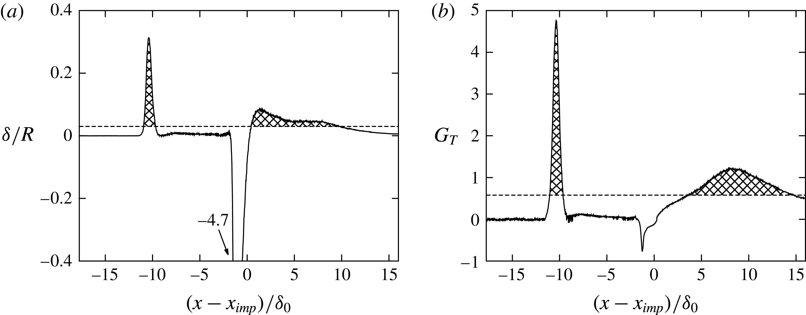
Figure 11 analyses the curvature parameter $\unicode[STIX]{x1D6FF}/R$ and the Görtler number $G_{T}$ for a mean-flow streamline passing through $(x-x_{imp})/\unicode[STIX]{x1D6FF}_{0}=-15$ and $y/\unicode[STIX]{x1D6FF}_{0}=0.75$ . According to Loginov et al. (Reference Loginov, Adams and Zheltovodov2006) and Smits & Dussauge (Reference Smits and Dussauge2006), the Görtler number for a compressible turbulent flow may be defined as

Therein $\unicode[STIX]{x1D6FF}_{1}$ , $\unicode[STIX]{x1D703}$ and $R$ denote the displacement thickness, the momentum thickness and the streamline curvature radius of the mean flow, respectively. Note that we have modified the above expression to indicate convex and concave curvature. Smits & Dussauge (Reference Smits and Dussauge2006) report a lower limit for the curvature parameter above which longitudinal vortices are expected to develop, this being $\unicode[STIX]{x1D6FF}/R\approx 0.03$ for a $Ma=3$ flow. In laminar flow the critical Görtler number is $G_{T}=0.58$ (Görtler Reference Görtler1941). Both limits are significantly exceeded within a short region close to the separation point as well as within a long region at reattachment (see filled patterns in figure 11(a,b). Although it is unclear whether such stability criteria hold also for turbulent flow, the high values within the reattachment region, which last over a significantly long streamwise distance of $11\unicode[STIX]{x1D6FF}_{0}$ , indicate a centrifugal instability to be a plausible mechanism for the generation of Görtler-like vortices.

3.3 Spectral analysis

Figure 12.

(a) Numerical and (b) experimental wall-pressure signal near the separation-shock foot. The numerical probe is located at mean separation $x_{s}$ , low-pass filtered with a finite impulse rate filter (cutoff Strouhal number of $St_{\unicode[STIX]{x1D6FF}}=0.33$ , filter order of $900$ ) and subsequently projected on the experimental time axis via linear interpolation. Locations of the experimental and numerical pressure probe are indicated in figure 7. (c) Weighted power spectral density $f\cdot {\mathcal{P}}(f)$ for the raw pressure signals without low-pass filtering. Experimental data from Daub et al. (Reference Daub, Willems and Gülhan2015) with (—— (grey)) $T_{seg}=374L_{sep}/U_{0}$ ( $n_{seg}=130$ ) and (- - - - (grey)) $T_{seg}=51L_{sep}/U_{0}$ ( $n_{seg}=973$ ). (——) LES with $T_{seg}=51L_{sep}/U_{0}$ ( $n_{seg}=12$ ).

The unsteadiness of the present SWBLI is studied in this section by means of spectral analysis. For this purpose, $1230$ equally spaced wall-pressure probes have been placed in streamwise direction along the midplane of the computational domain. The probes span the region $-17.74<(x-x_{imp})/\unicode[STIX]{x1D6FF}_{0}<17.18$ and are sampled at a frequency of approximately $f_{s}=60U_{0}/\unicode[STIX]{x1D6FF}_{0}$ , which corresponds to $8.9~\text{MHz}$ . Figure 12(a,b) compares a section of the experimental wall-pressure measurement (Daub et al. Reference Daub, Willems and Gülhan2015) with the LES signal. Both signals have been evaluated near the separation-shock foot, i.e. the experimental location is given by the unsteady pressure transducer indicated in figure 7(b), whereas the LES signal has been extracted at the mean separation location $x_{s}$ . As mentioned in § 2.2, the cutoff frequency of the experimental measurements is $50~\text{kHz}(0.33U_{0}/\unicode[STIX]{x1D6FF}_{0})$ . Consequently, scales in the incoming TBL, whose characteristic frequency is of the order of $U_{0}/\unicode[STIX]{x1D6FF}_{0}$ , are undersampled. In order to mimic the experimental cutoff effect, we low-pass filter the LES signal with a finite impulse rate (FIR) filter of order $900$ and a $-6~\text{dB}$ cutoff Strouhal number of $St_{\unicode[STIX]{x1D6FF}}=0.33$ . Subsequently, the filtered signal is projected on the experimental time axis via linear interpolation. Qualitative similarities between both datasets can be observed in terms of intermittency, occurring time scales and wall-pressure amplitudes. In contrast to previous low Reynolds numerical studies (Adams Reference Adams2000; Touber & Sandham Reference Touber and Sandham2009; Priebe & Martín Reference Priebe and Martín2012; Pasquariello et al. Reference Pasquariello, Grilli, Hickel and Adams2014), our filtered signal shows the well-known intermittent character typically observed in high Reynolds number experiments, that is, the wall-pressure jumps from the incoming TBL value to that behind the separation shock and back again. This effect is attributed to the high Reynolds number of the flow as shown experimentally by Dolling & Murphy (Reference Dolling and Murphy1983) and Dolling & Or (Reference Dolling and Or1985). At lower Reynolds number the separation shock does not penetrate as far into the TBL as it does at high Reynolds number. In fact, the separation shock is diffused by increased viscous effects when approaching the wall. Since its motion is no longer associated with a single, well-defined shock wave, its intermittency is attenuated (Adams Reference Adams2000; Ringuette et al. Reference Ringuette, Bookey, Wyckham and Smits2009).

A more quantitative comparison of both signals is given in figure 12(c), where we show the weighted power spectral density (PSD) of the two signals. Note that the LES signal is not low-pass filtered for this comparison, thus retaining the high-frequency TBL content. Welch’s algorithm with Hamming windows is used to estimate the PSD. For the LES signal (black solid line), a total number of $n_{seg}=12$ segments is used with $65\,\%$ overlap. These parameters lead to a segment length of approximately $783\unicode[STIX]{x1D6FF}_{0}/U_{0}(51L_{sep}/U_{0})$ . For the available experimental signal two segmentation configurations have been used. The grey solid line reflects a total number of $n_{seg}=130$ segments with $65\,\%$ overlap. This leads to an individual window length of $5797\unicode[STIX]{x1D6FF}_{0}/U_{0}(374L_{sep}/U_{0})$ and should resolve all expected low-frequency dynamics properly. The parameters for the grey dashed line are chosen in such a way that the individual segment length is the same as for the LES, leading to a total number of $n_{seg}=973$ segments. The good qualitative agreement between both signals observed in figure 12(a,b) is also confirmed by their spectra. Both spectra indicate the presence of a dominant low-frequency peak around a non-dimensional frequency of $St_{L_{sep}}=fL_{sep}/U_{0}\approx 0.04$ . This value agrees well with experimental studies for different flow geometries and upstream conditions by Dussauge, Dupont & Debiève (Reference Dussauge, Dupont and Debiève2006), who found that the unsteadiness occurs at frequencies centred about $St_{L_{sep}}=0.02{-}0.05$ . While the peak amplitude for the shock unsteadiness is captured very well by the LES, we observe a lower energy level for frequencies below the low-frequency peak. We have computed the PSD for a reduced number of segments $n_{seg}$ in order to allow for increased low-frequency resolution. We find that the energy content of the LES signal at frequencies below $St_{L_{sep}}<0.04$ essentially is unaffected. We believe that the observed discrepancies may be caused by side wall effects in the experiment which mainly show up at low frequencies. The LES data show an additional bump centred around $f\unicode[STIX]{x1D6FF}_{0}/U_{0}\approx 1$ , associated with the most energetic scales of the TBL. The experimental cutoff frequency of $0.33U_{0}/\unicode[STIX]{x1D6FF}_{0}$ excludes this range from the experimental data.

Figure 13.

Weighted power spectral density map. At each streamwise location the weighted spectra are normalised by $\int {\mathcal{P}}(f)\,\text{d}f$ . Mean separation and reattachment locations are highlighted by vertical dashed lines.

The wall-pressure spectrum for all numerical probes is shown in figure 13. Mean separation and reattachment locations are indicated by vertical dashed lines. Note that no energetically significant low-frequency content is apparent in the upstream TBL, proving the suitability of the digital filter technique. In accordance with previous numerical (Touber & Sandham Reference Touber and Sandham2009; Priebe & Martín Reference Priebe and Martín2012; Grilli et al. Reference Grilli, Schmid, Hickel and Adams2012) and experimental (Thomas et al. Reference Thomas, Putnam and Chu1994; Dupont et al. Reference Dupont, Haddad and Debiève2006) studies, the broadband peak associated with energetic scales in the incoming TBL shifts towards significantly lower frequencies close to the mean separation location and moves back again to higher frequencies downstream of the interaction. Within the rear part of the separation bubble so-called medium frequencies around $St_{L_{sep}}\approx 0.5$ develop, which are probably related to shear-layer vortices convected over the recirculation (Dupont et al. Reference Dupont, Haddad and Debiève2006). While the low-frequency activity is concentrated around the mean separation location, another significant level of unsteadiness is found slightly upstream and at frequencies around $0.1U_{0}/L_{sep}$ . Associated time scales of approximately $10L_{sep}/U_{0}$ can be found in the wall-pressure signal, see figure 12(a,b), and are related to the intermittent character of the separation shock as will be shown in figure 15.

The streamwise variation in r.m.s. wall-pressure fluctuations is shown in figure 14. The distributions are obtained by integrating the power spectra over a given frequency range

We focus on the low-frequency contributions of pressure fluctuations and thus select $f_{2}=1U_{0}/L_{sep}$ , see also figure 12(c). At the same time this value is sufficiently far away from the experimental cutoff frequency of $5.2U_{0}/L_{sep}$ , hence avoiding aliasing effects. The lower limit $f_{1}$ is chosen to be the smallest resolved frequency, individually selected for experiment (filled bullets) and LES (solid line). The overall agreement within the separated-flow region and after reattachment is satisfactory, while the peak value associated with the separation shock motion is underestimated by the LES. This effect can be attributed to the longer sampling time for the experiment, thus resolving much lower frequencies that contribute to the overall energy level. In fact, when restricting the integration of the experimental data to the same lower value $f_{1}$ as for the LES (open symbols in figure 14 a), the peak r.m.s. value reproduces the numerical result without affecting the other measurement locations.

Figure 14.

(a) Band-limited root mean square of wall-pressure fluctuations. (——) LES data obtained by integrating the PSD for $St_{L_{sep}}<1$ , (●) experimental data from Daub et al. (Reference Daub, Willems and Gülhan2015) obtained by integrating the PSD for $St_{L_{sep}}<1$ and ( $\unicode[STIX]{x2B20}$ ) by integrating the PSD for $0.014<St_{L_{sep}}<1$ . (b) Band-limited ( $St_{L_{sep}}<1$ ) relative root mean square of wall-pressure fluctuations for the present LES. (▴) indicate locations which will be discussed in conjunction with figure 15.

Similarly to experimental observations (Dolling & Murphy Reference Dolling and Murphy1983; Dolling & Or Reference Dolling and Or1985; Selig et al. Reference Selig, Andreopoulos, Muck, Dussauge and Smits1989), the high Reynolds number of the flow leads to a distinct r.m.s. peak centred around $x_{s}$ . Directly downstream a plateau region develops, followed by a continuous increase in pressure fluctuations until a second maximum is reached. Note that the second maximum is located $2.4\unicode[STIX]{x1D6FF}_{0}$ downstream of the mean reattachment location. This position apparently coincides with the reattaching shear layer, see figure 6(a), for which a characteristic frequency of the reattaching large-scale vortices is usually found around $0.5U_{0}/L_{sep}$ (Dupont et al. Reference Dupont, Haddad and Debiève2006). In figure 14(b) we further investigate the band-limited low-frequency contribution of pressure fluctuations to the total fluctuation energy for the present LES. In the incoming TBL approximately $10\,\%$ of the total r.m.s. of wall-pressure fluctuations reside in the lower-frequency range of $f<1U_{0}/L_{sep}$ . A similar value has been found experimentally by Thomas et al. (Reference Thomas, Putnam and Chu1994). When approaching the mean separation point, almost the complete ( $95\,\%$ ) pressure-fluctuation intensity is associated with such low frequencies. Thomas et al. (Reference Thomas, Putnam and Chu1994) investigated experimentally a compression corner flow at a free stream Mach number of $1.5$ and a Reynolds number of $Re_{\unicode[STIX]{x1D6FF}}\approx 178\times 10^{3}$ . They found that the fraction of fluctuation intensity that is associated with separation-shock oscillation increases with increasing ramp angle. For their largest ramp angle of $12^{\circ }$ a ratio of $55\,\%$ is reported, which is significantly lower than our value and possibly related to the considerably lower Mach number and weaker interaction in their study. Close to reattachment the low-frequency contribution is still responsible for $55\,\%$ of the total wall-pressure-fluctuation intensity and composed of a superposition of separation-bubble dynamics and reattaching shear-layer vortices convected downstream.

Figure 15.

Wall-pressure signals (a) and corresponding normalised probability density distributions (b) evaluated at $(x-x_{imp})/\unicode[STIX]{x1D6FF}_{0}=\{-17.74,-11.66,-11.34,4.25,6.61,17.18\}$ . Refer to the text and figure 14 for a physical interpretation of the wall-pressure positions. The mean wall pressure is indicated by a horizontal dashed line. Arrows together with vertical bars indicate the mean wall pressure and its standard deviation. Values of skewness $\unicode[STIX]{x1D6FC}_{3}$ and flatness $\unicode[STIX]{x1D6FC}_{4}$ coefficients and a Gaussian distribution are included for reference.

Figure 16.

(a) Streamwise intermittency distribution $\unicode[STIX]{x1D6FE}_{i}(x)$ . The mean separation location $x_{s}$ is indicated. ( $\unicode[STIX]{x2B20}$ ) highlight $1\,\%$ and $99\,\%$ intermittency boundaries and define the intermittent length scale $L_{i}=1.2\unicode[STIX]{x1D6FF}_{0}$ . (b) Skewness coefficient $\unicode[STIX]{x1D6FC}_{3}$ as a function of intermittency $\unicode[STIX]{x1D6FE}_{i}$ . (——) LES. Symbols represent experimental data from Dolling & Or (Reference Dolling and Or1985) for a compression ramp flow at a Mach number of $Ma=2.9$ and a Reynolds number of $Re_{\unicode[STIX]{x1D6FF}_{0}}=1.43\times 10^{6}$ with wedge angles ( $\blacklozenge$ )  $\unicode[STIX]{x1D717}=12^{\circ }$ (attached flow), (●) $\unicode[STIX]{x1D717}=16^{\circ }$ (incipient separation), (▴) $\unicode[STIX]{x1D717}=20^{\circ }$ (separated flow) and (▪) $\unicode[STIX]{x1D717}=24^{\circ }$ (separated flow).

The intermittent character of the wall pressure is further analysed in figure 15. On the left we show the normalised wall-pressure evolution for six different streamwise locations. On the right the corresponding normalised probability density functions (PDFs) computed from $228\,681$ samples grouped into $478$ bins, together with a standard Gaussian distribution are shown. The individual positions are indicated in the r.m.s. plot of wall-pressure fluctuations, see figure 14. From top to bottom they refer to the undisturbed TBL, the onset of interaction, the location of maximum wall-pressure fluctuation intensity, the mean reattachment position, the reattaching shear layer and the post-interaction location. The incoming TBL signal is effectively Gaussian, which is also reflected by the skewness $\unicode[STIX]{x1D6FC}_{3}$ and flatness $\unicode[STIX]{x1D6FC}_{4}$ coefficients.

The next probe is located $0.41\unicode[STIX]{x1D6FF}_{0}$ upstream of the mean separation location at a pressure level of $\langle p_{w}\rangle /\langle p_{w,0}\rangle =1.07$ . The signal is strongly intermittent. This is also confirmed by the associated PDF which is highly skewed and has a single mode at $-0.5\unicode[STIX]{x1D70E}_{p_{w}}$ , thus reflecting the probability of finding pressures in the range of the incoming TBL. Close to the mean separation location, at a pressure level of $\langle p_{w}\rangle /\langle p_{w,0}\rangle =1.27$ , the signal is still intermittent. Its PDF is highly left skewed with tendencies to develop a bimodal shape whose centres are located around $\pm 1\unicode[STIX]{x1D70E}_{p_{w}}$ . These two pressure probes have been evaluated at a very similar pressure ratio as done by Dolling & Murphy (Reference Dolling and Murphy1983). The reported wall-pressure signals and PDF qualitatively agree with experimental observations by Dolling & Murphy (Reference Dolling and Murphy1983) (see figure 6 in the respective publication) and Dolling & Or (Reference Dolling and Or1985) (see figure 3 in their publication), which again confirms the high Reynolds number character of the present SWBLI. The bimodal character is more pronounced in their studies, which is probably because of the even higher Reynolds number of $Re_{\unicode[STIX]{x1D6FF}_{0}}=1.43\times 10^{6}$ in their experiment. At the mean reattachment position the signal is slightly left skewed, see also Adams (Reference Adams2000). Wall-pressure fluctuations increase for the next downstream probe, which is located in the proximity of the reattaching shear layer. At the same time the skewness coefficient increases. Further downstream the signal has returned to an almost Gaussian shape with relaxed pressure fluctuations.

In figure 16(a) we show the intermittency factor $\unicode[STIX]{x1D6FE}_{i}(x)$ . According to Dolling & Or (Reference Dolling and Or1985) it is defined as

which describes the fraction of time that the wall pressure is above the threshold value defined by the undisturbed incoming TBL. A high intermittency level of $\unicode[STIX]{x1D6FE}_{i}(x_{s})=0.84$ is found at the mean separation location. Based on the $1\,\%$ and $99\,\%$ intermittency boundaries we can derive an intermittent length scale of $L_{i}=1.2\unicode[STIX]{x1D6FF}_{0}$ . For comparison, Loginov et al. (Reference Loginov, Adams and Zheltovodov2006) reported a value of $\unicode[STIX]{x1D6FE}_{i}(x_{s})=0.88$ and $L_{i}=1.3\unicode[STIX]{x1D6FF}_{0}$ . According to Dolling & Or (Reference Dolling and Or1985), higher-order moments such as $\unicode[STIX]{x1D6FC}_{3}$ are only a function of $\unicode[STIX]{x1D6FE}_{i}$ and do not depend on the flow geometry. Their compression corner results at $Re_{\unicode[STIX]{x1D6FF}_{0}}=1.43\times 10^{6}$ and four different ramp angles are shown in figure 16(b). The overall correlation is satisfactory and our LES results (solid line) support the experimental findings. Dolling & Or (Reference Dolling and Or1985) also analysed data for a different flow geometry (blunt fin) and a variety of Reynolds numbers. These results generally support the free interaction concept and suggest a Reynolds number dependency for the peak value of $\unicode[STIX]{x1D6FC}_{3}$ .

3.4 Dynamic mode decomposition

The previous section addressed the unsteady character of the interaction by means of local flow diagnostics. The aim of the following modal analysis is to relate global flow phenomena to the frequencies found in § 3.3. We will start with a two-dimensional DMD in terms of spanwise-averaged snapshots. This is motivated by the successful application of the DMD method to similar SWBLI problems by Pirozzoli et al. (Reference Pirozzoli, Larsson, Nichols, Morgan and Lele2010), Grilli et al. (Reference Grilli, Schmid, Hickel and Adams2012), Tu (Reference Tu2013) and Nichols et al. (Reference Nichols, Larsson, Bernardini and Pirozzoli2016), the analysis of low-pass filtered and spanwise-averaged flow fields by Priebe & Martín (Reference Priebe and Martín2012) and the global stability analysis by Touber & Sandham (Reference Touber and Sandham2009). Three-dimensional effects are however present for the current study as already shown in the previous sections. Therefore we will subsequently apply the DMD to snapshots of the two-dimensional skin-friction data, which will enable us to conclude whether three-dimensional modulations of the separated-flow region are present.

A short overview of the DMD is given in the following. DMD is a Koopman-operator-based spectral analysis technique that decomposes the flow field into coherent spatial structures sharing the same temporal frequency (Rowley et al. Reference Rowley, Mezić, Bagheri, Schlatter and Henningson2009; Schmid Reference Schmid2010). It operates on a discrete sequence of snapshots and can be used to extract a reduced-order representation of the underlying dynamical system. Starting point is a given sequence of snapshots $\boldsymbol{V}_{1}^{n}=\{\boldsymbol{v}_{1},\boldsymbol{v}_{2},\ldots ,\boldsymbol{v}_{n}\}\in \mathbb{R}^{m\times n}$ sampled at constant time intervals $\unicode[STIX]{x0394}t_{s}$ , where each $\boldsymbol{v}_{i}$ is a column vector with $m$ entries (e.g. velocities on the computational grid). A linear, time-invariant operator is assumed to relate two consecutive snapshots, that is $\boldsymbol{v}_{i+1}=\boldsymbol{A}\boldsymbol{v}_{i}$ . The dynamics of the underlying system is determined once the eigenvalues and eigenvectors of this operator $\boldsymbol{A}\in \mathbb{R}^{m\times m}$ are found. Note that in case of a nonlinear system this assumption is equivalent to a linear approximation. The time-invariant mapping allows to formulate a Krylov sequence of the data of the form $\boldsymbol{V}_{1}^{n}=\{\boldsymbol{v}_{1},\boldsymbol{A}\boldsymbol{v}_{1},\boldsymbol{A}^{2}\boldsymbol{v}_{1},\ldots ,\boldsymbol{A}^{n-1}\boldsymbol{v}_{1}\}$ . In general $m$ is so large that we cannot compute eigenvalues of $\boldsymbol{A}$ directly, which is why we seek for a low-order representation. A method that does not require explicit knowledge of $\boldsymbol{A}$ is based on the assumption that we can express $\boldsymbol{v}_{n}$ as a linear combination of the previous $n-1$ linearly independent vectors $\boldsymbol{v}_{i}$ according to

Following the work of Schmid (Reference Schmid2010), the above relation can be applied to the snapshot sequence to obtain

where $\boldsymbol{e}=(0,\ldots ,1)\in \mathbb{R}^{n-1}$ . The matrix $\boldsymbol{S}\in \mathbb{R}^{(n-1)\times (n-1)}$ is a companion matrix with the only unknowns $a_{i}$ . It is a lower-dimensional representation of $\boldsymbol{A}$ and shares a subset of approximate eigenvalues, which are often referred to as Ritz values (Rowley et al. Reference Rowley, Mezić, Bagheri, Schlatter and Henningson2009). In case of a linear system the residual $\boldsymbol{r}$ vanishes. We will later use (3.4) in our analysis to verify whether enough snapshots have been collected. The companion matrix $\boldsymbol{S}$ can be obtained by solving (3.4) in a least-squares sense. The resulting decomposition in terms of eigenvalues and eigenvectors of $\boldsymbol{S}$ , however, often produces an ill-conditioned and noise-sensitive algorithm, which is why Schmid (Reference Schmid2010) proposed a more robust implementation based on a singular value decomposition (SVD) of $\boldsymbol{V}_{1}^{n-1}=\boldsymbol{U}\unicode[STIX]{x1D72E}\boldsymbol{V}^{\text{T}}$ . The SVD of $\boldsymbol{V}_{1}^{n-1}$ in combination with (3.5) yields the approximate matrix $\widetilde{\boldsymbol{S}}=\boldsymbol{U}^{\text{T}}\boldsymbol{V}_{2}^{n}\boldsymbol{V}\unicode[STIX]{x1D72E}^{-1}=\boldsymbol{U}^{\text{T}}\boldsymbol{A}\boldsymbol{U}$ , which is the same result as when the linear operator $\boldsymbol{A}$ is projected onto the proper orthogonal decomposition (POD) basis implicitly contained in the matrix $\boldsymbol{U}$ . Finally, the individual DMD modes $\unicode[STIX]{x1D753}_{i}\in \mathbb{C}^{m}$ are obtained by

where $\boldsymbol{y}_{i}\in \mathbb{C}^{n-1}$ denotes the $i$ th eigenvector of $\widetilde{\boldsymbol{S}}$ , that is $\widetilde{\boldsymbol{S}}\boldsymbol{y}_{i}=\unicode[STIX]{x1D707}_{i}\boldsymbol{y}_{i}$ with $\unicode[STIX]{x1D707}_{i}\in \mathbb{C}$ being the associated eigenvalue. With the above decomposition it is possible to approximate experimental or numerical snapshots using a linear combination of the DMD modes

where $\unicode[STIX]{x1D6FC}_{i}\in \mathbb{C}$ can be recognised as the amplitude of the individual DMD mode. In matrix form we obtain

The choice of the DMD amplitudes $\unicode[STIX]{x1D6FC}_{i}$ is not unique. Here we follow the strategy by Jovanović, Schmid & Nichols (Reference Jovanović, Schmid and Nichols2014), who proposed to solve the following optimisation problem for the unknown amplitudes

where $|\cdot |_{F}$ denotes the Frobenius norm. Resulting amplitudes $\unicode[STIX]{x1D736}_{opt}$ in combination with (3.7) optimally approximate the entire data sequence. Note that the above optimisation problem reduces to the classical first snapshot scaling (Tu & Rowley Reference Tu and Rowley2012) for a full-rank system.

One of the main problems when applying the DMD algorithm is to properly select the dynamically most important and robust modes of the underlying dataset. The amplitude of a mode $\unicode[STIX]{x1D6FC}_{i}$ might be a good indicator for modes having an almost zero growth rate, but could be misleading for transient modes associated with large negative growth rates. We therefore use a more sophisticated and automated mode selection algorithm developed by Jovanović et al. (Reference Jovanović, Schmid and Nichols2014). Their sparsity-promoting DMD (SPDMD) algorithm augments the optimisation problem (3.9) by a regularisation term that penalises the $\ell _{1}$ -norm of the vector of DMD amplitudes $\unicode[STIX]{x1D6FC}_{i}$

where $\unicode[STIX]{x1D6FE}$ is a given positive regularisation parameter that for large values enforces a sparse vector $\widetilde{\unicode[STIX]{x1D736}}$ , while for $\unicode[STIX]{x1D6FE}=0$ the conventional optimisation problem (3.9) is recovered. When for a given $\unicode[STIX]{x1D6FE}$ a desired sparsity structure is achieved, the amplitudes for the non-zero entries of $\widetilde{\unicode[STIX]{x1D736}}$ are adjusted according to (3.9). For algorithmic details on how to effectively solve this convex optimisation problem please refer to Jovanović et al. (Reference Jovanović, Schmid and Nichols2014). Besides the mode selection algorithm via SPDMD we will also look at the magnitude of a mode $|\unicode[STIX]{x1D753}_{i}|$ , which has been shown to correlate with the spectral behaviour of the underlying flow field when compared to local measurements (Rowley et al. Reference Rowley, Mezić, Bagheri, Schlatter and Henningson2009).

Finally, dynamic information of an individual DMD mode in terms of growth rate $\unicode[STIX]{x1D6FD}_{i}$ and angular frequency $\unicode[STIX]{x1D714}_{i}$ are implicitly available through the eigenvalues $\unicode[STIX]{x1D707}_{i}$ after applying a logarithmic mapping

Our database for the spanwise-averaged DMD analysis consists of $n=7000$ snapshots of pressure and velocity fields $\{p,u,v\}$ , equispaced in time with an interval of $\unicode[STIX]{x0394}t_{s}=0.5\unicode[STIX]{x1D6FF}_{0}/U_{0}$ . Only a subdomain of the full computational box is used for the modal analysis, which covers the region $-15.25<(x-x_{imp})/\unicode[STIX]{x1D6FF}_{0}<19.75$ and $0<y/\unicode[STIX]{x1D6FF}_{0}<7.5$ . We thus focus on the dynamically interesting interaction region. This leads to a snapshot matrix of $\boldsymbol{V}_{1}^{n}\in \mathbb{R}^{m\times n}$ with dimensions $m=968\,352$ and $n=7000$ . The particular choice of the number of snapshots for the current analysis is motivated by studying the DMD residual introduced in (3.4). The normalised $\ell _{2}$ -norm of the residual vector is plotted over the number of snapshots in figure 17(a). The DMD residual appears sufficiently saturated after approximately $7000$ snapshots. It is thus plausible to assume that enough snapshots have been gathered to accurately predict the dynamics of the system. We show contours of the residual for both the pressure and streamwise velocity in figure 17(b) for the chosen snapshot set of $n=7000$ . The above settings lead to a frequency resolution expressed in Strouhal number of $2.86\times 10^{-4}<St_{\unicode[STIX]{x1D6FF}}<1$ ( $4.43\times 10^{-3}<St_{L_{sep}}<15.5$ ). The high sampling rate is motivated by the fact that, besides the low-frequency phenomenon, we want to accurately resolve the medium-frequency unsteadiness typically found around frequencies of $0.5U_{0}/L_{sep}$ (Dupont et al. Reference Dupont, Haddad and Debiève2006). Moreover, as pointed out by Nichols et al. (Reference Nichols, Larsson, Bernardini and Pirozzoli2016), the signal-to-noise ratio is significantly increased as we partially resolve turbulence, having a favourable effect on convergence properties of the DMD algorithm.

In figure 18(a) we show the spectrum of eigenvalues resulting from the standard DMD algorithm. Since real-valued input data are processed the modes arise as complex conjugate pairs, which results in a symmetric spectrum. Nearly all eigenvalues reside on the unit circle $|\unicode[STIX]{x1D707}_{i}|=1$ . This is expected for statistically stationary systems and further indicates that the snapshot sequence $\boldsymbol{V}_{1}^{n}$ lies on or near an attracting set (Rowley et al. Reference Rowley, Mezić, Bagheri, Schlatter and Henningson2009). The normalised magnitudes of the individual DMD modes $|\unicode[STIX]{x1D753}_{i}|$ for positive frequencies are shown in figure 18(b). To facilitate mode selection, we apply the SPDMD algorithm of Jovanović et al. (Reference Jovanović, Schmid and Nichols2014). The filled bullets indicate a subset of $N_{sub}=13$ modes that have been categorised as dynamically important. Note that the SPDMD method does not simply chose the DMD modes based on their magnitude, but identifies modes having the strongest influence on the complete snapshot sequence (Jovanović et al. Reference Jovanović, Schmid and Nichols2014). The DMD spectrum shares some similarities with the local PSD at the mean separation location shown in figure 12(c), that is the low-frequency unsteadiness appears as a broadband bump involving multiple low frequencies. This implies that the unsteadiness is connected to a global flow phenomenon. In agreement with the spectral analysis of wall-pressure probes presented in § 3.3, one of the low-frequency modes obtained by the DMD algorithm is located at $St_{L_{sep}}=0.039$ and is part of the SPDMD subset. The modes selected by the SPDMD algorithm can be categorised into two different types as indicated by the frequency bins I and II in figure 18(b). Modes belonging to the first group (I) describe a flow modulation that involves the shock system and separation bubble as an entity, while modes belonging to the second group (II) correspond to shedding motions of the detached shear layer. We post-processed the SPDMD modes within each single bin and found that they share similar flow structures, which is why in the following we only select two representatives out of each region, see the labels $\unicode[STIX]{x1D753}_{1}$ , $\unicode[STIX]{x1D753}_{2}$ , $\unicode[STIX]{x1D753}_{3}$ and $\unicode[STIX]{x1D753}_{4}$ in figure 18(b). The associated frequencies are $f_{1}=0.039U_{0}/L_{sep}$ , $f_{2}=0.114U_{0}/L_{sep}$ , $f_{3}=0.52U_{0}/L_{sep}$ and $f_{4}=1.087U_{0}/L_{sep}$ .

Figure 17.

(a) Normalised DMD residual according to (3.4). (b) Contours of DMD residual for pressure (top) and streamwise velocity (bottom) for $n=7000$ .

Figure 18.

(a) Spectrum of eigenvalues resulting from the standard DMD algorithm. (b) Normalised magnitudes of the DMD modes. (● (grey)) indicate a SPDMD subset of $N_{sub}=13$ modes.

Animations of the mean-flow modulation through the individual modes are available as a supplement to the online version at https://doi.org/10.1017/jfm.2017.308 of this article and should be considered in conjunction with the following discussions. For a selected mode $\unicode[STIX]{x1D753}_{i}$ we reconstruct an individual real-valued flow variable $\boldsymbol{u}$ according to $\boldsymbol{u}(\boldsymbol{x},t)=\unicode[STIX]{x1D753}_{m}+a_{f}\cdot \text{Re}\{\unicode[STIX]{x1D6FC}_{i,opt}\unicode[STIX]{x1D753}_{i}\text{e}^{\text{i}\unicode[STIX]{x1D714}_{i}t}+\text{cc}\}$ , where $\unicode[STIX]{x1D753}_{m}$ denotes the mean mode, $\text{cc}$ indicates the contribution of the complex conjugate of $\unicode[STIX]{x1D753}_{i}$ and $a_{f}$ is an optional amplification factor. We only study the oscillatory component of each DMD mode and thus neglect the individual growth rate $\unicode[STIX]{x1D6FD}_{i}$ , since in the limit of infinitely many snapshots the growth rate tends towards zero for a nonlinear statistically stationary system (Pirozzoli et al. Reference Pirozzoli, Larsson, Nichols, Morgan and Lele2010). In contrast to the results of Grilli et al. (Reference Grilli, Schmid, Hickel and Adams2012), where the low-frequency unsteadiness is restricted to a few discrete phase-locked modes, the DMD spectrum in figure 18(a) shows a large number of contributing modes. Indeed, increasing the number $N_{sub}$ for the SPDMD algorithm results in selecting nearly all modes within the low-frequency bin. Consequently, the contribution of a single mode to the mean-flow field is hardly seen, which is why we chose a suitable magnification factor $a_{f}$ for $\unicode[STIX]{x1D753}_{i}$ before adding it to the mean mode $\unicode[STIX]{x1D753}_{m}$ . The supplementary animations show contours of the pressure gradient magnitude in the range $|\unicode[STIX]{x1D735}p|\unicode[STIX]{x1D6FF}_{0}/p_{\infty }=[0,10]$ at $8$ equally spaced phase angles, that is $\unicode[STIX]{x1D714}_{i}t=j\unicode[STIX]{x03C0}/4,j=0\ldots 7$ . The mean shock system together with the instantaneous separation bubble are highlighted by black solid lines.

Figure 19.

Real and imaginary part of DMD modes showing contours of modal pressure fluctuations $p^{\prime }/p_{\infty }$ . (a) $\text{Re}(\unicode[STIX]{x1D753}_{i})$ . (b) $-\text{Im}(\unicode[STIX]{x1D753}_{i})$ . Refer to figure 18 for the mode selection. For clarity, the mean shock system, the mean sonic line and the mean dividing streamline are superimposed by black solid lines.

Figure 20.

Real and imaginary part of DMD modes showing contours of modal velocity fluctuations $u^{\prime }/U_{0}$ . (a) $\text{Re}(\unicode[STIX]{x1D753}_{i})$ . (b) $-\text{Im}(\unicode[STIX]{x1D753}_{i})$ . Refer to figure 18 for the mode selection. For clarity, the mean shock system, the mean sonic line and the mean dividing streamline are superimposed by black solid lines.

In figures 19 and 20 we show the real and (negative) imaginary part of the selected DMD modes with contours of pressure and velocity fluctuations, respectively. The temporal mode evolution between the two discrete phase angles $\unicode[STIX]{x1D714}_{i}t=0$ and $\unicode[STIX]{x1D714}_{i}t=\unicode[STIX]{x03C0}/2$ is equivalent to the real and negative imaginary part when neglecting the individual growth rate $\unicode[STIX]{x1D6FD}_{i}$ . Note that the contour range has been adjusted for best visibility and thus does not reflect the actual minimum and maximum values.

Considering the pressure modulation with respect to the low-frequency mode $\unicode[STIX]{x1D753}_{1}$ , a high level of $p^{\prime }$ is found along the separation and reattachment shock. These fluctuations are out of phase and describe an oscillation of the shock system as a whole, i.e. a periodic contraction and expansion of the interaction region. While the separation shock exhibits a nearly translational motion, a flapping motion is observed for the reattachment shock. No fluctuations are found along the incident shock above the shock-intersection location, which remains steady. Similarly to the results of Nichols et al. (Reference Nichols, Larsson, Bernardini and Pirozzoli2016), velocity fluctuations (see $\text{Im}(\unicode[STIX]{x1D753}_{1})$ in figure 20) are mainly concentrated along the separation shock and the detached shear layer, with minor contributions within the recirculation bubble. Increased levels of pressure and velocity fluctuations are not visible within the incoming TBL for $\unicode[STIX]{x1D753}_{1}$ . Mode $\unicode[STIX]{x1D753}_{2}$ is associated with a frequency of $f_{2}=0.114U_{0}/L_{sep}$ and shares some similarities with the former low-frequency mode: high levels of pressure fluctuations are found along the separation and transmitted incident shock. However, the strength is not uniform along the former, indicating a change of the shock angle with respect to the free stream (see also the animation available online). Pressure fluctuations are increased within the recirculation region close to the bubble apex and probably related to a flapping motion of the incident-shock tip (see $\text{Im}(\unicode[STIX]{x1D753}_{2})$ in figure 19), which strongly perturbs the mean separation bubble in this region.

The medium-frequency mode $\unicode[STIX]{x1D753}_{3}$ and its higher harmonic $\unicode[STIX]{x1D753}_{4}$ have a strong impact on the reattachment shock in terms of shock wrinkling. This shock wrinkling is clearly seen from an animation of the snapshot sequence and caused by shear-layer vortices interacting with the reattachment compression. The modal shapes provide a proof of this observation, see $\text{Re}(\unicode[STIX]{x1D753}_{3})$ and $\text{Re}(\unicode[STIX]{x1D753}_{4})$ in figure 19. Their activity is concentrated along the mean sonic line and associated with shear-layer vortices convected downstream while simultaneously inducing eddy Mach waves in the supersonic part of the flow. This finding is consistent with global linear-stability analysis of impinging SWBLI in the laminar regime by Guiho, Alizard & Robinet (Reference Guiho, Alizard and Robinet2016). Besides the corrugation of the reattachment shock, Mach wave radiation induces disturbances along the reflected shock above the shock-intersection location. Similar results have been found by Agostini et al. (Reference Agostini, Larchevêque, Dupont, Debiève and Dussauge2012) through cross-correlation maps between the pressure field and time series of the streamwise location of the reflected shock for their LES studies of incipient, mildly and fully separated SWBLI at $Ma=2.3$ and $Re_{\unicode[STIX]{x1D6FF}_{0}}\approx 60\times 10^{3}$ (see figure 8 in the respective publication). The supplementary online material further highlights that the modes $\unicode[STIX]{x1D753}_{3}$ and $\unicode[STIX]{x1D753}_{4}$ primarily influence the rear part of the separation bubble starting from the bubble apex. While the separation point remains quasi unaltered, the reattachment location is strongly perturbed by the shear-layer vortices reattaching nearby.

Figure 21.

(a) Spectrum of eigenvalues resulting from the standard DMD algorithm. (b) Normalised magnitudes of the DMD modes. (● (grey)) indicate a SPDMD subset of $N_{sub}=17$ modes.

We now move on to the DMD analysis of the skin-friction coefficient $\{C_{f}\}$ . The sampling time interval and frequency resolution is the same as for the former analysis. The subdomain chosen for the modal decomposition coincides in streamwise direction with the DMD of spanwise-averaged snapshots, while in spanwise direction we take the full LES domain extent of $-2.25<z/\unicode[STIX]{x1D6FF}_{0}<2.25$ . As expected, nearly all eigenvalues lie on the unit circle, see figure 21(a). The normalised mode magnitudes $|\unicode[STIX]{x1D753}_{i}|$ are shown in figure 21(b). We again employ the SPDMD algorithm to ease the mode selection process and highlight a subset of $N_{sub}=17$ modes. The spectrum is similar to the one from the spanwise-averaged analysis shown in figure 18(b) with respect to the frequencies selected by the SPDMD within each single frequency bin. However, differences can be observed for the high-frequency part starting from $f>3U_{0}/L_{sep}$ . Since we partially resolve high-frequency related turbulent structures and do not filter them out through spanwise averaging as in the former analysis, the spectrum still shows significant energy content in this region. Note that two modes with the same low frequency of $f=6\times 10^{-3}U_{0}/L_{sep}$ and large modal norm are visible in the spectrum. We do not, however, pay much attention to these modes, as they are very close to the minimum resolvable frequency of the snapshot sequence given by $4.43\times 10^{-3}U_{0}/L_{sep}$ . Moreover, the SPDMD algorithm does not classify these modes as being dynamically important, even if we increase the subset size.

Figure 22.

Real and imaginary part of DMD modes showing contours of modal skin-friction fluctuations $C_{f}^{\prime }$ . (a) $\text{Re}(\unicode[STIX]{x1D753}_{i})$ . (b) $-\text{Im}(\unicode[STIX]{x1D753}_{i})$ . Refer to figure 21 for the mode selection. For clarity, the mean separation and reattachment locations are superimposed by black solid lines.

Figure 22 shows the real and (negative) imaginary part of four dynamically important DMD modes with contours of skin-friction perturbation and isolines of mean separation and reattachment location. The frequencies of the selected modes, $f_{1}=0.035U_{0}/L_{sep}$ , $f_{2}=0.12U_{0}/L_{sep}$ , $f_{3}=0.52U_{0}/L_{sep}$ and $f_{4}=1.58U_{0}/L_{sep}$ (see also figure 21(b) for reference), are similar to the ones of the spanwise-averaged DMD analysis. An animation of each mode superimposed on the mean solution is again available as a supplement to the online version of this article and should be considered for the following discussion. There, the instantaneous separation and reattachment locations are highlighted by black solid lines, whereas the mean lines are shown in the print version. The low-frequency mode $\unicode[STIX]{x1D753}_{1}$ shows a nearly two-dimensional modulation of the separation-shock foot, see $\text{Im}(\unicode[STIX]{x1D753}_{1})$ in figure 22, with comparably low activity inside the recirculation zone. Remarkably, streamwise streaks (generated through Görtler-like vortices) starting slightly upstream of the mean reattachment location and extending up to the domain end are clearly visible. A spanwise wavelength of approximately $2\unicode[STIX]{x1D6FF}_{0}$ is found (similar to the spanwise width of each vortex pair shown in figure 9), from which we conclude to have identified footprints of Görtler-like vortices. Their impact on the skin friction results in a large-scale flapping of the reattachment line, superimposed on a breathing motion of the separation bubble as a whole (see also the animation available online). In the absence of Görtler-like vortices, the separation bubble would uniformly expand and shrink across the span. The shape of the second dynamically important mode $\unicode[STIX]{x1D753}_{2}$ is similar to the former. Streamwise streaks of same wavelength are dominant at this frequency and the separation line moves essentially back and forth. The animation reveals a spanwise motion of the streaks, which provokes a spanwise wrinkling of the reattachment line without significant influence on its streamwise position.

The medium-frequency mode $\unicode[STIX]{x1D753}_{3}$ ( $f_{3}=0.52U_{0}/L_{sep}$ ) is connected to large-scale vortices reattaching downstream of the mean reattachment line, which are subsequently convected towards the domain outlet. Similarly to the results from the spanwise-averaged DMD analysis, modes $\unicode[STIX]{x1D753}_{3}$ and $\unicode[STIX]{x1D753}_{4}$ do not considerably affect the separation line but leave a strong footprint on the reattachment dynamics (see also the animation available online).