

1. Introduction
Natural disasters like Hurricane Katrina of 2005, L'Aquila Earthquake of 2009 and the Indian Ocean Tsunami of 2004 are just a few examples of catastrophic hazards which remind us that we live in an unpredictable and increasingly unstable world. All these catastrophic events have the power to disrupt or cause uncertainty to economic activities, the environment and living species. Moreover, there is strong evidence that the number of natural disasters occurring worldwide has been rapidly increasing and that there has been an increase in both their severity and potential for disruptions.Footnote 1
Financial insurance against catastrophes is often not available. This is the case in many developing countries where lack of formal titles of property, the shortage of adequate loss and frequency data necessary for the calculation of the risk premium and limited opportunities for diversification hinder the development of catastrophic risk insurance (Litan, Reference Litan, Kreimer and Arnold2000). As a consequence, mitigation investments that are directed either at reducing exposure to catastrophic events or at increasing the ability of structures to withstand the impact of catastrophes become an important strategy to prevent major business disruptions. But the underestimation of the probability of catastrophic events, short-term horizons (that is, the search for a quick return on investment), aversion to large upfront costs and expectation of disaster assistance are important factors that discourage such investments (Kunreuther, Reference Kunreuther, Kreimer and Arnold2000, Reference Kunreuther2001).
In this paper we analyze the incentives of firms to engage in mitigation investments that reduce the damage caused by natural disasters if financial insurance is not available and investigate how these incentives are affected by financial aid programs. Kunreuther (Reference Kunreuther2001) report that despite US$ 862bn of losses due to natural disasters in developing nations, the total funding for natural disasters over the period 1991–2010 was only US$ 106,7bn. Moreover, only 12.7 per cent was dedicated to disaster risk reduction, 21.8 per cent for reconstruction and rehabilitation, while 65.5 per cent was for emergency response. A recent joint report by the World Bank and United Nations shows that in low-income countries bilateral and multilateral donors currently allocate 99 per cent of their disaster management funds for relief and reconstruction and only 1 per cent to reduce future loss exposure and vulnerability.Footnote 2
Raschky and Schwindt (Reference Raschky and Schwindt2009) investigate how charity from foreign governments affects the degree of protection against large-scale disasters and reports ambiguous effects on the decision to invest by the recipient's country. The authors' policy implication is to rethink strategies for international aid and to redesign existing aid programs. However, to our knowledge, the connection between alternative financial aid programs and their influence on investment decisions has, so far, not been theoretically analyzed. Lewis and Nickerson (Reference Lewis and Nickerson1989) examine a model where individuals face a decision to self-insure against natural catastrophes when market insurance is unavailable and when financial aid expectations are taken into account, and find that individuals underinvest in mitigation. Finally, they analyze the design of government policies to induce less costly levels of private expenditures on self-insurance. We investigate how different financial aid strategies affect the decision to invest in mitigation, the critical productivity size and the size of the investment, and characterize the international donor's optimal charity strategy.
We consider mitigation investments as irreversible and assume that firm productivity can be described by a jump-diffusion process where downward jumps represent natural disasters whose amplitude (damage size) is assumed to follow a Pareto law. The firm problem is to maximize its value and to choose the optimal timing and size of the investment. We then analyze the donor's optimal aid strategy. In particular, under the assumption that there is complete information about damages caused by natural hazards, we consider how cash aid, such as emergency response, and in-kind aid, such as reconstruction, rehabilitation or disaster risk reduction investments, if perfectly anticipated by firms, affect their investment decisions.Footnote 3 Depending on the donor's objective function, we characterize the optimal aid strategy. In the case of cash aid we assume that the firm in the event of a natural disaster is given a cash flow proportional to the profit-loss, while in the case of in-kind aid we assume that part of the firm's productivity is restored to a pre-disaster level. For simplicity's sake we take the extreme case where firms do not use the additional cash flow to restore their productivity, but qualitative results below hold as long as the cash flow is not entirely used to restore productivity.Footnote 4 We find that both financial aid strategies increase the critical productivity size, above which investment in mitigation is optimal, thereby delaying it. This result recalls the charity hazard problem discussed in the financial insurance literature, where it has been pointed out that the expectation of financial assistance may lead individuals to not insure against natural hazards (see Browne and Hoyt, Reference Browne and Hoyt2000; Raschky and Weck-Hannemann, Reference Raschky and Weck-Hannemann2007; Raschky et al., Reference Raschky, Schwarze, Schwindt and Zahn2013). Moreover, we show that, given that the two aid strategies have on average the same economic value, in-kind aid increases the critical productivity size more than cash aid does. We also find that cash aid does not alter the size of the mitigation investment, while in-kind aid increases the investment size. As a policy conclusion, if the international donor's aim is to speed up mitigation investments or, put differently, if their aim is to reduce the level of the firm's productivity above which mitigation investments are optimal, then cash aid is preferable to in-kind aid. On the contrary, if the international donor's aim is to increase the size of mitigation investments, thereby reducing the average damage caused by natural disasters, then in-kind aid is preferable.
We propose an empirical application of our model using data on St Lucia that aims to investigate the critical productivity size above which mitigation investment is optimal and how this threshold may be affected by aid strategies. St Lucia is an island in the southeast Caribbean basin lying within the hurricane belt. As such, the agricultural sector, among others, is highly affected by the impact of windstorms and hurricanes. In addition, the market for catastrophic risk insurance for small-scale farmers is still in its infancy. This makes small farmers extremely vulnerable to hurricane risk especially in the livestock sector. In this paper we consider the construction of a hurricane-resistant small ruminant shelter as a risk reduction measure against natural disasters. To do so we calibrate our model using data taken from the Food and Agriculture Organization of the UN (FAO) and the Emergency Disasters Database (EM-DAT) among others. Numerical findings are in keeping with the theoretical results. In particular, we show that small ruminant farmers will delay investment in hurricane-resistant small ruminant shelters less if aid is in the form of a cash transfer, while they will invest more money if aid is in the form of a restoration program. Moreover, we find that policies that reduce the real interest rate have the effect of reducing the investment triggers, thereby speeding up mitigation investments.
The paper is organized as follows. Section 2 provides a literature review. Section 3 describes the setup of the model and characterizes optimal investment decisions without financial aid. Section 4 studies how financial aid affects investment in mitigation. In particular, Section 4.1 discusses the optimal investment problem with cash aid and studies how it affects the timing and size of investment in mitigation. Section 4.2 presents the optimal investment problem with in-kind aid consisting of a (partial) productivity restoration and studies how it affects the timing and size of investment in mitigation. Section 4.3 compares the two aid strategies and discusses the donor's optimal policy. Numerical results are presented in Section 5. Section 6 concludes the paper. All proofs are in the online appendix.
2. Literature review
A large body of economic literature studies ex ante adoption of disaster risk mitigation measures and shows how negative impacts of natural disasters can be blunted by investment in mitigation.Footnote 5 While it is clear that these investments are beneficial in mitigating specific risks, one of the main challenges is the assessment of costs associated with these investments versus the additional benefits that they generate. Theoretically speaking, the costs of implementing mitigating strategies can be considered as investment costs, but it is difficult to evaluate the potential return on such an investment for which benefits are mostly avoided or reduced damages and losses, and for which statistical data often are limited. OECD countries such as the United Kingdom and the United States, as well as international financial institutions such as the World Bank, have often used cost-benefit analysis to evaluate disaster risk reduction measures in developing countries (Kull et al., Reference Kull, Mechler and Hochrainer-Stigler2013). Michel-Kerjan et al., (Reference Michel-Kerjan, Hochrainer-Stigler, Kunreuther, Linnerooth-Bayer, Mechler, Muir-Wood, Ranger, Vaziri and Young2013) employed a probabilistic cost-benefit analysis to examine disaster risk reduction investments providing an application to the hurricane risk management in St Lucia. Other studies analyze, in the context of climate change, the effects of cost and benefit uncertainty of mitigation policies.Footnote 6 Tsur and Zemel (Reference Tsur and Zemel2009) study optimal mitigation for a growing economy under threats of catastrophic climate change and find that the optimal policy should eliminate total emissions at a finite time so that the catastrophic risk will vanish in the long run. De Zeeuw and Zemel (Reference De Zeeuw and Zemel2012) develop an optimal control model for managing a dynamic system subject to pollution damage and under the risk of an abrupt regime shift.
Our paper is mainly related to the real-option literature that studies investment decisions in the presence of rare events such as innovations or natural disasters. Technically these are modeled as positive and negative jumps in the underlying continuous-time process. This argument is briefly introduced by Dixit and Pindyck (Reference Dixit and Pindyck1994) and thoroughly examined by Boyarchenko (Reference Boyarchenko2004), Boyarchenko and Levendorskiĭ (Reference Boyarchenko and Levendorskiĭ2002) and Mordecki (Reference Mordecki2002). However, none of them deals with the optimal investment in mitigation in the presence of alternative disaster relief programs as we do. Baranzini et al. (Reference Baranzini, Chesney and Morisset2003) examine the optimal timing of implementing an abatement policy under uncertainty and climate catastrophes. In their model the underlying ratio of the sum of expected discounted benefits and costs of reducing global warming is stochastic and jumps of deterministic size account for the impact of catastrophic events. Our assessment of catastrophe risk and that by Baranzini et al. (Reference Baranzini, Chesney and Morisset2003) are similar. However, we model natural disaster by reducing the general productivity of the firm, while mitigation reduces the expected loss at a cost. Truck and Truong (Reference Truck and Truong2010) provide a framework for the analysis of investment in the mitigation of catastrophe losses under the impacts of climate change and discuss an application to the case of bushfire management in Australia. Woodward et al. (Reference Woodward, Kapelan and Gouldby2014) use a real options approach to evaluate investments in mitigation of flood risk in an estuarine area under climate change uncertainty.
Recent studies used historical data in order to estimate the likelihood and expected impact of catastrophic events on capital stock, GDP and wealth and provide a list of risk management strategies both in macro and growth literature. In two recent papers Barro (Reference Barro2006, Reference Barro2009) tries to explain the equity premium and related asset-pricing puzzles using historical data on the three biggest disaster events of the last century: the two World Wars and the Great Depression. Pindyck and Wang (Reference Pindyck and Wang2013) study a general equilibrium model and analyze the impact of possible catastrophic events on consumption, calculating their implications for catastrophic risk insurance, and evaluating tax policies to reduce their severity.
Our paper also contributes to the public finance literature on cash and in-kind transfers. Traditional theory predicts that transfers motivated by altruism should be given in cash instead of in kind because in-kind transfers constrain the behavior of recipients, while cash transfers do not. Empirical evidence shows that despite this theoretical argument in-kind transfers are quite common. Currie and Gahvari (Reference Currie and Gahvari2008) review the broad theoretical and empirical literature regarding cash and in-kind transfers and provide some possible explanations of why in-kind transfers are so popular. Among these paternalistic preferences, where governments care about the utility of recipients (Pollak, Reference Pollak1998), the Samaritan's dilemma, where the government anticipates inefficient investments by recipients (Buchanan, Reference Buchanan and Phelps1975; Bruce and Waldman, Reference Bruce and Waldman1991; Coate, Reference Coate1995), and incomplete information, where the government transfers in-kind as a means of targeting the benefits of the eligible recipients (Blackorby and Donaldson, Reference Blackorby and Donaldson1988), are just a few examples of why they can be efficient. In our model financial aid discourages preventive actions (the Samaritan's dilemma) and we show that if the international donor's aim is to increase the mitigation investment size, such that the average damage caused by natural disasters is reduced, then in-kind aid is preferred to cash transfers.
3. The mitigation investment decision without financial aid
We study a simple partial-equilibrium model of a small open economy where firms in the industry are price takers and produce a homogeneous product. Let us consider a representative firm producing q units of output at each moment of time according to the simple production function
 $$q \lpar K_{t}\comma \; \theta_{t}\rpar =\theta_{t}K_{t}^{a}\comma \;$$
where K is the capital used as an input in the production process, a is the constant output elasticity
 $\lpar 0<a<1\rpar $
, and θ is the firm's productivity. Let p be the fixed international price of output and ρ the fixed unit cost of capital. The instantaneous operating profit isFootnote
7
 $$\pi\lpar K_{t}\comma \; \theta_{t}\rpar =p\theta_{t}K_{t}^{a}-\rho K_{t}.$$
We assume that capital input K
t
can be instantaneously adjusted, and thus the firm chooses K
t
to maximize the instantaneous operating profit
 $\pi\lpar K_{t}\comma \; \theta_{t}\rpar .$
It is easily shown that
 $$\pi\lpar \theta_{t}\rpar \equiv\max_{K_{t}}\pi\lpar K_{t}\comma \; \theta_{t}\rpar =\Psi\theta_{t}^{\delta}$$
where
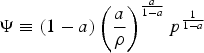 $\Psi\equiv\lpar 1-a\rpar \left({a\over\rho}\right)^{{a\over1-a}}p^{{1\over1-a}}$
and
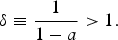 $\delta\equiv{1\over1-a}>1.$
The value of K that maximizes the firm's profit is
 $\left({ap\theta\over\rho}\right)^{\delta}$
. π is a measure of firm size and thus the larger is θ, the larger the firm size.
We model natural hazard by decreasing θ
t
, i.e., a natural calamity can cause damages which reduce the general productivity of the technology in place. Upon the occurrence of such an event the general productivity of the technology instantaneously drops from θ to Yθ, where 0 ≤ Y ≤ 1 is the fraction of productivity in place after a natural disaster has occurred. If Y = 0, then the calamity destroys all the productivity, while if Y = 1, then it has no effect on the productivity. More generally, we assume that the magnitude of the disaster is uncertain. Specifically, we assume that Y is drawn from a power distribution over the interval
 $\lsqb 0\comma \; 1\rsqb $
with parameter
 $\alpha\lpar >0\rpar $
; that is, the distribution function is defined as
 $$F\lpar Y\rpar =Y^{\alpha}\comma \; \rm {with} \, 0\leq Y\leq1$$
and the expected fraction of productivity lost is
 $\open{E}\lpar 1-Y\rpar =\vint_{0}^{1}\lpar 1-Y\rpar \break dF\lpar Y\rpar ={1\over\alpha+1}$
. Hence, an increase in α decreases the expected loss or, otherwise, a larger value of α increases
 $\open{E}\lpar Y\rpar $
, the expected fraction of productivity still in place after the calamity. Equation (1) implies that
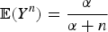 $\open{E}\lpar Y^{n}\rpar ={\alpha\over\alpha+n}$
, provided that α + n > 0.
Also the arrival rate of natural disasters is uncertain. More formally, we assume that the productivity evolves according to a geometric jump-diffusion process
 $$d\theta_{t}=\mu\theta_{t}dt+\sigma\theta_{t}dW_{t}+\lpar Y-1\rpar \theta_{t}dQ_{t}.$$
 $\mu\lpar >0\rpar $
is the instantaneous drift,
 $\sigma\lpar >0\rpar $
is the volatility of the Brownian part of the process, dW
t
is a standard Gauss–Wiener process, and dQ
t
is a Poisson process where
 $dQ_{t}=1 \hbox{with probability } \lambda dt$
and
 $dQ_{t} = 0\ \hbox{with probability} \lpar 1-\lambda dt\rpar $
. The productivity parameter θ as given by (2) has two sources of uncertainty. The term σ dW
t
corresponds to business-as-usual uncertainty, while the term dQ
t
is the jump uncertainty which counts the number of natural hazards. Within an infinitesimally small time interval dt, a jump occurs with probability λ dt; that is, λ denotes the arrival rate of a natural disaster. Throughout the processes W, Q and Y are supposed to be independent.
We define the following function
 $Dis\lpar x\rpar \equiv r-\mu\delta-{1\over2}\sigma^{2}\delta\lpar \delta-1\rpar +{\lambda\delta\over x+ \delta \prime}$
where r is the market interest rate. Note that
 $Dis \lpar x\rpar $
is decreasing in x and let us define
 $Dis \lpar \infty\rpar \equiv lim_{x\rightarrow\infty}{Dis}\lpar x\rpar $
. Throughout the paper we use the following assumption.
Assumption 1
Parameters are such that
 ${Dis}\lpar x\rpar \in\lpar 0\comma \; 1\rpar $
for each x ≥ 0 and that
 $r\in\lpar 0\comma \; 1\rpar $
.
Assumption
 ${Dis}\lpar x\rpar >0$
guarantees that firm values below are well defined, while the assumption
 ${Dis}\lpar x\rpar <1$
requires that λ is sufficiently small; that is, natural disasters are sufficiently rare.
In order to simplify notation we omit the time subscript wherever this does not lead to confusion.
We assume that the firm can reduce the damage caused by a natural disaster through a mitigation investment. In particular, we assume that if the firm spends I, then the probability distribution of the fraction of productivity that is in place after a natural calamity is
 $$F_{I}\lpar Y\semicolon \; I\rpar =Y^{\alpha\lpar I\rpar }\comma \; \rm{with}\, 0\leq Y\leq1\comma \; $$
where
 $\alpha\lpar I\rpar $
is a linear function of I, i.e.,
 $\alpha\lpar I\rpar =\alpha+\varepsilon I\comma \; $
for
 $\varepsilon>0$
. Hence, if the firm does not invest then
 $\alpha\lpar 0\rpar =\alpha$
and thus (3) and (1) are the same. Given two investment levels I′ and I″, where I′ < I″, we have that
 $F_{I}\lpar Y\semicolon \; I''\rpar <F_{I}\lpar Y\semicolon \; I'\rpar $
and thus
 $F_{I}\lpar Y\semicolon \; I''\rpar $
first order stochastically dominates
 $F_{I}\lpar Y\semicolon \; I'\rpar $
. As a consequence, the greater is I, the lower the average damage of a natural calamity, i.e.,
 $\vint_{0}^{1}\lpar 1-Y\rpar dF_{I}\lpar Y\semicolon \; I''\rpar <\vint_{0}^{1}\lpar 1-Y\rpar dF\lpar Y\semicolon \; I'\rpar $
. ε measures how strongly α is increased for a given investment level and thus captures the efficiency of the mitigation investment. The entrepreneur chooses I with the aim of maximizing the mitigation option value and hence the firm value.
The firm's problem is to choose the optimal investment strategy such that the expected present value of its cash flow is maximized. Formally, the following optimal investment problem has to be solved
 $$V\lpar \theta_{0}\rpar =\sup_{I\comma \tau\in\cal{T}}\open{E}_{0}\left\{\vint\limits_{0}^{\infty}\pi\lpar \theta_{t}\rpar e^{-rt}dt-Ie^{-r\tau}\right\}\comma \; $$
subject to equation (2), where Y is distributed according to
 $F\lpar Y\rpar $
for 0 < t ≤ τ, and according to
 $F_{I}\lpar Y\semicolon \; I\rpar $
for t > τ. Assumption 1 guarantees that the integral in (4) is well defined.
 $\cal{T}$
is the class of admissible implementation times conditional on the filtration generated by the stochastic process θ
t
.
The firm value satisfies the following Hamilton–Jacobi–Bellman (H-J-B) equationFootnote 8
 $$rV\lpar \theta\rpar dt=\Psi\theta^{\delta}dt+\open{E}\lpar dV\rpar .$$
Equation (5) has a straightforward economic interpretation. The rate of return consists of the cash flow
 $\Psi\theta^{\delta}$
plus the expected capital gain
 $\open{E}\lpar dV\rpar $
. Optimality requires that the total expected return of the investment equals the market return r. To calculate the expected change in the firm value,
 $\open{E}d\lpar V\rpar $
, we apply Ito's Lemma for jump-diffusion processes to obtain
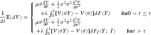 $${1\over dt}\open{E}\lpar dV\rpar = \left\{\matrix{ \mu \theta {\partial V\over\partial\theta} + {1\over2}\sigma^{2}\theta^{2}{\partial^{2}V \over \partial \theta^{2}} \hfill &{} \cr +\lambda\vint_{0}^{1} \lsqb V\lpar \theta Y\rpar - V\lpar \theta \rpar \rsqb dF \lpar Y\rpar &\hbox{for} 0 \lt t \leq \tau \cr \mu \theta {\partial V \over \partial \theta} + {1 \over 2}\sigma^{2}\theta^{2}{\partial^{2}V \over \partial \theta^{2}} \hfill &{} \cr \, + \lambda \vint_{0}^{1}\lsqb V\lpar \theta Y\rpar - V\lpar \theta \rpar \rsqb dF_{I}\lpar Y\semicolon \; I\rpar &\hbox{for}t \gt \tau}\right.$$
We can rewrite the H-J-B equation as follows
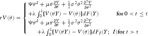 $$rV\lpar \theta\rpar = \left\{\matrix{\Psi\theta^{\delta}+\mu\theta{\partial V\over\partial\theta}+{1\over2}\sigma^{2}\theta^{2}{\partial^{2}V\over\partial\theta^{2}}\hfill &{} \cr +\lambda\vint_{0}^{1}\lsqb V\lpar \theta Y\rpar -V\lpar \theta\rpar \rsqb dF\lpar Y\rpar \quad \quad \quad \hbox{for }0<t\leq\tau\cr \Psi\theta^{\delta}+\mu\theta{\partial V\over\partial\theta}+{1\over2}\sigma^{2}\theta^{2}{\partial^{2}V\over\partial\theta^{2}}\hfill &{} \cr +\lambda\vint_{0}^{1}\lsqb V\lpar \theta Y\rpar -V\lpar \theta\rpar \rsqb dF_{I}\lpar Y\semicolon \; I\rpar \hbox{for }t \gt\tau}\right.$$
We call V d, be and V m, be the value functions in the continuation region (0 < t ≤ τ), where investment is delayed, and termination region (t > τ), where the investment in mitigation has already been undertaken, respectively; the index be indicates that this is the benchmark case, while d and m indicates ‘delay’ and ‘mitigate’, respectively.
Since investment in mitigation is costly, it is undertaken only by firms whose productivity is sufficiently large. In other words, firms have to be sufficiently large for the investment in mitigation to be profitable. The intuition for this result is that if productivity is too low then the costs of a mitigation investment are large compared with its gains and the firm prefers to take its chances and to wait and to weather out the storm. Consequently, the solution to the optimal stopping problem (4) consists of finding a critical productivity level θ
be
, and a corresponding critical firm size
 $\pi\lpar \theta_{be}\rpar $
, above which it is optimal to invest in mitigation. Hence, investment in mitigation should be undertaken the first time the process θ
t
crosses the threshold θ
be
from below.
Consider first the firm value in the termination region V
m, be
. We consider the simple case where only a single investment is allowed, which means that in the termination region there is no further investment option. The general solution to (6) is of the form
 $\Psi_{m}\theta^{\delta}$
, where Ψ
m
is a constant to be determined. Substituting this expression into (6) and solving for V
m, be
we find thatFootnote
9
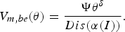 $$V_{m\comma be}\lpar \theta\rpar ={\Psi\theta^{\delta}\over{Dis}\lpar \alpha\lpar I\rpar \rpar }.$$
Assumption 1 assures that (7) is well defined. Equation (7) has a straightforward economic interpretation.
 $V_{m\comma be}\lpar \theta\rpar $
is the expected present value of the profit flow if the productivity level is θ and where the denominator is the discount factor that takes the mitigated expected losses due to natural disasters into account.
When the firm decides to invest in mitigation, the expected payoff is the expected present value of the future profit stream minus the investment cost; that is, the termination payoff is
 $\Omega_{m\comma be}\lpar \theta\semicolon \; I\rpar ={\Psi\theta^{\delta}\over{Dis}\lpar \alpha\lpar I\rpar \rpar }-I.$
The entrepreneur chooses the investment level I that maximizes the value of termination, where
 $$\Omega_{m\comma be}\lpar \theta\rpar =\max_{I}\left[{\Psi\theta^{\delta}\over{Dis}\lpar \alpha\lpar I\rpar \rpar }-I\right]\comma \; $$
and where
 $I_{be}=\hbox{arg}\max_{I}\left[{\Psi\theta^{\delta}\over{Dis}\lpar \alpha\lpar I\rpar \rpar }-I\right]$
.
Consider next the firm value in the continuation region V d, be . It can be verified by direct substitution that a general solution to the differential equation (6) is
 $$V_{d\comma be}\lpar \theta\rpar =\Psi_{d}\theta^{\delta}+\Phi_{1\comma be}\theta^{\phi_{1}}+\Phi_{2\comma be}\theta^{\phi_{2}}+\Phi_{3\comma be}\theta^{\phi_{3}}\comma \; $$
where Φ1, be , Φ2, be and Φ3, be are constants, ϕ1, ϕ2 and ϕ3 are the roots of the characteristic equation
 $${1\over2}\sigma^{2}\phi\lpar \phi-1\rpar +\mu\phi-{\lambda\phi\over\alpha+\phi}=r$$
and
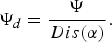 $\Psi_{d}={\Psi\over{Dis}\lpar \alpha \rpar }.$
Assumption 1 assures that Ψ
d
> 0. The last three terms in (9) can be interpreted as the investment option value, while the first term is the expected present value of the profit flow
 $\Psi\theta_{t}^{\delta}$
. Since
 $\alpha\lpar I\rpar >\alpha\comma \; \hbox{Dis}\lpar \alpha\lpar I\rpar \rpar <{Dis}\lpar \alpha\rpar $
and thus
 $\theta^{\delta}\Psi_{d}$
is lower than
 ${\Psi\theta^{\delta}\over{Dis}\lpar \alpha\lpar I\rpar \rpar }$
. The following lemma characterizes the roots of the cubic equation (10).
Lemma 1
The three roots of the characteristic equation (10) are
 $\phi_{2}<-\alpha<\phi_{1}<0<\delta<\phi_{3}$
.
The solution for V d, be must satisfy the following set of boundary conditions
 $$V\lpar 0\rpar =0\comma \; $$
 $$V\lpar \theta\rpar =\Omega\lpar \theta\rpar \comma \; $$
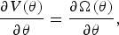 $${\partial V\lpar \theta\rpar \over\partial\theta}={\partial\Omega\lpar \theta\rpar \over\partial\theta}\comma \; $$
computed at
 $\theta=\theta_{be}$
and where V = V
d, be
and
 $\Omega=\Omega_{m\comma be}$
; conditions (11) (12) and (13) determine the constants Φ1, be
, Φ2, be
, Φ3, be
and θ
be
. Condition (11) states that the firm value is zero if productivity is zero which, since the sign of ϕ1 and ϕ2 is negative (see Lemma 1) condition (11), implies that
 $\Phi_{1\comma be}=\Phi_{2\comma be}=0$
. conditions (12) and (13) represent the value matching and smooth pasting condition, respectively, and guarantee that at the investment threshold θ
be
the firm value as well as its derivative are continuous and jointly determine the value of θ
be
and Φ3, be
, ruling out arbitrage possibilities. θ
be
is a free boundary which separates the investment from the no-investment regions. It is also the solution to the stopping problem (4)
 $\tau=\inf\lcub t>0\comma \; \theta\geq\theta_{be}\rcub .$
Proposition 1
The investment threshold is
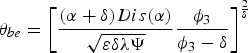 $$\theta_{be}=\left[{\lpar \alpha+\delta\rpar {Dis}\lpar \alpha\rpar \over\sqrt{\varepsilon\delta\lambda\Psi}}{\phi_{3}\over\phi_{3}-\delta}\right]^{{2\over\delta}}$$
and the size of the investment is
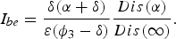 $$I_{be}={\delta\lpar \alpha+\delta\rpar \over\varepsilon\lpar \phi_{3}-\delta\rpar }{{Dis}\lpar \alpha\rpar \over{Dis}\lpar \infty\rpar }.$$
Corollary 1
The value function
 $V_{d\comma be}\lpar \theta\rpar $
and the value of termination
 $\Omega_{m\comma be}\lpar \theta\rpar $
are increasing in ε.
For a given investment level, the larger is ε, the more efficient are mitigation investments and the lower the average damage of a catastrophic event. From Proposition 1 we can observe that θ be and I be are decreasing in ε. Thus, taking into account the results stated in Corollary 1, we can conclude that, the larger is ε, the lower the optimal investment in mitigation, the lower the critical level of the firm's productivity that triggers investment, that is, the earlier the investment is undertaken, and the larger the firm value.
4. The mitigation investment decision with financial aid
In this section we study how financial aid, if perfectly anticipated by firms, affects their mitigation investment strategy. Financial assistance through donations is provided to help individuals in the recovery process and to alleviate the financial burden they may experience after a natural disaster. In particular we study how charity affects the investment threshold and the size of the investment. We first consider cash aid in the form of an instantaneous cash flow and afterward we consider an in-kind aid program aimed at restoring firm's productivity. We assume that the instantaneous cash flow cannot be used to restore the firm's productivity. The analysis below could be extended to the case where the cash flow is partially used to restore productivity without altering our qualitative results. We indicate with index ca investment trigger and value functions if financial aid is in the form of cash, while with re if aid is targeted in the form of a productivity restoration program.
4.1. Cash aid
Throughout this section we assume that upon occurrence of a natural calamity the firm receives an instantaneous cash flow. More formally, we assume that a natural disaster triggers a cash flow proportional to firm profits prior to the eventFootnote 10
 $$Aid_{t}dt=\kappa\lpar 1-Y^{\delta}\rpar \Psi\theta_{t}^{\delta}dQ_{t}\comma \;$$
where
 $0<\kappa\leq1$
is an exogenous donation rate. The expected instantaneous cash flow due to donations without mitigation investment, where Y is distributed according to
 $F\lpar Y\rpar $
in (1), is
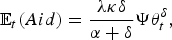 $$\open{E}_{t}\lpar Aid\rpar ={\lambda\kappa\delta\over\alpha+\delta}\Psi\theta_{t}^{\delta}\comma \;$$
which is increasing in the donations rate κ, the arrival rate of natural disasters λ and also in the severity of the disaster as measured by the damages caused (the lower α, the more severe the damages). The reason for this latter assumption is that the more adverse the effects of a calamity, the greater the worldwide news coverage, and therefore the more funds will be raised.Footnote 11
With financial charity the firm's investment problem is
 $$V\lpar \theta_{0}\rpar =\sup_{I\comma \tau_{ca}\in\cal{T}}\open{E}_{0}\left\{\vint\limits_{0}^{\infty}e^{-rt}\Psi\theta_{t}^{\delta}dt+\vint\limits_{0}^{\infty}e^{-rt}\kappa\lpar 1-Y^{\delta}\rpar \Psi\theta_{t}^{\delta}dQ_{t}-Ie^{-r\tau_{ca}}\right\}\comma \;$$
subject to equation (2), where for
 $0<t\leq\tau_{ca}$
the distribution of Y is
 $F\lpar Y\rpar $
, while for t > τ
ca
it is
 $F_{I}\lpar Y\semicolon \; I\rpar $
.
Following the argument in the previous section we must calculate the expected discounted present value of the termination value with cash aid
 $$\open{E}_{0}\left[\vint\limits_{0}^{\infty}e^{-rt}\Psi\theta_{t}^{\delta}dt+\vint\limits_{0}^{\infty}e^{-rt}\kappa\lpar 1-Y^{\delta}\rpar \Psi\theta_{t}^{\delta}dQ_{t}\right]\comma \;$$
where the dynamics of θ
t
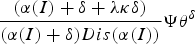
are given by (2) with Y distributed as explained above. Following the calculations presented in the online appendix we can show that the expected present value of the termination cash flow is
 ${\lpar \alpha\lpar I\rpar +\delta+\lambda\kappa\delta\rpar \over\lpar \alpha\lpar I\rpar +\delta\rpar {Dis}\lpar \alpha\lpar I\rpar \rpar }\Psi\theta^{\delta}$
. Hence, the termination payoff is
 $\Omega_{m\comma ca}\lpar \theta\semicolon \; I\rpar ={\lpar \alpha\lpar I\rpar +\delta+\lambda\kappa\delta\rpar \over\lpar \alpha\lpar I\rpar +\delta\rpar {Dis}\lpar \alpha\lpar I\rpar \rpar }\Psi\theta^{\delta}-I$
and the entrepreneur chooses the investment level I that maximizes the value of termination, where
 $$\Omega_{m\comma ca}\lpar \theta\rpar =\max_{I}\left\{{\lpar \alpha\lpar I\rpar +\delta+\lambda\kappa\delta\rpar \over\lpar \alpha\lpar I\rpar +\delta\rpar {Dis}\lpar \alpha\lpar I\rpar \rpar }\Psi\theta^{\delta}-I\right\}$$
and where
 $I_{ca}=\hbox{arg}\max_{I}\left\{{\lpar \alpha\lpar I\rpar +\delta+\lambda\kappa\delta\rpar \over\lpar \alpha\lpar I\rpar +\delta\rpar {Dis}\lpar \alpha\lpar I\rpar \rpar }\Psi\theta^{\delta}-I\right\}$
.
In the continuation region d the firm does not invest in mitigation and the firm value is implicitly defined by the fundamental equation of optimality
 $$rV_{d\comma ca}\lpar \theta\rpar dt=\Psi\theta^{\delta}dt+\kappa\open{E}\lsqb \lpar 1-Y^{\delta}\rpar dQ_{t}\rsqb \Psi\theta_{t}^{\delta}+\open{E}\lpar dV_{d\comma ca}\rpar \comma \;$$
where the second term on the right-hand side is the expected cash flow due to financial aid. We apply Ito's Lemma for jump-diffusion processes to obtain
 $$\eqalign{rV_{d\comma ca}\lpar \theta\rpar &=\Psi\theta^{\delta}+\kappa\lambda\Psi\theta^{\delta}\vint_{0}^{1}\lpar 1-Y^{\delta}\rpar dF\lpar Y\rpar +\mu\theta{\partial V_{d\comma ca}\over\partial\theta}+{1\over 2}\sigma^{2}\theta^{2}{\partial^{2}V_{d\comma ca}\over\partial\theta^{2}}\cr &\quad+ \lambda\vint_{0}^{1}\lsqb V_{d\comma ca}\lpar \theta Y\rpar -V_{d\comma ca}\lpar \theta\rpar \rsqb dF\lpar Y\rpar \comma \; }$$
It can be easily verified by direct substitution that a general solution to this differential equation is
 $V_{d\comma ca}\lpar \theta\rpar ={\lpar \alpha+\delta+\kappa\lambda\delta\rpar \Psi\theta^{\delta}\over\lpar \alpha+\delta\rpar {Dis}\lpar \alpha\rpar }+\Phi_{3\comma ca}\theta^{\phi_{3}}\comma \; $
where Φ3, ca
is a constant to be determined and ϕ3 is the positive root of the characteristic equation (10).
The solution for V
d, ca
must satisfy the absorbing barrier (11), value matching (12) and smooth pasting (13) conditions at the critical threshold θ
ca
, with
 $\Omega=\Omega_{m\comma ca}$
.
Proposition 2
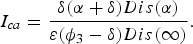
The investment threshold is
 $$\theta_{ca}=\left[{\lpar \alpha+\delta\rpar {Dis}\lpar \alpha\rpar \over\sqrt{\varepsilon\delta\lambda\Psi\lsqb 1-\kappa {Dis}\lpar \infty\rpar \rsqb }}{\phi_{3}\over\phi_{3}-\delta}\right]^{{2\over\delta}}>0\comma \;$$
and the size of the investment is
 $$I_{ca}={\delta\lpar \alpha+\delta\rpar {Dis}\lpar \alpha\rpar \over\varepsilon\lpar \phi_{3}-\delta\rpar {Dis}\lpar \infty\rpar }.$$
In the following proposition we compare investment thresholds θ ca and θ be and investment sizes I ca and I be .
Proposition 3
The optimal investment threshold with cash aid, θ ca , is increasing in the donation rate κ and it is always larger than the optimal investment threshold without financial aid, θ be . The size of the investment with and without cash aid is the same.
Financial charity has the effect of increasing the critical productivity size above which investment in mitigation is optimal, thereby delaying the investment. The greater the donation rate κ, the larger the critical productivity size and thus the later the firm invests in mitigation. Note that even for κ = 1, that is, the case where the cash flow from the international donor is equal to the size of the damage, investing in mitigation is still optimal for sufficiently productive firms. The reason for this result is that the donor's cash flow is not (or cannot) be used for restoring the firm's productivity. Since what matters for the firm value is the productivity level, investing in mitigation in order to reduce the damage caused by natural hazards is still optimal if the firm is sufficiently productive.
Cash aid produces two effects on the investment size. First, for a given productivity level θ, it has a direct negative effect because the expectation of financial assistance crowds out private investments. Secondly, since it increases the critical productivity threshold, it has an indirect positive effect on the investment size. The two exactly offset each other and thus the overall effect of cash aid on the investment size is nil.
4.2. In-kind aid
In this section we consider in-kind aid programs that aim at restoring productivity (i.e., plants, factories, machinery) destroyed by natural disasters. Let the probability distribution of the fraction of productivity in place after the occurrence of a natural disaster with in-kind aid, be
 $$F_{\xi}\lpar Y\semicolon \; \xi\rpar =Y^{\alpha\lpar \xi\rpar }\comma \; \hbox{with }0\leq Y\leq1\comma \; $$
where ξ captures the size of financial relief and
 $\alpha\lpar \xi\rpar $
is a linear function of ξ, i.e.,
 $\alpha\lpar \xi\rpar =\alpha+\xi$
. Consider ξ′ and ξ″, where ξ′ > ξ″, then
 $F_{\xi}\lpar Y\semicolon \; \xi'\rpar $
first order stochastically dominates
 $F_{\xi}\lpar Y\semicolon \; \xi''\rpar $
. As a consequence the larger is ξ, the lower the expected productivity loss. For ξ = 0 financial aid is zero and thus (1) and (15) are the same, while for
 $\xi\rightarrow\infty$
productivity restoration is complete.
Akin to the previous sections, we assume that if the firm invests I in mitigation, then the probability distribution of the fraction of productivity that survives a catastrophic event is
 $$F_{\xi I}\lpar Y\semicolon \; I\comma \; \xi\rpar =Y^{\alpha\lpar I\comma \xi\rpar }\comma \; \hbox{with }0\leq Y\leq1\comma \;$$
where
 $\alpha\lpar I\comma \; \xi\rpar =\alpha+\varepsilon I+\xi$
.
The firm's problem is to choose the optimal investment strategy such that the expected present value of its cash flow is maximized. Formally, the optimal investment problem (4) has to be solved, subject to equation (2), where Y is distributed according to
 $F_{\xi}\lpar Y\semicolon \; \xi\rpar $
for
 $0<t\leq\tau_{re}$
, and according to
 $F_{\xi I}\lpar Y\semicolon \; I\comma \; \xi\rpar $
for t > τ
re
and where the subscript re indicates that a restoration program is in place.
If the firm decides to invest in mitigation, then the expected payoff is the expected present value of the future profit stream minus the investment cost. Thus, the value of termination can be written as
 $$\Omega_{m\comma re}\lpar \theta\semicolon \; I\rpar ={\Psi\theta^{\delta}\over{Dis}\lpar \alpha\lpar I\comma \; \xi\rpar \rpar }-I\comma \; $$
The entrepreneur chooses the investment level I that maximizes the value of termination
 $$\Omega_{m\comma re}\lpar \theta\rpar =\max_{I}\left\{{\Psi\theta^{\delta}\over{Dis}\lpar \alpha\lpar I\comma \; \xi\rpar \rpar }-I\right\}\comma \;$$
where
 $I_{re}=\hbox{arg}\max_{I}\left\{{\Psi\theta^{\delta}\over{Dis}\lpar \alpha\lpar I\comma \; \xi\rpar \rpar }-I\right\}$
.
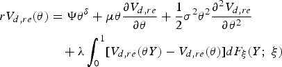
In the continuation region d, where investment in mitigation is delayed, the firm value is implicitly defined by the fundamental equation of optimality
 $$\eqalign{rV_{d\comma re}\lpar \theta\rpar &=\Psi\theta^{\delta}+\mu\theta{\partial V_{d\comma re}\over\partial\theta}+{1\over2}\sigma^{2}\theta^{2}{\partial^{2}V_{d\comma re}\over\partial\theta^{2}}\cr &\quad+\lambda\vint_{0}^{1}\lsqb V_{d\comma re}\lpar \theta Y\rpar -V_{d\comma re}\lpar \theta\rpar \rsqb dF_{\xi}\lpar Y\semicolon \; \xi\rpar }$$
It can be easily verified by direct substitution that a general solution to this differential equation is
 $V_{d\comma re}\lpar \theta\rpar ={\Psi\theta^{\delta}\over{Dis}\lpar \alpha\lpar \xi\rpar \rpar }+\Phi_{3\comma re}\theta^{\phi_{3}}\comma \; $
where Φ3, re
is a constant to be determined and ϕ3 is the positive root of the characteristic equation (10). Assumption 1 assures that
 ${Dis}\lpar \alpha\lpar \xi\rpar \rpar >0$
.
The solution for V
d, re
must therefore satisfy the absorbing barrier (11), value matching (12) and smooth pasting (13) conditions at the critical threshold θ
re
, with
 $\Omega=\Omega_{m\comma re}$
.
Proposition 4
The investment threshold is
 $$\theta_{re}=\left[{\lpar \alpha+\delta+\xi\rpar {Dis}\lpar \alpha\lpar \xi\rpar \rpar \over\sqrt{\varepsilon\delta\lambda\Psi}}{\phi_{3}\over\phi_{3}-\delta}\right]^{{2\over\delta}}\comma \;$$
and the size of the investment is
 $$I_{re}={\delta\lpar \alpha+\delta+\xi\rpar {Dis}\lpar \alpha\lpar \xi\rpar \rpar \over\varepsilon\lpar \phi_{3}-\delta\rpar {Dis}\lpar \infty\rpar }.$$
From a comparison between the investment thresholds with restoration program θ re and without restoration θ be we can get the following result.
Proposition 5
The optimal investment threshold with restoration program, θ re , is increasing in ξ and it is always larger than the optimal investment threshold without financial aid, θ be . The size of the investment with the restoration program is larger than the one without it.
These results show that in-kind aid delays mitigation investments and that the critical threshold level above which firms invest in mitigation is increasing in the size of financial relief. Note that as ξ becomes infinitely large the productivity threshold, and hence the critical firm size, becomes infinitely large and thus the firm never invests in mitigation. This result is very intuitive: if financial restoration programs cover all losses by restoring productivity to its previous level, then the firm never has an incentive to engage in costly investments that reduce damages to productivity due to natural calamities. Akin to cash aid, in-kind aid produces two effects on the investment size. First, for a given productivity level θ, it affects the investment size negatively because of a crowding-out effect. Secondly, since it increases the critical productivity threshold, it has an indirect positive effect on the investment size. This latter effect is stronger than the former one and thus the overall effect of in-kind aid on the investment size is positive. Note that θ re and I re are both increasing in ξ, and thus the greater is the financial aid, the later the firm invests in mitigation, i.e., the larger the firm size, the larger is the investment size, that is, the lower is the average damage of natural hazards.Footnote 12
4.3. International donor: cash aid versus in-kind aid
In this section we consider the international donor's problem who has to choose between cash aid and in-kind aid. For this purpose we assume that the donor's objective function depends negatively on the time of the investment, that is, the critical productivity size above which firms decide to invest in mitigation, and positively on the investment size. We restrict ourself to the case where all aid is either in cash or in kind, even though the analysis could be straightforwardly extended to the case of mixed strategies where the optimal policy mix could be identified. We assume that the international donor maximizes her objective function under the constraint that the economic value for the recipient is on average the same under both strategies.
Cash aid consists of a cash flow in the case of a natural disaster while in-kind aid entails the (partial) restoration of the firm's productivity to pre-disaster levels. We require the effects of the two policies in terms of firm profits to be on average the same. Since we are interested in comparing investment triggers we require the value of the two aid strategies to be equal before the investment has been undertaken. Formally, we require that
 $$\kappa\vint_{0}^{1}\lsqb \lpar 1-Y^{\delta}\rpar \Psi\theta_{t}^{\delta}\rsqb dF\lpar Y\rpar =\vint_{0}^{1}\Psi\lpar Y\theta_{t}\rpar ^{\delta}dF_{\xi}\lpar Y\semicolon \; \xi\rpar -\vint_{0}^{1}\Psi\lpar Y\theta_{t}\rpar ^{\delta}dF\lpar Y\rpar $$
The left-hand side is the expected cash flow of the cash aid program, while the right-hand side is the expected value in terms of firm profits of the in-kind aid program.
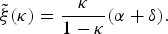
Rearranging this equality we obtain for a given κ the critical value
 $\tilde{\xi}\lpar \kappa\rpar $
such that the economic value of the two programs is on average the same
 $$\tilde{\xi}\lpar \kappa\rpar ={\kappa\over 1-\kappa}\lpar \alpha+\delta\rpar .$$
Proposition 6
For any ξ > 0 and κ > 0, the optimal investment size with in-kind aid, I
re
, is larger than the optimal investment size with cash aid I
ca
and without financial aid, I
be
. For any κ and
 $\xi=\tilde{\xi}\lpar \kappa\rpar $
,
 $\theta_{re}>\theta_{ca}>\theta_{be}$
.
The first part of Proposition 6 follows straightforwardly from Proposition 3 and Proposition 5: the investment size with in-kind aid is larger than the one with cash aid and without aid. Moreover, since I re is increasing in ξ, the greater the economic value of in-kind aid, the greater is the difference between the investment sizes. The second part of Proposition 6 states that the investment threshold with a restoration program is always larger than the investment threshold with cash aid which is always larger than the investment threshold without financial aid. The intuition for this latter result is that cash aid, by assumption, cannot be used to restore the firm's productivity and thus the effect of an increase in the donation rate on the critical investment threshold is small. On the other side, in the case of in-kind aid, productivity is directly restored and thus the firm has a much weaker incentive to engage in mitigation investments.
Many residents living in hazard-prone areas rarely undertake loss prevention measures to protect their property. Proposition 6 gives us a policy indication to cope with this reluctance by firms to invest in mitigation. If the goal of the policy maker is to provide incentives to speed up investments in loss reduction measures or, put differently, if its aim is to reduce the critical productivity size above which mitigation investments are optimal, then cash aid is preferable to in-kind aid. On the contrary, if the policy maker's aim is to increase the size of the investment and thus to reduce the average damage caused by natural disasters then in-kind aid is preferable. If we allow also for mixed policies and if the donor places more importance on the timing, then the optimal donation strategy consists of relatively more cash, while if greater weight is placed on the investment size, then the optimal donation strategy consists of relatively more in-kind aid.
5. Numerical application
In this section we provide a calibration of the model to illustrate the magnitude of effects and model dynamics. We use data on St Lucia taken from the FAO's reports on hurricane hazard mitigation investments in Latin America and the Caribbean and data for natural disasters taken from EM-DAT: the OFDA/CRED Emergency Disasters Database.
St Lucia, is a small developing country located in the tropical hurricane belt, south of Martinique and north of St Vincent in the Caribbean Sea. Due to its small size and relative lack of geological resources, its economy relies primarily on the sale of banana crops and income generated from tourism, with additional inputs from small-scale enterprises (especially livestock and manufacturing) and fishery. Due to its geographic location in the hurricane belt as well as in a tectonically active area, St Lucia is regularly exposed to natural hazards including tropical storms, hurricanes, floods, localized floods, drought spells, landslides and earthquakes, which regularly affect the agriculture, tourism and livestock sectors. Small ruminants are an important livelihood asset of farmers. According to the FAOFootnote 13 there is at present no meaningful or effective catastrophe coverage for vulnerable farmers with very few exceptions for banana/crop producers. Livestock farmers in St Lucia have no means to transfer risks, hence they are extremely vulnerable to natural disasters. To cope with this lack of insurance coverage for small-scale farmers we consider the construction of a hurricane-resistant small ruminant shelter.
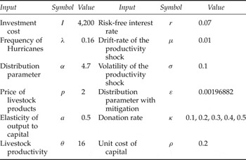
Table 1 summarizes the base-case parameter values. A detailed description of how parameters have been obtained can be found in the online appendix. We carry out simulations with the intent to investigate investment thresholds and investment sizes and how they are affected by financial aid.
Summary of base-case parameter values

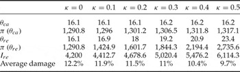
First, as predicted by theory, simulation results show that a restoration program increases the critical productivity size much more than cash aid. Thus, while cash aid has only a weak impact on the critical productivity size, from Table 2 we observe that a restoration program has a much stronger impact on the investment decision. Secondly, we observe that, in the case of a restoration program, the size of the investment is increasing in the donation rate, which also implies that the expected damage after the investment has been undertaken is decreasing in the donation rate. Table 2 evidences the tradeoff the international donor is facing: cash aid leads to a lower critical productivity size but also to a lower investment level (which implies a higher average damage), while a productivity restoration program leads to a larger critical productivity size but also a larger investment level (which implies a lower average damage). Thus, if firms are heterogeneous in their productivity, then increasing the donation rate, by increasing the critical productivity size, induces fewer firms to invest in mitigation. Moreover, if aid is in the form of a restoration program then firms investing will invest more than if aid is in cash, even though fewer firms will invest.
Critical thresholds for r=0.07; donation rates κ=0, 0.1, 0.2, 0.3, 0.4 and 0.5; I=4200 and ε=0.00201499

We carry out some sensitivity analysis by increasing the calibrated cost of the investment I from I
ca
 $=I_{be}= \$ 4{\comma \; }200$
to I
ca
=I
be
= US$ 4,300. Note that this is equivalent to assuming a lower efficiency of the investment ε. In particular, by calibrating the model assuming I
ca
=I
be
= US$ 4,300 we obtain
 $\varepsilon=0.00224002$
, which is lower than the one obtained in the previous case, while the expected damage after investment remains unchanged (12.2 per cent).Footnote
14
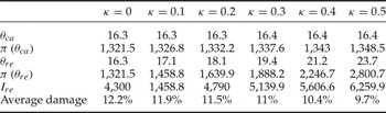
From Table 3 we observe that an increase in I by approximately 2.38 per cent increases the investment thresholds by the same percentage. Hence innovations that increase the effectiveness of mitigation investments lead to earlier adoptions and to lower investment sizes, without affecting the expected damage after the investment.
Critical thresholds for, r=0.07; donation rates κ=0, 0.1, 0.2, 0.3, 0.4 and 0.5; I=4300 and ε=0.00224002

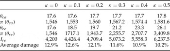
In Table 4 we show simulation results for investment costs I ca =I be = US$ 4,200 if the interest rate raises from 0.07 to 0.075. Compared with the baseline simulation results in Table 2 US$ 4,200 we observe that a small increase in the interest rate strongly increases the investment triggers. Hence policies that reduce the real interest rate have the effect of reducing investment thresholds, thereby speeding up mitigation investments.
Critical thresholds for r=0.075; donation rates κ=0, 0.1, 0.2, 0.3, 0.4 and 0.5; I=4200 and ε=0.00208388

6. Conclusions
Disaster involving natural hazards can have devastating short-and long-term impacts on the society and the economy of any country, adversely affecting progress towards sustainable development. They cause loss of life, social disruption and affect economic activities. The general increase in vulnerability of societies worldwide has motivated the 2005 United Nations World Conference on Disaster Reduction and its resulting report, the Hyogo ‘Framework for Action’, which emphasizes the need for proactive disaster management including cost-effective risk reduction investments and where this is not possible, risk transfer through insurance and other catastrophe-linked securities (i.e., Cat Bonds). In this paper we analyze how international aid programs in the form of cash transfer and in-kind aid affect mitigation investments such as the inclusion of specific safety or vulnerability reduction measures in the design and construction of new facilities, the retrofitting of existing facilities against seismic risk, or the building of structural flood defense measures, and do not consider risk transfer through insurance and other financial markets instruments. We find that: (1) both financial aid strategies increase the critical productivity size thereby delaying investment in mitigation; (2) in-kind aid increases the critical productivity size more than cash aid does and thus delays investment in mitigation more than under a cash aid program; and (3) cash aid does not alter the size of the mitigation investment, while in-kind aid increases it. These results have important implications for international donors. Donors may want to accelerate the adoption of measures reducing the vulnerability of small firms. In this case they should provide relief in the form of cash aid which outperforms in-kind aid and speeds up investment in mitigation. On the contrary, if their aim is to reduce the average damage caused by natural hazards, then in-kind aid is preferable.
Some extensions and further directions of research might be fruitful. One is to incorporate environmental risk, accounting for the uncertainty in the arrival rate of catastrophic events or in the future costs of environmental damage. Another extension would be taking informational asymmetries into account, by assuming that the international donor cannot observe the damage caused by natural hazards, and to solve the corresponding principle-agent problem.