Introduction
High-strength steels have wide-ranging applications in the transportation industry due to their excellent energy absorption, light weight, and low fuel consumption. High-strength low-alloy steels have high yield strength, high ratio of yield stress to ultimate tensile stress, and good resistance to deformation. They are usually used as structural parts and reinforcements such as longitudinal beam, crossbeams of the body in white. Many studies [Reference Oyyaravelu, Kuppan and Arivazhagan1, Reference Han, Xie, Xiong, Shang and Misra2, Reference Macwan, Kumar and Chen3, Reference Li, Wan, Lu, Shirzadi, Isayev, Hress and Wu4] have been conducted on high-strength low-alloy steels that possess high strength, good cold formability, and good weldability.
In recent years, describing the tensile properties of materials at elevated strain rates is gaining increasing attention. Since deformation of materials during the impact is a dynamic response, studying and simulating the mechanical response of materials at elevated strain rates have a guidance role on optimizing the structural design, reasonably selecting the materials, and improving the vehicle body safety. The mechanical behavior of materials at high strain rates is considerably different from that observed at quasi-static loads because of the strain rate sensitivity of materials [Reference Khan, Baig, Choi, Yang and Sun5, Reference Kim, Kim, Han, Barlat and Lee6, Reference Wang, Li, He, Wei, Wang and Du7, Reference Qin, Chen, Wen, Lin, Liang and Lu8, Reference Singh, Cadoni, Singha and Gupta9, Reference Fathi, Emadoddin and Mohammadian Semnani10]. Wang et al. [Reference Wang, Li, He, Wei, Wang and Du7] reported on investigations into the dynamic tensile properties of high-strength 600–1000-MPa dual-phase steel and 1200 MPa fully martensitic (MS) steel under elevated strain rates. The research results indicated that all investigated dual-phase steels had a positive strain rate dependency. However, negative strain rate dependency was observed for 1200 MPa MS. Qin et al. [Reference Qin, Chen, Wen, Lin, Liang and Lu8] studied the mechanical responses of two dual-phase high-strength steels (DP700 and DP500) under dynamic loading. Results showed the significant differences between quasi-static and dynamic tensile behavior in terms of the ultimate tensile stress, yield stress, uniform elongation, and total elongation. However, it is usually assumed that the measurement area of the test specimen is a uniform stress–strain distribution. When deformation of the gauge region exceeds the point of uniform elongation, it will concentrate in the local area, which is known as strain localization. At this time, the information extracted from the stress–strain curves is controversial in its effectiveness. An alternative method is required when extracting the local deformation behavior from the overall response of the gauge region in test specimen.
To acquire more local behavior of the gauge region in the test sample, the digital image correlation (DIC) technique is usually used. Some important local deformation information of materials, such as the fracture strain which is likely hard to gain in other ways, can be acquired through DIC technique. In numerical simulations, the fracture strain often plays an important role in determining an element’s failure. This crucial parameter can be obtained by DIC which is capable of detecting traces of the speckles sprayed on the gauge region surface of experimental samples. In addition, DIC technique has been widely used in the field of deformation field measurement [Reference Smith, Higgins and Sampath11, Reference Valeri, Koohbor, Kidane and Sutton12, Reference Flores, Mollenhauer, Runatunga, Beberniss, Rapking and Pankow13, Reference Tarigopula, Hopperstad, Langseth, Clausen and Hild14, Reference Wu, Mao, Zhou and Lu15, Reference Chen, Niu, Lian and Lin16, Reference Kammers, Wongsangam, Langdon and Daly17]. Valeri et al. [Reference Valeri, Koohbor, Kidane and Sutton12] used DIC technique to predict the uniaxial stress–strain response of the 304 stainless steel at high temperature. Wu et al. [Reference Wu, Mao, Zhou and Lu15] used the DIC technique to monitor the full-field strain of the system including brittle coating and ductile substrate during tension tests. Accordingly, DIC technique has been implemented in many study fields, such as crack propagation, full-field deformation, and damage threshold strain. However, DIC technique is not frequently implemented to obtain the stress–strain curve of materials at elevated strain rates. One of the purposes of this paper is to evaluate the performance of DIC strain measurement in high-speed tensile experiments.
Finite element simulation is a reliable approach to obtain the full-field deformation information of test samples. By this means, stress and strain distribution and local deformation behavior of experimental specimens can be easily evaluated. Selection of material models will greatly determine the availability of numerical simulation. At present, a large number of constitutive models have been used to depict the true mechanical response of metallic materials, such as the Johnson–Cook (J–C) model [Reference Peirs, Verleysen, Paepegem and Degrieck18, Reference Zhao, Sun, Li, Yan and Wang19, Reference Chang, Zhou, Peng, Li and He20, Reference Sahu, Mondal, Goel, Ansari and Ansari21], Cowper–Symonds model [Reference Chen, Li and Li22], and Zerilli–Armstrong model [Reference Gurusamy and Rao23]. To represent the strain rate sensitivity observed in the experiments for the investigated steel, the J–C model was selected due to its simplicity, good prediction, and the validity of parameters [Reference Peirs, Verleysen, Paepegem and Degrieck18].
In this paper, the strain rate sensitivity on the mechanical behavior of high-strength low-alloy (HC420LA) steel was investigated. The uniaxial tensile tests over various strain rates ranging from 0.001 to 500 s−1 were performed. The full-field strain distribution in tensile samples was acquired by means of DIC technique. The stress–strain curves of the point near the fracture crack were presented at six strain rates. Based on experimental results, the influences of strain rate on the tensile properties were assessed. A modified J–C model was used to describe strain rate sensitivity of mechanical performance, and numerical simulation of the representative test at a strain rate of 100 s−1 was modeled. Finally, the strain field and axial strain–time curves were used for validating the numerical simulations.
Results and discussion
Stress–strain relationship
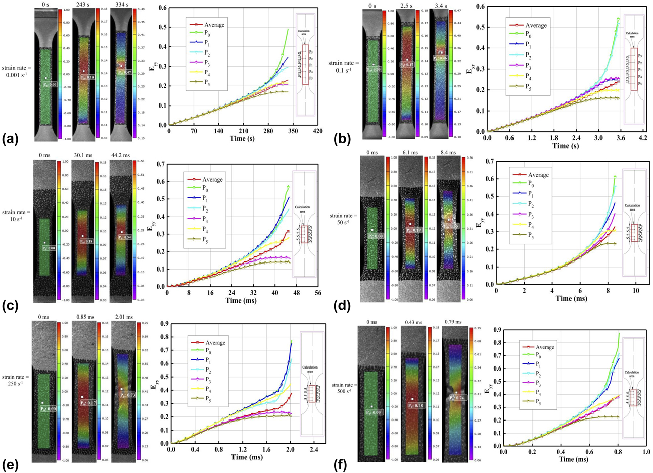
Tensile experiments were performed under uniaxial impact loading; therefore, only the axial strain (E yy) was calculated and analyzed. The parallel length of the specimen was selected as the calculation area. Meanwhile, the calculation area was divided into a number of calculation subsets, and the calculation subset size was 29 × 29 pixels. Although DIC was known as a local measurement technique, the single-point strain cannot be acquired directly. In fact, the strain was calculated from the average strain of several adjacent calculation subsets, so the strain at the edge could not be determined. The strain cloud map of the calculation area was obtained using DIC technique. Meanwhile, strain–time curves of some special points distributed on the specimen surface sprayed with speckle and the average strain curve of the calculation area were extracted. P 0 was the point near the fracture crack. P 1, P 2, P 3, P 4, and P 5 were five reference points distributed on the tensile axis of the specimen, among which P 1 was the center of the specimen. The distance between two adjacent reference points at the high strain rate and the low strain rate was 5 mm and 12.5 mm, respectively. The cloud maps of E yy and the strain–time curves are shown in Fig. 1. Meanwhile, DIC analysis results of the tensile process are listed in Supplementary material Table SI. For six strain rates, the time corresponding to the maximum load was 243 s, 2.5 s, 30.1 ms, 6.1 ms, 0.85 ms, and 0.43 ms, respectively. When the time exceeded the maximum load time, deformation concentrated near the fracture crack and the strain of the points far from the fracture crack changed very little. E yy of P 0 was larger than the average E yy of the parallel length at the same strain rate. In addition, as the tensile process progressed, the deviation between them became more and more obvious due to the strain localization. For six strain rates, the fracture time of the specimens was 336 s, 3.5 s, 45.6 ms, 8.5 ms, 2.02 ms, and 0.81 ms, respectively. This showed that the fracture time decreased with the increase in tensile velocity. According to DIC analysis results, with the increase in strain rate, the ultimate average E yy increased from 0.230 to 0.392 and the fracture strain (P 0) increased from 0.492 to 0.876.
E yy cloud map and strain–time curves of the calculation area: (a) strain rate = 0.001 s−1, (b) strain rate = 0.1 s−1, (c) strain rate = 10 s−1, (d) strain rate = 50 s−1, (e) strain rate = 250 s−1, and (f) strain rate = 500 s−1.

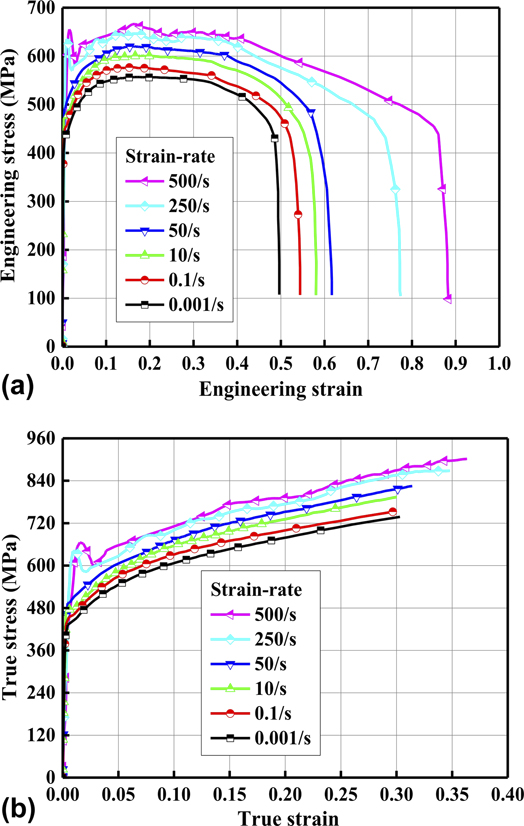
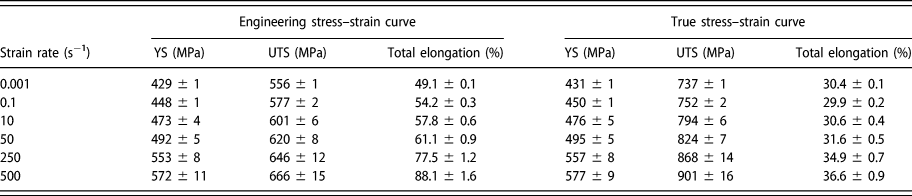
Both quasi-static and dynamic experimental data were used to plot stress–strain curves at various strain rates ranging from 0.001 to 500 s−1. Engineering strain data were obtained from E yy of P 0. Load data were obtained from the force sensor of the high-speed testing machine. Engineering stress–engineering strain curves at six strain rates of HC420LA steel are shown in Fig. 2(a). Meanwhile, true stress–true strain curves are presented in Fig. 2(b). The key experimental data of HC420LA are summarized in Table I (YS is the yield stress at 0.2% offset strain, and UTS is the ultimate tensile stress). Mean and standard deviation listed were the statistical results of three repetitive experiments for each situation. For quasi-static tensile experiments, engineering YS was 429 MPa and engineering UTS was 556 MPa; meanwhile, the corresponding true YS and true UTS were 431 MPa and 737 MPa, respectively. It could be inferred that HC420LA steel exhibited significant strain hardening. Consistent situations could be seen at elevated strain rates. Furthermore, the slopes of six curves between true YS and true UTS were almost parallel, as shown in Fig. 2(b). Therefore, there was little change in terms of strain hardening with strain rates increasing.
Comparison of stress–strain curves of HC420LA steel at strain rates ranging from 0.001 to 500 s−1: (a) engineering stress–engineering strain curves and (b) true stress–true strain curves.

Experimental results of HC420LA steel.

Obvious differences could be observed between quasi-static and dynamic experimental results. It could be concluded that HC420LA steel had a positive strain rate dependence in terms of the ultimate tensile stress, yield stress, and total elongation. Plastic flow stress levels increased as strain rates increased from 0.001 to 500 s−1. The increase in the strength along with the increasing strain rate was well known for strain-rate-sensitive materials [Reference Kim, Kim, Han, Barlat and Lee6]. In addition, the value of engineering total elongation increased from 49.1 to 88.1%. Accordingly, ductility of HC420LA steel was higher under impact loads compared to that under quasi-static loads. That total elongation increased as strain rates increased implied the remarkable influence of strain rate on formability of HC420LA steel. The strain rate of the strain localization area was greater compared to that of the nonlocalized area, so the strength of the strain localization area increased on account of the positive strain rate sensitivity. This resulted in the improvement in strength in the strain localization region and the delay in the propagation of localization. Since the area under stress–strain curves was higher under dynamic strain rates, the fracture energy of the investigated steel was greater under dynamic loads compared to that under quasi-static loads. In addition, at six strain rates (0.001, 0.1, 10, 50, 250, and 500 s−1), the engineering uniform elongation corresponding to the engineering UTS was 17.8%, 17.3%, 17.7%, 17.3%, 17.4%, and 17.6%, respectively. Therefore, the engineering uniform elongation was nearly insensitive to strain rate.
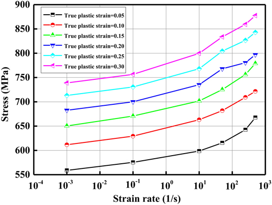
To study the effect of strain rate and strain on the material’s true stress, true stress at different strain rates with reference plastic strains of 0.05, 0.10, 0.15, 0.20, 0.25, and 0.30 was analyzed as shown in Fig. 3. The six reference strains were selected according to true stress–true strain curves of the material, as shown in Fig. 2(b). As the minimum reference plastic strain, 0.05 was chosen to avoid the largest stress oscillation in the initial yielding phase. The other five reference plastic strains were selected to make them uniformly distributed throughout the tensile fracture process of the specimen. True stress increased obviously with the increase in strain rate, which showed the strong strain rate enhancement effect. Under six reference plastic strains (0.05, 0.10, 0.15, 0.20, 0.25, and 0.30), true stress increased by 19.5%, 18.0%, 19.8%, 16.8%, 18.2%, and 18.8%, respectively, which was calculated from the ratio of the stress value at 500 s−1 minus that at 0.001 s−1 to the stress value at 0.001 s−1. At the same strain rate, true stress increased significantly with the increase in strain, showing a strong strain hardening effect. At six strain rates (0.001, 0.1, 10, 50, 250, and 500 s−1), true stress increased by 32.2%, 31.5%, 33.6%, 35.4%, 33.8%, and 31.4%, respectively, which was calculated from the ratio of the stress value under reference plastic strain 0.30 min that under reference plastic strain 0.05 to the stress value under reference plastic strain 0.05.
Relationship between flow stress and strain rate under different reference plastic strains.

Johnson–Cook model
The J–C model is commonly used for modeling the constitutive behavior of materials. This model has been widely implemented in numerous FE codes for describing mechanical properties of metal materials at elevated strain rates. It makes true stress σ a function of strain rate  $\dot{\varepsilon }$: to be specific, giving a linear positive correlation between stress σ and strain rate
 $\dot{\varepsilon }$. The expression of J–C model contains three factors: strain hardening, strain rate strengthening, and a thermal softening term. If the temperature influence is neglected, true stress σ can be expressed as:
 $$\sigma = \left( {A + B{\varepsilon ^n}} \right)\left( {1 + C\ln {{\dot{\varepsilon }} \over {{{\dot{\varepsilon }}_0}}}} \right)\quad ,$$
where σ is the true stress, ε is the effective plastic strain,  $\dot{\varepsilon }$ is the strain rate, and
 ${\dot{\varepsilon }_0}$ is the reference strain rate (0.001 s−1). A, B, C, and n are four parameters of the material model which can be determined using quasi-static and dynamic test results. The fitting process was performed using plastic strains larger than 0.02 to avoid the largest stress oscillation in the initial yielding phase. A was true yield stress of HC420LA steel under quasi-static loading which was equal to 431 MPa corresponding to 0.2% offset strain. B and n characterized the influence of strain hardening on the strength of HC420LA steel. They were determined by curve fitting method in plastic zone from the true flow stress at 2% offset strain to the true ultimate tensile strength. C represented the strain rate dependence of mechanical properties of the material. The strain rate sensitivity parameter C was determined as the slope of the linear fit of natural logarithm of strain rate versus the ratio of dynamic true flow stress at 2% offset plastic strain to static yield stress. After the fitting process, B, n, and C were equal to 571 MPa, 0.51, and 0.0095, respectively. The values of four parameters are listed in Supplementary material Table SII.
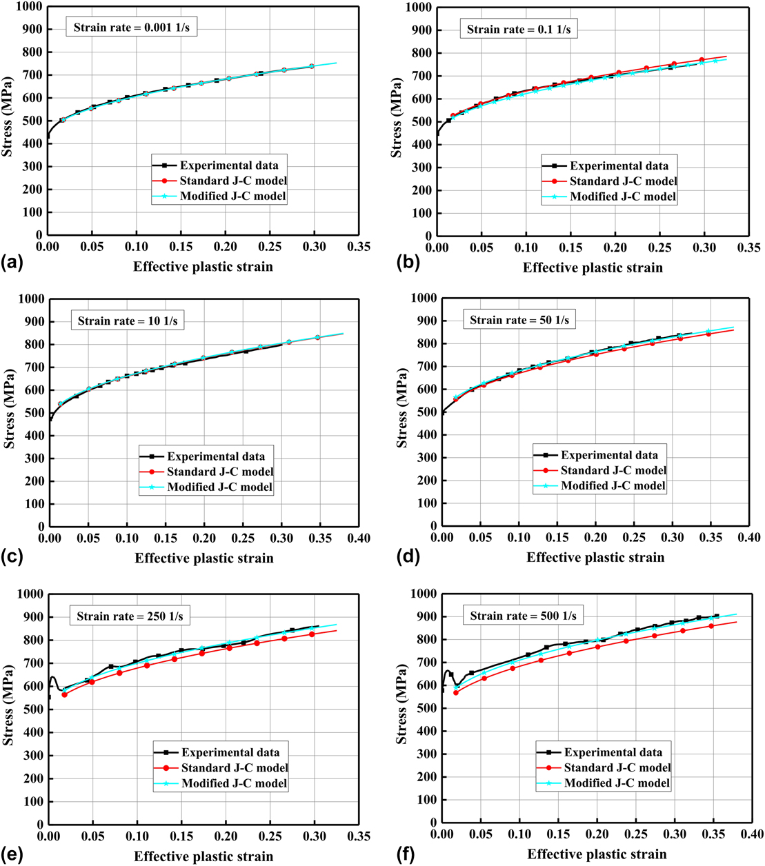
The fitting curves obtained by the standard J–C model were compared with the experimental results for the HC420LA steel, as shown in Fig. 4. The error between the standard fitting curve and the experimental data was large. Thus, the parameters in the middle term of the constitutive model needed to be corrected. As shown in Fig. 3, true stress and logarithmic strain rate were approximated as power function. Considering that the standard J–C model described true stress and logarithmic strain rate as having a linear relationship, it was necessary to correct the strain rate strengthening items. Introducing parameter P, Eq. (1) translates into:
 $$\sigma = \left( {A + B{\varepsilon ^n}} \right)\left( {1 + C{{\left( {\ln {{\dot{\varepsilon }} \over {{{\dot{\varepsilon }}_0}}}} \right)}^P}} \right)\quad .$$
Comparison of the modified J–C model and standard J–C model predictions with experimental results for HC420LA steel: (a) strain rate = 0.001 s−1, (b) strain rate = 0.1 s−1, (c) strain rate = 10 s−1, (d) strain rate = 50 s−1, (e) strain rate = 250 s−1, and (f) strain rate = 500 s−1.

Rearranging Eq. (2) and taking natural logarithm on both sides, the following form was obtained:
 $$\ln \left( {{\sigma \over {A + B{\varepsilon ^n}}} - 1} \right) = \ln C + P\ln \left( {\ln {{\dot{\varepsilon }} \over {{{\dot{\varepsilon }}_0}}}} \right)\quad ,$$
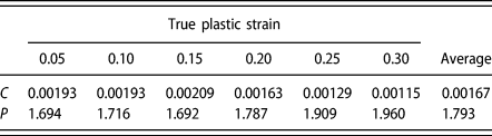
where C and P were determined by curve fitting, and the average values of C and P were calculated from six reference plastic strains, as given in Table II. The parameters of the modified J–C model are listed in Table III.
Strain-rate-sensitive parameters’ fitting results.

Parameters of the modified Johnson–Cook model for the HC420LA steel.

The curves obtained using the modified J–C model were compared with the stress–strain curves experimentally obtained in Fig. 4, which showed that the modified J–C model showed better agreement with the experimental data.
To visually reflect the correlation between the two models and the experimental data, the two models were evaluated using standard statistical parameters: correlation coefficient (R), average absolute relative error (AARE), and average root mean square error (RMSE), which were expressed as follows:
 $$R = {{\sum\limits_{i = 1}^{i = N} {\left( {\sigma _{\rm{e}}^i - \overline {{\sigma _{\rm{e}}}} } \right)\left( {\sigma _{\rm{p}}^i - \overline {{\sigma _{\rm{p}}}} } \right)} } \over {\sqrt {\sum\limits_{i = 1}^{i = N} {{{\left( {\sigma _{\rm{e}}^i - \overline {{\sigma _{\rm{e}}}} } \right)}^2}} \sum\limits_{i = 1}^{i = N} {{{\left( {\sigma _{\rm{p}}^i - \overline {{\sigma _{\rm{p}}}} } \right)}^2}} } }}\quad ,$$
 $${\rm{AARE}} = {1 \over N}\sum\limits_{i = 1}^{i = N} {\left| {{{\sigma _{\rm{e}}^i - \sigma _{\rm{p}}^i} \over {\sigma _{\rm{e}}^i}}} \right|} \times 100\% \quad ,$$
 $${\rm{RMSE}} = \sqrt {{1 \over N}\sum\limits_{i = 1}^{i = N} {{{\left( {\sigma _{\rm{e}}^i - \sigma _{\rm{p}}^i} \right)}^2}} } \quad ,$$
where σe and σp are experimental true stress and predicted true stress calculated by employing the corresponding model, respectively;  $\overline {{\sigma _{\rm{e}}}}$ and
 $\overline {{\sigma _{\rm{p}}}}$ are the average values of experimental true stress and predicted true stress, respectively; and parameter N is the amount of experimental true stress data used in the process of determining model parameters.
R presented the degree of linear correlation between the experimental data and predicted values. Because the two models differed only in the linear magnification factor, the values of R of two models at the same strain rate were exactly the same. After calculation, the values of R at six strain rates were greater than 0.98. This indicated that the predicted values of two models had a good linear correlation with the experimental data. AARE and RMSE used in this study were calculated through a term-by-term comparison of the relative error and therefore were unbiased statistical parameters for verifying the predictability of models [Reference Sabokpa, Zarei-Hanzaki, Abedi and Haghdadi24]. Comparison of the relative errors between predicted values obtained from the two models and the experimental data is shown in Supplementary material Fig. S1. AARE of the predicted values of the revised J–C model and standard J–C model were 0.889%–1.726% and 0.952%–4.277%, respectively. The average root mean square error of the predicted values of the revised J–C model and standard J–C model were 6.969–14.216 and 8.287–32.195, respectively. The error of the modified J–C model was significantly lower than that of the standard J–C model. Therefore, the modified J–C model could accurately describe the constitutive response of the HC420LA steel.
Validation of the numerical model
To verify the accuracy of the material model, dynamic tensile test at strain rate 100 s−1 was performed. Experimental results and comparison with the modified J–C model are shown in Supplementary material Fig. S2, which showed that the modified J–C model was in good agreement with the experimental data.
A 3D finite element model of the representative testing of HC420LA steel at a strain rate of 100 s−1 was defined in the FE code LS-DYNA 971. Eight-node 3D brick elements were applied in the total dynamic testing sample. An element size of 0.5 mm × 0.5 mm × 0.25 mm was selected in the gauge section for representing strain localization, and the model of the gauge section in the tensile specimen generated 6000 solid elements, as shown in Supplementary material Fig. S3. A speed boundary condition was implemented on the upper surface in the tensile specimen. Meanwhile, the modified J–C model (*MAT_15) was applied in finite element simulation. Furthermore, the fracture failure strain of the material in the numerical simulation was set to 0.69, which was determined using DIC method.
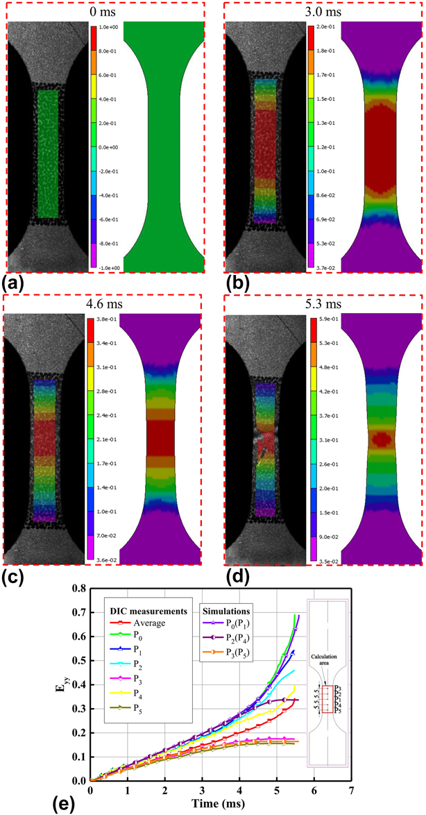
E yy field distribution and E yy–time curves of the calculation area from DIC measurement were compared with those from the numerical simulation, as shown in Fig. 5. The strain distributions of the calculation area were well matched. E yy (P 0) of the numerical simulation showed good consistency with DIC measurement. In the numerical simulation, the fracture occurred in the center of the specimen and was perpendicular to the tensile axis. Meanwhile, the strain distribution was symmetrical relative to the center of the specimen, so the strain of P 0 and P 1, P 2 and P 4, P 3, and P 5 was the same curve for the numerical simulation. The strain of other reference points of DIC measurement was slightly deviated when compared with numerical simulations because the fracture did not occur in the center of the specimen during the experiment. These results confirmed the rationality of using the modified J–C model and parameters of expression for numerical simulation.
Comparison of E yy field distribution and E yy–time curves of the calculation area from DIC measurements and numerical simulation at strain rate 100 s−1: (a) t = 0 ms, (b) t = 3.0 ms, (c) t = 4.6 ms, (d) t = 5.3 ms, and (e) E yy–time curves.

Conclusion
The tensile properties of the high-strength low-alloy (HC420LA) steel at a wide range of strain rates (0.001–500 s−1) under uniaxial tensile loads were investigated in this study. E yy response of the point near the fracture crack was larger than the average E yy of the whole selected calculation area due to strain localization. Based on experimental results, it could be determined that HC420LA steel had positive strain rate sensitivity in terms of the ultimate tensile stress, yield stress, and total elongation.
To characterize the strain-rate-dependent constitutive behavior of the investigated steel, a modified J–C model was used and model parameters were determined using experimental results. Predictions of the modified and standard J–C models were compared using standard statistical parameters, such as correlation coefficient, AARE, and average root mean square error, and the modified J–C model achieved a better agreement with the experimental data.
The typical test on HC420LA steel at a strain rate of 100 s−1 was modeled using the FE code LS-DYNA 971. The modified J–C model (*MAT_15) and the fracture strain obtained using DIC technique were applied in the finite element simulation. Good correlation between the experimental results and numerical simulation results was observed in terms of the strain response and strain field distribution of gauge region in tensile sample.
Experimental materials and methods
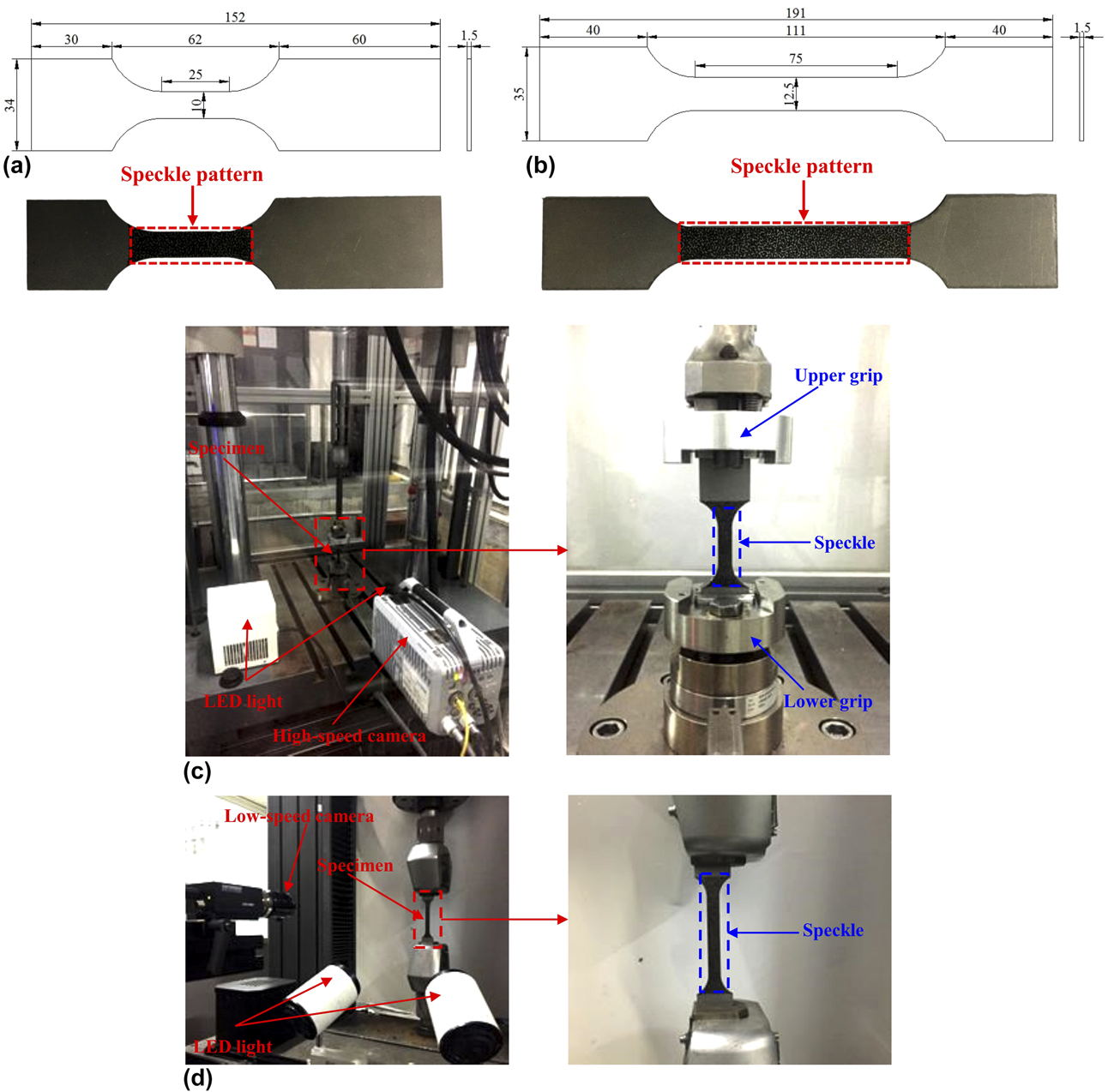
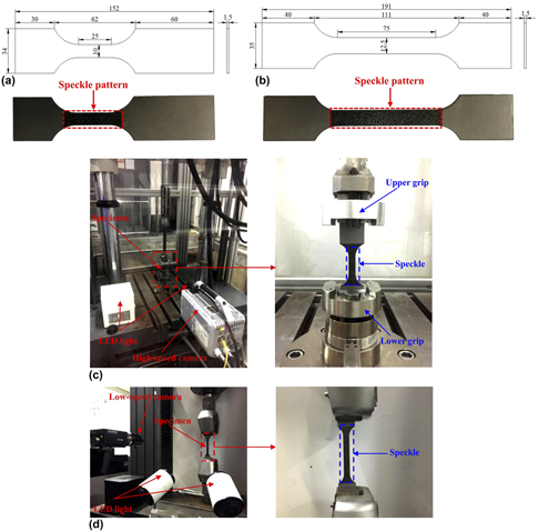
Chemical composition of the high-strength low-alloy (HC420LA) steel is given in Table IV. For high-strain-rate tensile experiments, specimen geometry was chosen with a parallel length of 25 mm, gauge length of 20 mm, width of 10 mm, and thickness of 1.5 mm, as shown in Fig. 6(a). The size of the specimens used for low-strain-rate tensile experiments is shown in Fig. 6(b). Its parallel length, gauge length, width, and thickness were 70 mm, 50 mm, 12.5 mm, and 1.5 mm, respectively. DIC technique combined with high-speed photography was used in evaluating the axial strain of parallel length through tracking the speckles attached to the sample surface. Therefore, the suitable speckles were sprayed on the parallel length surface of the experimental sample at random, as shown in Fig. 6.
Chemical composition of the investigated steel (in wt%).

Tensile specimen geometry (unit: mm) and the tested specimens with speckles: (a) at high strain rates and (b) at low strain rates; experimental setup: (c) high-speed tensile test and (d) low-strain-rate test.

A high-speed testing machine (Zwick/Roell HTM 5020 with the maximum impact load 50 kN and maximum tensile speed 20 m/s, ZwickRoell, Ulm, Germany) was used for high-strain-rate tensile experiments, as shown in Fig. 6(c). Meanwhile, a Photron FASTCAMSA-X2 high-speed camera (Imagica Group, Tokyo, Japan) was used to record the entire deformation processes of the tensile specimen. After fixing specimens, the communication between the high-speed tensile machine and the DIC cameras was established. Each time the DIC camera took a picture, the force sensor collected one load data. Experiments were performed at a constant speed. Four strain rates, 10, 50, 250, and 500 s−1, were chosen for high-strain-rate tensile tests. Responding tensile velocities were determined by the gauge length of the specimens and the strain rates. As a noncontacting full-field strain optical measurement method, DIC calculated the strain field of the deformed gauge region in the test specimen by comparing the reference picture recorded before loading with the subsequent pictures at different states. DIC analyzed the data in the photographs of testing specimens during the tensile process by pixels. So focal distance, resolution, and frame rate of the DIC high-speed camera were gradually adjusted to guarantee the images were clear. At strain rates 10, 50, 250, and 500 s−1, the frame rate was 12,500, 20,000, 81,000, and 112,500 fps, respectively, and resolution was 1024 × 1024, 256 × 568, 128 × 568, and 128 × 376 pixels, respectively. Low-strain-rate tensile experiments (0.001, 0.1 s−1) were performed using a universal testing machine (Instron 5985, Instron, Boston, Massachusetts) which could bear the maximum load of 150 kN, as shown in Fig. 6(d). A DIC low-speed camera was used to record the entire failure process. For both quasi-static and dynamic experiments, three specimens were tested at the same strain rate.
Supplementary material
To view supplementary material for this article, please visit https://doi.org/10.1557/jmr.2018.439.
Data availability
The raw/processed data required to reproduce these findings cannot be shared at this time due to technical or time limitations.
Acknowledgment
This project is supported by The National Key Research and Development Program of Hunan Province (2017GK2090).