2.1 Stably stratified shear layers with uniform stratification

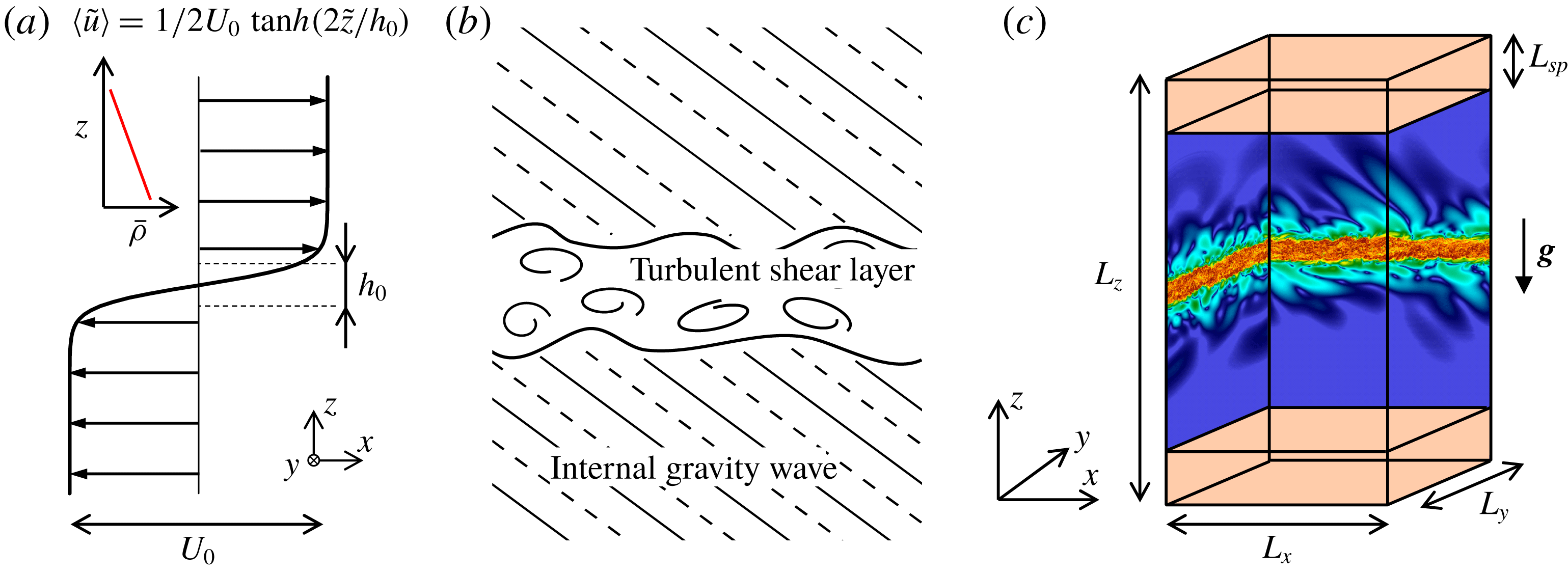
The problem considered here is a temporally evolving shear layer in a uniformly stratified fluid as shown in figure 1. The coordinates $x$ , $y$ and $z$ are in the streamwise, spanwise and vertical directions, respectively. The initial mean velocity profile is given by $\langle \tilde{u} \rangle =0.5U_{0}\,\text{tanh}(2\tilde{z}/h_{0})$ , where $U_{0}$ and $h_{0}$ are the initial velocity difference and the initial vorticity thickness, respectively. Here, the tilde represents the dimensional variables. The shear layer develops in a stably stratified fluid with a constant background density gradient in the vertical direction $\text{d}\overline{\unicode[STIX]{x1D70C}}/\text{d}z$ , where the roller vortices of the KH instability and the turbulence can excite internal gravity waves outside the shear layer. The buoyancy frequency $N_{b}$ for the background density gradient is defined as $N_{b}^{2}=-(g/\unicode[STIX]{x1D70C}_{0})(\text{d}\overline{\unicode[STIX]{x1D70C}}/\text{d}z)$ with a constant reference density $\unicode[STIX]{x1D70C}_{0}$ and the gravitational acceleration $g$ . The flow is characterized by three non-dimensional parameters, i.e. the Reynolds number $Re$ , Prandtl number $Pr$ and Froude number $Fr$ , defined as follows

(2.1a-c ) $$\begin{eqnarray}\displaystyle & \displaystyle Re={\displaystyle \frac{U_{0}h_{0}}{\unicode[STIX]{x1D708}}},\quad Pr={\displaystyle \frac{\unicode[STIX]{x1D708}}{\unicode[STIX]{x1D705}}},\quad Fr={\displaystyle \frac{2U_{0}}{h_{0}N_{b}}}, & \displaystyle\end{eqnarray}$$

where $\unicode[STIX]{x1D708}$ is the kinematic viscosity and $\unicode[STIX]{x1D705}$ is the mass diffusivity. Non-dimensional variables are introduced as

(2.2a-e ) $$\begin{eqnarray}\displaystyle & \displaystyle x_{i}={\displaystyle \frac{\tilde{x}_{i}}{h_{0}}},\quad t={\displaystyle \frac{\tilde{t}}{h_{0}/U_{0}}},\quad u_{i}={\displaystyle \frac{\tilde{u} _{i}}{U_{0}}},\quad \unicode[STIX]{x1D70C}={\displaystyle \frac{\tilde{\unicode[STIX]{x1D70C}}}{h_{0}(-\text{d}\overline{\unicode[STIX]{x1D70C}}/\text{d}z)}},\quad p={\displaystyle \frac{\tilde{p}}{\unicode[STIX]{x1D70C}_{0}U_{0}^{2}}},\qquad & \displaystyle\end{eqnarray}$$

where $x_{i}$ , $t$ , $u_{i}$ , $\unicode[STIX]{x1D70C}$ and $p$ denote position, time, velocity, density and pressure, respectively. We employ the Boussinesq approximation, under which the governing equations are given in non-dimensional form as

(2.3) $$\begin{eqnarray}\displaystyle & \displaystyle {\displaystyle \frac{\unicode[STIX]{x2202}u_{i}}{\unicode[STIX]{x2202}x_{i}}}=0, & \displaystyle\end{eqnarray}$$

(2.4) $$\begin{eqnarray}\displaystyle & \displaystyle {\displaystyle \frac{\unicode[STIX]{x2202}u_{i}}{\unicode[STIX]{x2202}t}}+{\displaystyle \frac{\unicode[STIX]{x2202}u_{i}u_{j}}{\unicode[STIX]{x2202}x_{j}}}=-{\displaystyle \frac{\unicode[STIX]{x2202}p}{\unicode[STIX]{x2202}x_{i}}}+{\displaystyle \frac{1}{Re}}{\displaystyle \frac{\unicode[STIX]{x2202}^{2}u_{i}}{\unicode[STIX]{x2202}x_{j}\unicode[STIX]{x2202}x_{j}}}-{\displaystyle \frac{4}{Fr^{2}}}\unicode[STIX]{x1D70C}^{\prime }\unicode[STIX]{x1D6FF}_{i3}, & \displaystyle\end{eqnarray}$$

(2.5) $$\begin{eqnarray}\displaystyle & \displaystyle {\displaystyle \frac{\unicode[STIX]{x2202}\unicode[STIX]{x1D70C}}{\unicode[STIX]{x2202}t}}+{\displaystyle \frac{\unicode[STIX]{x2202}u_{j}\unicode[STIX]{x1D70C}}{\unicode[STIX]{x2202}x_{j}}}={\displaystyle \frac{1}{Re\,Pr}}{\displaystyle \frac{\unicode[STIX]{x2202}^{2}\unicode[STIX]{x1D70C}}{\unicode[STIX]{x2202}x_{j}\unicode[STIX]{x2202}x_{j}}}, & \displaystyle\end{eqnarray}$$

where $i,j=1,2,3$ denote indices that represent the directions $x$ , $y$ and $z$ , respectively, $\unicode[STIX]{x1D6FF}_{ij}$ is the Kronecker delta, $p$ is the perturbation of the pressure from a mean reference value in hydrostatic balance, while the density is decomposed into a linearly varying part $\overline{\unicode[STIX]{x1D70C}}(z)$ and the density perturbation $\unicode[STIX]{x1D70C}^{\prime }=\unicode[STIX]{x1D70C}-\overline{\unicode[STIX]{x1D70C}}(z)$ .

Figure 1.

Stably stratified shear layer developing in a uniformly stratified fluid. (a) Initial velocity profile. (b) Sketch of stably stratified shear layer, which is surrounded by internal gravity waves propagating into non-turbulent fluid. The lines outside the shear layer represent phase lines of internal gravity waves. (c) Computational domain in DNS. Sponge layers with a thickness of $L_{sp}$ are imposed near vertical boundaries.

2.2 Numerical methods and computational parameters

The governing equations are solved with the DNS code based on the fractional step method used in Watanabe et al. (Reference Watanabe, Riley and Nagata2016b ). The initial field is generated by superimposing velocity fluctuations onto the mean velocity profile, where the fluctuating components are obtained by a diffusion process (Kempf, Klein & Janicka Reference Kempf, Klein and Janicka2005). The initial density perturbation $\unicode[STIX]{x1D70C}^{\prime }$ is 0. The fourth-order and second-order fully conservative finite difference schemes (Morinishi et al. 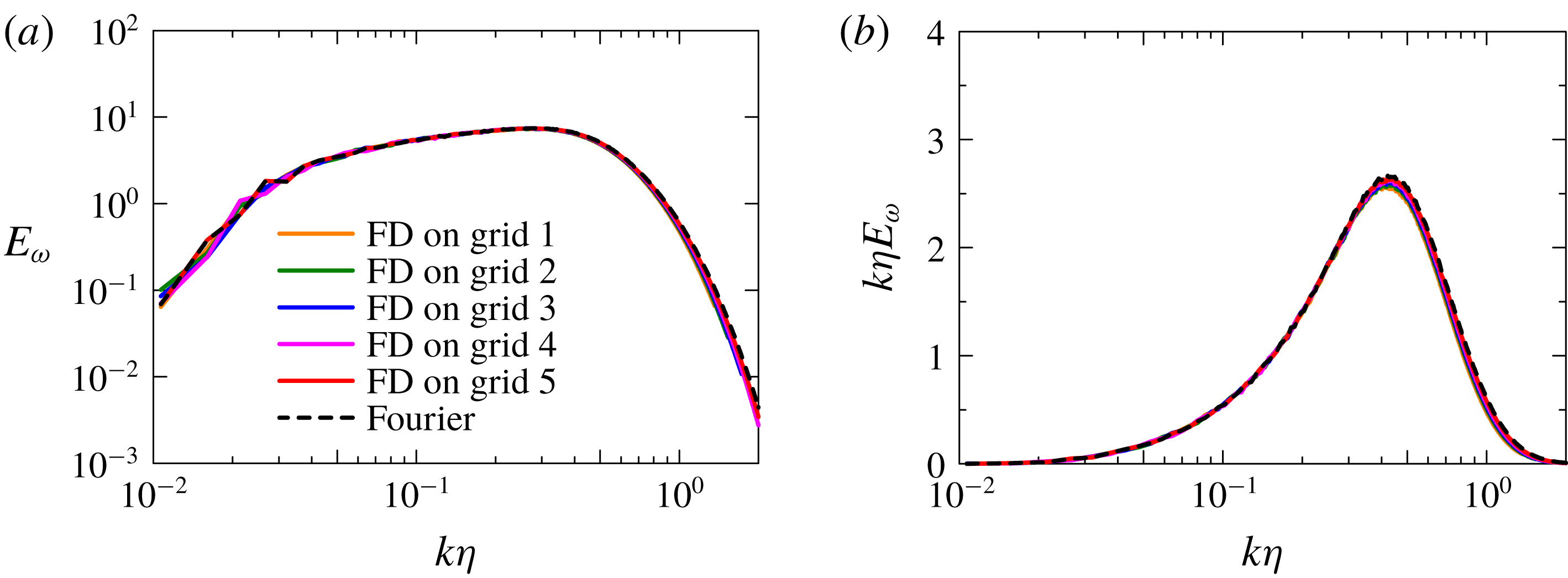Reference Morinishi, Lund, Vasilyev and Moin1998) are used on staggered grids for the spatial discretization in the horizontal directions and vertical direction, respectively, while the third-order Runge–Kutta method is employed for temporal advancement. An error in these fourth-order and second-order fully conservative finite difference schemes was quantified for first and second derivatives with Fourier analysis by Nagarajan, Lele & Ferziger (Reference Nagarajan, Lele and Ferziger2003) and Suzuki et al. (Reference Suzuki, Nagata, Sakai, Hayase, Hasegawa and Ushijima2013). Appendix A provides further examinations of these schemes based on a homogeneous isotropic velocity field with a prescribed spectrum. The Bi-CGSTAB method is used for solving the Poisson equation for pressure (Van der Vorst Reference Van der Vorst1992). DNS of non-stratified free shear flows (Watanabe et al. Reference Watanabe, Sakai, Nagata, Ito and Hayase2015) showed that the conditional statistics of enstrophy and its transport equation obtained with the present code are similar to those by the pseudo-spectral code used by Taveira & da Silva (Reference Taveira and da Silva2014).

The computational domain with the size of $(L_{x}\times L_{y}\times L_{z})=(42h_{0}\times 28h_{0}\times 80h_{0})$ is represented by $(N_{x}\times N_{y}\times N_{z})$ grid points. The grid spacing is uniform in the horizontal directions while the grid is stretched in the vertical direction near the vertical boundaries. We use the following mapping function that converts integer $k=1,\ldots ,N_{z}$ to the vertical location

(2.6) $$\begin{eqnarray}\displaystyle & \displaystyle z(k)=-{\displaystyle \frac{L_{z}}{2\unicode[STIX]{x1D6FC}_{z}}}\text{atanh}\left\{\!(\text{tanh}\,\unicode[STIX]{x1D6FC}_{z})\left[1-2\left({\displaystyle \frac{k-1}{N_{z}-1}}\right)\right]\right\}, & \displaystyle\end{eqnarray}$$

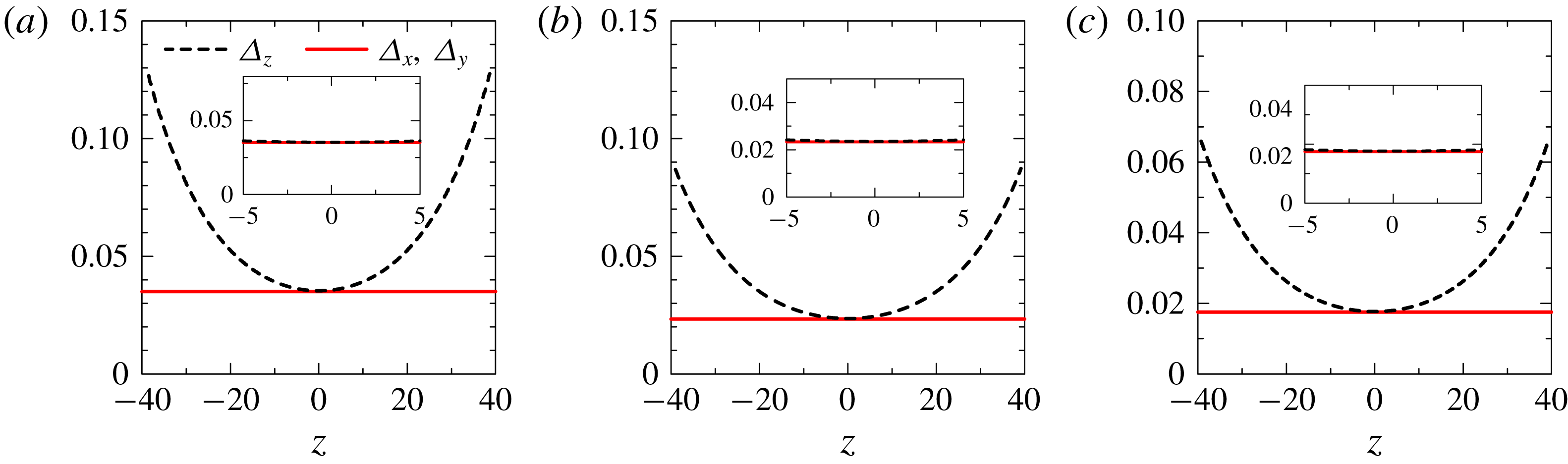
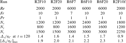
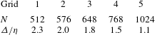
with $\unicode[STIX]{x1D6FC}_{z}=1.3$ . Periodic boundary conditions are used in the horizontal directions. Internal gravity waves are emitted outwards as the shear layer develops (figure 1(b)). The vertical boundaries are treated with free-slip boundary conditions with a sponge layer with the thickness $L_{sp}=10h_{0}$ , which prevents the reflections of internal gravity waves (Pham & Sarkar Reference Pham and Sarkar2010). The computational and flow parameters are summarized in table 1. We perform the DNS with two different grid settings for $(Re,Fr)=(2000,10)$ for checking the influence of the spatial resolution, where R2F10f with a finer grid is used for comparison with R2F10. Figure 2 shows vertical profiles of the grid size $\unicode[STIX]{x1D6E5}_{i}$ ( $i=x,~y$ or $z$ ). During the simulation, the turbulent shear layer develops for $|z|<5$ , where the grid size is almost the same in all directions. Note that the initial velocity fluctuations are slightly different between R2F10 and R2F10f because of different spatial resolutions. Because of sensitivity to initial perturbations, the resulting turbulent shear layer also shows slight differences. The DNS is performed until $t=200$ for R2F10f and until $t=300$ for the other cases. We analyse snapshots of the flow fields at $t=80$ , 120, 160, 200 and 240 for investigating the TNTI layer since the turbulent shear layer has reached a fully developed state before $t=80$ in the sense that the mean turbulent kinetic energy dissipation rate on the centreline peaks for $t<80$ . An average, denoted by $\langle ~\rangle$ , is taken in a horizontal plane as a function of $z$ . Table 1 also shows the grid size $\unicode[STIX]{x1D6E5}_{x}$ divided by the Kolmogorov length scale on the centreline, $\unicode[STIX]{x1D702}_{C}$ , at $t=120$ and at the instant with maximum $\unicode[STIX]{x1D6E5}_{x}/\unicode[STIX]{x1D702}_{C}$ , indicating that the grid is small enough to capture small-scale fluctuations.

Figure 2.

Vertical profiles of computational grid size $\unicode[STIX]{x1D6E5}_{i}$ : (a) R2F10 and R2F20; (b) R2F10f; and (c) R6F7, R6F10 and R6F10. The insets show $\unicode[STIX]{x1D6E5}_{i}$ for $-5\leqslant z\leqslant 5$ , where turbulent shear layers develop.

Table 1.

DNS dataset of stably stratified shear layers.

Figure 3.

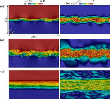
Streamwise velocity $u$ (left) and enstrophy $\unicode[STIX]{x1D714}_{i}\unicode[STIX]{x1D714}_{i}/2$ (right) on an $x$ – $z$ plane for R6F10 at (a) $t=40$ , (b) $t=80$ and (c) $t=200$ .

3.1 Temporal evolutions of stratified shear layers

Figure 3 shows streamwise velocity $u$ and enstrophy $\unicode[STIX]{x1D714}_{i}\unicode[STIX]{x1D714}_{i}/2$ on an $x$ – $z$ plane for run R6F10, where $\unicode[STIX]{x1D714}_{i}$ is the vorticity vector. In figure 3(a) one can see that the turbulence grows by the early time $t=40$ due to the KH instability. Small-scale turbulence exists in the entire shear layer at $t=80$ in figure 3(b), and the structures in the high-enstrophy regions are seen to be clearly different when comparing the results for $t=80$ and 200. The existence of internal gravity waves is clear from examining the enstrophy field outside the shear layer. Finally, the spatial distribution of vorticity in the internal wave region also evolves in time, as more waves and smaller-scale structures appear at later times.

The momentum thickness of the shear layer $\unicode[STIX]{x1D6FF}_{u}$ is defined by

(3.1) $$\begin{eqnarray}\displaystyle & \displaystyle \unicode[STIX]{x1D6FF}_{u}=\int _{-L_{z}/2}^{L_{z}/2}(0.5-\langle u\rangle )(0.5+\langle u\rangle )\,\text{d}z. & \displaystyle\end{eqnarray}$$

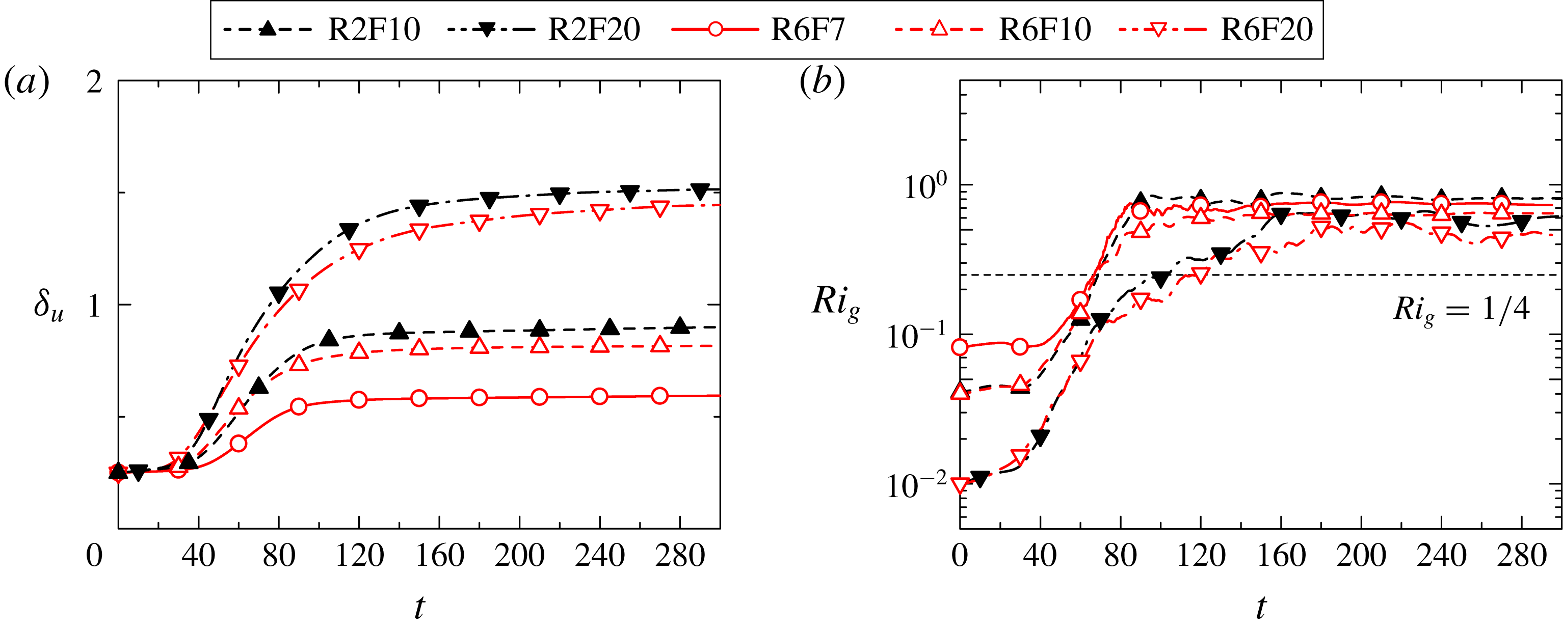
The temporal evolution of $\unicode[STIX]{x1D6FF}_{u}$ is shown in figure 4(a). As the turbulence grows due to the KH instability, $\unicode[STIX]{x1D6FF}_{u}$ begins to increase rapidly with time starting at approximately $t=40$ . This rapid growth continues out to a time that depends on the Froude number, and then $\unicode[STIX]{x1D6FF}_{u}$ ultimately almost ceases to grow. This cessation of growth occurs at approximately $t=100$ for the lowest Froude-number case (R6F7), and this time increases with Froude number and occur at approximately $t=140$ for the highest Froude-number cases (R2F20 and R6F20). Note that the extent of growth of $\unicode[STIX]{x1D6FF}_{u}$ also increases as the Froude number increases. This increase with the Froude number of $\unicode[STIX]{x1D6FF}_{u}$ and of the time to cessation of growth is expected, since the effect of stratification decreases as the Froude number is increased. Note also that the Reynolds numbers of these flows are high enough that the results only weakly depend on the Reynolds number.

Figure 4(b) shows the temporal evolution of the gradient Richardson number $Ri_{g}$ on the centreline, where $Ri_{g}$ is defined with the mean vertical gradient of streamwise velocity $\tilde{S}=\langle \unicode[STIX]{x2202}\tilde{u} /\unicode[STIX]{x2202}\tilde{z}\rangle$ and the buoyancy frequency ${\tilde{N}}=\sqrt{-(g/\unicode[STIX]{x1D70C}_{0})\langle \unicode[STIX]{x2202}\tilde{\unicode[STIX]{x1D70C}}/\unicode[STIX]{x2202}\tilde{z}\rangle }$ as

(3.2) $$\begin{eqnarray}\displaystyle & \displaystyle Ri_{g}={\displaystyle \frac{N^{2}}{S^{2}}}=-{\displaystyle \frac{g\langle \unicode[STIX]{x2202}\tilde{\unicode[STIX]{x1D70C}}/\unicode[STIX]{x2202}\tilde{z}\rangle }{\unicode[STIX]{x1D70C}_{0}\langle \unicode[STIX]{x2202}\tilde{u} /\unicode[STIX]{x2202}\tilde{z}\rangle ^{2}}}. & \displaystyle\end{eqnarray}$$

Here the total density gradient is used in (3.2). We find that $Ri_{g}$ also begins to increase rapidly approximately $t=40$ , and becomes independent of time and of the Froude number after the shear layer is well developed, although this comes later for the higher Froude-number cases. Also, for larger times $Ri_{g}$ exceeds $1/4$ , the critical value for shear instability (Hazel Reference Hazel1972).

Figure 4.

Temporal evolutions of (a) the momentum thickness $\unicode[STIX]{x1D6FF}_{u}$ and (b) the gradient Richardson number $Ri_{g}$ on the centreline.

Figure 5.

(a) Temporal evolution of buoyancy Reynolds number $Re_{b}$ on the centreline. (b) Plot of $Re_{b}$ against time normalized by background buoyancy frequency.

Figure 6.

Vertical profiles of (a) mean streamwise velocity $\langle u\rangle$ , (b) mean vertical gradient of total density $\unicode[STIX]{x2202}\langle \unicode[STIX]{x1D70C}\rangle /\unicode[STIX]{x2202}z$ , (c) r.m.s. streamwise velocity fluctuation $u_{rms}=\langle {u^{\prime }}^{2}\rangle ^{1/2}$ and (d) r.m.s. vertical velocity fluctuation $w_{rms}=\langle {w^{\prime }}^{2}\rangle ^{1/2}$ . The results are taken from run R6F10.

Another important non-dimensional number in the stratified shear layer is the buoyancy Reynolds number, which is defined with the ratio of Ozmidov scale $\tilde{L}_{O}=(\langle \tilde{\unicode[STIX]{x1D700}}\rangle /{\tilde{N}}^{3})^{1/2}$ to Kolmogorov scale $\tilde{\unicode[STIX]{x1D702}}=(\unicode[STIX]{x1D708}^{3}/\langle \tilde{\unicode[STIX]{x1D700}}\rangle )^{1/4}$  (here $\langle \tilde{\unicode[STIX]{x1D700}}\rangle =\langle 2\unicode[STIX]{x1D708}\tilde{\unicode[STIX]{x1D61A}}_{ij}\tilde{\unicode[STIX]{x1D61A}}_{ij}\rangle$ is the mean kinetic energy dissipation rate, and $\tilde{\unicode[STIX]{x1D61A}}_{ij}$ is the rate-of-strain tensor) as

(3.3) $$\begin{eqnarray}\displaystyle & \displaystyle Re_{b}=\left({\displaystyle \frac{\tilde{L}_{O}}{\tilde{\unicode[STIX]{x1D702}}}}\right)^{4/3}={\displaystyle \frac{\langle \tilde{\unicode[STIX]{x1D700}}\rangle }{\unicode[STIX]{x1D708}{\tilde{N}}^{2}}}. & \displaystyle\end{eqnarray}$$

This quantity is also called a turbulence intensity parameter in oceanography (Barry et al. Reference Barry, Ivey, Winters and Imberger2001; Shih et al. Reference Shih, Koseff, Ivey and Ferziger2005; de Lavergne et al. Reference de Lavergne, Madec, Le Sommer, Nurser and Naveira Garabato2016). It is argued that the scales larger than the Ozmidov scale are strongly affected by buoyancy. Thus, direct influences of buoyancy on small-scale turbulence are weak when $L_{O}\gg \unicode[STIX]{x1D702}$ or, equivalently, $Re_{b}\gg O(10^{0})$ . 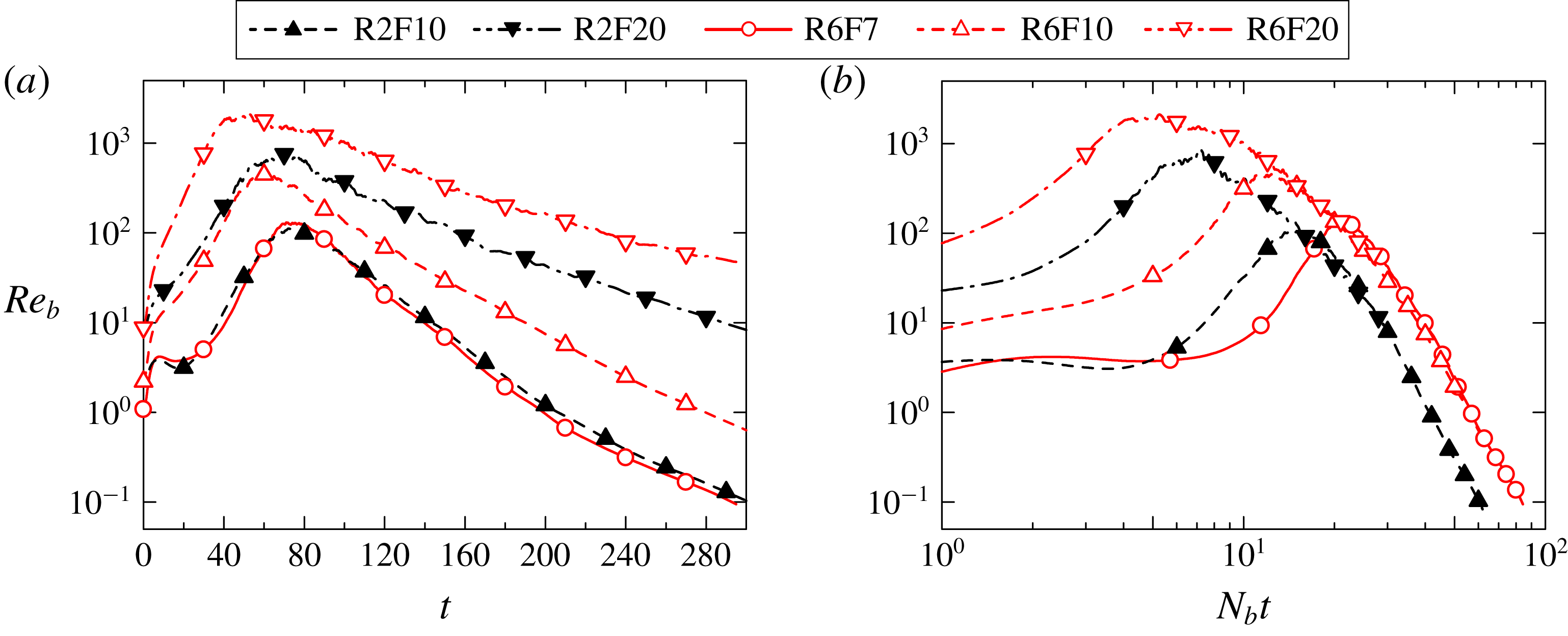Figure 5(a,b) show $Re_{b}$ on the centreline as a function of $t=\tilde{t}/(h_{0}/U_{0})$ and $N_{b}\tilde{t}$ , respectively. Initially $Re_{b}$ increases with time similarly to $Ri_{g}$ and reaches $O(10^{2})\sim O(10^{3})$ , which is large enough for small-scale turbulence to exist. As the turbulence decays with time, $Re_{b}$ also decreases. Except for the case R6F20, $Re_{b}$ becomes less than 10 during the simulation, indicating that the turbulence over all scales is influenced by buoyancy. When time is non-dimensionalized with the background buoyancy frequency $N_{b}$ as in figure 5(b), $Re_{b}$ tends to collapse onto a single curve independent of $Fr$ , but with a weak dependence on $Re$ . This may be related to the collapse of $Ri_{g}$ for larger time in figure 4(b).

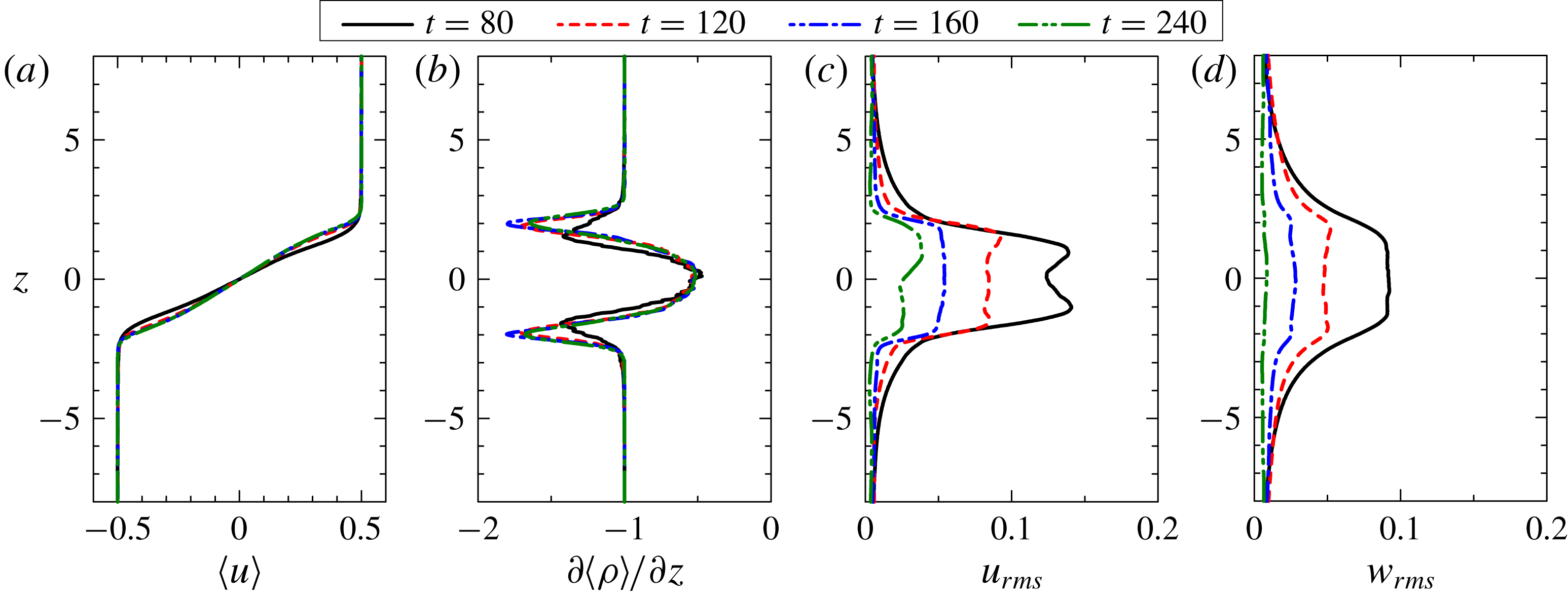
Figure 6 shows the vertical profiles of mean streamwise velocity $\langle u\rangle$ , vertical gradient of mean total density $\unicode[STIX]{x2202}\langle \unicode[STIX]{x1D70C}\rangle /\unicode[STIX]{x2202}z$ , and root-mean-square (r.m.s.) values of streamwise and vertical velocity fluctuations ( $u_{i}^{\prime }=u_{i}-\langle u_{i}\rangle$ ) at different times for run R6F10. From the mean velocity profile in figure 6(a), the shear layer can be seen to remain localized in the region $-2\leqslant z\leqslant 2$ . The mean density gradient $\unicode[STIX]{x2202}\langle \unicode[STIX]{x1D70C}\rangle /\unicode[STIX]{x2202}z$ has large negative values near the edges of the shear layer, indicating very stable layers, while $\unicode[STIX]{x2202}\langle \unicode[STIX]{x1D70C}\rangle /\unicode[STIX]{x2202}z$ in the centre region is smaller in magnitude than the external value ( $|z|\geqslant 2$ ), an indication of turbulent mixing in the interior. This behaviour is similar to the DNS results for a shear layer developing above a stably stratified region (Pham & Sarkar Reference Pham and Sarkar2010). A difference between the present DNS and Pham & Sarkar (Reference Pham and Sarkar2010) is that a background density gradient is uniform in the vertical direction in this study whereas Pham et al. (Reference Pham, Sarkar and Brucker2009) considered the density gradient varying in the vertical direction, where the turbulent shear layer develops under a relatively weak influence of the stable stratification compared with the outside. In figure 6(c,d), both the horizontal and vertical velocity fluctuations are found to decrease with time. The horizontal velocity fluctuations are consistently larger than the corresponding vertical ones. At $t=240$ , the vertical r.m.s. velocity near the centreline is comparable to the value outside the shear layer, as the stratification suppresses the vertical motion in the shear layer and the velocity fluctuations are induced by the internal gravity waves outside the shear layer.

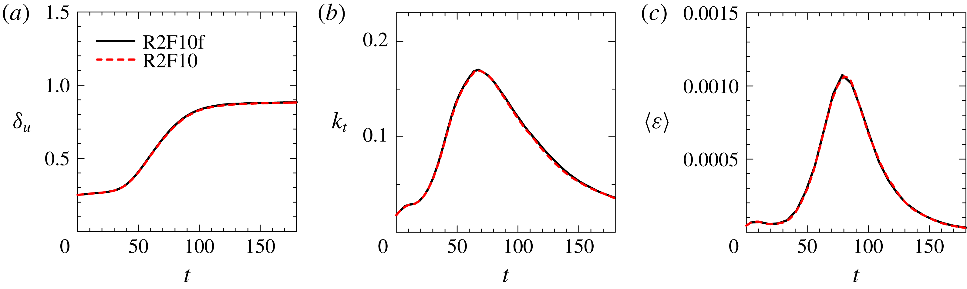
Figure 7 compares the temporal evolution of $\unicode[STIX]{x1D6FF}_{u}$ , the turbulent kinetic energy $k_{t}=\langle {u^{\prime }}^{2}+{v^{\prime }}^{2}+{w^{\prime }}^{2}\rangle /2$ and the mean kinetic energy dissipation rate $\langle \unicode[STIX]{x1D700}\rangle$ between R2F10 and R2F10f. These plots are almost identical for these simulations, where R2F10f has a higher resolution than R2F10, as shown in table 1.

Figure 7.

Temporal evolutions of (a) the momentum thickness $\unicode[STIX]{x1D6FF}_{u}$ , (b) the turbulent kinetic energy $k_{t}=\langle {u^{\prime }}^{2}+{v^{\prime }}^{2}+{w^{\prime }}^{2}\rangle /2$ and (c) the mean kinetic energy dissipation rate $\langle \unicode[STIX]{x1D700}\rangle$ on the centreline in runs R2F10 and R2F10f.

3.2 Detection of the turbulent region

In non-stratified free shear flows, an important characteristic of turbulent flow is its strong vorticity, and this property can be used to define and detect turbulent regions in a flow (e.g. Corrsin & Kistler Reference Corrsin and Kistler1955). In the present DNS the flow outside the shear layer contains internal waves which propagate outwards from the shear layer as in figure 3; these internal waves possess vorticity, but not other properties of turbulence, such as strong mixing and strong dissipation rates, and so should not be characterized as turbulence. The internal waves, however, contain no potential vorticity $\unicode[STIX]{x1D6F1}=\unicode[STIX]{x1D74E}\boldsymbol{\cdot }\unicode[STIX]{x1D735}\unicode[STIX]{x1D70C}$ , which is not directly affected by the buoyancy, so that it can be used for identifying the turbulent region following Watanabe et al. (Reference Watanabe, Riley, de Bruyn Kops, Diamessis and Zhou2016a ). We refer to a fluid with $|\unicode[STIX]{x1D6F1}|$ larger than a certain threshold $\unicode[STIX]{x1D6F1}_{th}$ as a turbulent fluid. 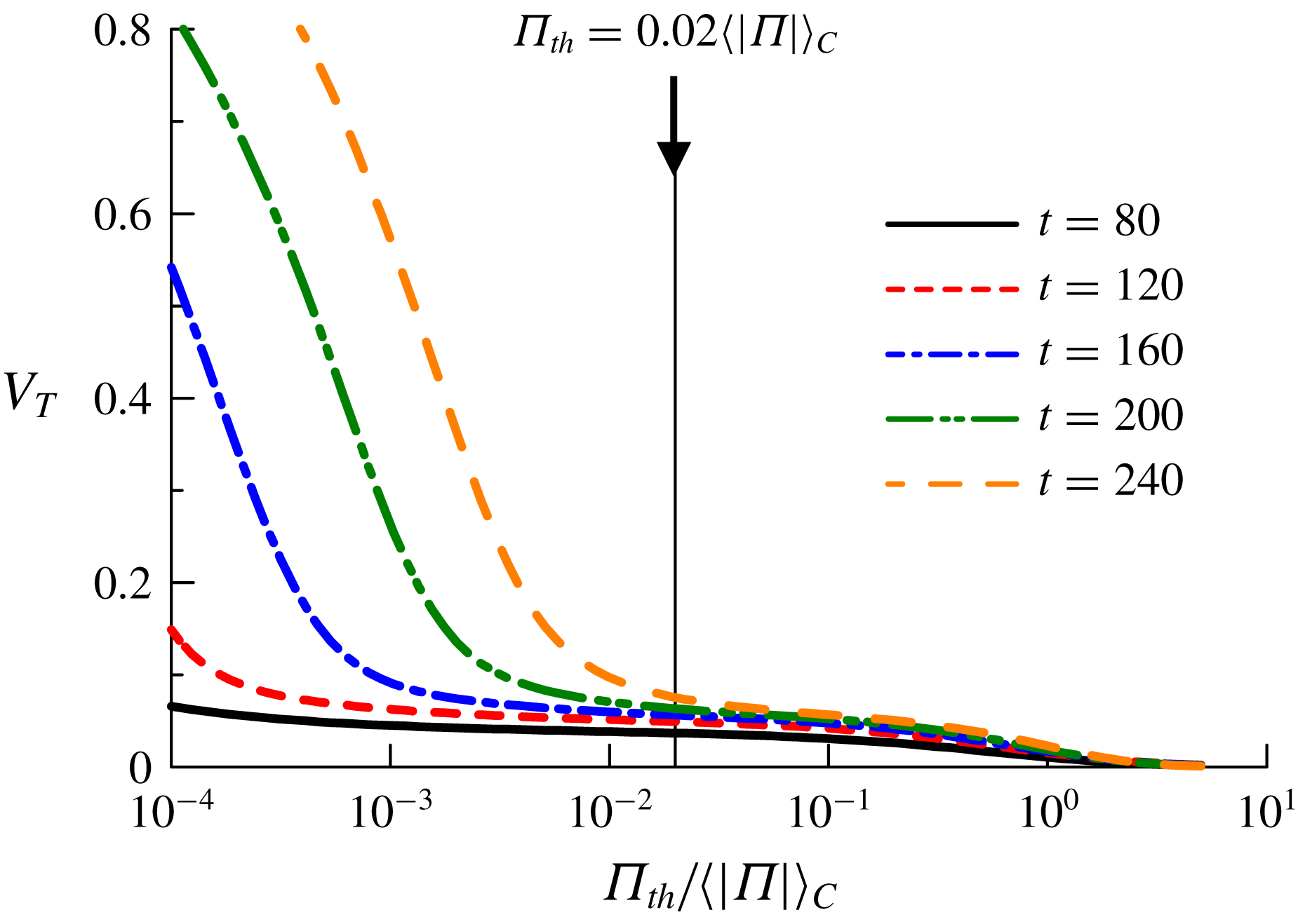When the level of $|\unicode[STIX]{x1D6F1}|$ is very different between turbulent and non-turbulent fluids, the volume fraction of the turbulent fluid $V_{T}$ in the computational domain only depends very weakly on $\unicode[STIX]{x1D6F1}_{th}$ for a wide range of $\unicode[STIX]{x1D6F1}_{th}$ (Taveira et al. Reference Taveira, Diogo, Lopes and da Silva2013). Figure 8 plots $V_{T}$ as a function of $\unicode[STIX]{x1D6F1}_{th}$ from $t=80$ to 240 for the case R6F10. The plots of $V_{T}$ are similar to those obtained in non-stratified planar jets, where enstrophy was used for detecting the turbulent region (Taveira et al. Reference Taveira, Diogo, Lopes and da Silva2013). The dependence of $V_{T}$ on $\unicode[STIX]{x1D6F1}_{th}$ is very weak for a certain range of $\unicode[STIX]{x1D6F1}_{th}$ , from which the threshold is chosen in the present study. Specifically, we use the value of $\unicode[STIX]{x1D6F1}_{th}=0.02\langle |\unicode[STIX]{x1D6F1}|\rangle _{C}$ , where $\langle |\unicode[STIX]{x1D6F1}|\rangle _{C}$ is the mean potential vorticity magnitude on the centreline. The same threshold $\unicode[STIX]{x1D6F1}_{th}=0.02\langle |\unicode[STIX]{x1D6F1}|\rangle _{C}$ is used in the other cases because the dependence of $V_{T}$ is similar. Previous studies on the TNTI have shown that a small change in the threshold determined from the turbulent volume hardly affects the location of the isosurface and the conditional statistics computed on the local interface coordinate (Taveira et al. Reference Taveira, Diogo, Lopes and da Silva2013; Watanabe, Zhang & Nagata Reference Watanabe, Zhang and Nagata2018).

Figure 8.

Volume fraction of turbulent fluid, $V_{T}$ , defined as a fluid with $|\unicode[STIX]{x1D6F1}|>\unicode[STIX]{x1D6F1}_{th}$ , plotted as a function of $\unicode[STIX]{x1D6F1}_{th}$ normalized by mean potential vorticity magnitude on the centreline $\langle |\unicode[STIX]{x1D6F1}|\rangle _{C}$ .

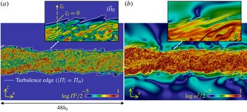
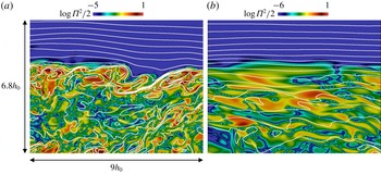
The outer edge of the turbulent region can be obtained as an isosurface of $|\unicode[STIX]{x1D6F1}|=\unicode[STIX]{x1D6F1}_{th}$ once the turbulent and non-turbulent fluids are detected. We refer to the isosurface of $|\unicode[STIX]{x1D6F1}|=\unicode[STIX]{x1D6F1}_{th}$ hereafter as the turbulence edge. The layer through which the flow changes from non-turbulent to turbulent, and the potential vorticity increases rapidly, is a layer with a finite thickness, which is called the TNTI layer in this paper. Figure 9 shows the instantaneous profiles of potential enstrophy $\unicode[STIX]{x1D6F1}^{2}/2$ and enstrophy $\unicode[STIX]{x1D714}^{2}/2$ with the turbulence edge on a $x$ – $z$ plane. We find that the isosurface $|\unicode[STIX]{x1D6F1}|=\unicode[STIX]{x1D6F1}_{th}$ successfully detects the outer edge of the turbulent region defined in terms of potential vorticity. The non-turbulent region possesses a significant level of enstrophy, as seen in figure 9(b). The structure of the enstrophy is, however, very different between the turbulent and non-turbulent regions: the smaller-scale structures can be observed in the turbulent region.

Figure 9.

Visualizations of both (a) potential enstrophy $\unicode[STIX]{x1D6F1}^{2}/2$ and (b) enstrophy $\unicode[STIX]{x1D714}^{2}/2$ at $t=120$ in R6F10. The turbulence edge detected as $|\unicode[STIX]{x1D6F1}|=\unicode[STIX]{x1D6F1}_{th}$ is indicated by white lines. Panel (a) also defines a local interface coordinate used for analysing statistics near the turbulence edge.

We use the conditional statistics computed as a function of distance from the turbulence edge (Bisset et al. Reference Bisset, Hunt and Rogers2002). The local coordinate with the origin at the turbulence edge, $\unicode[STIX]{x1D701}_{I}$ , is defined in the inset of figure 9(a). This $\unicode[STIX]{x1D701}_{I}$ is taken in the vertical outward direction, where the turbulent region is represented by negative $\unicode[STIX]{x1D701}_{I}$ . We denote the average taken as a function of $\unicode[STIX]{x1D701}_{I}$ as $\langle ~\rangle _{I}$ . We present the conditional statistics as a function of $\unicode[STIX]{x1D701}_{I}$ normalized by the Kolmogorov scale on the centreline $\unicode[STIX]{x1D702}_{C}$ . The conditional statistics are computed for the upper side of the shear layer. The TNTI layer in the lower side is also used for the conditional statistics by changing the sign of the relevant quantities, since the flow is statistically antisymmetric.

Figure 10.

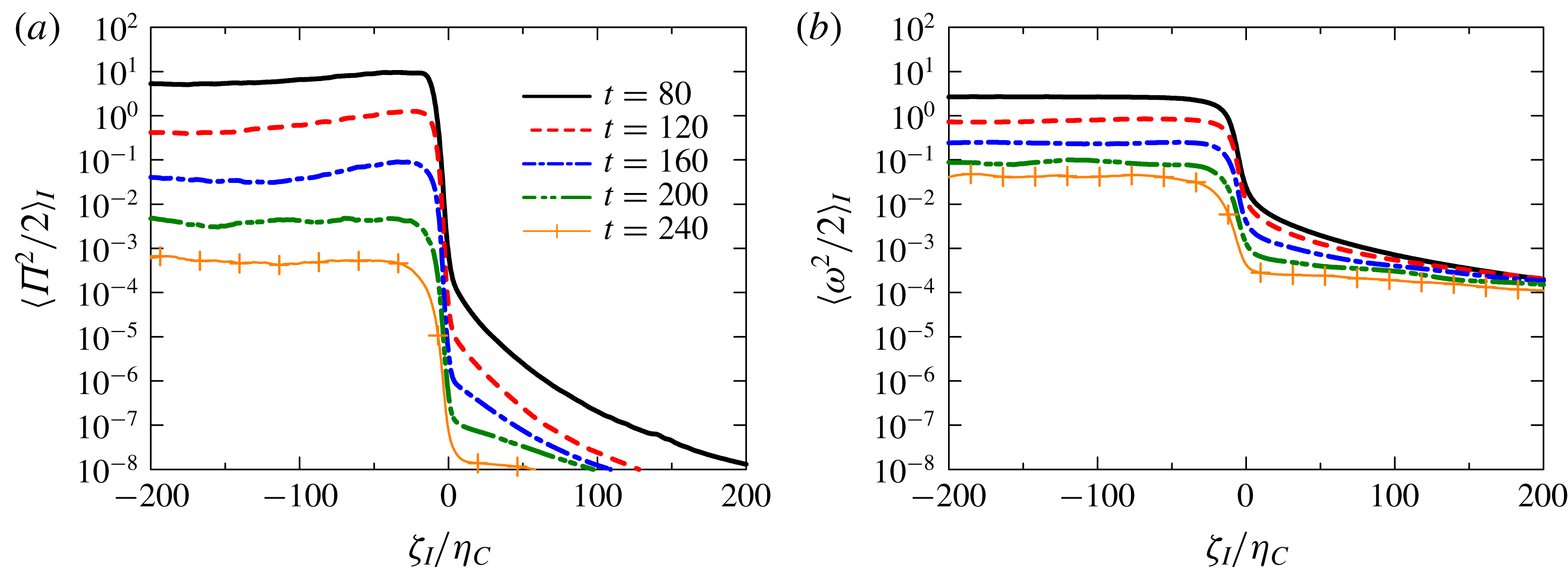
Conditional averages of both (a) potential enstrophy and (b) enstrophy in R6F10. The distance from the turbulence edge, $\unicode[STIX]{x1D701}_{I}$ , is normalized by Kolmogorov scale on the centreline $\unicode[STIX]{x1D702}_{C}$ .

Figure 11.

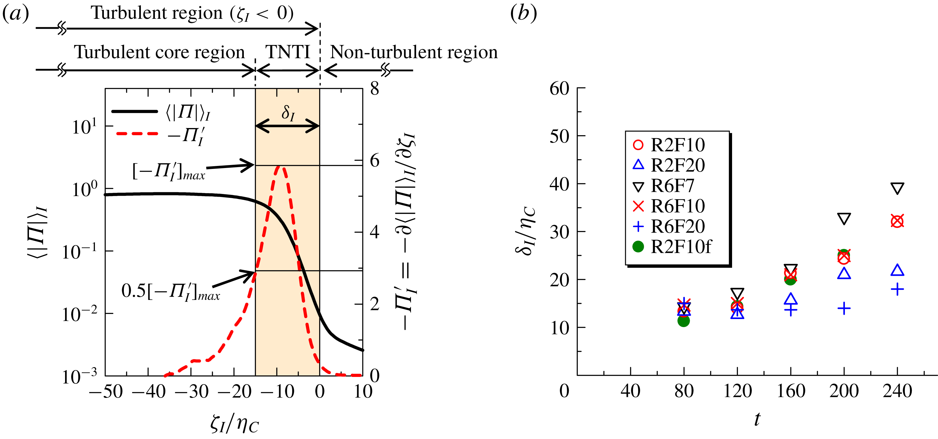
Mean thickness of the TNTI layer. (a) Estimation of the TNTI layer thickness based on the conditional mean potential vorticity magnitude. (b) Temporal evolution of the normalized thickness $\unicode[STIX]{x1D6FF}_{I}/\unicode[STIX]{x1D702}_{C}$ .

3.3 Enstrophy and potential enstrophy near the interface

Figure 10 shows the conditional averages of potential enstrophy and enstrophy, ( $\langle \unicode[STIX]{x1D6F1}^{2}/2\rangle _{I}$ and $\langle \unicode[STIX]{x1D714}^{2}/2\rangle _{I}$ ), at different times for R6F10. It can be seen that $\langle \unicode[STIX]{x1D6F1}^{2}/2\rangle _{I}$ decreases sharply from the turbulent to the non-turbulent region. The difference in $\langle \unicode[STIX]{x1D714}^{2}/2\rangle _{I}$ between the turbulent and non-turbulent regions is smaller than that in $\langle \unicode[STIX]{x1D6F1}^{2}/2\rangle _{I}$ , although $\langle \unicode[STIX]{x1D714}^{2}/2\rangle _{I}$ also decreases sharply. Similar plots were obtained in stratified wakes (Watanabe et al. Reference Watanabe, Riley, de Bruyn Kops, Diamessis and Zhou2016a ). The enstrophy in the non-turbulent region is due to internal gravity waves, as visualized in figure 9(b).

The TNTI layer is where potential vorticity magnitude changes rapidly between the turbulent and non-turbulent regions. Therefore, we identify the TNTI layer as the region with large $\unicode[STIX]{x1D6F1}_{I}^{\prime }=\unicode[STIX]{x2202}\langle |\unicode[STIX]{x1D6F1}|\rangle _{I}/\unicode[STIX]{x2202}\unicode[STIX]{x1D701}_{I}$ . Figure 11(a) shows $-\unicode[STIX]{x1D6F1}_{I}^{\prime }$ in comparison with $\langle |\unicode[STIX]{x1D6F1}|\rangle _{I}$ , where the mean thickness of the TNTI layer is defined with a peak value of $-\unicode[STIX]{x1D6F1}_{I}^{\prime }$ denoted by $[-\unicode[STIX]{x1D6F1}_{I}^{\prime }]_{max}$ . We can use the turbulence edge located at $\unicode[STIX]{x1D701}_{I}=0$ as the outer edge of the TNTI layer. Then, the thickness $\unicode[STIX]{x1D6FF}_{I}$ is defined as the distance from $\unicode[STIX]{x1D701}_{I}=0$ to the location of $-\unicode[STIX]{x2202}\langle |\unicode[STIX]{x1D6F1}|\rangle _{I}/\unicode[STIX]{x2202}\unicode[STIX]{x1D701}_{I}=0.5[-\unicode[STIX]{x1D6F1}_{I}^{\prime }]_{max}$ after the peak, as in figure 11(a). It should be noted that the present method gives an estimation of the mean thickness since it is difficult to define the exact location of the inner edge of the TNTI layer from the conditional statistics. The thickness obtained in this way is plotted against $t$ in figure 11(b), where $\unicode[STIX]{x1D6FF}_{I}$ is normalized by the Kolmogorov scale on the centreline $\unicode[STIX]{x1D702}_{C}$ . We find that $\unicode[STIX]{x1D6FF}_{I}\approx 13\unicode[STIX]{x1D702}_{C}$ for early times ( $t=80$ and 120) in all cases. This value $13\unicode[STIX]{x1D702}_{C}$ is very close to the thickness estimated with the conditional enstrophy profile in non-stratified free shear flows (Watanabe, Nagata & da Silva Reference Watanabe, Nagata and da Silva2017b ). The $\unicode[STIX]{x1D6FF}_{I}/\unicode[STIX]{x1D702}_{C}$ value increases with time for $t>120$ , becoming larger than the TNTI layer thickness in non-stratified flows; note that in this range $\unicode[STIX]{x1D6FF}_{I}/\unicode[STIX]{x1D702}_{C}$ increases faster as the Froude number is decreased, i.e. as stratification is increased, while there is little effect of the Reynolds number. Comparison between R2F10 and R2F10f shows that the temporal evolution of $\unicode[STIX]{x1D6FF}_{I}/\unicode[STIX]{x1D702}_{C}$ is hardly influenced by the resolution.

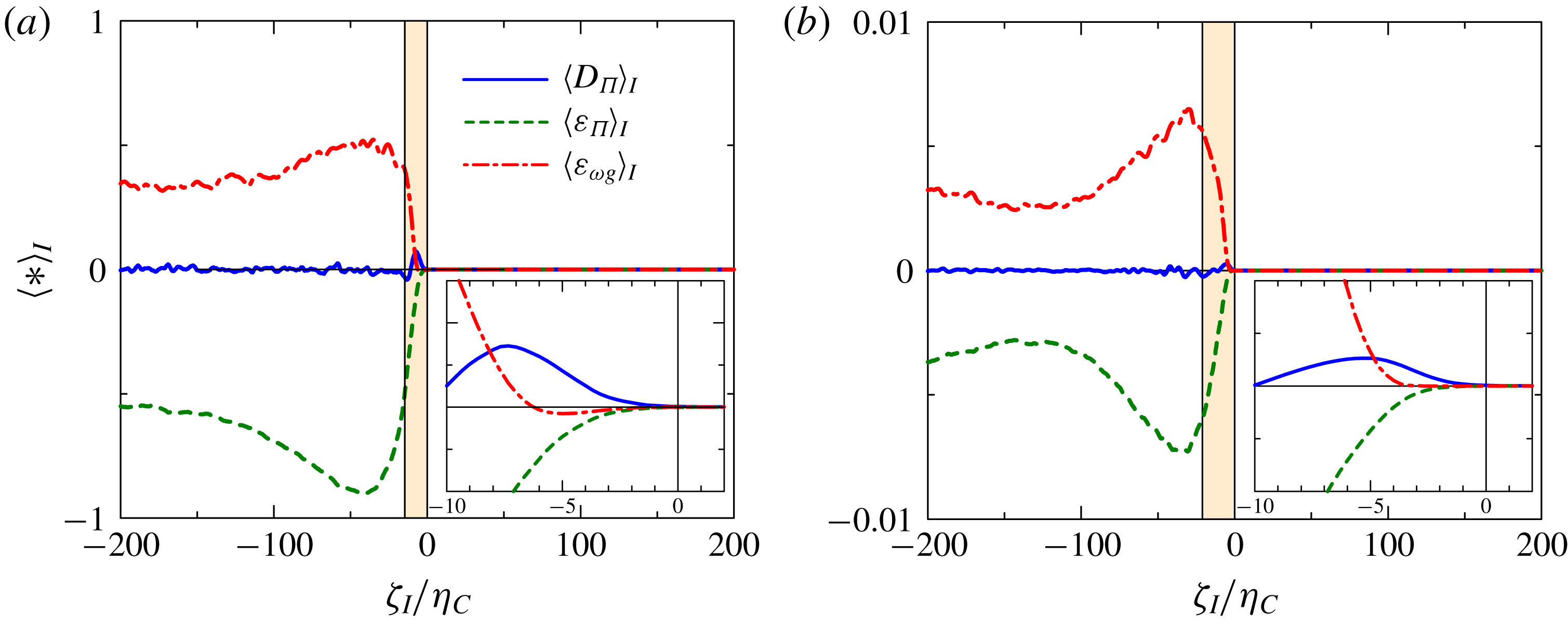
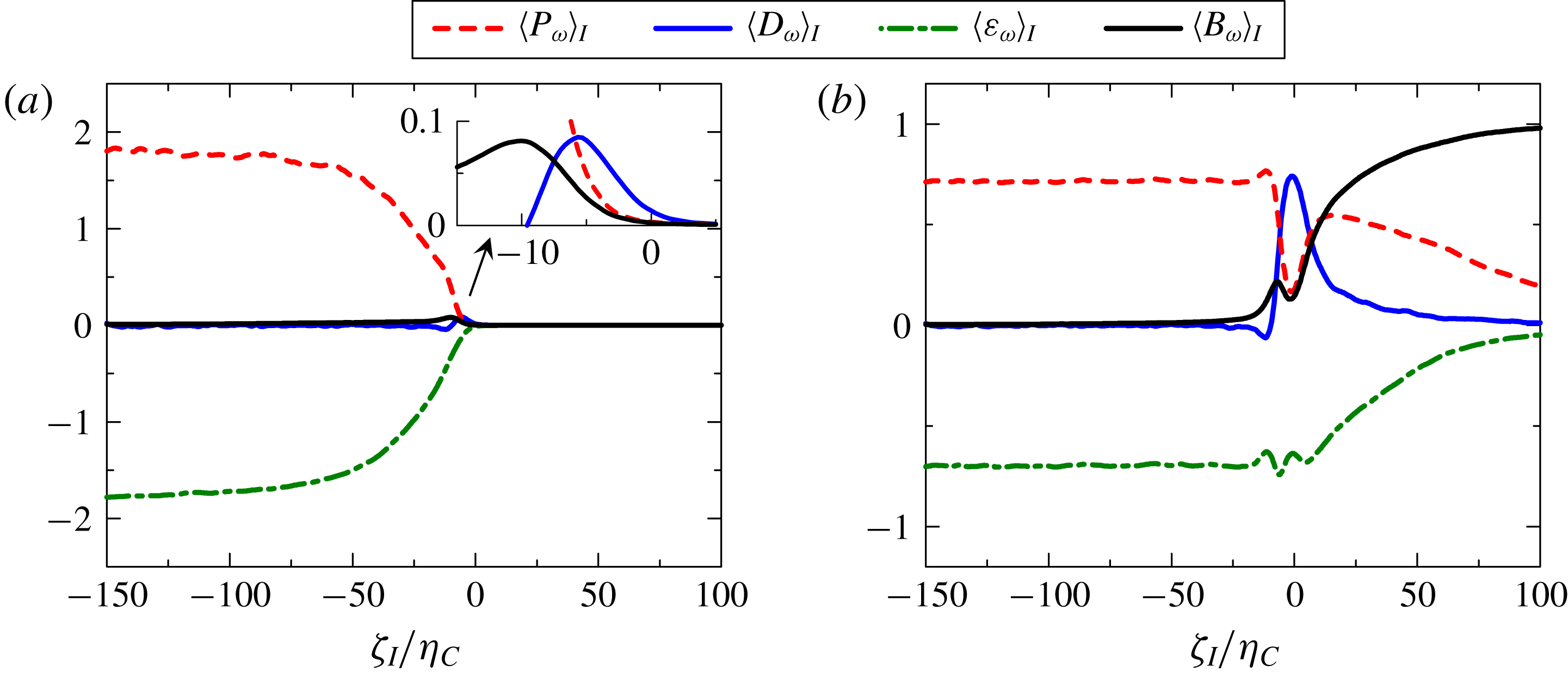
For unity Prandtl number, as in the present DNS, we can derive a somewhat simplified form for the governing equation for the potential enstrophy as (Watanabe et al. Reference Watanabe, Riley, de Bruyn Kops, Diamessis and Zhou2016a )

(3.4) $$\begin{eqnarray}\displaystyle & \displaystyle {\displaystyle \frac{\text{D}(\unicode[STIX]{x1D6F1}^{2}/2)}{\text{D}t}}={\displaystyle \frac{1}{Re}}{\displaystyle \frac{\unicode[STIX]{x2202}^{2}\unicode[STIX]{x1D6F1}^{2}/2}{\unicode[STIX]{x2202}x_{j}\unicode[STIX]{x2202}x_{j}}}-{\displaystyle \frac{1}{Re}}{\displaystyle \frac{\unicode[STIX]{x2202}\unicode[STIX]{x1D6F1}}{\unicode[STIX]{x2202}x_{j}}}{\displaystyle \frac{\unicode[STIX]{x2202}\unicode[STIX]{x1D6F1}}{\unicode[STIX]{x2202}x_{j}}}-{\displaystyle \frac{2}{Re}}\unicode[STIX]{x1D6F1}{\displaystyle \frac{\unicode[STIX]{x2202}\unicode[STIX]{x1D714}_{i}}{\unicode[STIX]{x2202}x_{j}}}{\displaystyle \frac{\unicode[STIX]{x2202}G_{i}}{\unicode[STIX]{x2202}x_{j}}}, & \displaystyle\end{eqnarray}$$

where $G_{i}=\unicode[STIX]{x2202}\unicode[STIX]{x1D70C}/\unicode[STIX]{x2202}x_{i}$ is the total density gradient. The first, second and last terms on the right-hand side are the diffusion ( $D_{\unicode[STIX]{x1D6F1}}$ ), the dissipation ( $\unicode[STIX]{x1D700}_{\unicode[STIX]{x1D6F1}}$ ) and the mixed production–dissipation ( $\unicode[STIX]{x1D700}_{\unicode[STIX]{x1D714}G}$ ) terms, respectively. It should be noted that all of these terms are caused by the molecular/viscous effects while enstrophy is also influenced by inviscid vortex stretching/compression. The conditional average of each term is shown in figure 12 at $t=80$ and $t=160$ for R6F10. We find that $\unicode[STIX]{x1D700}_{\unicode[STIX]{x1D714}G}$ amplifies while $\unicode[STIX]{x1D700}_{\unicode[STIX]{x1D6F1}}$ dissipates the potential enstrophy on average in the turbulent region. As the turbulence edge ( $\unicode[STIX]{x1D701}_{I}=0$ ) is approached from the turbulent region, $\langle \unicode[STIX]{x1D700}_{\unicode[STIX]{x1D714}G}\rangle _{I}$ decreases to 0 and the diffusion term $D_{\unicode[STIX]{x1D6F1}}$ becomes the dominant term in the growth of the potential enstrophy, as the turbulent region grows by diffusion. This relation between $\unicode[STIX]{x1D700}_{\unicode[STIX]{x1D714}G}$ and $D_{\unicode[STIX]{x1D6F1}}$ is very similar to the one between the inviscid vortex stretching term $\unicode[STIX]{x1D714}_{i}\unicode[STIX]{x1D61A}_{ij}\unicode[STIX]{x1D714}_{i}$ and viscous diffusion term $(1/Re)\unicode[STIX]{x1D6FB}^{2}(\unicode[STIX]{x1D714}_{i}\unicode[STIX]{x1D714}_{i}/2)$ in the enstrophy equation near the TNTI layer in non-stratified turbulent flows (Jahanbakhshi, Vaghefi & Madnia Reference Jahanbakhshi, Vaghefi and Madnia2015; Watanabe et al. Reference Watanabe, Sakai, Nagata, Ito and Hayase2015). It was also found in stratified wakes that $\unicode[STIX]{x1D700}_{\unicode[STIX]{x1D714}G}$ amplifies $\unicode[STIX]{x1D6F1}^{2}/2$ for the fluid with large $\unicode[STIX]{x1D6F1}^{2}/2$ , while fluids with small $\unicode[STIX]{x1D6F1}^{2}/2$ gain potential vorticity through the diffusion term $D_{\unicode[STIX]{x1D6F1}}$ (Watanabe et al. Reference Watanabe, Riley, de Bruyn Kops, Diamessis and Zhou2016a ). The conditional profiles in figure 12 agree with these results in stratified wakes: $\unicode[STIX]{x1D700}_{\unicode[STIX]{x1D714}G}$ increases $\unicode[STIX]{x1D6F1}^{2}/2$ in the turbulent core region with large $\langle \unicode[STIX]{x1D6F1}^{2}/2\rangle _{I}$ ; and the diffusion term $D_{\unicode[STIX]{x1D6F1}}$ increases $\unicode[STIX]{x1D6F1}^{2}/2$ near the turbulence edge, where $\langle \unicode[STIX]{x1D6F1}^{2}/2\rangle _{I}$ is small.

Figure 12.

Conditional budget of potential enstrophy for run R6F10 at (a)  $t=80$ and (b) $t=160$ . The insets show the potential enstrophy budget very close to the turbulence edge. The TNTI layer defined in figure 11 is highlighted.

Figure 13.

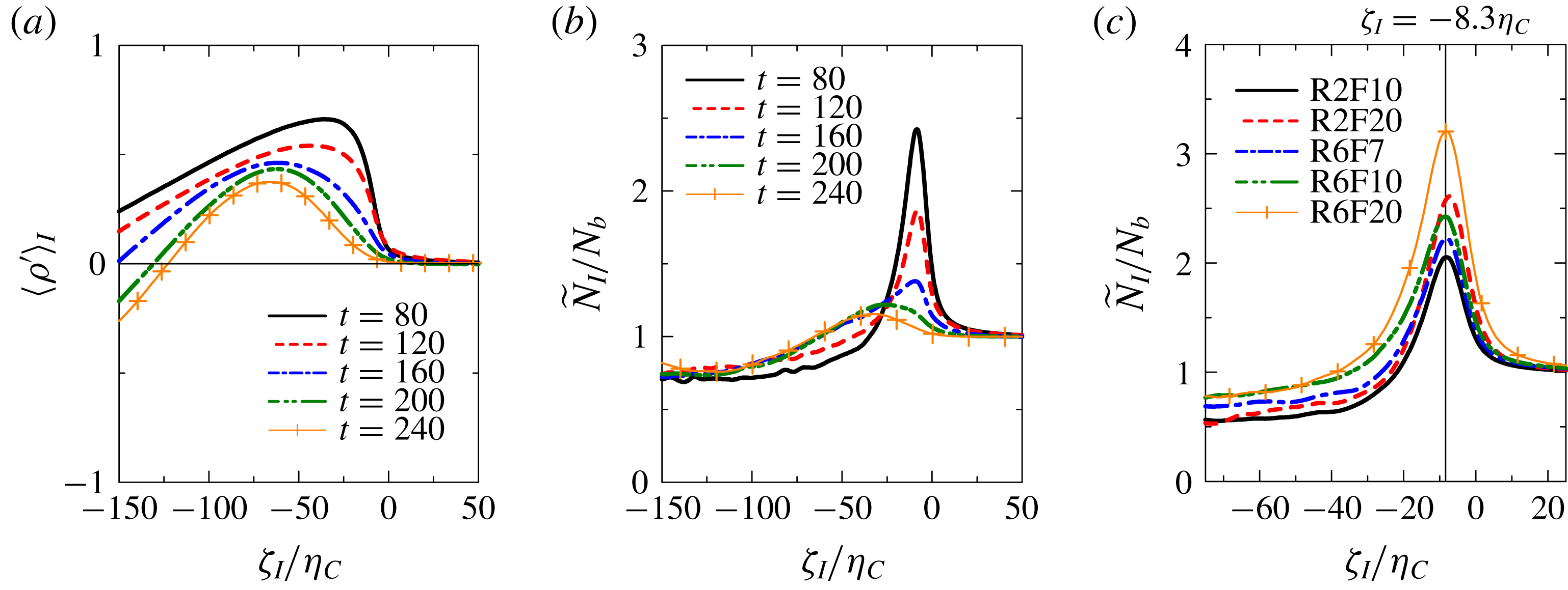
Temporal evolutions of (a) the mean value of density perturbation from a linearly varying part and (b) buoyancy frequency near the TNTI layer in R6F10. (c) Comparisons of buoyancy frequency near the TNTI layer at $t=80$ among all of the DNS dataset.

Figure 14.

Isopycnals near the TNTI layer on an $x$ – $z$ plane at (a)  $t=120$ and (b) $t=200$ in R6F10. Intervals of the isopycnals are $0.2$ . Colour contour indicates potential enstrophy.

3.4 Turbulence characteristics near the TNTI layer

Conditional statistics related to the density field are presented in figure 13. The conditional average of $\unicode[STIX]{x1D70C}^{\prime }$ , $\langle \unicode[STIX]{x1D70C}^{\prime }\rangle _{I}$ , is shown in figure 13(a). It should be noted that the results are presented for the upper interface. Positive $\langle \unicode[STIX]{x1D70C}^{\prime }\rangle _{I}$ near the TNTI layer confirms that heavier fluid is vertically transported towards the upper TNTI layer. The $\langle \unicode[STIX]{x1D70C}^{\prime }\rangle _{I}$ value rapidly decreases towards 0 as the turbulence edge is approached. Thus, there is almost no transfer of heavier fluid across the upper TNTI layer into the non-turbulent region. Figure 13(b) shows the temporal evolution of the buoyancy frequency ${\tilde{N}}_{I}/N_{b}$ near the TNTI layer in R6F10, where ${\tilde{N}}_{I}=\sqrt{-(g/\unicode[STIX]{x1D70C}_{0})\langle \unicode[STIX]{x2202}\tilde{\unicode[STIX]{x1D70C}}/\unicode[STIX]{x2202}\tilde{z}\rangle _{I}}$ . Owing to the vertical transport of $\unicode[STIX]{x1D70C}^{\prime }$ towards the TNTI layer, the buoyancy effects are locally strengthened in time near the TNTI layer, as found from a large peak of ${\tilde{N}}_{I}/N_{b}$ . Near the TNTI layer, ${\tilde{N}}_{I}/N_{b}$ is much larger than in the turbulent core region, implying that the buoyancy forces become stronger near the TNTI layer. It is also found that the location of peaks of ${\tilde{N}}_{I}/N_{b}$ shifts towards the turbulent core region with time. This tendency is closely related to the temporal evolution of the TNTI layer thickness. Figure 13(c) compares ${\tilde{N}}_{I}/N_{b}$ at $t=80$ for all cases. The plot of ${\tilde{N}}_{I}/N_{b}$ has a peak at $\unicode[STIX]{x1D701}_{I}=-8.3\unicode[STIX]{x1D702}_{C}$ while the TNTI thickness is approximately $13\unicode[STIX]{x1D702}_{C}$ at this time. Thus, the buoyancy frequency reaches the maximum within the TNTI layer.

In figure 14, the isopycnals near the TNTI layer are visualized with colour contours of potential enstrophy at $t=120$ and $200$ . The buoyancy Reynolds number on the centreline $Re_{b}$ (figure 5) is large enough for small-scale turbulence to exist in the turbulent region at $t=120$ , while $Re_{b}$ is below 10 at $t=200$ . Figure 14(a) shows that the overturning motions due to small-scale turbulence exist in the turbulent region with high potential vorticity, while they are absent in the non-turbulent fluid. It is also found that the density gradient tends to be large near the TNTI layer at $t=120$ . The overturning motions appear in only a small part of the turbulent region at $t=200$ , as seen in figure 14(b). The isopycnals are mostly flat near the TNTI layer and the overturning motions occur in the turbulent region far from the turbulence edge.

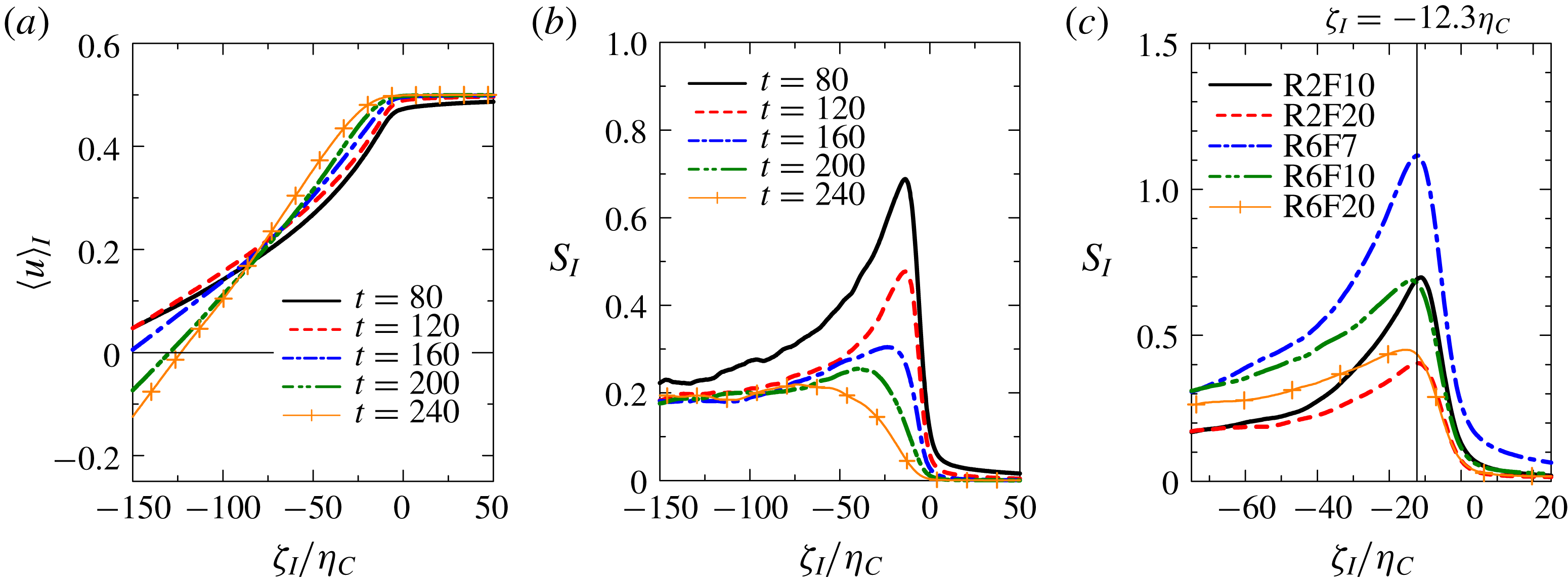
Figure 15(a) shows the conditional mean streamwise velocity $\langle u\rangle _{I}$ for R6F10. Similarly to other quantities discussed above, $\langle u\rangle _{I}$ changes slope near the TNTI layer. Its slope increases as the TNTI layer is approached from the turbulent core region. The change in slope in $\langle u\rangle _{I}$ across the TNTI layer is not, however, as significant as for the other quantities. It is also found that the location of $\unicode[STIX]{x1D701}_{I}$ where $\langle u\rangle _{I}$ starts to deviate from the non-turbulent value moves with time further inside of the turbulent region. The mean shear related to the streamwise velocity near the TNTI layer can be defined as $S_{I}=\langle \unicode[STIX]{x2202}u/\unicode[STIX]{x2202}z\rangle _{I}$ . Figure 15(b) shows $S_{I}$ at the same times as in figure 15(a). Strong mean shear appears near the TNTI layer at early times, while the shear is weakened with time as found from the peak in $S_{I}$ decreasing. At later times $S_{I}$ decreases from the turbulent to the non-turbulent region without a significant peak, although the buoyancy frequency $N_{I}$ has a peak near the TNTI. Figure 15(c) compares $S_{I}$ at $t=80$ for all cases of the DNS. Peaks in $S_{I}$ appear at $\unicode[STIX]{x1D701}_{I}=-12.3\unicode[STIX]{x1D702}_{C}$ , which is different from the peak for the buoyancy frequency in figure 13(c). Comparison between $S_{I}$ and $N_{I}$ in figures 13(c) and 15(c) shows that the flow near the outer edge of the TNTI layer is dominated more by the buoyancy than by the shearing motion due to the mean horizontal flow.

Figure 15.

(a) Conditional average of the streamwise mean velocity. (b) Vertical mean shear, $S_{I}=\langle \unicode[STIX]{x2202}u/\unicode[STIX]{x2202}z\rangle _{I}$ , near the TNTI layer. (c) Comparisons of $S_{I}$ at $t=80$ among all of the DNS dataset.

Figure 16.

Ozmidov scale $L_{OI}$ and Kolmogorov scale $\unicode[STIX]{x1D702}_{I}$ near the TNTI layer in R6F10.

Figure 17.

(a) Richardson number $Ri_{gI}=N_{I}^{2}/S_{I}^{2}$ , (b) buoyancy Reynolds number 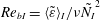$Re_{bI}=\langle \tilde{\unicode[STIX]{x1D700}}\rangle _{I}/\unicode[STIX]{x1D708}\tilde{N_{I}}^{2}$ and (c) turbulent Froude number $Fr_{I}=\langle \tilde{\unicode[STIX]{x1D700}}\rangle _{I}/\tilde{N_{I}}\tilde{u} _{rmsI}^{2}$ near the TNTI layer (R6F10).

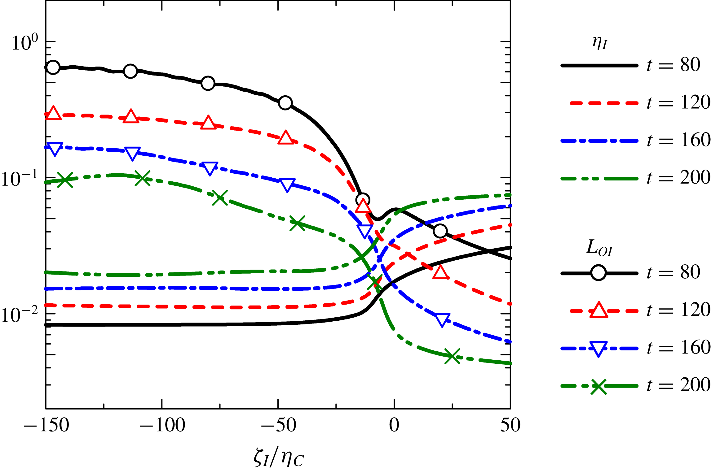
The Ozmidov scale and the Kolmogorov scale near the TNTI layer can be defined as $\tilde{L}_{OI}=(\langle \tilde{\unicode[STIX]{x1D700}}\rangle _{I}/{\tilde{N}}_{I}^{3})^{1/2}$ and $\tilde{\unicode[STIX]{x1D702}}_{I}=(\unicode[STIX]{x1D708}^{3}/\langle \tilde{\unicode[STIX]{x1D700}}\rangle _{I})^{1/4}$ , respectively. The Ozmidov scale indicates the size of the largest eddy that is unaffected by buoyancy. The kinetic energy dissipation rate appears in the definition of the Ozmidov scale as the measure of strength of turbulence. Therefore, the Ozmidov scale near the TNTI layer is also given as a function of $\unicode[STIX]{x1D701}_{I}$ because $\langle \unicode[STIX]{x1D700}\rangle _{I}$ changes sharply across the TNTI layer. Figure 17(a) shows the temporal evolution of $L_{OI}$ and $\unicode[STIX]{x1D702}_{I}$ for R6F10. The value of $\unicode[STIX]{x1D702}_{I}$ increases from the turbulent region towards the non-turbulent region because the Kolmogorov scale increases as the turbulence decays. In contrast, $L_{OI}$ decreases sharply from the turbulent towards the non-turbulent region because of small $\langle \unicode[STIX]{x1D700}\rangle _{I}$ and large $N_{I}$ (figure 13 b) within the TNTI layer.

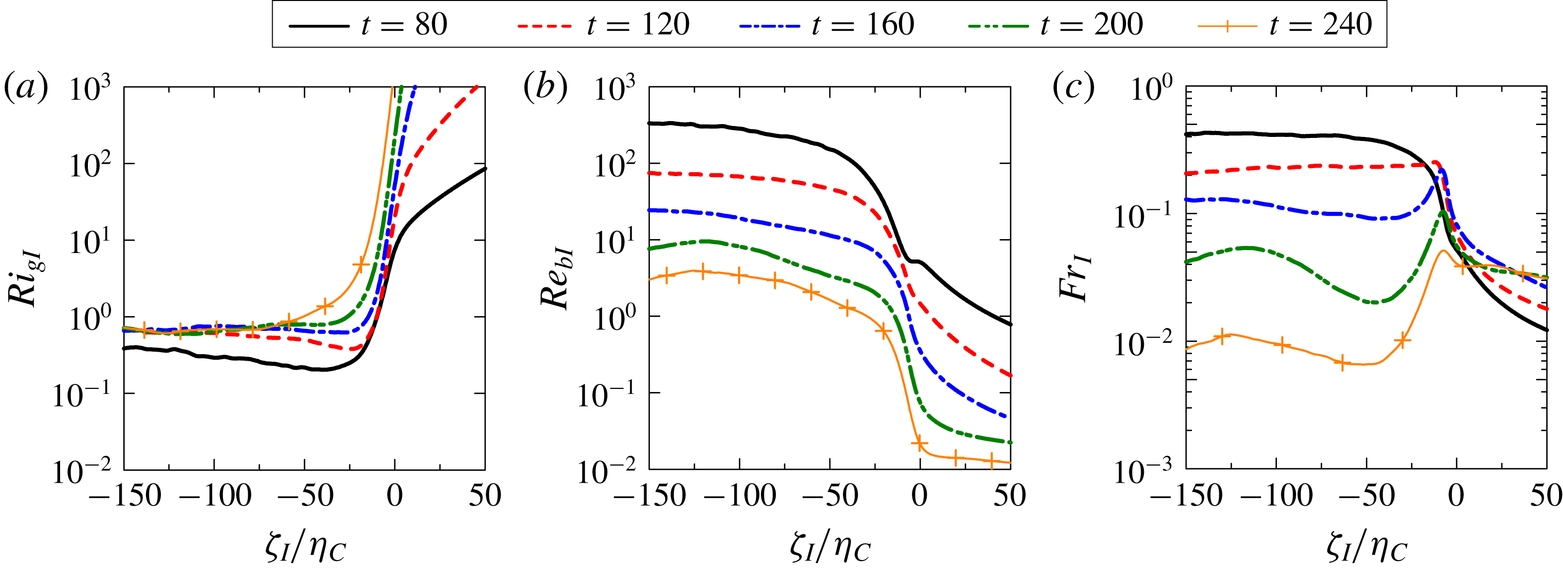
Near the turbulence edge the gradient Richardson number can be defined as $Ri_{gI}=N_{I}^{2}/S_{I}^{2}$ . Figure 17(a) shows the temporal evolution of $Ri_{gI}$ for R6F10. As expected from $N_{I}$ and $S_{I}$ , $Ri_{gI}$ drastically increases across the TNTI layer towards the non-turbulent region. A very large value of $Ri_{gI}$ starts to appear in the turbulent region near the TNTI layer for later times (i.e.  $\unicode[STIX]{x1D701}_{I}/\unicode[STIX]{x1D702}_{C}\approx -40$ at $t=240$ ), although $Ri_{gI}$ hardly changes with time from $t=120$ to $240$ in the turbulent region far from the turbulence edge ( $\unicode[STIX]{x1D701}_{I}\approx -150\unicode[STIX]{x1D702}_{C}$ ).

Similarly to $Ri_{gI}$ , we can also define the buoyancy Reynolds number $Re_{bI}$ near the TNTI layer with the conditional average as

(3.5) $$\begin{eqnarray}\displaystyle & \displaystyle Re_{bI}=\left({\displaystyle \frac{\tilde{L}_{OI}}{\tilde{\unicode[STIX]{x1D702}}_{I}}}\right)^{4/3}={\displaystyle \frac{\langle \tilde{\unicode[STIX]{x1D700}}\rangle _{I}}{\unicode[STIX]{x1D708}{\tilde{N}}_{I}^{2}}}. & \displaystyle\end{eqnarray}$$

Figure 17(b) shows a plot of $Re_{bI}$ for run R6F10. It can be seen that $Re_{bI}$ decreases gradually from the turbulent core region to the TNTI layer, and rapidly decreases across the TNTI layer, consistent with its behaviour for stably stratified wakes (Watanabe et al. Reference Watanabe, Riley, de Bruyn Kops, Diamessis and Zhou2016a ). Since $Re_{bI}$ also decreases with time, the turbulent region near the TNTI layer reaches the low buoyancy-Reynolds-number regime $Re_{bI}\leqslant O(10^{0})$ , even though $Re_{bI}$ is large enough for the small-scale turbulence to exist in the turbulent core region far from the TNTI layer. This small value of $Re_{bI}$ near the turbulence edge is consistent with the visualization of isopycnals in figure 14(b), where the overturning motion can be found in the turbulent region far from the turbulence edge but not near the turbulence edge. This indicates that the value of the buoyancy Reynolds number near the TNTI layer plays an important role in the flow dynamics of turbulence near the TNTI layer in a stably stratified fluid.

Figure 17(c) shows the turbulent Froude number $Fr_{I}=\langle \tilde{\unicode[STIX]{x1D700}}\rangle _{I}/{\tilde{N}}_{I}\tilde{u} _{rmsI}^{2}$ near the TNTI layer for R6F10; $Fr_{I}$ can be related to the ratio of buoyancy time scale to the time scale of horizontal turbulence motions. In the turbulent core region, $Fr_{I}$ decays with time as the buoyancy dominates the flow in the later time.

Figure 18.

Buoyancy Reynolds number $Re_{bI}(\unicode[STIX]{x1D701}_{I})$ at (a) $\unicode[STIX]{x1D701}_{I}/\unicode[STIX]{x1D702}_{C}=-35$ and (b)  $\unicode[STIX]{x1D701}_{I}/\unicode[STIX]{x1D702}_{C}=-50$ plotted against $Re_{bI}$ at $\unicode[STIX]{x1D701}_{I}/\unicode[STIX]{x1D702}_{C}=-40$ . Solid line represents $Re_{bI}(-35\unicode[STIX]{x1D702}_{C})=0.9Re_{bI}(-40\unicode[STIX]{x1D702}_{C})$ in (a) and $Re_{bI}(-50\unicode[STIX]{x1D702}_{C})=1.2Re_{bI}(-40\unicode[STIX]{x1D702}_{C})$ in (b).

3.5 Dependences on the buoyancy Reynolds number near the TNTI layer

We consider the dependence of the TNTI layer characteristics on the buoyancy Reynolds number $Re_{bI}$ . We take the turbulence characteristics from the conditional statistics at $\unicode[STIX]{x1D701}_{I}=-40\unicode[STIX]{x1D702}_{C}$ . 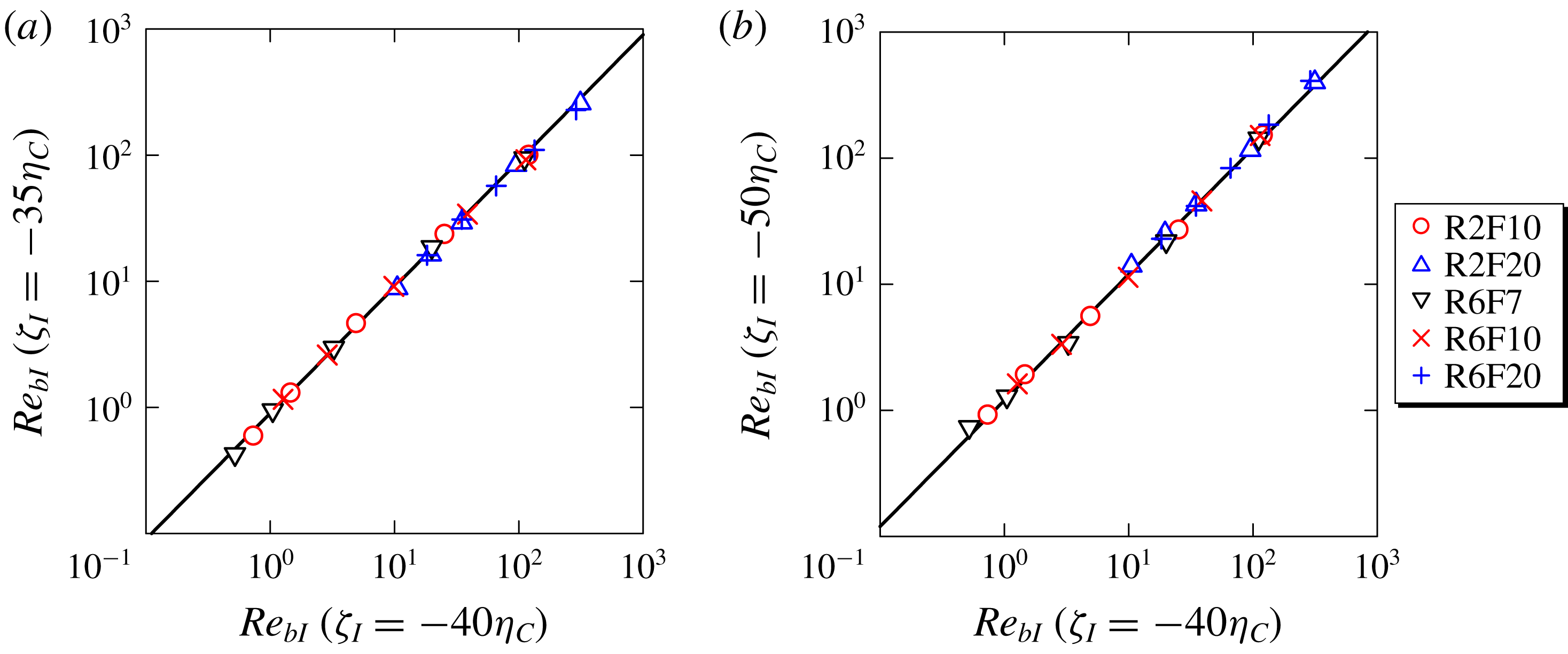Since the dependence of the conditional statistics at this location is weaker than in the region much closer to the turbulence edge $\unicode[STIX]{x1D701}_{I}\approx -5\unicode[STIX]{x1D702}_{C}$ , the results presented here are qualitatively insensitive to small changes of the location where the turbulence characteristics are taken. We can confirm this from figure 18, where $Re_{bI}(\unicode[STIX]{x1D701}_{I})$ at $\unicode[STIX]{x1D701}_{I}/\unicode[STIX]{x1D702}_{C}=-35$ or $\unicode[STIX]{x1D701}_{I}/\unicode[STIX]{x1D702}_{C}=-50$ is plotted against $Re_{bI}$ at $\unicode[STIX]{x1D701}_{I}/\unicode[STIX]{x1D702}_{C}=-40$ . A solid line denotes $Re_{bI}(-35\unicode[STIX]{x1D702}_{C})=0.9Re_{bI}(-40\unicode[STIX]{x1D702}_{C})$ and $Re_{bI}(-50\unicode[STIX]{x1D702}_{C})=1.2Re_{bI}(-40\unicode[STIX]{x1D702}_{C})$ , and $Re_{bI}$ at $\unicode[STIX]{x1D701}_{I}/\unicode[STIX]{x1D702}_{C}=-35$ and $-50$ is almost proportional to the value at $\unicode[STIX]{x1D701}_{I}/\unicode[STIX]{x1D702}_{C}=-40$ . Even if the turbulence characteristics are taken from a location slightly different from $\unicode[STIX]{x1D701}_{I}/\unicode[STIX]{x1D702}_{C}=-40$ , the influences result only in a small shift along a $Re_{bI}$ axis in the following plots.

Figure 19.

Thickness of the TNTI layer, $\unicode[STIX]{x1D6FF}_{I}$ , plotted against buoyancy Reynolds number $Re_{bI}$ . Here $\unicode[STIX]{x1D6FF}_{I}$ is normalized by Kolmogorov scale $\unicode[STIX]{x1D702}_{I}=(\unicode[STIX]{x1D708}^{3}/\langle \unicode[STIX]{x1D700}\rangle _{I})^{1/4}$ in (a) and by vertical viscous scale $l_{vI}=l_{hI}Re^{-1/2}$ in (b), where $l_{hI}=u_{rmsI}^{3}/\langle \unicode[STIX]{x1D700}\rangle _{I}$ is the horizontal length scale. The turbulence characteristics used for the normalization are taken near the TNTI layer at $\unicode[STIX]{x1D701}_{I}/\unicode[STIX]{x1D702}_{C}=-40$ .

The TNTI layer in non-stratified flows forms around the vortical structures near the outer edge of the turbulent region, where high vorticity is concentrated in small-scale tube-like structures (da Silva, Dos Reis & Pereira Reference da Silva, Dos Reis and Pereira2011). Therefore, it is natural to relate the length scale of the small-scale vortical structures to the thickness of the TNTI layer, where the vorticity level between the non-turbulent and turbulent regions is adjusted over the distance related to the length scale of the structures (Watanabe et al. Reference Watanabe, Jaulino, Taveira, da Silva, Nagata and Sakai2017a ). 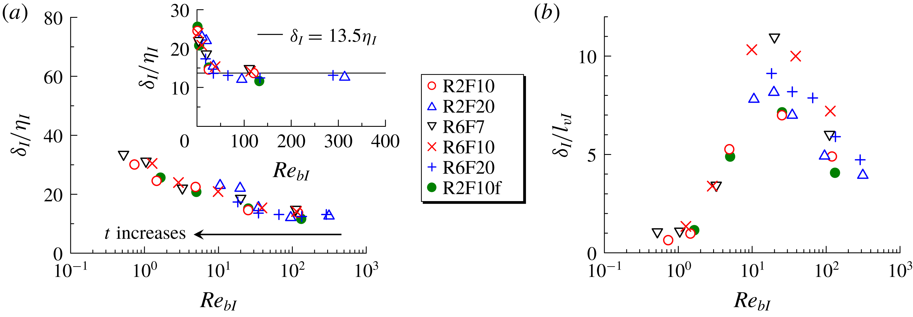Previous studies have reported that the radius of intense vortical structures scales with the Kolmogorov scale (Jimenez & Wray Reference Jimenez and Wray1998; Tanahashi, Iwase & Miyauchi Reference Tanahashi, Iwase and Miyauchi2001). Therefore, we expect that the TNTI layer thickness scales with the Kolmogorov scale in stably stratified shear layers at high buoyancy Reynolds number, in which the small-scale vortical structures exist as in non-stratified flows. We plot the TNTI layer thickness $\unicode[STIX]{x1D6FF}_{I}$ , normalized by the Kolmogorov scale near the TNTI layer $\unicode[STIX]{x1D702}_{I}$ , as a function of the buoyancy Reynolds number $Re_{bI}$ in figure 19. The figure includes data at $t=80$ , 120, 160, 200 and 240. As expected from the above discussion, $\unicode[STIX]{x1D6FF}_{I}/\unicode[STIX]{x1D702}_{I}$ tends to a constant value for large $Re_{bI}$ , where the average of $\unicode[STIX]{x1D6FF}_{I}/\unicode[STIX]{x1D702}_{I}$ for $Re_{bI}>30$ is 13.5, which is close to the TNTI layer thickness observed in non-stratified free shear flows (Watanabe et al. Reference Watanabe, Nagata and da Silva2017b ). The $\unicode[STIX]{x1D6FF}_{I}/\unicode[STIX]{x1D702}_{I}$ value increases as $Re_{bI}$ decreases once $Re_{bI}$ reaches below 30. Because a large part of the turbulence edge faces in the vertical direction (figure 9), we can relate the TNTI layer thickness to the vertical length scale of the flow. The characteristic vertical length scale changes depending on the buoyancy Reynolds number in stably stratified flows (Godoy-Diana, Chomaz & Billant Reference Godoy-Diana, Chomaz and Billant2004). Assuming that the vertical length scale is determined by a balance between horizontal advection and vertical diffusion in stratified flows with small $Re_{b}$ (Godoy-Diana et al. Reference Godoy-Diana, Chomaz and Billant2004), we can obtain the vertical length scale as $l_{v}\sim l_{h}Re^{-1/2}$ , where $l_{v}$ and $l_{h}$ are the characteristic vertical and horizontal scales, respectively. The vertical length scale near the TNTI layer, $l_{vI}$ , can be estimated as $l_{hI}Re^{-1/2}$ , with $l_{hI}=u_{rmsI}^{3}/\langle \unicode[STIX]{x1D700}\rangle _{I}$ , where $u_{rmsI}$ is the r.m.s. streamwise velocity fluctuation computed with the conditional average. A plot of $\unicode[STIX]{x1D6FF}_{I}/l_{vI}$ against $Re_{bI}$ is shown in figure 19(b). In the plots $\unicode[STIX]{x1D6FF}_{I}/l_{vI}\approx 1$ for $Re_{bI}<2$ . Thus, the TNTI layer thickness scales with the vertical length scale in the low buoyancy-Reynolds-number regime. In the present DNS results, the data in the range of $2<Re_{bI}<30$ do not follow $\unicode[STIX]{x1D6FF}_{I}\approx 13\unicode[STIX]{x1D702}_{I}$ or $\unicode[STIX]{x1D6FF}_{I}\approx l_{vI}$ , and the TNTI layer thickness is in an intermediate regime for $2<Re_{bI}<30$ . It should be noted that the exact values that limit the intermediate regime are slightly shifted when $Re_{bI}$ is taken from different locations. However, this shift is small enough to observe the same tendency found in figure 19. The DNS with a higher spatial resolution (R2F10f) also yields the similar $Re_{bI}$ dependence in figure 19.

Figure 20.

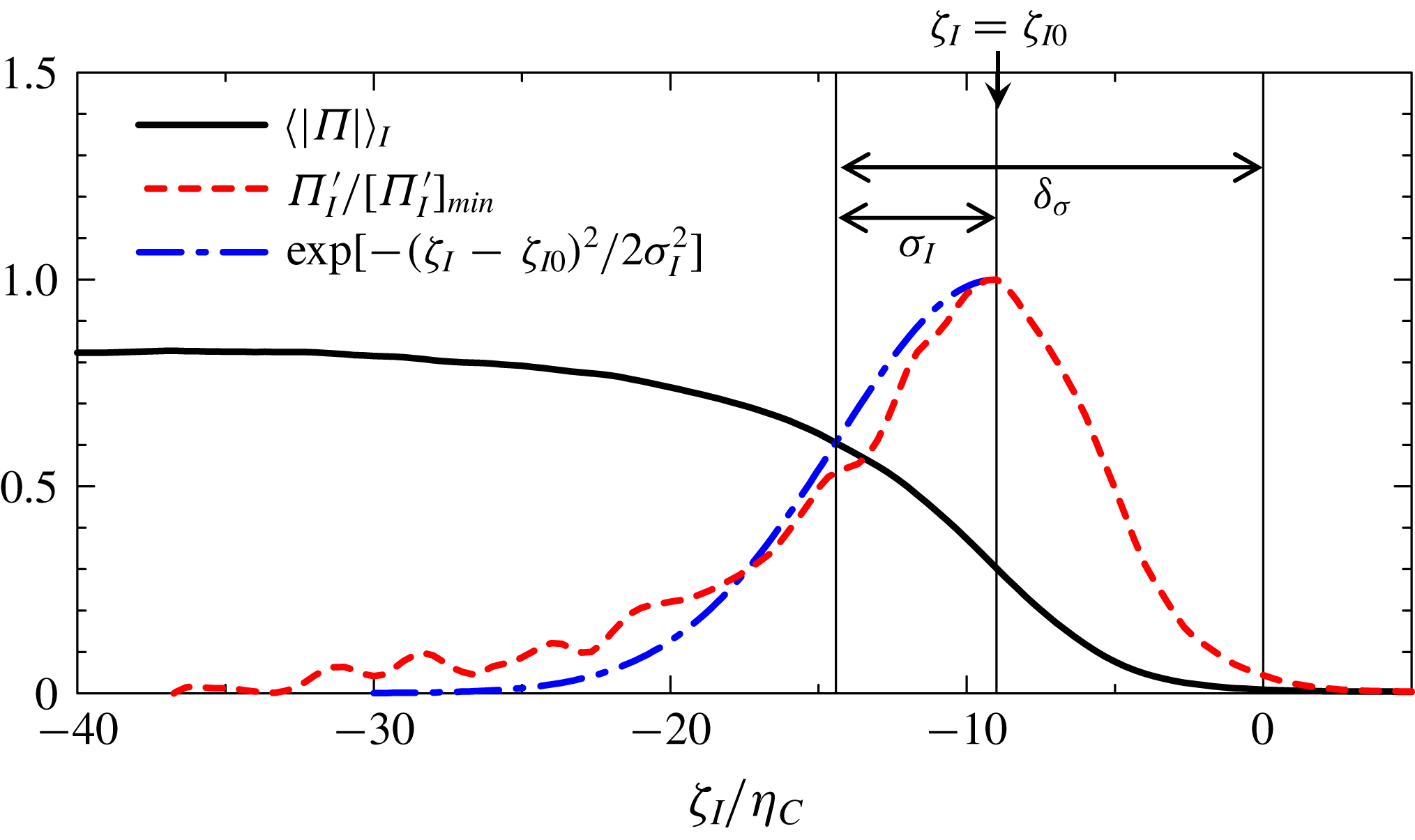
Estimation of the thickness of the TNTI layer based on a Gaussian curve fitted to $\unicode[STIX]{x1D6F1}_{I}^{\prime }=\unicode[STIX]{x2202}\langle |\unicode[STIX]{x1D6F1}|\rangle _{I}/\unicode[STIX]{x2202}\unicode[STIX]{x1D701}_{I}$ for $\unicode[STIX]{x1D701}_{I}\leqslant \unicode[STIX]{x1D701}_{I0}$ . The results are taken at $t=120$ of case R6F10.

Figure 21.

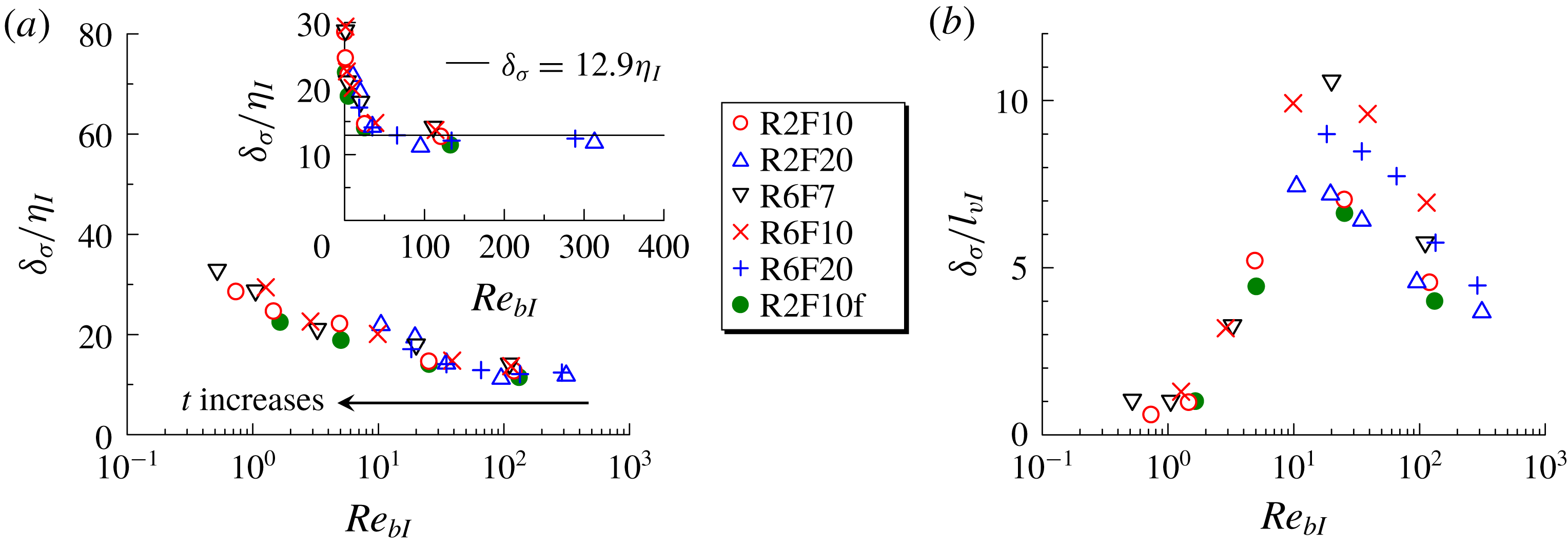
The $Re_{bI}$ dependence of the TNTI layer thickness estimated by fitting a Gaussian curve to $\unicode[STIX]{x1D6F1}_{I}^{\prime }=\unicode[STIX]{x2202}\langle |\unicode[STIX]{x1D6F1}|\rangle _{I}/\unicode[STIX]{x2202}\unicode[STIX]{x1D701}_{I}$ . The thickness estimated as $\unicode[STIX]{x1D6FF}_{\unicode[STIX]{x1D70E}}=|\unicode[STIX]{x1D701}_{I0}|+\unicode[STIX]{x1D70E}_{I}$ in figure 20 is normalized by (a) $\unicode[STIX]{x1D702}_{I}$ and (b) $l_{vI}$ as in figure 19.

We examine the sensitivity of the $Re_{bI}$ dependence of the TNTI layer thickness to the definition of the TNTI layer. Figure 20 shows $\langle |\unicode[STIX]{x1D6F1}|\rangle _{I}$ and $\unicode[STIX]{x1D6F1}_{I}^{\prime }$ , where $\unicode[STIX]{x1D6F1}_{I}^{\prime }$ is normalized by its minimum value $[\unicode[STIX]{x1D6F1}_{I}^{\prime }]_{min}$ that appears within the TNTI layer. We denote the location at which $\unicode[STIX]{x1D6F1}_{I}^{\prime }/[\unicode[STIX]{x1D6F1}_{I}^{\prime }]_{min}=1$ by $\unicode[STIX]{x1D701}_{I0}$ . Here, the thickness of the TNTI layer is estimated by approximating $\unicode[STIX]{x1D6F1}_{I}^{\prime }/[\unicode[STIX]{x1D6F1}_{I}^{\prime }]_{min}$ by a Gaussian curve. A nonlinear least-squares method applied for $\unicode[STIX]{x1D701}_{I}<\unicode[STIX]{x1D701}_{I0}$ gives $\text{exp}[-(\unicode[STIX]{x1D701}_{I}-\unicode[STIX]{x1D701}_{I0})^{2}/2\unicode[STIX]{x1D70E}_{I}]$ as shown in figure 20. The TNTI layer thickness is given by $\unicode[STIX]{x1D6FF}_{\unicode[STIX]{x1D70E}}=|\unicode[STIX]{x1D701}_{I0}|+\unicode[STIX]{x1D70E}_{I}$ . Similarly to figure 19, $\unicode[STIX]{x1D6FF}_{\unicode[STIX]{x1D70E}}$ is plotted against $Re_{bI}$ in figure 21. The same dependence of the TNTI thickness on $Re_{bI}$ is observed for $\unicode[STIX]{x1D6FF}_{\unicode[STIX]{x1D70E}}$ .

Figure 22.

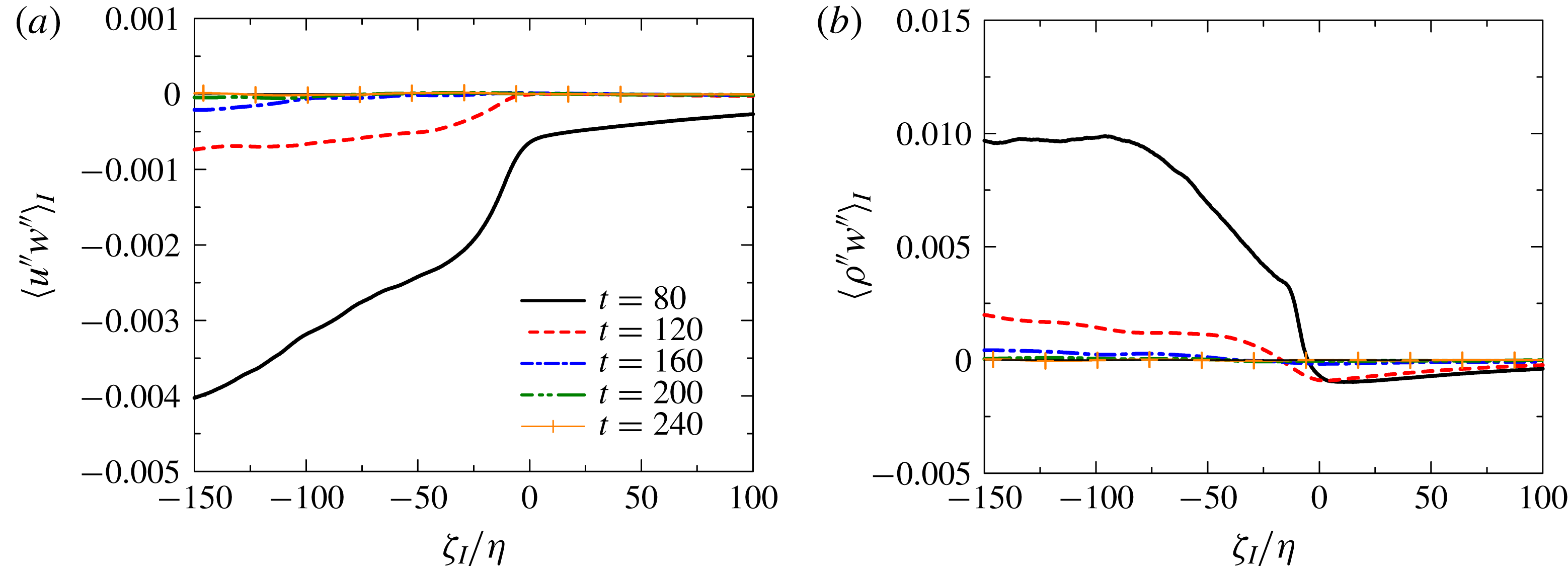
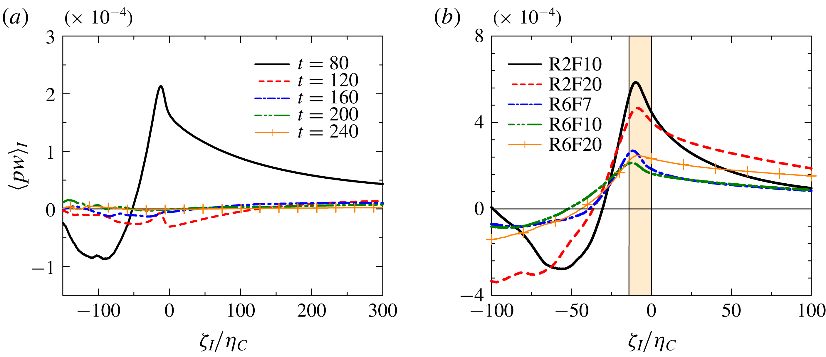
Vertical turbulent fluxes of (a) streamwise velocity $\langle u^{\prime \prime }w^{\prime \prime }\rangle _{I}$ and (b) density $\langle \unicode[STIX]{x1D70C}^{\prime \prime }w^{\prime \prime }\rangle _{I}$ near the TNTI layer. Here $u^{\prime \prime }=u-\langle u\rangle _{I}$ , $w^{\prime \prime }=w-\langle w\rangle _{I}$ and $\unicode[STIX]{x1D70C}^{\prime \prime }=\unicode[STIX]{x1D70C}^{\prime }-\langle \unicode[STIX]{x1D70C}^{\prime }\rangle _{I}$ denote the fluctuations from the conditional average.

The density and horizontal momentum are diffused by conductive (molecular) and viscous effects near the TNTI layer due to the differences in their mean values between the turbulent and non-turbulent regions. The thin TNTI layer can be maintained by density and momentum transports from the turbulent core region towards the TNTI layer (Hunt, Moustaoui & Mahalov Reference Hunt, Moustaoui and Mahalov2015). The vertical fluxes of horizontal momentum and density by turbulent velocity fluctuation are represented by $\langle u^{\prime \prime }w^{\prime \prime }\rangle _{I}$ and $\langle \unicode[STIX]{x1D70C}^{\prime \prime }w^{\prime \prime }\rangle _{I}$ , where $f^{\prime \prime }=f-\langle f\rangle _{I}$ denotes the fluctuation from the conditional mean value. Figure 22(a,b) show the temporal evolutions of $\langle u^{\prime \prime }w^{\prime \prime }\rangle _{I}$ and $\langle \unicode[STIX]{x1D70C}^{\prime \prime }w^{\prime \prime }\rangle _{I}$ for R6F10. Negative $\langle u^{\prime \prime }w^{\prime \prime }\rangle _{I}$ in the turbulent region confirms that negative momentum is transferred towards the upper TNTI layer from the turbulent core region at $t=80$ and 120. Similarly, heavy fluid is transferred towards the TNTI layer as confirmed by $\langle \unicode[STIX]{x1D70C}^{\prime \prime }w^{\prime \prime }\rangle _{I}>0$ in the turbulent region. On the other hand, the negative values of $\langle \unicode[STIX]{x1D70C}^{\prime \prime }w^{\prime \prime }\rangle _{I}$ in the non-turbulent region can more easily be interpreted as a net transfer of potential energy to the vertical component of kinetic energy, as can be seen by forming an energy equation from (2.4). Negative values of $\langle u^{\prime \prime }w^{\prime \prime }\rangle _{I}$ in the non-turbulent region are due to internal gravity waves, which transport the momentum outwards (Pham et al. Reference Pham, Sarkar and Brucker2009). Both density and momentum fluxes become small on approaching the TNTI layer in the turbulent region. A net gain/loss of density and momentum can be obtained by $-\unicode[STIX]{x2202}\langle u^{\prime \prime }w^{\prime \prime }\rangle _{I}/\unicode[STIX]{x2202}\unicode[STIX]{x1D701}_{I}$ and $-\unicode[STIX]{x2202}\langle \unicode[STIX]{x1D70C}^{\prime \prime }w^{\prime \prime }\rangle _{I}/\unicode[STIX]{x2202}\unicode[STIX]{x1D701}_{I}$ . Thus, the vertical turbulent fluxes increase the momentum and density jumps across the TNTI layer, sharpening the mean density and velocity profile within the TNTI layer, since $\unicode[STIX]{x2202}\langle u^{\prime \prime }w^{\prime \prime }\rangle _{I}/\unicode[STIX]{x2202}\unicode[STIX]{x1D701}_{I}>0$ and $\unicode[STIX]{x2202}\langle \unicode[STIX]{x1D70C}^{\prime \prime }w^{\prime \prime }\rangle _{I}/\unicode[STIX]{x2202}\unicode[STIX]{x1D701}_{I}<0$ near the TNTI layer. However, the sharpening effects due to the vertical turbulent flux are weakened with time.

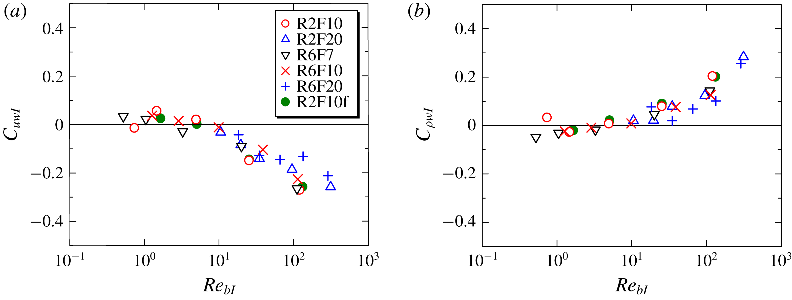
The vertical turbulent fluxes are related to the correlations of the vertical velocity with the horizontal velocity and the density. We can define the correlation coefficients as $C_{uwI}=\langle u^{\prime \prime }w^{\prime \prime }\rangle _{I}/(\langle {u^{\prime \prime }}^{2}\rangle _{I}\langle {w^{\prime \prime }}^{2}\rangle _{I})^{1/2}$ and $C_{\unicode[STIX]{x1D70C}wI}=\langle \unicode[STIX]{x1D70C}^{\prime \prime }w^{\prime \prime }\rangle _{I}/(\langle {\unicode[STIX]{x1D70C}^{\prime \prime }}^{2}\rangle _{I}\langle {w^{\prime \prime }}^{2}\rangle _{I})^{1/2}$ . Figure 23 shows $C_{uwI}$ and $C_{\unicode[STIX]{x1D70C}wI}$ plotted against the buoyancy Reynolds number $Re_{bI}$ near the TNTI layer ( $\unicode[STIX]{x1D701}_{I}=-40\unicode[STIX]{x1D702}_{C}$ ). The values of $C_{uwI}$ and $C_{\unicode[STIX]{x1D70C}wI}$ become small in magnitude as $Re_{bI}$ decreases, as the stable stratification suppresses the vertical fluxes of density and momentum. It should be noted that $C_{uwI}\approx 0$ for $Re_{bI}<10$ , for which the TNTI layer thickness normalized by the Kolmogorov scale becomes larger than the value at high buoyancy Reynolds number (see figure 11). The large mean vertical gradients of density and streamwise velocity within the TNTI layer are maintained by the vertical turbulent flux when $Re_{bI}$ is large enough for $C_{uwI}$ and $C_{\unicode[STIX]{x1D70C}wI}$ to have large values. Therefore, the temporal decay of $Re_{bI}$ is closely related to the temporal variation of the buoyancy frequency $N_{I}$ and mean shear $S_{I}$ observed in figures 13 and 15, where both $N_{I}$ and $S_{I}$ within the TNTI layer decrease with time.

Figure 23.

Correlation coefficients of (a) streamwise velocity $u$ and (b) density $\unicode[STIX]{x1D70C}^{\prime }$ with vertical velocity, defined as $C_{uwI}=\langle u^{\prime \prime }w^{\prime \prime }\rangle _{I}/\sqrt{\langle {u^{\prime \prime }}^{2}\rangle _{I}\langle {w^{\prime \prime }}^{2}\rangle _{I}}$ and $C_{\unicode[STIX]{x1D70C}wI}=\langle \unicode[STIX]{x1D70C}^{\prime \prime }w^{\prime \prime }\rangle _{I}/\sqrt{\langle {\unicode[STIX]{x1D70C}^{\prime \prime }}^{2}\rangle _{I}\langle {w^{\prime \prime }}^{2}\rangle _{I}}$ . The results near the turbulence edge ( $\unicode[STIX]{x1D701}=-40\unicode[STIX]{x1D702}_{C}$ ) are shown as a function of buoyancy Reynolds number $Re_{bI}$ at the same location.

Figure 24.

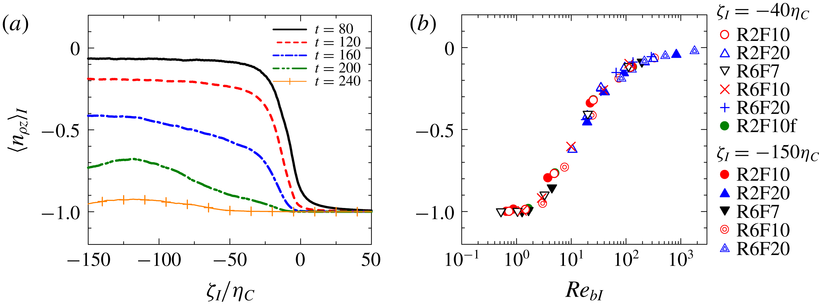
(a) Conditional average of vertical component of normalized density gradient $n_{\unicode[STIX]{x1D70C}z}=\boldsymbol{n}_{\unicode[STIX]{x1D70C}}\boldsymbol{\cdot }\boldsymbol{e}_{z}$ near the TNTI layer for R6F10. (b) Plot of $\langle n_{\unicode[STIX]{x1D70C}z}\rangle _{I}$ against buoyancy Reynolds number $Re_{bI}$ at $\unicode[STIX]{x1D701}_{I}=-40\unicode[STIX]{x1D702}_{C}$ and $-150\unicode[STIX]{x1D702}_{C}$ .

3.6 Overturning motions near the TNTI layer

Overturning motions can be identified in terms of the density gradient direction, which is represented by the normalized density gradient $\boldsymbol{n}_{\unicode[STIX]{x1D70C}}=\unicode[STIX]{x1D735}\unicode[STIX]{x1D70C}/|\unicode[STIX]{x1D735}\unicode[STIX]{x1D70C}|$ . When the isopycnals are horizontal (perpendicular to the vertical direction), the vertical component of $\boldsymbol{n}_{\unicode[STIX]{x1D70C}}$ , denoted by $n_{\unicode[STIX]{x1D70C}z}$ , is equal to $-1$ . Figure 24(a) shows the conditional average of $n_{\unicode[STIX]{x1D70C}z}$ for R6F10 for five different times. It can be seen that $\langle n_{\unicode[STIX]{x1D70C}z}\rangle _{I}$ rapidly changes across the TNTI layer. The non-turbulent fluid remains layered, similar to its state before the turbulent shear layer forms, as attested by $\langle n_{\unicode[STIX]{x1D70C}z}\rangle _{I}\approx -1$ for $\unicode[STIX]{x1D701}_{I}>0$ . Because of the overturning motions with $n_{\unicode[STIX]{x1D70C}z}>0$ in the turbulent region (also see figure 14), $\langle n_{\unicode[STIX]{x1D70C}z}\rangle _{I}$ is much larger than $-1$ for early times in this region. The $\langle n_{\unicode[STIX]{x1D70C}z}\rangle _{I}$ value decreases with time and, at very late time, $\langle n_{\unicode[STIX]{x1D70C}z}\rangle _{I}$ becomes very close to $-1$ even in the turbulent region. Thus, the overturning motions no longer occur both inside and outside of the shear layers. The decrease of $\langle n_{\unicode[STIX]{x1D70C}z}\rangle _{I}$ with time is faster for the turbulent fluid near the TNTI layer ( $\unicode[STIX]{x1D701}_{I}=-50\unicode[STIX]{x1D702}_{C}$ ) than deep inside the turbulent core region ( $\unicode[STIX]{x1D701}_{I}=-150\unicode[STIX]{x1D702}_{C}$ ). The overturning motions are absent near the TNTI layer even if they occur deep inside the turbulent core region, in agreement with the visualization in figure 14(b). Portwood et al. (Reference Portwood, de Bruyn Kops, Taylor, Salehipour and Caulfield2016) also showed that the magnitude of the density gradient is very different between the active turbulent region and the quiescent flow region. The relation between $\langle n_{\unicode[STIX]{x1D70C}z}\rangle _{I}$ and $Re_{bI}$ is examined at $\unicode[STIX]{x1D701}_{I}=-40\unicode[STIX]{x1D702}_{C}$ and $-150\unicode[STIX]{x1D702}_{C}$ in figure 24(b). The plots of all cases collapse well onto a single curve and $\langle n_{\unicode[STIX]{x1D70C}z}\rangle _{I}$ approaches to $-1$ as $Re_{bI}$ becomes small. Since $Re_{bI}$ is related to the ratio between the Ozmidov and Kolmogorov scales as in (3.6), $Re_{bI}$ can be a good measure of the existence of small-scale turbulence and overturning.

Figure 25.

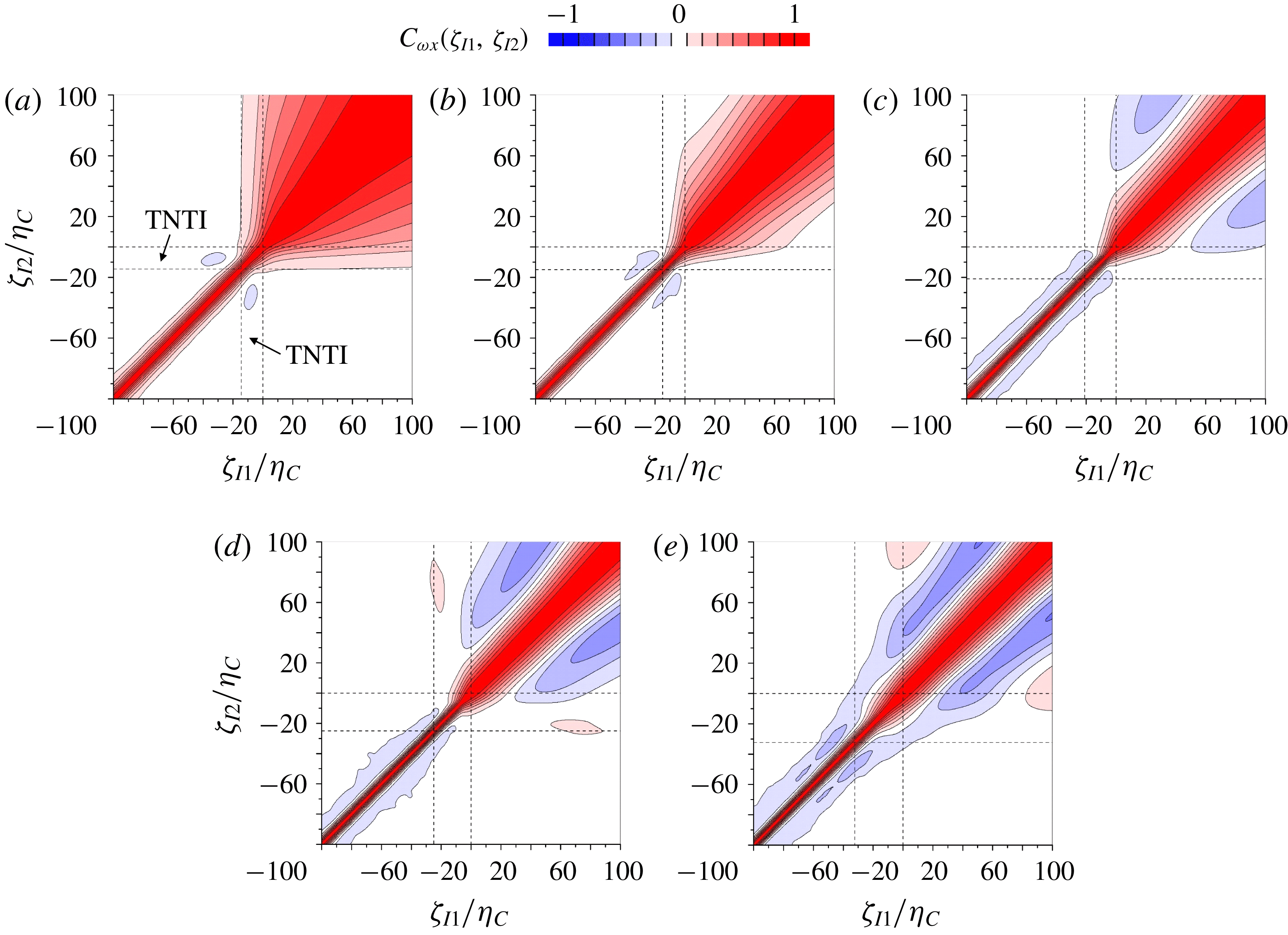
Two-point correlation of streamwise vorticity $\unicode[STIX]{x1D714}_{x}$ near the TNTI layer in R6F10 at (a) $t=80$ , (b) $t=120$ , (c) $t=160$ , (d)  $t=200$ and (e)  $t=240$ . The correlation is calculated between two points $\unicode[STIX]{x1D701}_{I}=\unicode[STIX]{x1D701}_{I1}$ and $\unicode[STIX]{x1D701}_{I}=\unicode[STIX]{x1D701}_{I2}$ based upon the interface coordinate $\unicode[STIX]{x1D701}_{I}$ . The regions between broken lines indicate the TNTI layer.

Figure 26.

(a) Conditional averages of enstrophy transport equation (3.7) at $t=80$ for R6F10. (b) The plots in (a) are normalized so that the sum of the squares of the averaged terms on the right-hand side of (3.7) is unity.

3.7 Structures of strong vorticity regions near the TNTI layer

Figure 9 confirms that the fluid outside the shear layer possesses an important level of vorticity. We investigate the structure of the vorticity field based on two-point correlations calculated between two points $\unicode[STIX]{x1D701}_{I}=\unicode[STIX]{x1D701}_{I1}$ and $\unicode[STIX]{x1D701}_{I}=\unicode[STIX]{x1D701}_{I2}$ , based upon the interface coordinate $\unicode[STIX]{x1D701}_{I}$ , as

(3.6) $$\begin{eqnarray}\displaystyle & \displaystyle C_{f}(\unicode[STIX]{x1D701}_{I1},\unicode[STIX]{x1D701}_{I2})={\displaystyle \frac{\langle f^{\prime \prime }(\unicode[STIX]{x1D701}_{I1})f^{\prime \prime }(\unicode[STIX]{x1D701}_{I2})\rangle _{I}}{\sqrt{\langle {f^{\prime \prime }}^{2}(\unicode[STIX]{x1D701}_{I1})\rangle _{I}\langle {f^{\prime \prime }}^{2}(\unicode[STIX]{x1D701}_{I2})\rangle _{I}}}}. & \displaystyle\end{eqnarray}$$

The two points are separated in the vertical direction because of the definition of $\unicode[STIX]{x1D701}_{I}$ in figure 9(a). The two-point correlations calculated for streamwise vorticity $\unicode[STIX]{x1D714}_{x}$ are shown in figure 25. The TNTI layer estimated in figure 11 is indicated by broken lines. The two-point correlation profile changes drastically with time and in space. Large positive correlation appears in a narrow region with a length of ${\sim}20\unicode[STIX]{x1D702}_{C}$ in the turbulent region. The order of this length is consistent with the characteristics length of the small-scale vortical structures, where a large vorticity is concentrated within a vortex core whose diameter is approximately $10\unicode[STIX]{x1D702}$ in non-stratified flows (Jimenez & Wray Reference Jimenez and Wray1998; Tanahashi et al. Reference Tanahashi, Iwase and Miyauchi2001; da Silva et al. Reference da Silva, Dos Reis and Pereira2011; Jahanbakhshi et al. Reference Jahanbakhshi, Vaghefi and Madnia2015). The non-turbulent fluid has a positive correlation even for two points with a large separation $|\unicode[STIX]{x1D701}_{I1}-\unicode[STIX]{x1D701}_{I2}|\gg 0$ . This is caused by the vorticity in the internal gravity waves having a much larger length scale than does the turbulence, consistent with the visualization in figure 3. Interestingly, the vorticity within the TNTI layer is positively correlated with that in the non-turbulent region, implying a relationship between the internal gravity waves and the turbulent fluid within the TNTI layer. Comparison among different time steps shows that a stronger correlation between the TNTI layer and the non-turbulent region with very large $\unicode[STIX]{x1D701}_{I}$ (non-turbulent fluid very far from the TNTI layer) can be found at earlier times.

The turbulent region at later times exhibits positive and negative values of the correlation coefficient, which is similar to the behaviour of the correlation coefficient in the internal wave region, and implies some wave behaviour. However, the vertical length scale of the structures estimated from the two-point correlation is very different between the turbulent and non-turbulent regions.

The transport equation of enstrophy $\unicode[STIX]{x1D714}_{i}\unicode[STIX]{x1D714}_{i}/2$ under the Boussinesq approximation can be written as

(3.7) $$\begin{eqnarray}\displaystyle & \displaystyle {\displaystyle \frac{\text{D}\unicode[STIX]{x1D714}_{i}\unicode[STIX]{x1D714}_{i}/2}{\text{D}t}}=\unicode[STIX]{x1D714}_{i}\unicode[STIX]{x1D61A}_{ij}\unicode[STIX]{x1D714}_{j}+{\displaystyle \frac{1}{Re}}\unicode[STIX]{x1D6FB}^{2}\unicode[STIX]{x1D714}_{i}\unicode[STIX]{x1D714}_{i}/2-{\displaystyle \frac{1}{Re}}{\displaystyle \frac{\unicode[STIX]{x2202}\unicode[STIX]{x1D714}_{i}}{\unicode[STIX]{x2202}x_{j}}}{\displaystyle \frac{\unicode[STIX]{x2202}\unicode[STIX]{x1D714}_{i}}{\unicode[STIX]{x2202}x_{j}}}+{\displaystyle \frac{4}{Fr^{2}}}\unicode[STIX]{x1D700}_{ij3}\unicode[STIX]{x1D714}_{i}{\displaystyle \frac{\unicode[STIX]{x2202}\unicode[STIX]{x1D70C}}{\unicode[STIX]{x2202}x_{j}}}. & \displaystyle\end{eqnarray}$$

In order, the terms on the right-hand side are the production term $P_{\unicode[STIX]{x1D714}}$ , viscous diffusion term $D_{\unicode[STIX]{x1D714}}$ , viscous dissipation term $\unicode[STIX]{x1D700}_{\unicode[STIX]{x1D714}}$ and baroclinic term $B_{\unicode[STIX]{x1D714}}$ . Figure 26(a) shows the conditional average of these terms at $t=80$ for R6F10. We can see the balance between the production and dissipation terms in the turbulent region as also found in other turbulent flows (e.g. Taveira & da Silva Reference Taveira and da Silva2014). The viscous diffusion has a positive value at the outer edge of the turbulence, contributing the increase of enstrophy in this region. This is consistent with the feature of the viscous superlayer that is found at the outer edge of the turbulence in non-stratified flows (van Reeuwijk & Holzner Reference van Reeuwijk and Holzner2014; Taveira & da Silva Reference Taveira and da Silva2014). It is also found that the baroclinic term $B_{\unicode[STIX]{x1D714}}$ has a positive value within the TNTI layer. The magnitude of conditional averages of (3.7) decreases towards the non-turbulent region. The relative contributions of each term are examined in figure 26(b), where the conditional averages of (3.7) are normalized so that the sum of the squares of the averaged terms on the right-hand side is unity. The same normalization is used for the turbulent kinetic energy budget in a turbulent boundary layer in order to understand the relative importance of the terms (Pope Reference Pope2000). The baroclinic term $B_{\unicode[STIX]{x1D714}}$ is a dominant term for the enstrophy increase in the non-turbulent region, where the internal gravity wave is propagating.

Figure 27.

Conditional averages of vertical outward kinetic energy flux $\langle pw\rangle _{I}$ : (a) temporal evolution in R6F10, and (b) comparison among different simulations at $t=80$ . The TNTI layer estimated in figure 11 in R6F10 is highlighted in (b).

3.8 Internal wave energy flux

The averaged vertical flux of kinetic energy due to the internal gravity waves both near the TNTI layer and outside the turbulent region is represented by the pressure–velocity correlation $\langle pw\rangle _{I}$ , whose positive value denotes the outward energy transfer. For internal waves, $\langle pw\rangle _{I}$ is often called the wave energy flux (Nash, Alford & Kunze Reference Nash, Alford and Kunze2005). A plot of $\langle pw\rangle _{I}$ for R6F10 is shown in figure 27(a). The kinetic energy at $t=80$ is transferred outwards in the region of $\unicode[STIX]{x1D701}_{I}/\unicode[STIX]{x1D702}_{C}>-50$ , although $\langle pw\rangle _{I}$ becomes close to 0 for later times. This might be related to a stronger correlation between the motion in the TNTI layer and in the non-turbulent region at earlier times, as seen in figure 25, and which indicates a greater influence of the energy flux of internal gravity waves on the TNTI layer dynamics at earlier times. We have obtained a similar time dependence of $\langle pw\rangle _{I}$ in all cases (not shown here). DNS by Pham et al. (Reference Pham, Sarkar and Brucker2009) also shows a strong time dependence of the internal wave energy flux from the stratified shear layer, which is large in early stages of the flow development, consistent with figure 27(a). Figure 27(b) compares $\langle pw\rangle _{I}$ at $t=80$ among all cases. A peak value $\langle pw\rangle _{I}$ appears near the boundary between the TNTI layer and the turbulent core region. From the averaged turbulent kinetic energy equation, it can be found that a net gain/loss of the kinetic energy due to $-\langle pw\rangle _{I}$ is given by $\mp \unicode[STIX]{x2202}\langle pw\rangle _{I}/\unicode[STIX]{x2202}\unicode[STIX]{x1D701}_{I}$ . The kinetic energy increases within the TNTI layer and in the non-turbulent region due to $\langle pw\rangle _{I}$ as depicted from $-\unicode[STIX]{x2202}\langle pw\rangle _{I}/\unicode[STIX]{x2202}\unicode[STIX]{x1D701}_{I}>0$ . In contrast, the turbulent core region near the TNTI layer loses kinetic energy by the internal wave energy flux $(-\unicode[STIX]{x2202}\langle pw\rangle _{I}/\unicode[STIX]{x2202}\unicode[STIX]{x1D701}_{I}<0)$ .

It is interesting to compare the total loss of kinetic energy due to the internal gravity wave flux with the entire kinetic energy dissipation $\unicode[STIX]{x1D700}$ that occurs in the turbulent region. We have that $\langle pw\rangle _{I}$ at $\unicode[STIX]{x1D701}_{I}=0$ is the averaged kinetic energy flux across the turbulence edge per unit horizontal area. We can define the averaged kinetic energy dissipation rate in the turbulent region per unit horizontal area as

(3.8) $$\begin{eqnarray}\displaystyle & \displaystyle \langle \tilde{\unicode[STIX]{x1D700}}\rangle _{T}={\displaystyle \frac{1}{L_{x}L_{y}}}\int _{V_{T}}\tilde{\unicode[STIX]{x1D700}}\,\text{d}\tilde{V}, & \displaystyle\end{eqnarray}$$

where $\int _{V_{T}}\text{d}\tilde{V}$ is the volume integral in the turbulent region. Table 2 summarizes $\langle pw\rangle _{I}$ and $\langle \unicode[STIX]{x1D700}\rangle _{T}$ at $t=80$ . It is found that the amount of energy extracted from the turbulent region due to the internal gravity waves is comparable to the dissipation in the turbulent region in all cases, in agreement with the DNS results of stratified wakes (Watanabe et al. Reference Watanabe, Riley, de Bruyn Kops, Diamessis and Zhou2016a ). Figure 27 shows that $\langle pw\rangle _{I}$ decreases with distance from the turbulence edge in the non-turbulent region ( $\unicode[STIX]{x1D701}_{I}$ ). The internal wave energy flux from localized turbulence is underestimated when it is evaluated in the non-turbulent region away from the turbulent region. Indeed, the internal wave energy flux evaluated on a horizontal plane away from a shear layer is smaller than the energy dissipation above the horizontal plane including the turbulent region (Pham et al. Reference Pham, Sarkar and Brucker2009).

Table 2.

Averaged vertical outward flux of kinetic energy $\langle pw\rangle _{I}$ at the turbulence edge $\unicode[STIX]{x1D701}_{I}=0$ and averaged kinetic energy dissipation rate integrated in the turbulent region $\langle \tilde{\unicode[STIX]{x1D700}}\rangle _{T}=(1/L_{x}L_{y})\int _{V_{T}}\tilde{\unicode[STIX]{x1D700}}\,\text{d}\tilde{V}$ , where $\int _{V_{T}}\text{d}\tilde{V}$ is the volume integral in the turbulent region. The results are taken at $t=80$ , at which a large energy flux across the TNTI layer is found from $\langle pw\rangle _{I}$ .