1 Introduction
On 12 December 2002, the maiden flight of the European heavy space launcher Ariane 5 ECA equipped with the new Vulcain 2 engine failed approximately three minutes after lift-off due to a deterioration of the main stage nozzle. After a complete analysis of the flight data, the inquiry board came to the conclusion that one of the aggravating factors that led to the accident was the non-exhaustive definition of the loads to which the new Vulcain 2 engine was subjected during flight (Ariane Space 2003). Subsequent investigations, including in-flight measurements of pressure fluctuations and actuator loads on the reinforced Vulcain 2 nozzle (David & Radulovic Reference David and Radulovic2005; Schwane Reference Schwane2015), confirmed that the strongest unsteady aerodynamic forces with pronounced low-frequency peaks, known as the buffet phenomenon, occur around the free stream Mach number
 $Ma_{\infty }=0.8$
and under unfavourable conditions can induce critical structural vibrations.
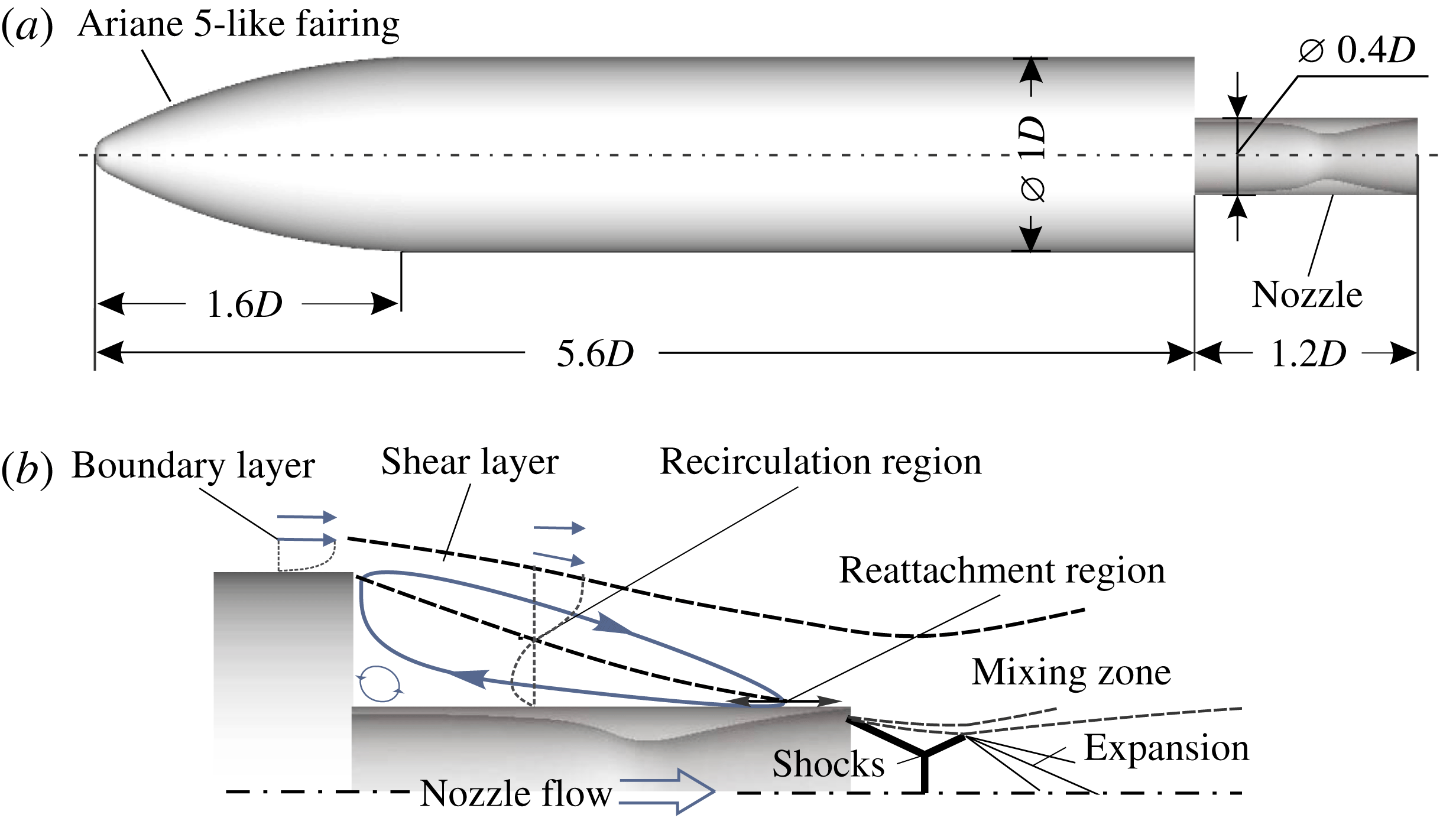
The Ariane 5 ECA accident triggered a revival of attention of the fluid mechanics community not only to the buffet phenomenon of space launchers, the first investigations of which date back to the Apollo lunar program, e.g. Coe & Nute (Reference Coe and Nute1962), Jones & Foughner (Reference Jones and Foughner1963), but also to the more general topic of the turbulent wake behind an axisymmetric backward-facing step, which had been investigated to a significantly less extent compared to its planar counterpart. Meanwhile, detailed experimental and numerical investigations on several wind tunnel and free-flight configurations ranging from simplified adjoint blunt cylinders and axisymmetric backward-facing steps up to precisely scaled models of the real European Ariane 5 launcher including solid boosters have been carried out, e.g. Deprés, Reijasse & Dussauge (Reference Deprés, Reijasse and Dussauge2004), Meliga & Reijasse (Reference Meliga and Reijasse2007), Deck & Thorigny (Reference Deck and Thorigny2007), Weiss et al. (Reference Weiss, Deck, Robinet and Sagaut2009), Hannemann et al. (Reference Hannemann, Lüdeke, Pallegoix, Ollivier, Lambare, Maseland, Geurts, Frey, Deck and Schrijer2011), Weiss & Deck (Reference Weiss and Deck2011), Schrijer et al. (Reference Schrijer, Sciacchitano, Scarano, Hanneman, Pallegoix, Maseland and Schwane2011), Pain, Weiss & Deck (Reference Pain, Weiss and Deck2014), Scharnowski et al. (Reference Scharnowski, Statnikov, Meinke, Schröder and Kähler2015), Lüdeke, Mulot & Hannemann (Reference Lüdeke, Mulot and Hannemann2015). It was demonstrated that at transonic stages of the flight trajectory, the turbulent shear layer shed from the cylindrical main body impinges on the nozzle just upstream of its end, as schematically shown in figure 1, which due to high dynamic pressure values leads to significant wall pressure fluctuations. Using classical data-based statistical analyses, i.e. both spatial and temporal, auto- and cross-correlation functions and Fourier transforms, the characteristic frequencies of the wake flow and their spatial variation could be successfully detected. However, due to the superposition of locally different periodic and stochastic phenomena, the association of every single distinct frequency with a coherent flow pattern or, more generally, a dynamic mode is not straightforward. It is often rather based on experience and best practice than on a rigorous post-processing method. In particular, the three-dimensional shape of the antisymmetric mode responsible for buffet loads is still unclear and could not be visualized yet. Therefore, to clarify the true three-dimensional shape of the wake flow modes being hidden in the multiple scales of turbulence, alternative methods capable of accurate detection and visualization of coherent flow patterns seem to be required.
(a) Geometry of the investigated generic space launcher configuration; (b) schematic of the transonic wake topology with an overexpanded nozzle jet.

Concepts appropriate for extended diagnostic purposes are the reduced-order methods such as proper orthogonal decomposition (POD) or dynamic mode decomposition (DMD). For instance, Marié et al. (Reference Marié, Druault, Lambaré and Schrijer2013) applied POD to planar particle image velocimetry (2D-PIV) and wall pressure measurements in the transonic wake of a
 $1:60$
scaled Ariane 5 wind tunnel model to identify the most energetic modes in the motion of the transonic shear layer that are responsible for dynamic loads on the nozzle. Likewise, using POD on a snapshot sequence from high-speed 2D-PIV measurements, Schrijer, Sciacchitano & Scarano (Reference Schrijer, Sciacchitano and Scarano2014) visualized the two most energetic linearly independent modes in the wake of an axisymmetric backward-facing step configuration. That is, pulsatile growth and collapse of the separated region as well as momentum exchange across the shear layer were illustrated. However, since a POD mode can generally have a multi-frequency content due to the inherent spatial, but not temporal orthogonality, it cannot be always clearly assigned to a single characteristic frequency, as it was for instance the case with the latter POD shear layer mode featuring a broadband spectrum of its time coefficients. Besides, both studies were restricted to two-dimensional longitudinal slices and the symmetry of the wind tunnel model was disturbed by an attached support such that the intrinsic three-dimensional shape of the antisymmetric mode could not be investigated.
Unlike POD, DMD (Schmid Reference Schmid2010) aims at the extraction of optimal phase-averaged structures each of which corresponds to a unique frequency and is assigned to an individual growth/decay rate. This approach can be considered as an approximation of the Koopman operator and therefore, is more suitable to analyse nonlinear systems than the conventional Fourier transforms or POD (Rowley et al. Reference Rowley, Mezic, Bagheri, Schlatter and Henningson2009; Mezić Reference Mezić2013). Being relatively new, DMD has rapidly gained interest from the fluid mechanics community and has been applied to various dynamic flow problems such as jets (e.g. Jovanović, Schmid & Nichols Reference Jovanović, Schmid and Nichols2014; Hua et al. Reference Hua, Gunaratne, Talley, Gord and Roy2016), thermoacoustic instabilities (e.g. Sayadi et al. Reference Sayadi, Chenadec, Schmid, Richecoeur and Massot2014a ), transitional boundary layers (e.g. Sayadi et al. Reference Sayadi, Schmid, Nichols and Moin2014b ), turbulent shock–boundary-layer interaction (e.g. Grilli et al. Reference Grilli, Schmid, Hickel and Adams2012) and also turbulent wakes, e.g. of a generic Ariane 5 configuration at supersonic free-flight conditions (Statnikov et al. Reference Statnikov, Sayadi, Meinke, Schmid and Schröder2015) and of a planar backward-facing step with transonic flow (Statnikov et al. Reference Statnikov, Bolgar, Scharnowski, Meinke, Kähler and Schröder2016a ).
In the present work, we focus on the buffet flow of space launchers. A reduced-order analysis based on optimized DMD (Schmid Reference Schmid2010) is performed on the turbulent wake of an axisymmetric generic Ariane 5 configuration with an overexpanded nozzle jet at transonic free stream conditions to extract and scrutinize the three-dimensional spatio-temporal coherent modes that are responsible for periodic side (buffet) loads on the nozzle. The unsteady input data for the modal analysis are computed via a zonal RANS–LES method, i.e., a coupling of large-eddy simulation (LES) with the Reynolds-averaged Navier–Stokes (RANS) approach using a synthetic turbulence generation method.
The paper is organized as follows. In § 2, the computational set-up is presented, including the geometry and flow conditions (§ 2.1), the zonal RANS–LES method (§ 2.2), the computational grids (§ 2.3) and the computational resources (§ 2.4). In § 3, the results of the performed analysis are discussed. First, the computed wake flow topology is described in detail and validated by experimental data (§ 3.1). Subsequently, the wake dynamics is analysed and the characteristic spatial and temporal scales of the wall pressure fluctuations and resulting buffet loads are determined (§ 3.2). Then, DMD is applied to the pressure and velocity field to identify and scrutinize the underlying spatio-temporal modes responsible for the detected wake dynamics (§ 3.3). Finally, a summary and conclusions of the results are given in § 4.
2 Computational set-up
In this section, the computational set-up is presented, including the geometry and flow conditions, the zonal RANS–LES method, the computational grids and the computational resources.
2.1 Geometry and flow conditions
Free stream and nozzle flow conditions (Mach number
 $Ma$
, Reynolds number based on the main body diameter
 $Re_{D}$
, axial velocity
 $U$
, total pressure
 $p_{0}$
, static pressure
 $p$
, total temperature
 $T_{0}$
, static temperature
 $T$
).

An axisymmetric generic space launcher configuration shown in figure 1(a) is considered. The model approximates the main stage of the European Ariane 5 launcher, i.e. a scaled
 $1.6D$
long Ariane 5-like fairing shape is attached to a cylindrical main body with a reference diameter of
 $1D$
and a length of
 $4D$
. To generically model the geometrical boundaries at the tail of the full-scale launcher with a Vulcain-2 engine, a cylindrical nozzle extension with a diameter of
 $0.4D$
and a length of
 $1.2D$
is attached to the main body. The interior of the extension has a shape of a conical nozzle with a 7.5 degree divergence angle and a design Mach number at the exit section of
 $Ma_{e}=3.3$
.
As a baseline for the investigations, a trajectory stage at
 $Ma_{\infty }=0.8$
is defined for which strongest buffet loads have been measured on the Vulcain 2 engine of the full-scale Ariane 5 launcher during flight (David & Radulovic Reference David and Radulovic2005). The free stream and nozzle flow conditions are summarized in table 1 and are set-up corresponding to a series of recent experimental investigations at the Bundeswehr University Munich and the German Aerospace Center within the framework of the German Collaborative Recearch Center ‘Transregio 40’.
2.2 Zonal RANS–LES flow solver
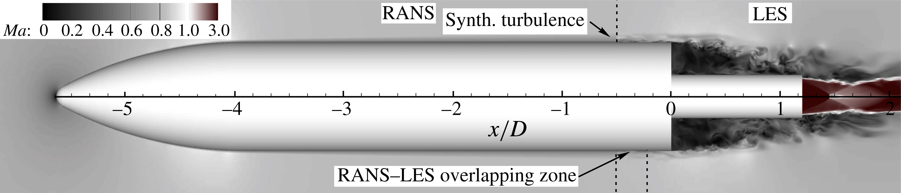
Flow decomposition into RANS and LES zones. The colour map shows the instantaneous Mach number distribution.

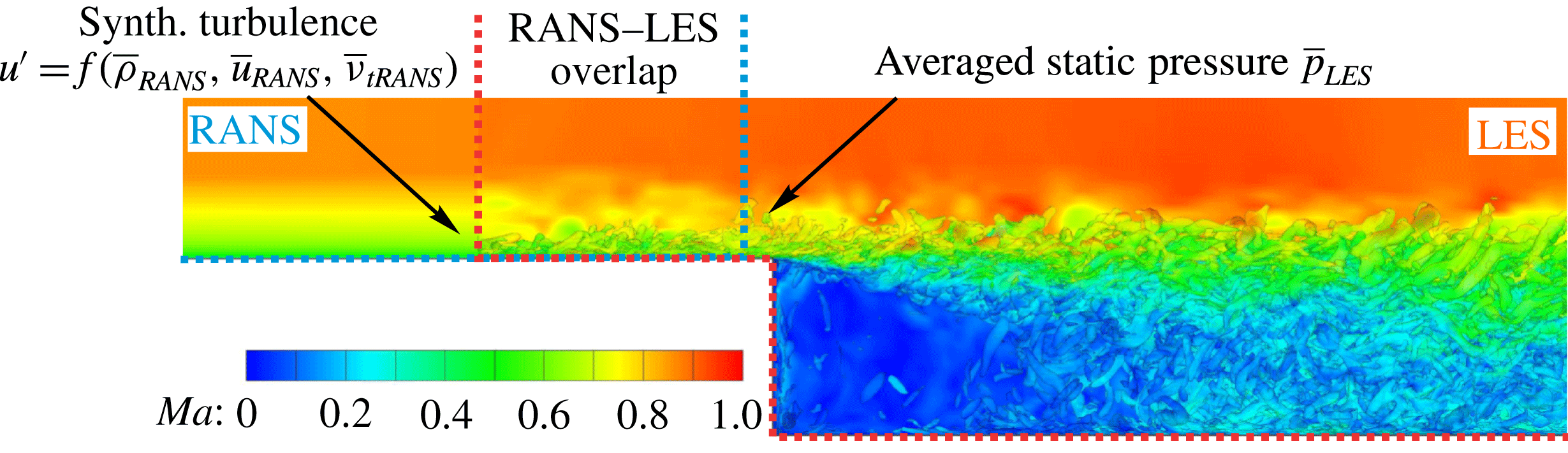
Bi-directional RANS–LES coupling using the reformulated synthetic turbulence generation method; coherent structures in the flow are visualized using
 $\unicode[STIX]{x1D706}_{2}$
-contours colour coded by the local Mach number.

The unsteady turbulent flow field around the generic space launcher configuration is computed using a zonal RANS–LES approach. As illustrated in figure 2, the computational domain is split into different zones according to the required turbulence modelling. That is, in the attached flow zones, i.e. around the main body and inside the nozzle, the turbulent flow field is predicted by solving the RANS equations, while in the wake region a LES is performed.
The computations are performed on a structured vertex-centred multi-block grid using an in-house zonal RANS–LES finite-volume flow solver. The Navier–Stokes equations of three-dimensional unsteady compressible flow are discretized in conservative form by a mixed centred upwind advective upstream splitting method (AUSM) scheme (Liou & Steffen Reference Liou and Steffen1993) with low numerical dissipation of second-order accuracy for the Euler terms and by a second-order accurate centred approximation for the non-Euler terms. The temporal integration is performed by an explicit five-stage Runge–Kutta method of second-order accuracy. The LES formulation is based on the monotone integrated LES (MILES) approach (Boris et al. Reference Boris, Grinstein, Oran and Kolbe1992) modelling the impact of the sub-grid scales by numerical dissipation. A detailed description of the fundamental LES solver is given by Meinke et al. (Reference Meinke, Schröder, Krause and Rister2002) and its convincing solution quality for fully turbulent sub- and supersonic flows is, e.g. discussed in Alkishriwi, Meinke & Schröder (Reference Alkishriwi, Meinke and Schröder2006) and Roidl, Meinke & Schröder (Reference Roidl, Meinke and Schröder2014). The RANS equations are discretized using the same overall discretization scheme. A one-equation turbulence model of Fares & Schröder (Reference Fares and Schröder2004) is employed to close the time-averaged equations.
The transition from the RANS to the LES zone is prescribed by applying a reformulated synthetic turbulence generation (RSTG) method by Roidl, Meinke & Schröder (Reference Roidl, Meinke and Schröder2013), Roidl et al. (Reference Roidl, Meinke and Schröder2014) that allows us to reconstruct the time-resolved turbulent fluctuations from the time-averaged upstream RANS solution, as illustrated in figure 3. The RSTG method is based on the synthetic eddy methods (SEM) of Jarrin et al. (Reference Jarrin, Benhamadouche, Laurence and Prosser2006) and Pamiès et al. (Reference Pamiès, Weiss, Garnier, Deck and Sagaut2009) and describes turbulence as a superposition of coherent structures. Those structures are generated over the LES inlet plane by superimposing virtual eddy cores which are defined in a virtual volume downstream of the inlet plane that has the streamwise, the wall normal and the spanwise dimensions of the local turbulent length scale, the boundary-layer thickness at the LES inlet and the spanwise extension of the computational domain. The turbulent length scales that describe the spatial properties of the synthetic structures depend on the distance from the wall and are derived from the local value of turbulent viscosity of the upstream RANS solution and scaled with the Reynolds number and the associated convection velocity. Having
 $N$
synthetic vortices, the fluctuating velocity signal is determined by the sum over all eddy cores
 $j$
 $$\begin{eqnarray}\displaystyle u_{i}^{\prime }(x)=\frac{1}{\sqrt{N}}\mathop{\sum }_{j=1}^{N}\unicode[STIX]{x1D700}_{j}\,f_{\unicode[STIX]{x1D70E}}(x-x_{j}), & & \displaystyle\end{eqnarray}$$
with
 $f_{\unicode[STIX]{x1D70E}}(x)$
being the shape function of the eddy, which is defined by a Gauss function implicitly meeting the two-point autocorrelation, and
 $\unicode[STIX]{x1D700}_{j}$
being a random number within the interval
 $[-1,+1]$
.
As a result, the final velocity signal is composed of an averaged velocity component
 $\overline{u_{i}}$
provided by the upstream RANS solution and the normalized fluctuations
 $u_{i}^{\prime }$
, which are subjected to a Cholesky decomposition
 $A_{mn}$
to assign the values of the Reynolds stress tensor corresponding to the turbulent eddy viscosity of the upstream RANS (Jarrin et al.
Reference Jarrin, Benhamadouche, Laurence and Prosser2006)
 $$\begin{eqnarray}\displaystyle u_{i}(x)=\overline{u_{i}}+A_{mn}u_{i}^{\prime }. & & \displaystyle\end{eqnarray}$$
At the end of the overlapping region, after a transition length of at least two boundary-layer thicknesses, the Reynolds-averaged static pressure computed from the LES field is imposed at the RANS outflow boundary to ensure a bi-directional, i.e. full, coupling of the zones via the exchanged flow variables. The same constant time step is used for both zones. The window width for Reynolds averaging is chosen larger than the high-frequency oscillations of the pressure field within the LES domain. Furthermore, an exponentially decaying sponge layer is used within the transition region on the main body. A detailed description of the method including the shape functions and length scale distributions is given in Roidl et al. (Reference Roidl, Meinke and Schröder2013).
2.3 Computational grids
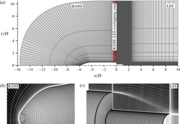
(a) Zonal grid topology (every fourth node shown); (b) RANS grid for the main body zone (every fourth node shown); (c) LES grid for the wake zone (every fourth node shown in the axial and radial and every eighth node shown in the azimuthal direction).

Within the framework of the zonal RANS–LES, a modular set-up is used for the simulation domain that consists of a RANS grid capturing the attached flow around the main body and an LES grid for the unsteady wake region. As shown in figure 4, the RANS section extends to approximately
 $10D$
away from the forebody walls in the wall-normal direction and ends at
 $x=-0.05D$
near the base shoulder located at
 $x=0$
, with
 $D$
being the diameter of the main body. The LES domain extends from
 $x=-0.5D$
to
 $10D$
in the streamwise and to
 $10.5D$
in the wall-normal direction. Thus, the RANS–LES transition plane is at
 $x=-0.5D$
upstream of the base shoulder with the boundary-layer thickness being
 $\unicode[STIX]{x1D6FF}=0.15D$
, which yields a sufficient transition length to a fully developed boundary layer of more than
 $3\unicode[STIX]{x1D6FF}$
, as required by the RSTG method. At the LES inflow plane inside the nozzle, which is at
 $x/D=1.1$
, i.e.
 $0.1D$
upstream of the nozzle exit, a time-averaged RANS profile obtained by a preceding axisymmetric two-dimensional RANS computation of the nozzle flow is used.
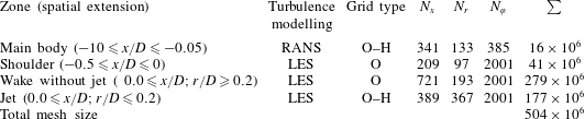
For the whole zonal set-up, approximately 500 million grid points are used. The numbers of the mesh points in each direction are listed in table 2, individually for each characteristic region of the computational domain. Note that for the main body and the jet flow regions, an O–H grid type is used due to the centreline singularity and consequently, the total number of the grid points for these two regions is less than the product of the three given dimensions.
The characteristic grid resolution for the RANS and LES zones within the transition region on the main body is given in table 3 in inner and outer coordinates. The number of the points resolving the boundary layer in the wall-normal direction is denoted by
 $N_{\unicode[STIX]{x1D6FF}}$
. The grid resolution satisfies typical mesh requirements for wall-bounded RANS and LES, respectively (Choi & Moin Reference Choi and Moin2012).
2.4 Computational resources
The time-resolved data are computed over a time interval of
 $409.6\,t_{ref}$
after a transient phase of
 $100\,t_{ref}$
, with
 $t_{ref}=D/u_{\infty }$
being the reference time unit needed by a particle moving with the free stream velocity
 $u_{\infty }$
to cover one reference length defined by the main body diameter. The computation has been performed on the CRAY XC40 system at the Stuttgart High Performance Computing Center with a peak performance of 7.42 Petaflops. In total, 14.6 million core hours distributed over 9600 cores via hybrid parallelization based on MPI, OpenMP and HDF5 have been used.
Mesh size overview for characteristic regions of the computational domain.

Wall resolution of the RANS and LES zones within the transition region (
 $-0.5\leqslant x/D^{\ast }\leqslant -0.05$
) in inner and outer coordinates;
 $l^{+}=u_{\unicode[STIX]{x1D70F}}/\unicode[STIX]{x1D708}$
, boundary-layer thickness
 $\unicode[STIX]{x1D6FF}$
defined by
 $\unicode[STIX]{x1D6FF}|_{x/D=-0.5}=0.15D$
.

3 Results
The discussion of the results is divided into three parts. First, the computed wake flow topology including the first- and second-order statistics is presented in detail and validated by experimental data. Next, the characteristic spatial and temporal scales of the wall pressure fluctuations and the resulting buffet loads are determined using methods of classical statistical analysis. Finally, the dynamic mode decomposition is used to identify and scrutinize the underlying coherent flow modes.
3.1 Wake flow topology and validation
The overall flow topology around the generic space launcher configuration computed by the zonal RANS–LES method is shown in figure 2 using Mach number contours. The incoming free stream with
 $Ma_{\infty }=0.8$
passes over the fairing of the model, locally accelerating to
 $Ma\approx 0.9$
and decelerating to
 $Ma_{\infty }\approx 0.8$
near the end of the forebody. The developed fully turbulent boundary layer separates at the axisymmetric shoulder at
 $x/D=0$
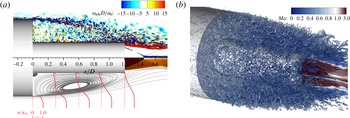
and forms a turbulent free-shear layer. This is indicated in the top part of figure 5(a) showing the instantaneous spanwise vorticity distribution in the wake. The shed shear layer rapidly evolves downstream of the separation due to the shear layer instability, causing the mixing layer and the turbulent structures to grow in size and intensity. This can be qualitatively identified in the development of the mean streamwise velocity profiles additionally shown in the lower part of figure 5(a) and in the plot of the Q-criterion (second invariant of the velocity gradient tensor) iso-surface in figure 5(b). Further downstream, the shear layer gradually approaches the nozzle and finally either impinges on its surface or passes over it, depending on the time instance and the azimuthal position, which will be discussed in detail in § 3.2.
Wake flow topology: (a) instantaneous spanwise vorticity distribution (top); time-averaged axial velocity profiles and streamlines (bottom); (b) turbulent structures in the wake visualized using the Q-criterion iso-surface (
 $Q\times a_{0}^{2}/D^{2}=300$
) colour coded by the Mach number.

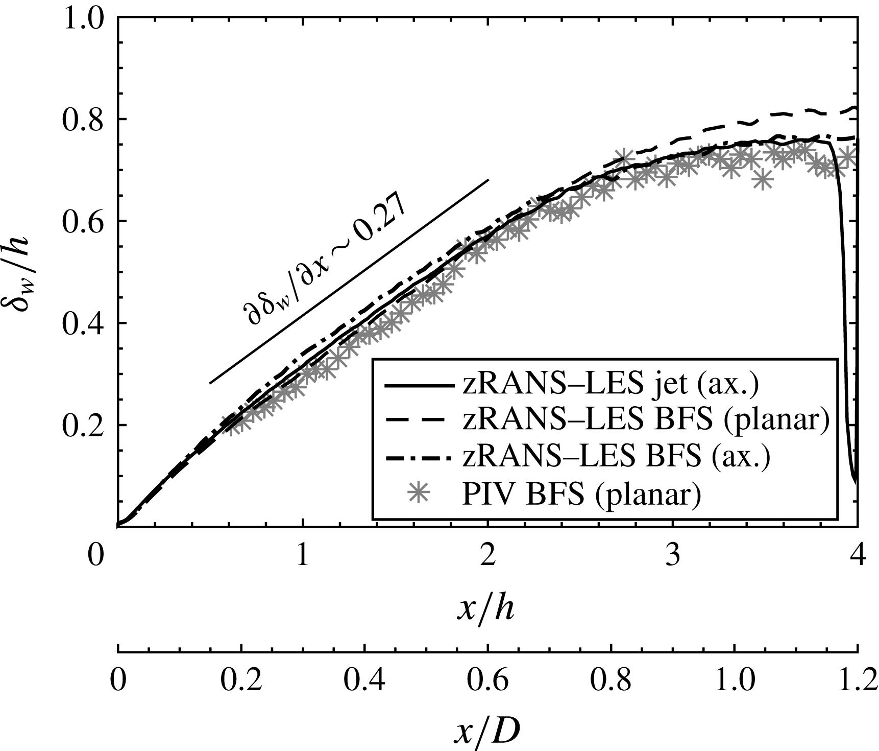
Streamwise evolution of the vorticity thickness in the wake region of the free-flight configuration (solid line) in comparison with an axisymmetric and planar backward-facing step (BFS) and experimental data.

To quantify the computed development of the turbulent shear layer, the streamwise evolution of the vorticity thickness (Brown & Roshko Reference Brown and Roshko1974) defined by
 $\unicode[STIX]{x1D6FF}_{w}(x)=(\bar{u}_{max}-\bar{u}_{min})/\text{max}(\unicode[STIX]{x2202}\bar{u}/\unicode[STIX]{x2202}y)$
is plotted in figure 6. Since for the investigated free-flight configuration no experimental data are directly available, a planar and an axisymmetric backward-facing step (BFS) configuration, previously investigated by the authors using the same numerical algorithm and discretization (Statnikov et al.
Reference Statnikov, Bolgar, Scharnowski, Meinke, Kähler and Schröder2016a
; Statnikov, Meinke & Schröder Reference Statnikov, Meinke and Schröder2016b
), is additionally depicted in figure 6 and compared to the experimental data kindly provided by the Bundeswehr University Munich. The comparison shows that in the initial range, i.e. for
 $0\leqslant x/h\lesssim 2.5$
with
 $h=0.3D$
being the step height, all three configurations feature the same linear growth rate of the vorticity thickness with
 $\unicode[STIX]{x1D6FF}_{w}^{\prime }=\unicode[STIX]{x2202}\unicode[STIX]{x1D6FF}_{w}/\unicode[STIX]{x2202}x\approx 0.27$
as a spreading rate measure, which agrees well with the experiment. Note that due to the synthetically generated turbulent fluctuations in the incoming boundary layer upstream of the separation, no artificial delay in the spatial development of the shed shear layer occurs, which would be observed if a classical detached-eddy simulation (DES) approach were applied (e.g. Deck & Thorigny Reference Deck and Thorigny2007; Pain et al.
Reference Pain, Weiss and Deck2014). The obtained value for
 $\unicode[STIX]{x1D6FF}_{w}^{\prime }$
coincides with the empirically derived estimate
 $\unicode[STIX]{x1D6FF}_{w}^{\prime }=0.18(1-r)/(1+r)$
for free planar shear layers given by Brown & Roshko (Reference Brown and Roshko1974), only if for the second stream the negative back flow is taken into account by the assumption
 $r=U_{2}/U_{1}\approx \bar{u}_{min}/U_{\infty }\approx -0.2$
. Without this correction, the current growth is
 $50\,\%$
larger than for a single jet shear layer determined by the velocity ratio
 $r=0$
. Thus, the recirculation region formed around the nozzle significantly amplifies the shear layer development by increasing the shear due to the reversed flow. In the immediate base region
 $x\approx 0$
, where
 $u_{min}\approx 0$
, the shear layer growth rate is even slightly higher, as known for example from canonical cavity flow problems (e.g. Rowley, Colonius & Basu Reference Rowley, Colonius and Basu2002; Larchevêque et al.
Reference Larchevêque, Sagaut, Lê and Comte2004), since turbulent structures are vertically reinjected into the mixing layer by the rotating field, which is illustrated by the streamlines additionally drawn in the lower part of figure 5(a).
Further downstream, i.e.
 $x/D\gtrsim 0.8$
(
 $x/h\gtrsim 2.6$
), the thickened shear layer interacts with the solid wall such that the initial linear quasi-free-shear layer growing behaviour is reduced and gradually flattens out with a plateau around
 $\unicode[STIX]{x1D6FF}_{w}\sim 0.7h$
. In the time-averaged flow field of the analysed free-flight Ariane 5-like configuration with an overexpanded jet, the shear layer reattaches onto the nozzle at
 $L_{r}=x_{r}/D=1.15$
. This can be seen in the streamline plot in the lower part of figure 5(a) and also corresponds to the drop of the vorticity thickness visible in figure 6. Notice that practically the same values for the mean reattachment position have been reported in the literature for similar generic configurations with the same nozzle-to-main body ratio, but without jet plume (Weiss et al.
Reference Weiss, Deck, Robinet and Sagaut2009; Weiss & Deck Reference Weiss and Deck2011) or with adapted jet (Deck & Thorigny Reference Deck and Thorigny2007). This indicates a reduced effect of the nozzle flow on the wake, at least as long as it is not strongly underexpanded, which is usually the case at transonic speeds (Statnikov et al.
Reference Statnikov, Sayadi, Meinke, Schmid and Schröder2015).
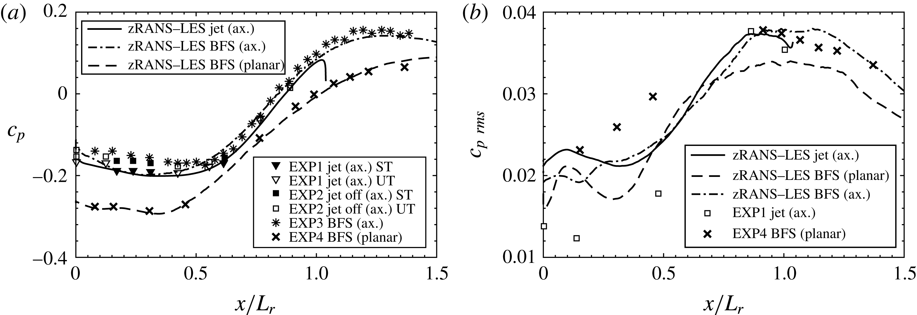
Streamwise distribution of the mean (a) and root-mean-square (b) wall pressure coefficient non-dimensionalized by the respective mean reattachment length. Comparison of the free-flight configuration with jet (
 $x/L_{r}=1.15D$
) with an axisymmetric (
 $x/L_{r}=1.3D$
) and planar (
 $x/L_{r}=2.1D^{\ast }$
) BFS as well as with experimental results (EXP1-EXP3: Deprés et al. (Reference Deprés, Reijasse and Dussauge2004), ST and UT denote steady and unsteady pressure transducers; EXP4: Statnikov et al. (Reference Statnikov, Bolgar, Scharnowski, Meinke, Kähler and Schröder2016a
)).

The shear layer separation at the main body shoulder is associated with a strong pressure drop at the base followed by a steep pressure increase near the reattachment position, which results in the base drag and structural loads on the lower wall. The resulting distribution of the mean and root-mean-square (r.m.s.) wall pressure coefficient along the separation region is shown in figure 7 and compared to several experimental results. As for the vorticity thickness, apart from the free-flight case, denoted as ‘jet (axisymmetric)’, distributions of two more BFS configurations denoted as ‘BFS (planar)’ and ‘BFS (axisymmetric)’ are plotted. According to Mabey (Reference Mabey1972), the streamwise direction is non-dimensionalized by the corresponding mean reattachment length values, which are defined in the caption of figure 7. The comparison for the mean wall pressure coefficient in figure 7(a) illustrates an excellent agreement between the zonal computations and the experiments. Furthermore, a stronger pressure deficit for the planar wake compared to the axisymmetric distributions is visible. This is consistent with the well-known fact of larger drag coefficients for quasi two-dimensional shapes than for their axisymmetric counterparts, e.g. circular cylinders versus spheres or blunt wedges versus cones. The streamwise distribution of
 $c_{p\,rms}$
is shown in figure 7(b). Taking into account higher sensitivities of the second-order statistics to intrinsic uncertainties in experiments and simulations, e.g. free stream turbulence and noise levels of the wind tunnels, the computed streamwise distribution of the wall pressure fluctuations can be considered of satisfactory quality for all cases and within the scattering range of the experimental data. As expected (Mabey Reference Mabey1972), the highest wall pressure fluctuations and thus dynamic loads occur slightly upstream of the mean reattachment position, with a wide streamwise extension of the corresponding peaks indicating large-scale oscillations within the reattachment region. This aspect will be discussed in the next subsection.
3.2 Statistical analysis of wall pressure fluctuations and buffet loads
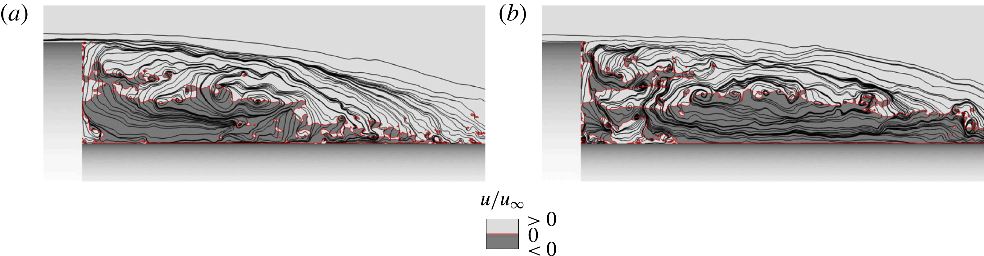
Instantaneous streamlines in the near wake shown in the azimuthal plane
 $\unicode[STIX]{x1D711}=0^{\circ }$
for two time samples
 $t_{1}$
(a) and
 $t_{2}$
(b). The darker grey level denotes backflow regions.

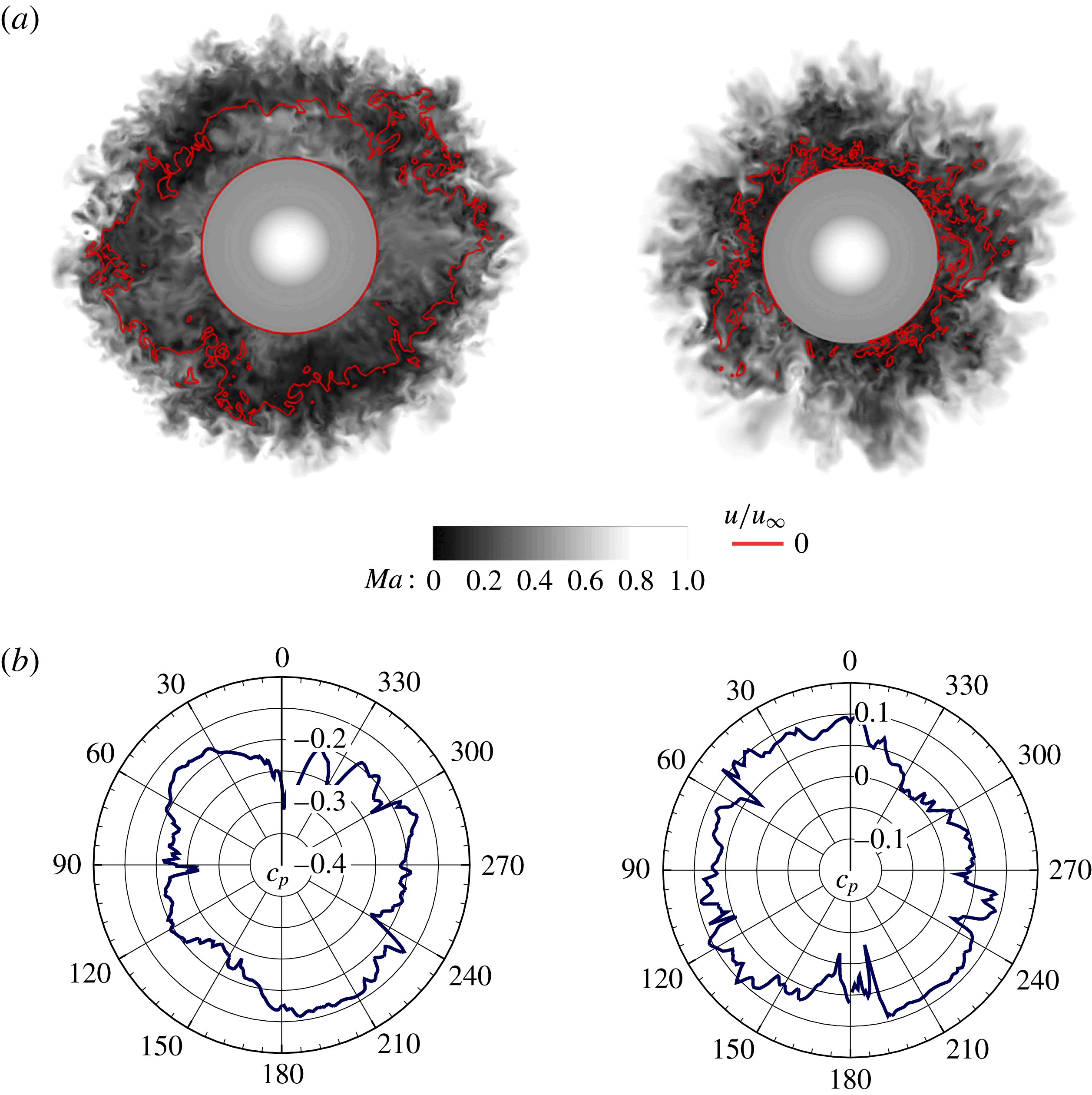
Instantaneous Mach number distribution (a) and corresponding polar plots of the pressure coefficient (b) in two cross-sections positioned at the nozzle centre
 $x/D=0.6$
(left) and the mean reattachment positions
 $x/D=1.15$
(right).

The wake flow of the investigated free-flight configuration is highly dynamic and is characterized by a manifold of spatio-temporal structures. For instance, the instantaneous streamline snapshots taken at the same azimuthal position
 $\unicode[STIX]{x1D711}=0$
at two time samples show in figure 8 that sometimes the shear layer reattaches onto the nozzle close to its centre more than one step height upstream of the mean reattachment position or it does not reattach onto the nozzle passing over it. Besides, the recirculation region incorporates a manifold of large-scale spanwise vortices of different sizes such that the time-averaged topology with only two toroidal vortices, illustrated in figure 5(a), can be hardly identified. Furthermore, despite the axisymmetric geometry and zero angle of attack, the shed shear layer approaches the nozzle not axisymmetrically resulting in a pronounced asymmetry of the induced instantaneous azimuthal pressure distribution. This is evidenced by the instantaneous Mach number distribution and the corresponding polar plots of the pressure coefficient shown in figure 9 for two cross-sections positioned at the nozzle centre
 $x/D=0.6$
and the mean reattachment position
 $x/D=1.15$
.
3.2.1 Spatio-temporal spectral analysis of wall pressure fluctuations
To provide insight into the temporal periodicity aspects of the wall pressure fluctuations, the power spectral density (PSD) distribution of the wall pressure signals is computed at several streamwise positions. The PSD function of the analysed data sequence consisting of
 $4096$
time instances equidistantly sampled with
 $\unicode[STIX]{x0394}t=0.1D/u_{\infty }$
(see § 2.4 for details) is computed using Welch’s algorithm with Hanning windowing of 512 samples each and 50 per cent overlapping. To account for the detected spanwise variation, the pressure signals are analysed at 500 positions equidistantly distributed over
 $360^{\circ }$
(
 $\unicode[STIX]{x0394}\unicode[STIX]{x1D711}=0.72^{\circ }$
) and subsequently averaged in the frequency domain. The non-dimensional frequency is defined by the Strouhal number
 $Sr_{D}=fD/u_{\infty }$
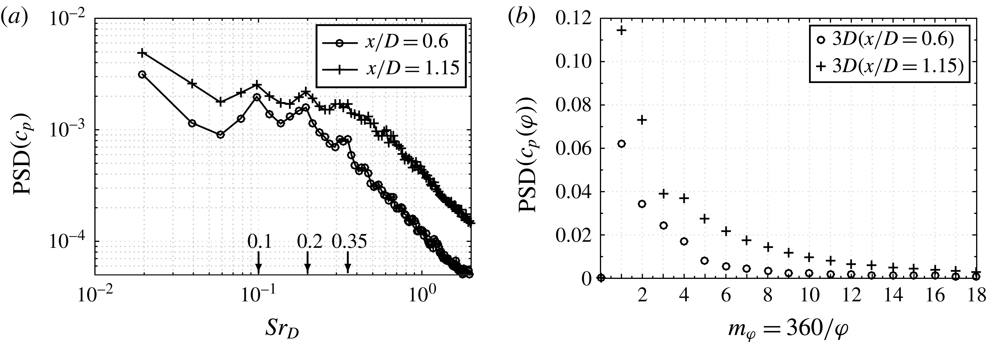
based on the main body diameter and the free stream velocity. Figure 10(a) shows the obtained spectra for the two previously defined characteristic positions, i.e. at the nozzle centre (
 $x/D=0.6$
) and the mean reattachment position
 $x/D=1.15$
. At both streamwise positions, two distinct peaks around
 $Sr_{D}\approx 0.1$
and
 $Sr_{D}\approx 0.2$
as well as a local broadband plateau at
 $Sr_{D}\approx 0.35\pm 0.05$
can be identified.
Spatio-temporal spectral analysis of wall pressure fluctuations
 $c_{p^{\prime }}$
on the nozzle: (a) power spectral density (PSD); (b) spatial PSD in the azimuthal wavenumber domain.

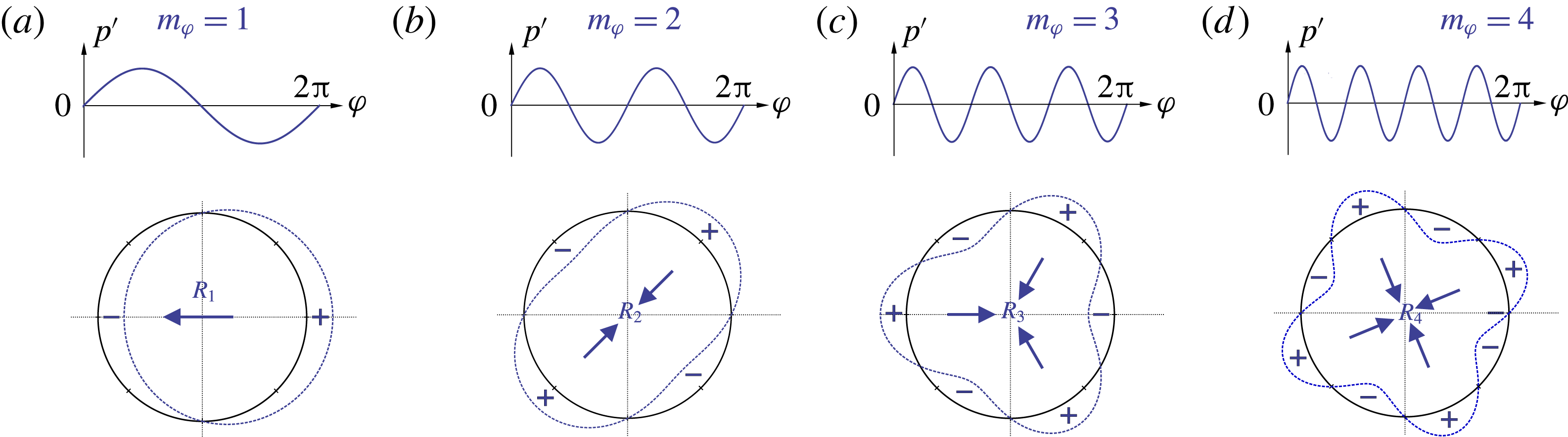
Schematic interpretation of the first four non-axisymmetric azimuthal pressure modes in terms of resulting loads on the nozzle segment.

Furthermore, to analyse the azimuthal coherency of the non-axisymmetric pressure distribution, the spatial PSD function of the transposed space–time data matrix of the previously analysed pressure values is computed. Thus, for each of 4096 time samples the azimuthal pressure distribution given by 500 points is projected into the wavenumber domain using Welch’s algorithm and subsequently averaged to account for the temporal variation. Due to the natural
 $2\unicode[STIX]{x03C0}$
-periodicity of each pressure sample
 $c_{p}(\unicode[STIX]{x1D711})$
, no window function and no overlapping is used. Figure 10(b) shows the obtained spatial PSD for the same two characteristic streamwise positions as before. The presence of a dominant antisymmetric
 $m_{\unicode[STIX]{x1D711}}=1$
mode is clearly visible that is followed by higher wavenumber modes with continuously descending amplitudes. As schematically visualized in figure 11, the dominant
 $m_{\unicode[STIX]{x1D711}}=1$
mode causes most critical side loads on the nozzle structure at the analysed streamwise position, while the higher wavenumber modes correspond to ovalization or buckling loads, i.e. modes
 $m_{\unicode[STIX]{x1D711}}=2$
or
 $m_{\unicode[STIX]{x1D711}}\geqslant 3$
.
3.2.2 Buffet loads
(a) Scatter plot of the instantaneous side loads on the nozzle structure in polar coordinates with the
 $\unicode[STIX]{x1D6FC}=95$
confidence ellipse drawn by dashed red line; (b) premultiplied normalized power spectral density (
 $f\times \text{PSD}/\unicode[STIX]{x1D70E}^{2}$
) of the side load components (
 $\unicode[STIX]{x1D70E}_{c_{FY}}=4.9\times 10^{-3}$
,
 $\unicode[STIX]{x1D70E}_{c_{FZ}}=5.1\times 10^{-3}$
).

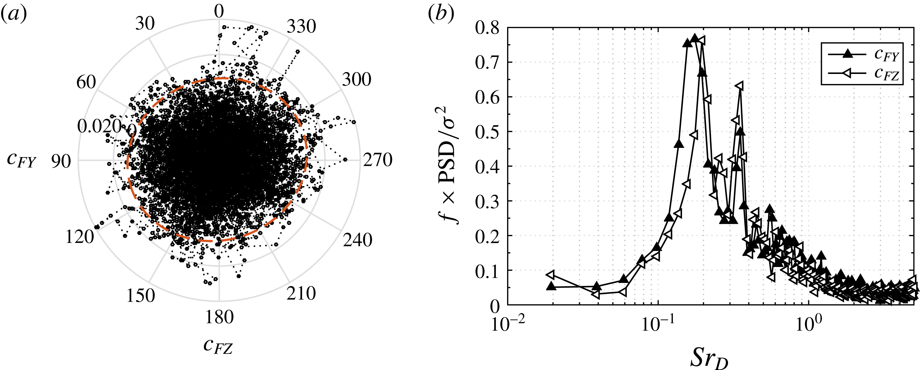
The instantaneous buffet load is computed by the surface integral of the instantaneous wall pressure field on the nozzle, neglecting the azimuthal component of the viscous stresses due to their significantly smaller amplitudes. The vectors of the instantaneous side force coefficients are shown in figure 12(a) in polar coordinates, with
 $c_{FY}$
and
 $c_{FZ}$
denoting their Cartesian components non-dimensionalized by the dynamic pressure
 $q_{\infty }=(\unicode[STIX]{x1D6FE}/2)Ma^{2}p_{\infty }$
and the main body cross-section area
 $A_{ref}=\unicode[STIX]{x03C0}D^{2}/4$
. It is seen that the orientation of the side load vector is random and isotropic, which is evidenced by practically axisymmetric shape of the
 $\unicode[STIX]{x1D6FC}=95$
confidence ellipse encompassing
 $95\,\%$
of the computed values additionally drawn in the scatter plot. This is consistent with the axisymmetric geometry and inflow conditions.
Despite the spatial isotropy, the buffet loads, however, feature a pronounced temporal periodicity. Figure 12(b) shows the frequency-premultiplied normalized PSD function for the two Cartesian components of the side force coefficient to allow a geometric interpretation of the total energy distribution of the fluctuating force by the area under the curve, which follows from the relation
 $\unicode[STIX]{x1D70E}^{2}=\int _{0}^{\infty }G(f)\,\text{d}f=\int _{0}^{\infty }f\times G(f)\,\text{d}(\log f)$
between the signal variance and the power spectral density distribution
 $G(f)$
over the frequency
 $f$
. Consistent with the axisymmetric geometry and inflow, almost identical spectra are obtained for the both Cartesian components. The slight deviations are caused by the limited signal length. One energetically most dominant frequency range at
 $Sr_{D}\approx 0.2$
is clearly seen. There is another pronounced but narrower and consequently, energetically less strong range around
 $Sr_{D}\approx 0.35$
. Notice that these frequencies correlate with the respective values in the wall pressure fluctuations shown in figure 10(a), while the low-frequency peaks around
 $Sr_{D}\approx 0.1$
detected previously are hardly visible.
Path of the side load during two characteristic time intervals of
 $T=5D/u_{\infty }$
in polar coordinates with the
 $\unicode[STIX]{x1D6FC}=95$
confidence ellipses drawn by dashed red lines.

The identified characteristic frequencies of wall pressure fluctuations and resulting buffet loads are consistent with the experimental and numerical results reported in the literature for similar space launcher configurations (e.g. Deprés et al.
Reference Deprés, Reijasse and Dussauge2004; Meliga & Reijasse Reference Meliga and Reijasse2007; Weiss et al.
Reference Weiss, Deck, Robinet and Sagaut2009; Weiss & Deck Reference Weiss and Deck2011; Pain et al.
Reference Pain, Weiss and Deck2014). A conventional statistical analysis, however, cannot provide direct information on the underlying dynamic modes hidden in the multiple spatio-temporal scales of turbulence, which is why the attribution of the identified frequencies to certain coherent flow patterns is a particularly difficult task. For example, as briefly mentioned in the introduction, a large uncertainty exists regarding the true three-dimensional shape of the energetically most relevant antisymmetric mode at
 $Sr_{D}\approx 0.2$
, which is mainly associated with the buffet phenomenon. Widely spread is the assumption of a helical vortical structure in the wake of an axisymmetric body that is responsible for periodic side loads and simultaneously maintains the overall axisymmetry of the time-averaged flow field (e.g. Deprés et al.
Reference Deprés, Reijasse and Dussauge2004; Meliga & Reijasse Reference Meliga and Reijasse2007; Weiss et al.
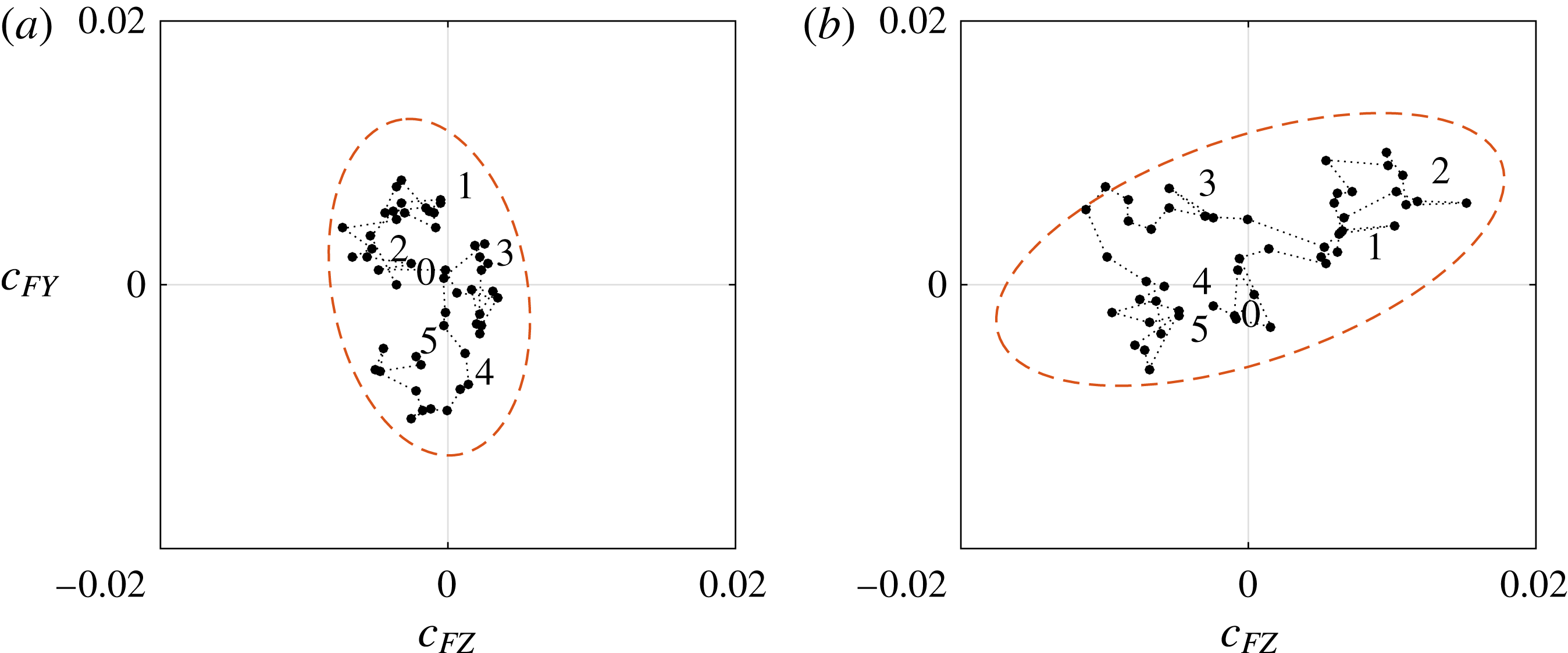
Reference Weiss, Deck, Robinet and Sagaut2009). Besides the fact that, to the best of the authors’ knowledge, such a mode has not been visualized yet, this assumption also appears controversial for several reasons. Firstly, the existence of one helical mode in the wake of an axisymmetric and not spinning body interferes with the Kelvin’s vortex theorem in planes normal to the main flow direction. Secondly, a helical mode would result in a pronounced azimuthal rotation of the side load vector rather than in the change of its amplitude. However, by closely following the path development of the side load vector drawn in polar coordinates during the characteristic time intervals of
 $T=5Du_{\infty }$
defined by the inverse of the characteristic frequency
 $Sr_{D}=0.2$
, no traces of a periodic helical mode are visible. On the contrary, as illustrated in figure 13 by two segmented time intervals, the side load oscillations appear to be trapped in a randomly oriented elongated ellipse that changes its azimuthal orientation irregularly, resulting in the spatial isotropy of the side load with a zero mean, as was shown in figure 12(a). This large uncertainty about the true three-dimensional shape of the wake flow modes associated with the well-known characteristic frequencies clearly shows that an additional analysis is required, which is done by means of the following dynamic mode decomposition.
3.3 Reduced-order analysis
We turn now to a reduced-order analysis based on optimized DMD (Schmid Reference Schmid2010). Before a detailed discussion of the obtained results in the second subsection, first a brief introduction into DMD is given.
3.3.1 DMD formalism
DMD is a data-driven decomposition technique to extract spatio-temporal dynamic information in the form of spatial modes with their specific frequencies and growth/decay rates from multi-dimensional field data collected from time-resolved simulations or experiments. Thus, a high-dimensional flow field
 $\unicode[STIX]{x1D66B}(x,y,z,t)$
can be decomposed into a set of complex spatial dynamic modes
 $\unicode[STIX]{x1D753}_{n}(x,y,z)\in \mathbb{C}^{3}$
with respective amplitudes
 $a_{n}\in \mathbb{C}$
and frequencies
 $\unicode[STIX]{x1D706}_{n}\in \mathbb{C}$
, i.e.
 $$\begin{eqnarray}\displaystyle \unicode[STIX]{x1D66B}(x,y,z,t)=\mathop{\sum }_{n=1}^{N}a_{n}\exp (\unicode[STIX]{x1D706}_{n}t)\unicode[STIX]{x1D753}_{n}(x,y,z). & & \displaystyle\end{eqnarray}$$
Applied to the data from time-resolved simulations or experiments, the flow field
 $\unicode[STIX]{x1D66B}(x,y,z,t)$
is discretized as a sequence of
 $N$
equidistantly sampled snapshot vectors
 $\boldsymbol{v}_{i}(x,y,z)\in \mathbb{R}^{M}$
column wise assembled into a vast snapshot matrix
 $\unicode[STIX]{x1D651}_{1}^{N}\in \mathbb{R}^{M\times N}$
as an input, where the subscript denotes the first and the superscript the last time instance in the set. The decomposition described by (3.1) can then be represented in a general matrix form
 $$\begin{eqnarray}\displaystyle \underbrace{[\boldsymbol{v}_{1},\boldsymbol{v}_{2},\ldots ,\boldsymbol{v}_{N}]}_{\unicode[STIX]{x1D651}_{1}^{N}}=\underbrace{[\unicode[STIX]{x1D753}_{1},\unicode[STIX]{x1D753}_{2},\ldots ,\unicode[STIX]{x1D753}_{N}]}_{\unicode[STIX]{x1D731}}\underbrace{\left(\begin{array}{@{}cccc@{}}a_{1} & & & \\ & a_{2} & & \\ & & \ddots & \\ & & & a_{N}\end{array}\right)}_{\unicode[STIX]{x1D63F}_{a}=\text{diag}\{a\}}\underbrace{\left(\begin{array}{@{}cccc@{}}1 & \unicode[STIX]{x1D707}_{1} & \cdots \, & \unicode[STIX]{x1D707}_{1}^{N}\\ 1 & \unicode[STIX]{x1D707}_{2} & \cdots \, & \unicode[STIX]{x1D707}_{2}^{N}\\ \vdots & \vdots & \ddots & \vdots \\ 1 & \unicode[STIX]{x1D707}_{N} & \cdots \, & \unicode[STIX]{x1D707}_{N}^{N}\end{array}\right)}_{\unicode[STIX]{x1D651}_{and}},\quad & & \displaystyle\end{eqnarray}$$
where the temporal evolution of the modes is given, in discrete time, by the Vandermonde matrix
 $\unicode[STIX]{x1D651}_{and}$
filled with the geometrical progression of the so-called Ritz eigenvalues
 $\unicode[STIX]{x1D707}_{n}$
related with the frequency of the DMD modes
 $\unicode[STIX]{x1D706}_{n}$
via
 $$\begin{eqnarray}\displaystyle \unicode[STIX]{x1D707}_{n}=\exp (\unicode[STIX]{x1D706}_{n}\unicode[STIX]{x0394}t). & & \displaystyle\end{eqnarray}$$
In this work, the set of complex quantities
 $\{\unicode[STIX]{x1D753}_{n},a_{n},\unicode[STIX]{x1D707}_{n}\}$
describing the system dynamics is determined using the optimized DMD approach presented in Schmid (Reference Schmid2010). Accordingly, a preprocessing step based on a singular value decomposition (SVD) of the snapshot matrix
 $\unicode[STIX]{x1D651}_{1}^{N-1}=\unicode[STIX]{x1D650}\unicode[STIX]{x1D72E}\unicode[STIX]{x1D652}^{\ast }$
is used to compute an economy size DMD matrix
 $\widetilde{\unicode[STIX]{x1D64E}}\equiv \unicode[STIX]{x1D650}^{\star }\unicode[STIX]{x1D651}_{2}^{N}\unicode[STIX]{x1D652}\unicode[STIX]{x1D72E}^{-1}$
. It can also be shown that
 $\widetilde{\unicode[STIX]{x1D64E}}=\unicode[STIX]{x1D650}^{\ast }\unicode[STIX]{x1D63C}\unicode[STIX]{x1D650}$
, which implies that the DMD matrix
 $\widetilde{\unicode[STIX]{x1D64E}}$
corresponds to an optimal low-dimensional representation of the vast unknown inter-snapshot operator
 $\unicode[STIX]{x1D63C}\in \mathbb{C}^{M\times M}$
, which defines the temporal evolution of the system via
 $\boldsymbol{v}_{i+1}=\unicode[STIX]{x1D63C}\boldsymbol{v}_{i}$
, on the subspace spanned by its POD modes. The crucial SVD preprocessing step reduces the problem dimensions from
 $M^{2}$
to
 $(N-1)^{2}$
for
 $M>>N$
and significantly improves the numerical condition.
The eigenvalue decomposition (EVD) of the DMD matrix
 $\widetilde{\unicode[STIX]{x1D64E}}\unicode[STIX]{x1D654}=\unicode[STIX]{x1D741}\unicode[STIX]{x1D654}$
yields the sought Ritz eigenvalues
 $\unicode[STIX]{x1D707}_{n}$
and Ritz eigenvectors
 $\boldsymbol{Y}_{n}$
defining the DMD modes via the relation
 $\unicode[STIX]{x1D731}=\unicode[STIX]{x1D650}\unicode[STIX]{x1D654}$
. The decomposition is completed by minimizing the objective function
 $$\begin{eqnarray}\displaystyle \underset{a}{\text{minimize}}\;\Vert \unicode[STIX]{x1D651}_{1}^{N}-\unicode[STIX]{x1D731}\unicode[STIX]{x1D63F}_{a}\unicode[STIX]{x1D651}_{and}\Vert _{F}^{2}, & & \displaystyle\end{eqnarray}$$
with
 $\Vert \cdot \Vert _{F}$
being the Frobenius norm, to determine the amplitudes
 $a_{n}$
, which results in a convex optimization problem and can be solved using standard methods (e.g. Boyd & Vandenberghe Reference Boyd and Vandenberghe2004). For more algorithmic details, the reader is referred to Schmid (Reference Schmid2010) and Jovanović et al. (Reference Jovanović, Schmid and Nichols2014).
3.3.2 DMD spectrum
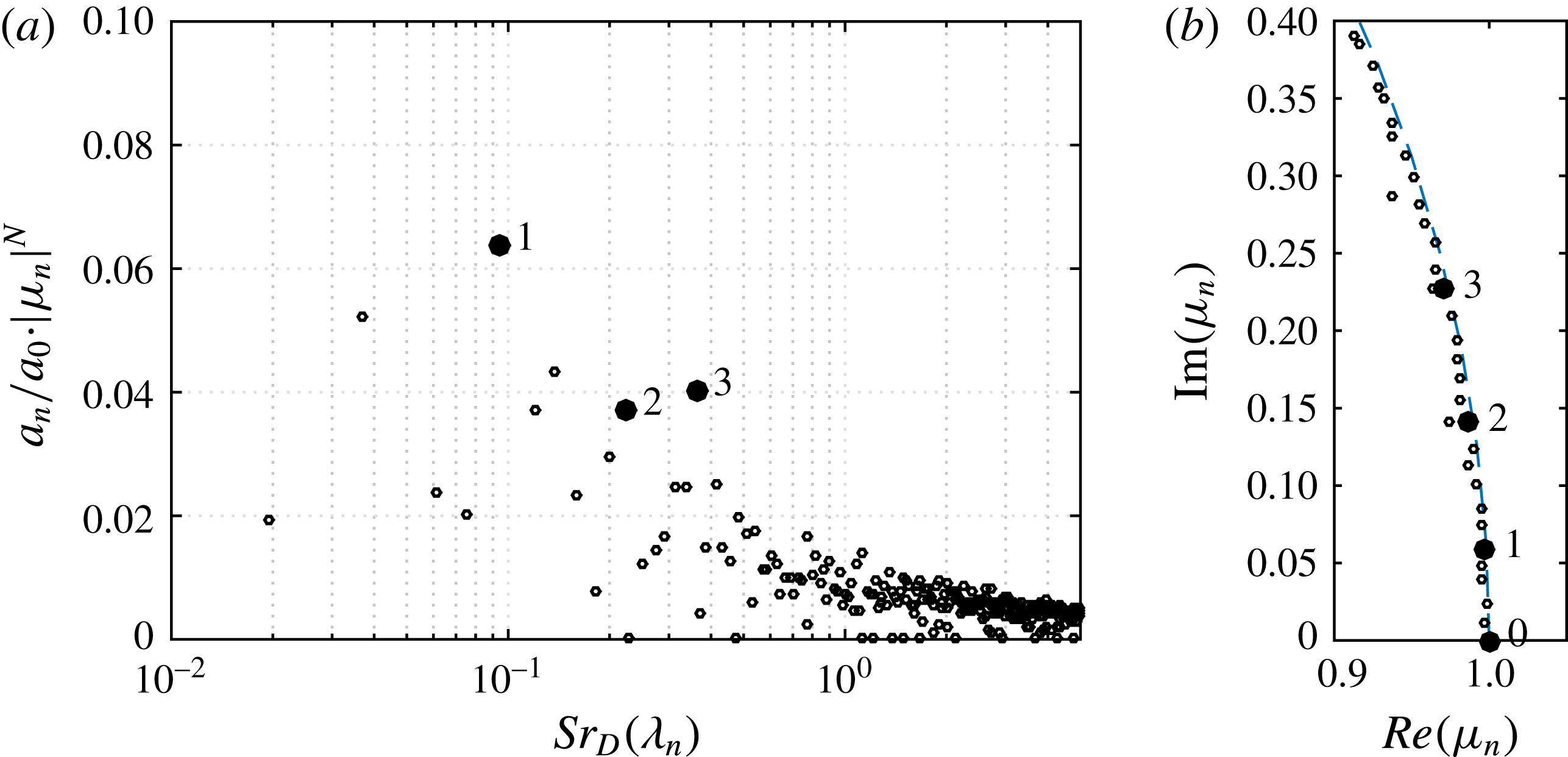
Normalized DMD spectrum of the velocity and pressure field in the physical frequency domain (a); Ritz eigenvalues
 $\unicode[STIX]{x1D707}_{n}=\exp (\unicode[STIX]{x1D706}_{n}\unicode[STIX]{x0394}t)$
of the low-frequency region of interest plotted with respect to the unit circle (b).

The optimized DMD algorithm by Schmid (Reference Schmid2010) has been integrated into the post-processing routine of the in-house zonal flow solver. The following DMD results are based on the analysis of 512 snapshots of the three-dimensional pressure and velocity field equidistantly distributed with
 $\unicode[STIX]{x0394}t=0.1D/u_{\infty }$
. Thus, the DMD input corresponds to the same window length and sampling frequency as used for the spectral analyses in the previous section. Using the full spatial resolution, however, would result in a snapshot matrix with a total number of elements of the order of
 $10^{15}$
, which is why the number of the mesh points taken into account for the modal analysis was reduced by skipping every second point in the streamwise and radial direction, and every fourth in the azimuthal. Furthermore, as recommended by Schmid (Reference Schmid2010), the domain was restricted to the immediate region of interest to improve the numerical condition and to further reduce the number of the cells. In spite of this reduction, each snapshot contains
 $16.5\times 10^{6}$
cells and requires 650 MB of storage in double precision format. To handle the resulting large matrices, the DMD algorithm has been parallelized using MPI, HDF5, and ScaLAPACK to be run on the CRAY XC40 system at the Stuttgart High Performance Computing Center. It takes approximately 400 core hours typically distributed over 2400 cores for the post-processing set-up described above.
The computed DMD spectrum is shown in figure 14(a) and presents the distribution of the amplitudes
 $a_{n}$
of the individual DMD modes
 $\unicode[STIX]{x1D753}_{n}$
over the non-dimensional physical frequency
 $Sr_{D}(\unicode[STIX]{x1D706}_{n})$
that is given by the imaginary part of the complex frequency
 $\unicode[STIX]{x1D706}_{n}=\unicode[STIX]{x1D706}_{r}+\text{i}\unicode[STIX]{x1D706}_{i}$
according to the relation
 $Sr(\unicode[STIX]{x1D706}_{n})=\unicode[STIX]{x1D706}_{i}/2\unicode[STIX]{x03C0}$
. Notice that, similar to the Fourier transform, the DMD modes along with their frequencies and the amplitudes appear as pairs of complex conjugates, which reduces the obtained number of the degrees of freedom by a factor of two and indirectly yields the Nyquist criterion. Moreover, each complex conjugate pair of eigenvalues contains the same frequency and decay rate information, such that a one-sided representation of the spectrum is used. Furthermore, the amplitudes
 $a_{n}$
are additionally normalized by the mean mode amplitude
 $a_{0}$
and multiplied by the respective damping
 $|\unicode[STIX]{x1D707}_{n}|^{-N}=|\text{exp}(\unicode[STIX]{x1D706}_{n}\unicode[STIX]{x0394}t)|^{-N}$
to account for transient modes which appear with artificially high amplitudes
 $a_{n}$
, but feature a high decay rate and do not contribute appreciably to the overall processed data sequence. A decaying transient mode is characterized by a complex Ritz eigenvalue
 $\unicode[STIX]{x1D707}_{n}=r_{n}\text{e}^{\text{i}\unicode[STIX]{x1D703}_{n}}$
with an amplitude
 $r\ll 1$
. This property follows, e.g. from (3.2), showing that the temporal evolution of the flow field is described by the Vandermonde matrix which contains the geometric progression of the respective complex eigenvalues, i.e.
 $\unicode[STIX]{x1D707}^{t}=r^{t}\text{e}^{\text{i}t\unicode[STIX]{x1D703}}$
for
 $t=\{1\ldots N\}$
. Thus, the transient Ritz eigenvalues clearly lie inside the unit circle, as illustrated in figure 14(b), where for the sake of clarity only the low-frequency eigenvalues of interest are shown on the corresponding segment of the unit circle. On the whole, three most stable dynamic modes of interest, frequencies of which closely match the characteristic peaks in the wall pressure spectra and side loads, are identified and marked by filled black circles, i.e.
 $Sr_{D}(\unicode[STIX]{x1D706}_{1})\approx 0.1$
,
 $Sr_{D}(\unicode[STIX]{x1D706}_{2})\approx 0.2$
and
 $Sr_{D}(\unicode[STIX]{x1D706}_{3})\approx 0.35$
. The shape of these modes contains the information about the underlying phase-averaged coherent modulation of the flow field and is analysed in the following.
3.3.3 Reduced-order analysis based on DMD results
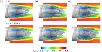
Reduced-order modelled streamwise velocity field for the three characteristic frequencies: (a)
 $Sr_{D}(\unicode[STIX]{x1D706}_{1})\approx 0.1$
, (b)
 $Sr_{D}(\unicode[STIX]{x1D706}_{2})\approx 0.2$
, (c)
 $Sr_{D}(\unicode[STIX]{x1D706}_{3})\approx 0.35$
. Time instances at the beginning (top) and in the middle (bottom) of the respective period are shown.

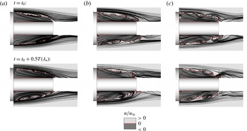
Streamline plots of the reduced-order modelled composite velocity field for the three characteristic frequencies: (a)
 $Sr_{D}(\unicode[STIX]{x1D706}_{1})\approx 0.1$
, (b)
 $Sr_{D}(\unicode[STIX]{x1D706}_{2})\approx 0.2$
, (c)
 $Sr_{D}(\unicode[STIX]{x1D706}_{3})\approx 0.35$
. The darker grey level in the field denotes backflow regions. Time instances at the beginning (top) and in the middle (bottom) of the respective period are shown.

The coherent phase-averaged fluid motion is obtained by superimposing the steady mean mode
 $\unicode[STIX]{x1D753}_{0}$
with the complex conjugate pair of the respective dynamic modes at the given frequency and subsequently reconstructing the temporal modulation of the flow field according to (3.2). The resulting reduced-order three-dimensional streamwise velocity fields are shown in figure 15 for the three frequencies of interest in ascending order, i.e.
 $Sr_{D}(\unicode[STIX]{x1D706}_{1})\approx 0.1$
(a),
 $Sr_{D}(\unicode[STIX]{x1D706}_{2})\approx 0.2$
(b),
 $Sr_{D}(\unicode[STIX]{x1D706}_{3})\approx 0.35$
(c). The first (top) row of the subplots shows the time instance
 $t_{0}$
, while the second (bottom) row illustrates the time instances
 $t_{0}+0.5T(\unicode[STIX]{x1D706}_{n})$
, i.e. after one half of the respective period defined by
 $T(\unicode[STIX]{x1D706}_{n})=Sr_{D}(\unicode[STIX]{x1D706}_{n})^{-1}D/u_{\infty }$
, to visualize the temporal evolution of the spatial modulation. For a more dynamic impression, the reader should view the supplementary movies which are available online at https://doi.org/10.1017/jfm.2017.46. Three types of coherent fluid motion are identified. The spatio-temporal modulation of the velocity field at
 $Sr_{D}\approx 0.1$
(figure 15
a) indicates a longitudinal pumping motion of the recirculation region. At the second frequency of interest,
 $Sr_{D}\approx 0.2$
(figure 15
b), a pronounced antisymmetric cross-flapping motion of the shear layer is clearly seen. At the third frequency,
 $Sr_{D}\approx 0.35$
(figure 15
c), a quasi-swinging motion of the shear layer is extracted that occurs in phase with the previous flapping mode.
To provide further insight into the origin of the identified wake dynamics, projected streamline plots of the reconstructed reduced-order modelled velocity fields are shown in figure 16 using the previous subfigure layout, i.e. the columns correspond to the three frequencies in ascending order, while the rows show the time instances at the begin and in the middle of the respective period. Again, for a more dynamic impression, the reader should view the supplementary movies which are available online. A close look at the temporal evolution of the streamlines reveals that the longitudinal pumping motion at
 $Sr_{D}\approx 0.1$
shown in figure 16(a) is, in fact, a harmonic oscillation of the main recirculation vortex in the streamwise direction with a pronounced antisymmetry. Therefore, for the remainder of the discussion it will be denoted as longitudinal cross-pumping mode. The next column of the streamline plots, figure 16(b), corresponds to the mode at
 $Sr_{D}\approx 0.2$
and reveals an antisymmetric vortex shedding. Interestingly, the factor of two between the frequency values of the pumping and shedding modes becomes logical when considering their in-phase relation that is visible in the streamline plots. Thus, each time when the main vortex is close to the nozzle exit as a result of the longitudinal cross-pumping motion, a vortical structure is shed from the recirculation region. This happens twice during one cross-pumping period, once on one side and once on the opposite side, which convincingly explains the initially unknown connection between the frequency values of the two peaks detected in the wall pressure spectra. At the last frequency of interest,
 $Sr_{D}\approx 0.35$
, the identified shear layer swinging motion is caused by the shedding of smaller vortices and is quasi a higher harmonic of the main vortex shedding mode.
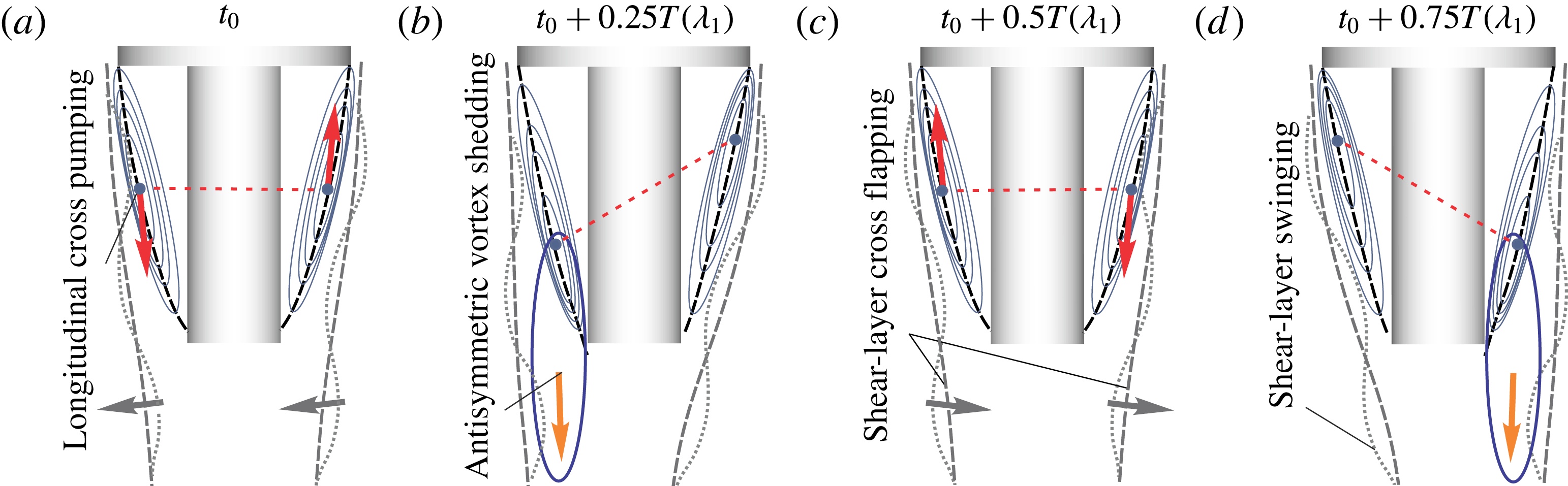
Schematic representation of the reduced-order modelled coherent fluid motion in the wake during one characteristic time period of
 $T(\unicode[STIX]{x1D706}_{1})=10D/u_{\infty }$
.

To sum up the results of the reduced-order analysis of the velocity field, the identified modes of the wake dynamics, each of which is associated with a single characteristic frequency, are schematically shown in figure 17. Note that the straightforward identification of the coherent fluid motion is available only due to the optimal phase-averaging approach of DMD, since the original non-decomposed wake field is characterized by a manifold of different spatial and temporal scales, as can be clearly pictured comparing the streamline plots of the reduced-order modelled field shown in figure 16 with those before the decomposition illustrated in figure 8.
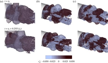
Next, the three-dimensional pressure modes in the wake are analysed. For this purpose, the reduced-order spatio-temporal modulation of the pressure field at a selected frequency is obtained via (3.2) as for the velocity field before. The only difference is that the mean pressure mode is not taken into account due to the low level of pressure fluctuations compared to the mean value. The resulting pressure field modulations are shown in figure 18(a–c) for the three selected frequencies in ascending order, i.e.
 $Sr_{D}(\unicode[STIX]{x1D706}_{1})\approx 0.1$
(a),
 $Sr_{D}(\unicode[STIX]{x1D706}_{2})\approx 0.2$
(b),
 $Sr_{D}(\unicode[STIX]{x1D706}_{3})\approx 0.35$
(c). Again, the first (top) row of the subplots shows the time instance
 $t_{0}$
. Since no convective mean mode is superimposed, the modulation of the mode in the middle of the period will simply have an opposite sign, not providing much additional information. Therefore, the time instances after one quarter of the respective periods, i.e.
 $t=t_{0}+0.25T(\unicode[STIX]{x1D706}_{n})^{-1}$
, are shown in the bottom row to visualize the temporal evolution of each mode. For a more dynamic impression of the periodic evolution of the three modes, the reader should view the supplementary movies which are available online. Analysing the pressure field modulations it can be seen that for the first analysed frequency
 $Sr_{D}\approx 0.1$
, which is associated with a longitudinal cross-pumping motion of the recirculation region, slightly tilted toroidal pressure waves are generated around the centre region of the nozzle and propagate up- and downstream. This result explains the detected wall pressure and side load behaviour at the frequency
 $Sr_{D}\approx 0.1$
. The clearly visible peaks in the wall pressure signal are practically smeared out in the integral side force. At the next frequency of interest,
 $Sr_{D}\approx 0.2$
, which was shown to be associated with an antisymmetric vortex shedding and is most prominent with respect to the side loads, the pressure field modulation features a pronounced antisymmetric shape. Regions of alternating positive and negative pressure values propagate downstream from the rocket shoulder to the nozzle exit growing in size and inducing side forces. The last pressure mode of interest at
 $Sr_{D}\approx 0.35$
, which was associated with a swinging motion of the shear layer caused by a higher harmonics of the vortex shedding mode, shows a similar antisymmetric pressure wave pattern as the previous mode, but with a shorter wavelength.
Reduced-order modelled pressure field for the three characteristic frequencies: (a)
 $Sr_{D}(\unicode[STIX]{x1D706}_{1})\approx 0.1$
, (b)
 $Sr_{D}(\unicode[STIX]{x1D706}_{2})\approx 0.2$
, (c)
 $Sr_{D}(\unicode[STIX]{x1D706}_{3})\approx 0.35$
. Time instances at the beginning (top) and after one quarter (bottom) of the respective period are shown.

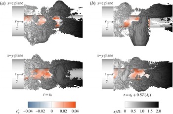
Visualization of the three-dimensional shape of the antisymmetric modes at
 $Sr_{D}\approx 0.2$
using pressure iso-surface in side and top views, i.e.
 $x$
–
 $z$
and
 $x$
–
 $y$
planes, colour coded by the streamwise coordinate
 $x/D$
. The nozzle wall is colour coded by the pressure coefficient increment
 $c_{p}^{\prime }$
.

The shown results already indicate that the antisymmetric modes have a longitudinal plane of symmetry which is randomly oriented in the azimuthal direction and depends on the choice of the considered time segment. Nevertheless, the true three-dimensional shape of the antisymmetric mode responsible for periodic buffet loads at
 $Sr_{D}\approx 0.2$
needs additional clarification due to the existing controversy of the widely spread assumption of an underlying helical structure discussed in § 3.2.2. Since standard vortex identification methods such as vorticity contours, iso-surfaces of Q-criterion or
 $\unicode[STIX]{x1D706}_{2}$
on a reduced-order velocity field do not yield a unique result due to overprinting of the coherent large-scale motion by smaller turbulent structures, the relation between the pressure and velocity modes is considered. It is known that in shear layer flows, the pressure minima coincide with the vortex centres, while the pressure maxima coincide with the position of stagnation points between the vortices (e.g. Lele Reference Lele1988). Figure 19 shows the iso-surface of the negative pressure fluctuation in the reduced-order modelled flow field at
 $Sr_{D}\approx 0.2$
in side and top view, i.e. planes
 $x$
–
 $z$
and
 $x$
–
 $y$
. Figure 19(a,b) show two time instances separated by one half of the vortex shedding period. The temporal evolution clearly indicates an antisymmetric formation of inclined closed-loop vortices which convect downstream and undergo a strong elongation in the streamwise direction once they leave the recirculation area and interact with the free stream. Again, for a more dynamic impression, the reader should view the supplementary movie which is available online. Thus, in contrast to the widely spread assumption, the antisymmetric mode, which is responsible for periodic side loads at the frequency
 $Sr_{D}\approx 0.2$
in the transonic wake of an Ariane 5-like configuration, has a shape of inclined elongated closed-loop vortices. These are shed antisymmetrically from the opposite azimuthal positions which span a momentarily longitudinal plane of symmetry that temporarily changes its orientation randomly, resulting in an axisymmetric time-averaged field and spatially isotropic buffet loads.
4 Summary and conclusions
A reduced-order analysis based on optimized dynamic mode decomposition has been performed on the turbulent wake of a generic Ariane 5-like configuration at transonic free stream conditions (
 $Ma_{\infty }=0.8$
and
 $Re_{D}=6\times 10^{5}$
). The three-dimensional high-fidelity input data have been computed using a zonal RANS–LES method in conjunction with synthetic turbulence generation and validated by experimental results. The analysed flow topology is characterized by an unsteady recirculation region formed around the nozzle due to the separation of the incoming turbulent boundary layer at the main body shoulder and subsequent reattachment of the developed shear layer onto the nozzle surface, which results in strongly periodic wall pressure fluctuations.
Using conventional statistical analysis, three characteristic frequency ranges, i.e.
 $Sr_{D}\approx 0.1$
,
 $Sr_{D}\approx 0.2$
and
 $Sr_{D}\approx 0.35$
have been identified in the wall pressure fluctuations. Furthermore, despite the axisymmetric geometry and zero angle of attack, footprints of non-axisymmetric modes and resulting side forces, known as the buffet phenomenon, have been detected which feature energetically most pronounced fluctuations at
 $Sr_{D}\approx 0.2$
followed by distinct, but energetically less strong peaks at
 $Sr_{D}\approx 0.35$
.
Subsequent analysis of the reduced-order modelled flow field based on the extracted DMD modes shows that the first distinct frequency range,
 $Sr_{D}\approx 0.1$
, is associated with a longitudinal cross-pumping motion of the separation bubble caused by a harmonic antisymmetric oscillation of the main recirculation vortex in the streamwise direction. For the second range,
 $Sr_{D}\approx 0.2$
, a cross-flapping motion of the shear layer is determined. It is triggered by antisymmetric vortex shedding which is in phase with the cross-pumping motion and therefore, features a doubled frequency value. The third frequency range,
 $Sr_{D}\approx 0.35$
, is attributed to a swinging motion of the shear layer caused by a higher harmonics of the vortex shedding mode.
Finally, the three-dimensional shape of the energetically most relevant antisymmetric mode at
 $Sr_{D}\approx 0.2$
, mainly associated with the buffet phenomenon, is scrutinized and in contrast to the widely spread assumption in the literature, no periodic helical motion is detected. Instead, inclined elongated closed-loop vortices are identified that are shed in alternating sequence from azimuthally opposite positions in a momentarily longitudinal plane of symmetry that changes its orientation from time to time randomly, maintaining an axisymmetric time-averaged field and spatially isotropic buffet loads.
Acknowledgements
Financial support from the German Research Foundation (Deutsche Forschungsgemeinschaft DFG) in the framework of the Sonderforschungsbereich Transregio 40 is gratefully acknowledged by the authors. The authors would also like to acknowledge Professor P. Schmid and Professor T. Sayadi for valuable discussions and shared knowledge on modal decomposition methods within the framework of the Transregio 40 Summer Research Program. Computational resources have been provided by the Stuttgart High-Performance Computing Center (Höchstleistungsrechenzentrum Stuttgart, HLRS).
Supplementary movies
Supplementary movies are available at https://doi.org/10.1017/jfm.2017.46.