





1. Introduction
The development of scramjet combustors remains fundamentally constrained by the complex interplay between shock-dominated flows and finite-rate chemistry. While pioneering theoretical frameworks by Ferri (Ferri et al. Reference Ferri, Libby and Zakkay1964; Ferri & Fox Reference Ferri and Fox1969) and Billig (Billig Reference Billig1967; Billig & Dugger Reference Billig and Dugger1969; Billig Reference Billig1988) established the first comprehensive design methodologies for supersonic combustion systems, their analytical approaches necessarily simplified the full three-dimensional (3-D) physics of turbulent reacting flows. These foundational works addressed key aspects of shock–flame interactions and compressible mixing layers, but could not fully account for the vorticity generation mechanisms and transverse instability modes observed in actual engine flows. The persistent challenge of unstart highlights this gap between theoretical prediction and experimental observation. Remarkably, despite six decades of research building on these classical works, along with modern computational studies (Genova et al. Reference Genova, Otero, Stiehl, Reyes, Martin and Ahmed2019; Lee & Lee Reference Lee and Lee2024; Araújo et al. Reference Araújo, Bezerra, Souza and Toro2024), no full-scale scramjet has achieved sustained operational viability.
The transverse jet in supersonic crossflow (JISCF) has emerged as a canonical configuration for investigating supersonic combustion physics, as it encapsulates the key fluid dynamic phenomena present in practical scramjet combustors. As demonstrated by Gamba et al. (Reference Gamba, Miller, Mungal and Hanson2011), this configuration preserves the essential features of shock–boundary layer interactions (SBLIs), compressible shear-layer development and large-scale turbulent mixing while generating the recirculation zones critical for flame stabilisation. Its geometric simplicity renders it uniquely amenable to detailed experimental characterisation and high-fidelity numerical simulation, bridging the gap between fundamental research and applied combustor design. The configuration’s scientific utility is evidenced by its adoption across multiple research programmes, from fundamental studies of jet-crossflow dynamics (Karagozian Reference Karagozian2010; Huang & Yan Reference Huang and Yan2013; Huang Reference Huang2016) to applied investigations of operational systems, including the HyShot II scramjet (Hass et al. Reference Hass, Smart and Paull2005; Smart et al. Reference Smart, Hass and Paull2006) and laboratory-scale combustors (Gamba et al. Reference Gamba, Miller, Mungal and Hanson2011, Reference Gamba, Miller, Mungal and Hanson2012; Gamba & Mungal Reference Gamba and Mungal2015).
The JISCF configuration has been extensively studied through both computational (Liang et al. Reference Liang, Sun, Liu and Yang2018; Rasheed & Mishra Reference Rasheed and Mishra2023; Sharma et al. Reference Sharma, Singh, Angelilli and Raman2024b) and experimental (Gamba & Mungal Reference Gamba and Mungal2015; Gevorkyan et al. Reference Gevorkyan, Shoji, Getsinger, Smith and Karagozian2016; Liu et al. Reference Liu, Sun, Liang, Cai and Wang2018; Nilsson et al. Reference Nilsson, Zhong and Fureby2021) approaches, with parallel investigations of confined configurations (Sun & Hu Reference Sun and Hu2018; Zhao et al. Reference Zhao, Du, Yang, Tang and Sun2022; Xiong et al. Reference Xiong, Sun, Yu, Hu, Yang, Wang and Wang2022). While these studies have significantly advanced understanding of geometric effects on flow topology (Xiong et al. Reference Xiong, Sun, Yu, Hu, Yang, Wang and Wang2022), mixing (Smith & Mungal Reference Smith and Mungal1998) and flame anchoring mechanisms, critical gaps remain in characterising shock-mediated choking phenomena. Notably absent is systematic examination of how SBLIs modulate the transition to thermal choking – a pivotal process governing scramjet unstart thresholds. This oversight persists despite theoretical recognition of choking’s importance, as evidenced by the comparative analysis of Larsson et al. (Reference Larsson, Laurence, Bermejo-Moreno, Bodart, Karl and Vicquelin2015) of Fanno–Rayleigh flow predictions for unchoked conditions. Their work demonstrated the limitations of classical one-dimensional (1-D) theory in capturing near-wall phenomena, particularly the dramatic pressure rise coupled with wall heat losses, yet stopped short of exploring choked flow regimes. To align with 1-D theory, their model required the inclusion of wall heat losses.
The current paradigm in scramjet design criteria (Lee & Lee Reference Lee and Lee2024; Araújo et al. Reference Araújo, Bezerra, Souza and Toro2024) remains disproportionately focused on heat addition effects while under-representing the coupled thermo-compressive dynamics of shock-induced choking. Where Larsson et al. (Reference Larsson, Laurence, Bermejo-Moreno, Bodart, Karl and Vicquelin2015) provided foundational insights into wall-bounded flow physics for unchoked systems, their framework requires extension to address: (i) 3-D shock-train formation under confinement, (ii) viscous–inviscid interactions during choking onset and (iii) the spectral signature of flow transitions. Such advancement would bridge the existing disconnect between theoretical models of compressible duct flow and observed scramjet operability limits, particularly for configurations employing transverse fuel injection – where the JISCF literature has catalogued complex features like horseshoe vortices and shear-layer instabilities (Karagozian Reference Karagozian2010; Huang Reference Huang2016) without quantifying their role in choking dynamics.
The flow structure induced by transverse injection in both supersonic and subsonic crossflows has remained a focal point of fundamental compressible flow research, with spectral analysis emerging as a powerful tool for characterising coherent structures. Seminal work by Fric & Roshko (Reference Fric and Roshko1994) established hydrodynamic analogies between jet plumes and cylindrical bluff bodies, identifying periodic wall signatures that validate the existence of counter-rotating vortex pairs (CVPs) through spectral decomposition. This approach has been extended to more complex geometries, as demonstrated by Ramachandra et al. (Reference Ramachandra, Bhardwaj, Murugan and Sriram2023), who employed spectral methods to quantify distinct modal structures generated by shock train downstream of square-faced protuberances. Their findings revealed that lower-frequency modes reflect large-scale separation dynamics and shock structures. Such analyses provide a template for examining choking precursors in confined scramjet flows, where analogous modal transitions may signal impending thermal choking.
Thermal choking in confined supersonic flows initiates a self-sustaining cycle of unsteady phenomena. The abrupt flow deceleration generates oscillating backpressure that propagates upstream through shockwave dynamics (Su et al. Reference Su, Ji and Chen2016). This destabilises the shock-train structure, leading to large-amplitude oscillations that modulate the entire flow field. The coupling between shock motion, boundary-layer separation and thermal energy release creates a feedback loop where each process amplifies the others. Downstream of the choking point, the flow exhibits heightened unsteadiness in all key variables, with fluctuations becoming increasingly coherent as the system approaches global instability. The choked flow dynamics is governed by a coupled interaction between acoustic waves and vortical structures, both generated by flow separation and downstream pressure recovery mechanisms (Hunt & Gamba Reference Hunt and Gamba2019). The onset of flow choking induced self-sustained oscillations in the shock-train structure, as the system continuously adjusted to match the time-varying backpressure conditions through upstream Mach number modulation (Xiong et al. Reference Xiong, Fan, Wang and Tao2018). The shock system associated with unstart propagated to a more downstream position when triggered by mass addition compared with mechanical blockage scenarios. This displacement reflects fundamental differences in the transient pressure wave propagation characteristics between thermal and geometric flow obstruction mechanisms (Im et al. Reference Im, Baccarella, McGann, Liu, Wermer and Do2016).
Active flow control strategies have further illuminated the connection between separation and choking susceptibility. Recent experiments by Chandravamsi et al. (Reference Chandravamsi, Bhardwaj, Ramachandra and Sriram2023) demonstrated that suppressing bow-shock-induced separation via pulsed actuation increases the effective channel area, as the maximum separation suppression reported in their study was 16.5
 $\,\%$
. However, no study has yet correlated specific spectral signatures with quantitative choking thresholds. Bridging this gap requires coupled spectral–energetic analyses of the type pioneered in bluff-body studies (Fric & Roshko Reference Fric and Roshko1994), but adapted for confined, reacting transverse jet flows where compressibility effects dominate.
This study investigates shock-dominated choking phenomena in confined supersonic flows through a combined theoretical and computational framework. Section 2 presents the governing equations for compressible reacting flow, followed by detailed computational methodology in § 3. Section 4 establishes the classical 1-D Rayleigh flow theory as a baseline for choking analysis. To isolate 3-D effects, systematic comparisons are made between (i) a simplified controlled computational two-dimensional (2-D) configuration that eliminates boundary-layer noise on the upper wall of the combustor while maintaining the no-slip condition on the lower wall to keep a communication pathway (Xiong et al. Reference Xiong, Fan, Wang and Tao2018) and clearly reveal the structure of the emergent low-frequency global mode, and (ii) a full 3-D simulation capturing all flow features which validates the mode’s physical existence and provides a core comparison that reveals the limitations of Rayleigh flow theory. Section 6 quantitatively contrasts the 1-D theoretical predictions with 3-D simulation results, revealing the critical role of multi-dimensional shock dynamics. A novel choking criterion, supported by probe-based spectral analysis of the shock-train region and the dynamic mode decomposition (DMD) of the identified mode, is proposed in § 7, identifying distinct frequency signatures associated with the established choked state. The study culminates in a revised choking paradigm, presented in § 8, which establishes the emergence of a global mode as the diagnostic precursor to flow collapse, with direct consequences for predicting scramjet unstart.
2. Governing equations
A multi-step method is used to calculate the heat release or absorption due to chemical reactions. The chemical reaction kinetics model used in this study is the
 $\text{H}_2$
–air FFCM-1 reaction mechanism proposed by Smith et al. (Reference Smith, Tao and Wang2016). CHEMKIN is used to define the chemical reactions for the current combustion system. The mechanism includes eleven species (
 $\text{H}, \text{H}_2, \text{O}, \text{O}_2, \text{OH}, \text{H}_2\text{O}, \text{HO}_2, \text{H}_2\text{O}_2, \text{O}_3, \text{AR}, \text{N}_2$
). In this study, species containing carbon or helium were excluded, reducing the reversible chemical reactions to 27 equations. This simplification maintains the accuracy of the
 $\text{H}_2$
–air combustion while improving the computational efficiency.
The compressible reactive Navier–Stokes equations are solved using Eulerian uniform grid (Poludnenko & Oran Reference Poludnenko and Oran2010). The continuity, momentum, energy and chemical species equations can be written as the following:
 \begin{equation} \partial _t \rho +\boldsymbol{\nabla }\boldsymbol{\cdot }(\rho u)=0 ,\end{equation}
 \begin{equation} \partial _t (\rho u) +\boldsymbol{\nabla }\boldsymbol{\cdot }(\rho u\otimes u)= -\boldsymbol{\nabla }\!p+\boldsymbol{\nabla }\boldsymbol{\cdot }\tau ,\end{equation}
 \begin{equation} \partial _t (E) +\boldsymbol{\nabla }\boldsymbol{\cdot }((E+p)u)= -\boldsymbol{\nabla }\boldsymbol{\cdot }(-(u\boldsymbol{\cdot }\tau )+q) +\rho q \dot {\omega }, \end{equation}
 \begin{equation} \partial _t (\rho Y_k) +\boldsymbol{\nabla }\boldsymbol{\cdot }(\rho Y_k u)= \rho \dot {\omega _k}-\boldsymbol{\nabla }\boldsymbol{\cdot }j_k ,\end{equation}
where
 $\rho$
is the density, u is the velocity,
 $\tau$
is the stress tensor, E is the energy density, q is the heat flux,
 $\dot {\omega }$
is the reaction rate,
 $Y_k$
is the mass fraction of the specie and
 $j_k$
accounts for any diffusive process (including the Brownian diffusivity, thermal diffusivity and the intermolecular forces).
The equation of state implemented in the code (chemical equation of state) is a multi-species, thermally perfect gas model based on NASA polynomial fits, designed for reactive flow simulations with temperature-dependent thermodynamic properties. The procedure begins by reading species-specific thermodynamic data from CHEMKIN-format input files (e.g. chem.inp and therm.dat), which provide seven-coefficient NASA polynomials for each species in two temperature ranges (low and high). The equation of state calculates pressure using the ideal gas law:
 \begin{equation} p=\rho \textit{RT}/\bar {W} ,\end{equation}
where
 $\bar {W}$
is the mixture-averaged molecular weight derived from species mass fractions (
 $Y_i$
) and individual molecular weights (
 $W_i$
).
Internal energy is computed as a mass-weighted sum of species energies:
 \begin{equation} e=\sum _i Y_i e_i(T) ,\end{equation}
where
 $e_i(T)$
is obtained by integrating the species-specific heat capacity (
 $C_{v,i}$
) derived from the NASA polynomials. Temperature is determined iteratively via Newton–Raphson to satisfy energy conservation, while thermodynamic properties such as heat capacities (
 $C_{\!p}, C_v$
) and the adiabatic index (
 $\gamma$
) are evaluated using polynomial fits.
The implementation also includes energy relaxation to stabilise numerical solutions by separating thermal and non-thermal energy components. This approach ensures accurate modelling of chemically reacting flows with rigorous treatment of temperature-dependent species properties and mixture rules.
The simulations employ dynamic patch-based adaptive mesh refinement (AMR) on a uniform base grid using Athena-RFX++ (Stone et al. Reference Stone, Gardiner, Teuben, Hawley and Simon2008, Reference Stone, Mullen, Fielding, Grete, Guo, Kempski, Most, White and Wong2024; White et al. Reference White, Stone and Gammie2016). Refinement criteria are based on gradients of pressure and OH concentrations. After the initial transient, the AMR refines essentially the entire domain to the highest refinement level, yielding a uniformly spaced effective grid of
 $\approx$
87
 ${\unicode[Arial]{x03BC}}\mathrm{m}$
throughout the channel, injector plume, shock train and flame region. The first cell centre is located approximately 44
 ${\unicode[Arial]{x03BC}}\mathrm{m}$
from the wall, producing averaged
 $y^+\approx 10$
. For reference, a direct numerical simulation (DNS) resolution of
 $y^+ \approx 1$
would require a first cell size of 5–10
 ${\unicode[Arial]{x03BC}}\mathrm{m}$
in this flow, varying with streamwise location, which was computationally prohibitive for the present domain. The present resolution therefore defines a high-fidelity quasi-DNS (QDNS) that far exceeds typical resolutions in the literature for similar domains (Fiévet et al. Reference Fiévet, Voelkel, Koo, Raman and Varghese2017; Larsson et al. Reference Larsson, Laurence, Bermejo-Moreno, Bodart, Karl and Vicquelin2015; Rising et al. Reference Rising, Ching and Johnson2026), ensuring accurate capture of SBLIs, separation dynamics and the low-frequency global mode.
The simulations employ a fully unsplit corner-transport upwind (CTU) scheme coupled with an HLLC Riemann solver (Toro Reference Toro2013). The CTU scheme was selected for its superior accuracy in capturing multi-dimensional wave interactions – a critical feature for resolving complex flow dynamics in Athena-RFX++ (Stone et al. Reference Stone, Tomida, White and Felker2020). By avoiding dimensional splitting, the unsplit CTU approach preserves cross-dimensional flux coupling, ensuring robust treatment of shocks and discontinuities while maintaining high-order spatial accuracy.
The Athena-RFX solver has been widely adopted in turbulent combustion research, with numerous studies validating its numerical framework and convergence behaviour (Poludnenko & Oran Reference Poludnenko and Oran2010; Poludnenko et al. Reference Poludnenko, Gardiner and Oran2011, Reference Poludnenko, Chambers, Ahmed, Gamezo and Taylor2019; Jozefik et al. Reference Jozefik, Harvazinski, Sankaran, Dammati, Poludnenko, Lu, Kerstein, Xu and Wang2024). Collectively, these studies establish Athena-RFX as a benchmark tool for high-fidelity combustion simulations, leveraging its well-documented numerical stability and predictive accuracy.
3. Computational model
The simulation employs a square channel with a 4.5 cm height to model a sonic jet interacting with a supersonic crossflow, as illustrated in figure 1. The domain is strategically partitioned into three distinct regions, following the validated approach of Sun & Hu (Reference Sun and Hu2018) and Xiong et al. (Reference Xiong, Sun, Yu, Hu, Yang, Wang and Wang2022), to isolate key physical processes and optimise computational efficiency.
Schematic of the computational domain for the JISCF, showing the upstream boundary-layer (BL) development region, the jet injection location and the downstream domain with adaptive mesh refinement.

The upstream section is dedicated to developing the boundary layer naturally, ensuring the theoretical transition takes place at the injector. To prevent numerical artefacts, the inlet edges initially implement slip wall boundary conditions (Rising et al. Reference Rising, Ching and Johnson2026). This transitions downstream to physical no-slip conditions, allowing the boundary layer to develop naturally before encountering the jet injection site. This staged approach maintains flow fidelity while minimising spurious oscillations.
At the designated injection point, AMR dynamically concentrates grid resolution to capture critical flow features. The AMR criteria target vortical structures, shock-induced pressure gradients and combustion zones identified by OH radical concentrations, aligning with the high-fidelity methodology of Sharma et al. (Reference Sharma, Bielawski, Rauch and Raman2024a ). This localised refinement ensures accurate resolution of the jet shear-layer dynamics and shock interactions without excessive computational cost.
The downstream section extends sufficiently far to dissipate reflected waves and prevent upstream contamination. To balance accuracy and efficiency, mesh resolution is progressively reduced in this region. The reactions are turned off (non-reacting zone). Slip boundary conditions are reapplied on channel walls to eliminate artificial shock formation that could arise from abrupt mesh coarsening. This design choice preserves solution stability while minimising domain size requirements.
The three-zone structure bridges experimental realism and computational tractability. The boundary-layer zone establishes a physically meaningful inflow, the refined region resolves multi-scale jet–crossflow interactions and the coarsened non-reacting outflow ensures practical simulation runtimes. This set-up has been benchmarked against experimental data to confirm its ability to capture essential flow physics while maintaining numerical robustness. The methodology provides a framework for systematic analysis of mixing, combustion and shock dynamics in supersonic flows, while maintaining adiabatic wall conditions to isolate the thermal effects of the jet–crossflow interaction. Furthermore, the present computational framework reproduces the lower-wall separation angle associated with the V-shaped collision-shock structure downstream of the injector, in close agreement with reported measurements, and it is provided in Appendix A.
4. Rayleigh flow
Effect of different HRR profiles (uniform, linearly increasing, linearly decreasing) on flow choking in 1-D Rayleigh flow. The plot shows the Mach number and the HRR distributions along the duct, illustrating the formation and upstream propagation of a normal shock under supercritical heat addition (
 $q \gt q^*$
). All profiles, with identical total heat addition, lead to the same choked exit condition.

Numerical investigations were conducted to examine three distinct heat release rate (HRR) profiles under supercritical (
 $q\gt q^*$
) conditions in a 1-D supersonic flow with a Mach number M = 3.2, static temperature T = 1400 K and static pressure P = 0.75 bar. The critical heat release rate was determined to be
 $q^* =3.62838\times 10 ^{10}\ \text{erg cm}^{-3} \ \text{s}^{-1}$
. As illustrated in figure 2, the study considered (i) a uniform HRR profile, (ii) a linearly increasing profile and (iii) a linearly decreasing profile, enabling a systematic comparison of their effects on flow dynamics.
Heat addition was confined to a constant-area channel between axial positions X = 30 cm and X = 60 cm, ensuring isolation of pure Rayleigh flow effects. To facilitate a meaningful comparison, the total integrated heat addition (i.e. the area under the HRR curve) was maintained identical across all profiles. The linear profiles were designed such that
 \begin{equation} \int _{30}^{60} q_{\textit{linear}}(x) \, \text{d}x = \int _{30}^{60} q_{\textit{constant}} \, \text{d}x, \end{equation}
ensuring equivalent total energy input while allowing examination of profile-dependent thermodynamic responses.
To extend the analysis beyond critically choked flow, supercritical conditions (
 $q\gt q^*$
) were investigated. Adopting the same numerical methodology as in the critical cases, three distinct HRR profiles – each exceeding the previously determined critical threshold (
 $q^*=3.62838\times 10^{10}\,\text{erg cm}^{-3}\text{s}^{-1}$
) – were examined under identical inflow conditions (M = 3.2, T = 1400 K, P = 0.75 bar). This approach maintains consistency with the baseline study while elucidating the thermodynamic and flow responses to supercritical heat addition, particularly in terms of thermal choking and downstream evolution.
Figure 2 demonstrates the formation and upstream propagation of a normal shockwave in response to supercritical heat addition (
 $q \gt q^*$
), representing a fundamental adjustment mechanism in supersonic flows. The shockwave induces a discontinuous transition to a new Rayleigh line characterised by reduced specific mass velocity (G), effectively modifying the flow’s thermodynamic pathway.
For all three HRR profiles examined, the shockwave systematically decelerated the flow to subsonic conditions. Subsequent heat addition then reaccelerated the flow, culminating in sonic conditions (M = 1) at the duct exit. This persistent choking at the downstream boundary, observed across all supercritical cases, demonstrates the robustness of thermal choking as a governing constraint. The shock-mediated adjustment process particularly underscores the dominant role of compressibility in maintaining mass conservation under varying thermal energy deposition.
These findings are in excellent agreement with theoretical predictions for Rayleigh flow: when excessive heat addition occurs, the flow must undergo a shock transition to subsonic conditions before thermal re-acceleration can re-establish choking at the exit. This self-consistent adjustment mechanism simultaneously accommodates the imposed energy input while preserving the critical choking condition, thereby ensuring global conservation of mass and momentum.
Figure 2 reveals distinct flow responses to different HRR profiles under supercritical conditions. The decreasing HRR profile produces a significant Mach number recovery downstream of the shockwave, while the increasing profile primarily modifies flow conditions near the heat addition termination point. Notably, all profiles converge to identical final thermodynamic states, demonstrating that the critical choking condition remains the governing constraint.
These results highlight an important dichotomy in Rayleigh flow dynamics: while the spatial distribution of heat addition significantly influences intermediate flow features – including local Mach number variations and pressure gradient development – the terminal state remains uniquely determined by the choking condition. This invariance of the final state with respect to HRR profiles underscores the primacy of global conservation laws in establishing the exit conditions. The flow consistently achieves sonic velocity at the downstream boundary, independent of the specific thermal deposition history, confirming that integral constraints dominate over local heating details in determining the asymptotic solution.
The P–v diagrams presented in figure 3 elucidate the thermodynamic evolution of the flow following shockwave formation. The supersonic inflow initially adheres to the original Rayleigh line (blue solid curve) until encountering the shock discontinuity, which abruptly transitions the flow to the subsonic branch via the shock adiabat. This transition is accompanied by a marked increase in static pressure and temperature, a reduction in mass velocity (G) and an irreversible increase in entropy.
Pressure–specific volume (P–v) diagram for supercritical Rayleigh flow with a shock transition. The trajectory shows the supersonic inflow on the Rayleigh line (blue solid line), the jump to the subsonic branch via the shock adiabat (red dashed-dot line) and the subsequent evolution to the unique sonic (M = 1) exit condition at the intersection with the product adiabat (black dotted line).

A key observation is the unique intersection between the post-shock Rayleigh line and the product adiabat, which precisely corresponds to sonic conditions (M = 1) at the duct exit. This singular solution highlights the deterministic nature of thermally choked flows: despite the shock-induced modification of static properties, the system invariably evolves towards a choked state. The invariance of this terminal condition reinforces that the exit Mach number is fundamentally constrained by global conservation laws rather than transient adjustment processes.
These results demonstrate that the shockwave serves as a critical mediator, reconciling excessive heat addition with mass conservation requirements. By bridging the supersonic and subsonic regimes, the shock adiabat enables the flow to satisfy both energy and momentum constraints while preserving the choking criterion. This behaviour is fully consistent with Rayleigh flow theory, wherein the cumulative heat input exclusively determines the final state, independent of the specific heat release profile. The P–v trajectories thus confirm that the shock-mediated transition represents a necessary thermodynamic pathway to achieve choked exit conditions under supercritical heating.
However, the local progression of flow properties exhibits pronounced profile dependence. The decreasing HRR profile induces rapid pressure and temperature increases near the heating zone entrance, while the increasing profile delays these changes until the downstream region. This differential response suggests that HRR profiling can serve as an effective flow control mechanism. Front-loaded distributions may be employed to promote early thermal choking, whereas rear-loaded profiles could strategically delay property variations for applications requiring extended supersonic regions.
These findings highlight an important design consideration: while global constraints dictate the final state, local heat release modulation offers a means to tailor transient flow behaviour without altering the terminal conditions. Such controllability could prove valuable for optimising scramjet combustors or other high-speed flow systems where precise management of shock formation, jet injections and thermal gradients is critical. However, this is beyond the scope of the paper.
5. Two-dimensional and three-dimensional choking
5.1. Two-dimensional flow conditions
Table 1 summarises the flow conditions for a choked 2-D case with
 $J=1.17$
(slightly above the critical threshold). These conditions will later be compared with 3-D simulations to quantify the dimensional effects on choking. Despite their limitations, the 2-D results enhance the intuition about the underlying physics, such as SBLIs and blockage effects, which remain relevant in 3-D flows.
The flow conditions of the two-dimensional jet in supersonic crossflow simulation.

Table 1. Long description
The table has two rows of data and three columns: temperature in kelvin, static pressure in bar, and Mach number. The crossflow row gives a temperature of 1400 kelvin, a static pressure of 0.75 bar and a Mach number of 3.2. The jet row gives a temperature of 300 kelvin, a static pressure of 9 bar and a Mach number of 1.
The 2-D channel configuration, adapted from the 3-D computational framework (§ 3), exhibited choking at significantly lower momentum flux ratios (J) than its 3-D counterpart. Key modifications included: (i) extending the slip-wall condition to x = 7 cm to suppress boundary-layer development, (ii) positioning the injector at x = 8 cm for flow stabilisation and (iii) applying AMR prior to x = 72 cm with an upper slip wall to isolate inviscid shock dynamics. These adjustments eliminated 3-D effects – turbulent mixing, sidewall vortices and boundary-layer separation – thereby reducing momentum losses and advancing the choking onset. The 1152 cm domain length ensured outflow boundary independence, while the slip condition simplified the flow topology, yielding coherent Mach stems and unambiguous choking signatures.
The observed leftward shift in the choking threshold underscores the dominant role of dimensionality in compressible flow resistance. In two dimensions, the absence of spanwise dissipation pathways allows shock trains to stabilise with weaker adverse pressure gradients, explaining the reduced J requirement. The AMR-resolved flow fields confirmed quasi-steady shock structures, validating the numerical framework’s ability to capture inviscid choking criteria without 3-D artefacts. While this simplification clarifies fundamental mechanisms – such as the direct correlation between choking and bulk flow deceleration – it also highlights the necessity of reintroducing 3-D effects for practical systems, where turbulent mixing and boundary-layer interactions critically modulate the choking limit.
The flow evolution was systematically analysed through temporal snapshots at five characteristic instants, with pressure contours depicted in figure 4. The simulations reveal that Mach stem formation commenced immediately upon initialisation (figure 4 a), indicating rapid establishment of choking conditions. Subsequent temporal evolution demonstrated progressive downstream pressure accumulation (figure 4 a–c), which ultimately generated upstream-propagating disturbances culminating in unstart initiation. This process manifested through two distinct yet coupled phenomena: (i) the formation of a normal shockwave upstream of the injector and (ii) the temporal development and upstream migration of the downstream-originating shock structure.
Temporal evolution of pressure contours (in barye) illustrating the choking process in the 2-D JISCF configuration. Snapshots at (a) t = 0.3 ms, (b) t = 0.7 ms, (c) t = 1.59 ms, (d) t = 2.389 ms and (e) t = 3.3 ms show the formation of the Mach stem, downstream pressure accumulation and the upstream propagation of disturbances leading to unstart. The locations of pressure probes used for spectral analysis are indicated.

The observed dynamics highlights a critical feedback mechanism wherein downstream pressure buildup drives upstream shock formation, which in turn amplifies Mach stem growth. This mutual reinforcement between downstream and upstream wave systems ultimately leads to complete flowpath unstart. The time-resolved visualisation provides clear evidence of the shock interactions that characterise this transitional process, with particular emphasis on the spatial progression of wavefronts and their role in establishing the final unstart configuration.
In short, the 2-D configuration serves as a controlled numerical experiment to isolate the inviscid core of the global mode. Slip conditions on the upper wall are applied to: (i) eliminate boundary-layer disturbances that could mask system-scale dynamics, (ii) suppress upstream acoustic propagation through the upper wall while maintaining an upstream communication pathway through the no-slip lower wall (a separate supersonic confinement effect) and (iii) verify that the mode originates from bulk shock–flow interaction, not from random wall-generated turbulence. This approach clarifies the fundamental wave feedback responsible for choking.
The flow conditions of the three-dimensional jet in supersonic crossflow simulations at varying momentum flux ratios (J).

Table 2. Long description
The table has two rows of data and three columns: temperature in kelvin, static pressure in bar, and Mach number. The crossflow row gives a temperature of 1400 kelvin, a static pressure of 0.75 bar and a Mach number of 2.7. The jet row gives a temperature of 300 kelvin and a Mach number of 1, with three static pressures of 7.6659, 15.33 and 30 bar. These correspond to momentum flux ratios of 1.5, 3.0 and 5.87 respectively.
5.2. Three-dimensional flow conditions
The 3-D refined computational domain extends from x = 0 to 40 cm. Table 2 summarizes the flow conditions for the 3-D cases. A brief slip-wall region (
 $x\lt 2$
cm) is applied at the inlet to prevent spurious numerical reflections (Rising et al. Reference Rising, Ching and Johnson2026), after which no-slip boundary conditions are enforced on all walls to allow natural boundary-layer development. The injector, with a radius of 1.6 mm, is positioned at x = 8.4 cm, providing a development length of
 $\approx 6.3$
cm from the start of the no-slip region. Over this distance, the local theoretical Reynolds number based on streamwise distance from the effective origin reaches
 $Re_x\approx 4.7\times 10^5$
– a value that lies within the natural transitional range for a flat-plate boundary layer. No artificial tripping is employed; the inflow profile develops self-consistently from the governing equations under the specified boundary conditions. This approach avoids introducing arbitrary trip parameters and ensures the inflow is determined solely by the governing equations and specified boundary conditions. The flow was initialised to the inflow conditions.
To ensure accurate flame and shear-layer resolution, this work adopts the experimental observations of Gamba & Mungal (Reference Gamba and Mungal2015), who report an average OH layer thickness of 0.3 mm – a scale which is associated with the shear-layer thickness in the simulations. This follows the resolution criteria established by Attili et al. (Reference Attili, Bisetti, Mueller and Pitsch2014), which prescribe 3–10 grid points across the shear layer. This resolution guarantees proper capture of both the flame structure and mixing dynamics, while remaining computationally tractable for the domain size under consideration.
To assess the choking behaviour across different momentum flux ratios (J), pressure iso-surfaces were analysed at 1.5 ms to identify the onset of flow obstruction. Figure 5 illustrates the pressure distribution using three distinct iso-surfaces (1, 3 and 5 bar). For J = 1.5, the flow remains largely unperturbed, with pressure levels consistently near 1 bar throughout the domain (figure 5 a). In contrast, at J = 3, a moderate pressure rise is observed downstream, particularly along the lower wall, though the peak pressure remains below 3 bar. This suggests increased flow resistance but not yet sufficient to induce full choking.
Instantaneous pressure iso-surfaces (1, 3 and 5 bar) in the 3-D JISCF at t = 1.5 ms for momentum flux ratios (a) J = 1.5, (b) J = 3.0 and (c) J = 5.87. The onset of significant flow blockage and high-pressure regions downstream signals the transition to choking at J = 5.87.

The most pronounced effects are seen at J = 5.87, where a clear pressure buildup emerges downstream, with the 3 bar iso-surface extending between x = 30 and 40 cm. This localised high-pressure region signals the initiation of choking, as the flow encounters significant blockage due to the jet’s momentum dominance. While the pressure does not reach 5 bar within the observed time frame, the progressive rise with increasing J underscores the role of momentum flux ratio in dictating choking onset. These findings align with theoretical expectations, where higher J values enhance jet penetration and flow restriction, ultimately leading to choking at sufficiently elevated ratios.
The heat release characteristics were quantified through spatial averaging and integration of the volumetric HRR field. Spanwise and wall-normal averaging yielded the local HRR distribution
 $\langle \dot {q} \rangle _{y,z}$
(units:
 $\mathrm{erg\,cm^{-3}\,s^{-1}}$
), while streamwise integration of these profiles provided the total power output
 $\dot {Q}_{total}$
(units:
 $\mathrm{erg\,s^{-1}}$
). This dual approach captures both the local combustion intensity and global energy release, with the integration performed across the entire reaction zone to account for all chemical heat release.
6. Shock-dominated choking: Rayleigh flow versus three-dimensional flow
Building upon the 1-D simulation framework established in § 4, the total HRRs corresponding to J = 1.5, 3.0 and 5.87 (
 $\dot {Q}_{total} = 9.14 \times 10^{10}$
,
 $1.77 \times 10^{11}$
and
 $4.749 \times 10^{11} \, \mathrm{erg\,s^{-1}}$
, respectively) were implemented to examine the system response under supercritical conditions. Consistent with Rayleigh flow theory, the simulations confirmed that the final thermodynamic state remains invariant to the heat release profile, as demonstrated in § 4.
To match the 3-D simulations and theoretical consistency, a uniform heat release profile was adopted between x = 2.1 cm and x = 38.6 cm. This spatial domain was selected to: (i) match the computational configuration and (ii) maintain alignment with classical 1-D Rayleigh flow assumptions, where heat addition occurs across a well-defined control volume. The constant HRR profile serves as a canonical representation for comparing against analytical solutions, while preserving the essential physics of thermally choked flows.
The implementation ensures that the total integrated energy input matches the measured values from the 3-D cases, enabling direct comparison of the 1-D and 3-D results. This approach isolates the role of total heat addition (as opposed to spatial distribution) in determining the terminal flow state, while providing a computationally tractable framework for parametric studies across different injection conditions.
Figure 6 presents a systematic comparison between 1-D Rayleigh flow simulations and spatially averaged 3-D Mach number profiles for three momentum flux ratios (J = 1.5, 3.0, 5.87). In subcritical regimes (J = 1.5 and 3.0), shock-mediated mechanisms – including Fanno flow losses, SBLIs and shock-train formation – collectively account for 10
 $\,\%$
and 16
 $\,\%$
of the total flow deceleration, respectively. This monotonic increase with J reveals a fundamental coupling between momentum flux and shock-driven dissipation: higher J ratios amplify the role of compressibility effects in driving the system towards thermal choking. The results suggest that an effective area reduction model, quantifying the flow constriction induced by shock structures, could improve predictive capabilities for mass flow regulation in confined supersonic ducts.
Comparison of streamwise Mach number distributions from 1-D Rayleigh flow simulations (orange lines) and spatially averaged 3-D results (blue lines) for (a) J = 1.5 (dashed-dot line), (b) J = 3 (dashed line) and (c) J = 5.87 (dotted line). The divergence at J = 5.87, where 3-D simulations choke despite 1-D predictions, highlights the role of multi-dimensional shock dynamics.

The analysis reveals a critical divergence at J = 5.87: while 1-D theory predicts unchoked flow, the 3-D simulations achieve complete choking due to the synergistic action of shock dynamics and wall friction. Here, shock-related mechanisms contribute more towards the deceleration process, contributing over 35
 $\,\%$
of the total momentum loss – a threefold increase relative to the J = 1.5 case. This stark contrast highlights how multi-dimensional effects (particularly SBLI-induced separation, vortical structures and shock-train unsteadiness) fundamentally alter choking thresholds compared with idealised 1-D predictions. This underscores that Rayleigh flow theory, while valuable for establishing baseline behaviour, requires augmentation with shock-loss modelling for accurate predictions in high-J regimes where 3-D effects govern the transition to choked flow.
To quantify the contribution of the shock-based mechanism (including the viscous effects), the contribution was compared with the amount of deceleration needed to decelerate the flow to the sonic speed (M = 1) from the initial state (M = 2.7). The calculations considered the difference between the 1-D Mach number and the 3-D Mach number, as shown in the following equation:
 \begin{equation} \varPi _{\textit{Mechanical}} = \frac {M_{1D}-M_{3D}}{M_{\infty }-M_{\textit{sonic}}}\times 100\,\% ,\end{equation}
where
 $\varPi _{\textit{Mechanical}}$
accounts for the mechanical choking. However, the characteristic length of the choking estimated by Rayleigh flow equations can be used to quantify the choking of the choked case. The estimated characteristic length (
 $L^*_{1D}$
) of the choked case was 45.69 cm, while the shockwave in the choked case started to develop around 32 cm (
 $L^*_{3D}\approx 30$
) with the same amount of volumetric heat release rate. This can indicate that the amount of heat added to the flow to choke in the Rayleigh flow model is much greater than that of the real case.
The characteristic length required for thermal choking was quantified using both a theoretical 1-D Rayleigh flow model and the current 3-D simulation. For a given total heat release, the 1-D model – which is independent of the specific heat release profile – predicts a choking length (
 $L^*_{1D}$
) of 45.69 cm, and it is equivalent to a critical HRR of
 $\dot {Q}_{total} = 5.2572 \times 10^{11} \text{erg}\,\text{s}^{-1}$
. In stark contrast, the 3-D simulation reveals that a shock system, indicative of choking, initiates at a significantly shorter distance of approximately 32 cm (
 $L^*_{3D}\approx 30$
).
In both 1-D and 3-D analyses, thermal choking is identified when the flow Mach number reaches unity. In 1-D Rayleigh flow, this follows directly from the Rayleigh-line relations. In three dimensions, choking is determined by the spatial average of the Mach number profile.
Figure 7 captures the temporal evolution of pressure iso-surfaces for the J = 5.87 case, revealing critical compressible flow dynamics. Upstream of x = 16 cm, the pressure maintains a uniform 1 bar baseline, indicative of the undisturbed supersonic core flow (Mach 2.7). A distinct pressure rise to 3 bar emerges along the lower wall downstream (figure 7 b), coinciding with the heat release zone. This threefold pressure increase at t = 2.5 ms signifies thermal choking, where exothermic reactions reduce the local Mach number to subsonic, triggering a shockwave. Figure 8(a) corroborates this, showing the choked flow’s pressure contour at the same time step, with the shockfront’s position tied to combustion intensity.
Time series of instantaneous pressure iso-surfaces (in barye) for the choked J = 5.87 case at (a) t = 0.7 ms, (b) t = 2.5 ms, (c) t = 3.5 ms and (d) t = 5 ms. The sequence shows the upstream propagation of a high-pressure region and the eventual stabilisation of a normal shock, confirming the establishment of a choked state.

Instantaneous pressure contours (in barye) on the central plane for J = 5.87 at (a) t = 2.5 ms and (b) t = 5 ms. The contours reveal the shockfront position and significant transverse pressure gradients due to 3-D shock–vortex interactions, absent in 1-D models.

The flow evolution exhibits two coupled compressible mechanisms:
-
(i) Upstream shock propagation. The pressure disturbance travels from x = 35 to 16 cm in 2.5 ms, yielding a laboratory-frame speed of 76 m s−1. This slow upstream motion of the shock structure is a hallmark of the choked regime.
-
(ii) Three-dimensional shock–vortex interactions. Corner regions reach 5 bar due to shock reflection and vortical straining (figure 8 a), creating a 2 bar transverse gradient. This asymmetry arises from baroclinic vorticity, which is absent in 1-D models.
By t = 5 ms (figure 7 d), a normal shock stabilises at x = 15 cm, confirming choked flow establishment. The sustained 5 bar (upper wall) versus 3 bar (lower wall) differential underscores the dominance of 3-D effects – particularly boundary-layer separation and vortex–shock coupling – in modifying the choking criterion. This deviation from idealised 1-D Rayleigh flow emphasises the necessity of multi-dimensional analysis for high-J regimes, where shock–turbulence–chemistry interactions govern system behaviour.
7. A shock-driven choking criterion: spectral analysis and mechanical signature
7.1. Spectral signature of choking
The slip boundary condition at the upper wall eliminated boundary-layer vortices, enabling unambiguous identification of pressure fluctuations behind the Mach stem and secondary reflected shock in the 2-D case (figure 9). Power spectra revealed distinct frequency signatures tied to these features: a dominant 305 Hz peak behind the Mach stem, and weaker modes downstream. The low-frequency mode will be studied in the future discussions, while the secondary frequency emerges from some large-scale convective structures or a nonlinear coupling, but it is out of the scope of this study.
Power spectral density (PSD) of pressure perturbations at four streamwise locations (x = [9, 20, 30, 50] cm, and y = 3.9 cm) in the 2-D simulation. The dominant 305 Hz peak is a global feature of the choked flow.

Time-resolved pressure signals were extracted from selected locations along the wall. Due to non-uniform time-step outputs inherent to AMR and Courant–Friedrichs–Lewy-based time stepping, the non-uniform fast Fourier transform (NUFFT) algorithm was employed to compute the spectral content. Each signal consisted of at least 1000 temporally resolved data points spanning a physical window of approximately 3 to 5 ms for the unchoked and the supercritical case.
The NUFFT implementation allows for accurate estimation of spectral components without resampling or interpolation, avoiding spectral distortion or aliasing artefacts associated with uneven sampling. This approach enabled robust identification of dominant low-frequency instabilities associated with shock-induced oscillations and global flow unsteadiness.
The 305 Hz frequency is that of an emergent mode that the entire system locks into. The Mach stem oscillates and contributes energy, but it is a participant in this system-wide resonance, not the sole source of its specific frequency. The elevated energy in the region near the Mach stem confirms its role as a key driver of the instability. The mode itself arises from a balance between large-scale wave propagation and confinement effects that coordinate the entire flow field.
The secondary mode emerges downstream, produced by convective structures as the flow interacts with the walls. This frequency’s appearance coincides with a significant reduction (
 ${\gt} 35\,\%$
) in the primary mode’s amplitude, illustrating an energy cascade from large-scale shock oscillations to finer-scale turbulence. The damping of the 305 Hz signal reflects convective losses, damping of nonlinear waves and vorticity production by Kelvin–Helmholtz instabilities, which disrupt coherent oscillations while enhancing mixing.
The persistence of the primary frequency downstream confirms its connection to global choking dynamics. This dual-scale behaviour aligns with compressible flow theory, where shock-driven instabilities (305 Hz) seed shear-layer vortices, redistributing energy across scales. The spectra collectively quantify how choking-induced oscillations evolve into dissipative structures. The persistence of the dominant mode’s frequency at downstream locations suggests it is a global feature of the flow, rather than a local, spatially dependent instability. In turn, the Lagrangian point can be chosen to be located anywhere downstream of the Mach stem. However, this claim requires further investigations using statistical analysis.
In figure 10(d), the phase angles between four probe locations were analysed to elucidate wave propagation at the dominant mode. The analysis revealed a complex, bidirectional wave structure (table 3). At Probe 3, a phase lead of
 $64^\circ$
relative to Probe 1 was observed, corresponding to a downstream phase speed of 358.2 m s−1 (figure 10
e). This subsonic velocity, characteristic of large-scale convective structures, indicates a mechanism for downstream energy transport from the primary shock system.
Statistical analysis of the 2-D choked flow. (a) Correlation matrix of pressure signals from four probes. (b) Magnitude-squared coherence spectrum. (c) Streamwise velocity phase difference at dominant low-frequency mode. (d) Pressure phase difference at dominant low-frequency mode. (e) Phase speed between probe pairs, revealing bidirectional (downstream convective and upstream acoustic) wave propagation.

Phase angle and phase speed between the four sensors.

Table 3. Long description
The table has six rows, one per probe pair, and four columns: phase speed in metres per second, pressure phase angle, streamwise velocity phase angle, and the difference between the pressure and velocity phase angles. All angles are in degrees. Pair 1 to 2: 148.3, 81.5, 61.7, 19.8. Pair 1 to 3: 358.2, 64.4, 54.0, 10.4. Pair 1 to 4: 1116.6, 40.3, 36.1, 4.2. Pair 2 to 3: negative 642.5, negative 17.1, negative 7.7, negative 9.4. Pair 2 to 4: negative 800.8, negative 41.1, negative 25.6, negative 15.5. Pair 3 to 4: negative 913.2, negative 24.0, negative 17.9, negative 6.2. Positive phase speeds correspond to downstream convective propagation and negative values to upstream acoustic propagation.
At Probe 2, a phase lead of
 $81.5^\circ$
– midstream probes – and nearly half a cycle – was observed relative to Probe 1. The corresponding phase speed of 148.3 m s−1 (figure 10
e) indicates convective communication mediated by large-scale vortical structures. This downstream propagation mechanism is consistent with that identified between Probes 1 and 3.
Conversely, the measured phase lag of
 $-24^\circ$
between Probes 4 and 3 yields a phase speed of −913 m s−1 (figure 10
e), a value that matches the local speed of sound and unambiguously identifies an upstream-travelling acoustic wave. This wave is interpreted as the key component of a feedback loop: it is the acoustic precursor generated by downstream shock oscillations, which travels upstream to trigger new instabilities, completing a cycle that sustains the emergent global mode.
The phase relationships for other probe pairs further reinforced the presence of upstream acoustic feedback. Relative to Probe 2, Probe 3 lagged by
 $-17^\circ$
and Probe 4 by
 $-41.1^\circ$
, yielding upstream phase speeds of −642 and −800.8 m s−1 (figure 10
e), respectively. These negative velocities are a clear signature of slow acoustic communication propagating upstream from the choking zone.
The net communication across the entire domain is captured by the relationship between Probe 4 and Probe 1, where a
 $40.3^\circ$
phase lead and a high phase speed of 1116.4 m s−1 were measured. This value, which aligns with the local speed of sound in the high-temperature sections of the flow, confirms the presence of system-spanning acoustic communication with an average phase speed of −122.2 m s−1 (figure 10
e). This global acoustic wave is responsible for phase-locking the entire flow field, from the upstream Mach stem to the downstream choking zone, on the same dominant low-frequency mode.
To definitively characterise the nature of the observed waves, the phase relationship between the streamwise velocity and pressure fluctuations (
 $\phi _p - \phi _u$
) was examined. This analysis is critical to distinguish between active energy transport and passive kinematic phase speeds; a phase difference near
 $0^\circ$
confirms progressive acoustic waves capable of transporting energy, whereas a value near
 $\pm 90^\circ$
indicates standing waves with no energy transport. The measured
 $\phi _p - \phi _u$
phase differences across the four sensor locations provide definitive evidence that moves beyond a purely kinematic interpretation, revealing a dynamic and spatially evolving acoustic environment where each value corresponds to a distinct wave mechanism.
In table 3, the phase speed of the pressure signal, the phase angle of the pressure and the streamwise velocity, and the difference between the phase angle of the velocity and the pressure are given. The significant
 $+19.8^\circ$
and
 $10.4^\circ$
(
 ${\lt} 30^\circ$
) phase differences, measured in the region of the 148.3 and 358.2 m s−1 downstream phase speed, are the hallmark of a progressive, travelling convective–acoustic wave for Probes 2 and 3 relative to Probe 1. This value, close to the theoretical ideal of
 $0^\circ$
, confirms that the subsonic wave propagation from the primary shock system is an efficient, energy-transporting mechanism, where pressure and velocity fluctuations are nearly in phase as they are carried by the mean flow.
Conversely, the distinct
 $-6.2^\circ$
,
 $-15.5^\circ$
and
 $-9.4^\circ$
phase differences are the definitive signature of the upstream-propagating acoustic feedback wave, corresponding to the −913 , −800.8 and −642.5 m s−1 phase speeds (figure 10
e). This slight negative value arises from the wave fighting against the mean flow, where fluid inertia causes a slight lag in the velocity response compared with the pressure forcing. This measurement provides conclusive proof that the high-speed upstream propagation is an active, energy-carrying wave communicating the downstream blockage back towards the shock system.
The intermediate
 $+4.2^\circ$
phase difference corresponds to the net 1116 m s−1 acoustic communication measured across the entire domain (table 3). This value represents the integrated effect of the wave field – a superposition of the downstream convective structures and the upstream acoustic feedback. Its positive, near-zero value confirms that the system-scale phase locking is achieved through genuine progressive acoustic waves, capable of spanning the combustor at speeds matching the local sound speed in high-temperature regions.
In summary, the
 $p'{-}u'$
phase analysis of the 2-D simulation elevates the observed spectral dynamics from a set of frequencies to a coherent physical mechanism. The measured angles in table 3 collectively prove the existence of a bidirectional acoustic energy circuit in the simplified geometry. This circuit is the essence of a dual-wave mechanism that coordinates the global instability: convective transport distributes energy downstream, while intense acoustic feedback propagates upstream, creating a self-sustaining loop. This framework provides the communication channel that phase-locks the shock system and confinement boundaries into a globally resonant mode, underscoring a mechanism absent from classical 1-D theory. The diagnostic power of this
 $p'{-}u'$
phase analysis establishes the methodology that will be applied to the 3-D flow to characterise the wave dynamics of its dominant low-frequency mode.
The statistical cross-correlation of the pressure signals was calculated. Figure 10(a) presents the correlation matrix, revealing that midstream Probes 2 and 3 and downstream Probe 4 are highly correlated with each other (
 $Corr. \gt 0.7$
). In contrast, Probe 1 shows only moderate correlation with the midstream probes (0.405 and 0.512) but stronger correlation with the downstream probe (
 $Corr. = 0.745$
). For the flow evolution from the highly nonlinear chaotic region near Probe 1 – characterised by Mach stem oscillations, bow shock dynamics and vortex shedding – the incoherent nonlinear waves decay spatially. Local structures would show monotonic correlation decay with distance. This selective dissipation preserves the coherent global mode, explaining both the low correlation between Probe 1 and midstream probes and the recovery of higher correlation further downstream.
The magnitude-squared coherence spectrum showed dominant peaks in the low-frequency range (0–1 kHz), with coherence decaying at higher frequencies – a characteristic signature of a global mode where system-scale dynamics dominates over local turbulent fluctuations. This inverse relationship between frequency and coherence further confirms the global nature of the 305 Hz oscillation.
To further investigate the nonlinear dynamics, magnitude-squared bicoherence analysis was performed on the pressure signals from all four probes. Figure 11(a) shows the magnitude-squared bicoherence contour plot at Probe 1, revealing three significant peaks indicative of nonlinear triad interactions. Two of these peaks involve synchronised coupling between low-frequency and moderate-frequency modes (approximately 1700 and 305 Hz), suggesting energy transfer across scales. The magnitude-squared bicoherence was calculated using the following equation:
 \begin{equation} {\textit{bic}}^2(f_1,f_2)=\frac {|\sum _n X_n(f_1)X_n(f_2)X_n^*(f_1+f_2)|^2}{\sum _n|X_n(f_1)X_n(f_2)|^2\sum _n|X_n^*(f_1+f_2)|^2}, \end{equation}
where
 $X_n(f)$
is the Fourier transform at this specific frequency of segment n, and the asterisk indicates the conjugate of a function (Maccarone & Schnittman Reference Maccarone and Schnittman2005). The overlapping ratio which was used to generate the following results was 0.5. The magnitude-squared coherence was calculated using the following equation:
 \begin{equation} \text{MSC} = \frac {|P_{xy}|^2}{|P_{xx}||P_{yy}|}, \end{equation}
where
 $P_{xx}$
is the auto-power spectral density (PSD) of signal x(t),
 $P_{yy}$
is the auto-PSD of signal y(t) and
 $P_{xy}$
is the cross-PSD of the signals x(t) and y(t) (González et al. Reference González, Rodríguez, Sagartzazu, Schumacher and Isasa2010).
Magnitude-squared bicoherence analysis of pressure signals at Probe 1 for the 2-D simulation. (a) Contour plot showing nonlinear triad interactions. (b) Cross-section at f/2. (c) Statistical distribution of bicoherence values, indicating the prevalence of nonlinear coupling upstream (Probe 1).

To further clarify the role of magnitude-squared bicoherence and magnitude-squared coherence in this study, this work defines each metric in physical terms. The magnitude-squared bicoherence,
 ${\textit{bic}}^2(f_1,f_2)$
, quantifies the fraction of energy at the sum frequency
 $f_1+f_2$
that arises from quadratic phase coupling between
 $f_1$
and
 $f_2$
. A value of
 ${\textit{bic}}^2=0.8$
implies that the bicoherence
 $bic=\sqrt {0.8}\approx 0.89$
, indicating approximately
 $90\,\%$
probability that the mode at
 $f_1+f_2$
results from a nonlinear interaction between
 $f_1$
and
 $f_2$
. In this context, a dominant frequency X may be generated via self-interaction – where two waves of frequency
 $ {X}/{2}$
and similar phase produce X, or through triad interaction, where two distinct frequencies
 $f_1$
and
 $f_2$
combine such that
 $f_1+f_2=X$
.
In the present study, however, the observed global mode is unlikely to originate from such harmonic interactions. This is supported by its bidirectional convective–acoustic nature, spatial coherence and linear independence. Moreover, the mode emerged as a dominant spectral peak only under choked conditions in both 2-D and 3-D simulations, indicating a direct connection to the choking process.
As for the magnitude-squared coherence, a value of 0.81 indicates that
 $81\,\%$
of the power at a given frequency in one signal can be predicted by the other signal, reflecting a high degree of linear correlation and shared dynamics. The remaining
 $19\,\%$
is attributed to noise or unrelated fluctuations.
Figure 11(b) demonstrates that magnitude-squared bicoherence values range between 0.6 and 0.635 for low-frequency interactions (0–305 Hz), confirming substantial nonlinear coupling in this frequency band. This supports two possible interpretations: either the 305 Hz global mode emerges from nonlinear interactions between other modes and hence not being a global mode, or alternatively, nonlinear coupling actively feeds and sustains the global mode.
The latter interpretation is strengthened by the presence of significant magnitude-squared bicoherence peaks within the
 $305 \times 305$
Hz region (figure 11
a), where bicoherence values exceed 0.6. Statistical analysis reveals that while only
 $4.4\,\%$
of frequency pairs exhibit strong coupling (
 $bic. \gt 0.6$
), a substantial
 $41.9\,\%$
show moderate nonlinear interaction (
 $bic. \gt 0.5$
). This distribution indicates that the global mode is sustained by selective nonlinear energy transfer mechanisms.
The magnitude-squared bicoherence analysis of midstream probes (figures 12
a and 13
a) reveals remarkably low values (
 $bic. \lt 0.15$
), providing clear evidence of the global mode’s predominantly linear propagation characteristics in these regions. The absence of significant nonlinear mode interactions indicates that once established, the low-frequency oscillation propagates downstream with minimal energy transfer to other frequencies.
Magnitude-squared bicoherence analysis of pressure signals at Probe 2 for the 2-D simulation. (a) Contour plot showing nonlinear triad interactions. (b) Cross-section at f/2. (c) Statistical distribution of bicoherence values, indicating the decay of nonlinear coupling in midstream regions (Probe 2).

Magnitude-squared bicoherence analysis of pressure signals at Probe 3 for the 2-D simulation. (a) Contour plot showing nonlinear triad interactions. (b) Cross-section at f/2. (c) Statistical distribution of bicoherence values, indicating the decay of nonlinear coupling in midstream regions (Probe 3).

This linear behaviour is further emphasised by cross-sectional analysis at half the global mode frequency (figures 12
b and 13
b), which shows almost no nonlinear coupling with other oscillating modes. Statistical quantification confirms this observation: only
 $1\,\%$
of mode interactions at Probe 2 exhibit moderate coupling (
 ${\textit{bic}}^2 \gt 0.5$
), while Probe 3 shows complete absence of significant nonlinear interactions (
 $0\,\%$
above this threshold).
To complete the nonlinear analysis, magnitude-squared bicoherence was computed for the downstream probe (Probe 4). The contour plot (figure 14 a) reveals re-excited nonlinear interactions, with distinct peaks between low-frequency (180 Hz) and moderate-frequency (1400 Hz) modes. This demonstrates that the global mode remains dynamically active far downstream, capable of reinitiating local nonlinearities in the flow recovery region, as a result for the presence of more than one peak on the 305 Hz line (figure 14 a).
Magnitude-squared bicoherence analysis of pressure signals at Probe 4 for the 2-D simulation. (a) Contour plot showing nonlinear triad interactions. (b) Cross-section at f/2. (c) Statistical distribution of bicoherence values, indicating the generation of nonlinear waves due to the nonlinear interaction between the dominant mode and other low- and moderate-frequency modes in downstream regions (Probe 4).

Critically, the magnitude-squared bicoherence analysis shows no significant nonlinear interactions directly driving the dominant mode at this location (figure 14 b), indicating that the global mode now self-sustains without external nonlinear forcing – preserving its coherence through linear wave dynamics.
Statistical quantification confirms this interpretation: while
 $65.8\,\%$
of frequency pairs exhibit moderate nonlinear coupling (
 ${\textit{bic}}^2 \gt 0.5$
) and
 $34.7\,\%$
show strong coupling (
 ${\textit{bic}}^2 \gt 0.6$
), these interactions occur around rather than with the global mode. This suggests that the mode’s oscillation has transitioned from being nonlinearly driven to becoming a stable, self-sustaining wave that can passively modulate other flow instabilities.
To validate the Fourier-based identification of the global mode against the non-stationary transient, a time–frequency analysis was applied to the pressure signal at Probe 2. This midstream location is representative, as established by the linear propagation characteristics of the mode shown in the bicoherence analysis. The resultant spectrogram (figure 15 a) reveals a persistent concentration of spectral energy at a frequency of approximately 305 Hz throughout the duration of the choking transient. The temporal evolution of this mode’s normalised energy at each probe (figure 15 b) shows a sustained activity. This independent analysis confirms that the 305 Hz spectral peak identified via fast Fourier transform represents a coherent, long-lived global mode intrinsic to the choked flow state, rather than a transient artefact.
Time–frequency analysis of the global mode of the 2-D case. (a) Time–frequency at midstream Probe 2 showing persistent energy concentration at 305 Hz. (b) Temporal evolution of normalised mode energy at all four probes, confirming sustained activity with transient suppression linked to shockwave passage.

The transient suppression of the global mode, sequenced from upstream to downstream and back (figure 15
b), supports the aforementioned acoustic–convective feedback loop claim in the time–frequency domain. The observed propagation (P1
 $\rightarrow$
P4
 $\rightarrow$
P3
 $\rightarrow$
P2) is consistent with a disturbance originating in the upstream shock system, propagating downstream through the convective path and subsequently reflecting or generating an upstream-travelling wave through the acoustic path. This event temporarily disrupts the phase locking of the global mode at each local measurement point as the disturbance passes. The mode’s robust recovery following this major perturbation underscores its stability as the system’s dominant attractor state. This analysis reveals that the 305 Hz global mode is not a passive spectral feature but an active, dynamic entity that interacts with – and can be momentarily disrupted by – finite-amplitude waves within the very feedback circuit that sustains it. The magnitude-squared bicoherence reveals quadratic interactions not captured in linear cross-spectra (Hunt & Gamba Reference Hunt and Gamba2019).
To complete the discussion, the extension to the 3-D problem is performed. The three distinct cases were selected to show that there is no low-frequency dominant mode appearing in the unchoked cases. The PSD analysis of the 3-D flow reveals a fundamental reorganisation of energy as the momentum flux ratio (
 $J$
) increases, culminating in an order-of-magnitude amplification of fluctuation energy at
 $J = 5.87$
. This transition is marked by the emergence of a dominant 600 Hz peak (
 $\textit{St}\approx 0.014$
) near the upper wall, as shown in figure 16. This low Strouhal number signifies a global instability mode, which is spectrally distinct from the broadband turbulent signature observed at lower
 $J$
values. The energy for this global mode is supplied by 3-D mechanisms – including large-scale Mach stem oscillations, bow shock dynamics and vortical structures – which become synchronised to feed the instability. Secondary spectral features confirm that boundary-layer turbulence persists in a subordinate role, establishing a hierarchical energy distribution where the global mode dominates the flow dynamics under choked conditions.
The PSD of pressure perturbations at (x = 14 cm, y = 4.2 cm) for the 3-D simulations. The transition from broadband turbulence (J = 1.5, 3.0) to a dominant, low-frequency global mode (
 $\textit{St}\approx 0.0115{-}0.016$
) under choked conditions (J = 5.87) is evident. The lower panel (log scale) highlights both the dominant peak and broadband background; upper panels (linear scale) show mode energy and temporal evolution.

The characteristic Strouhal scaling (
 $\textit{St}\approx 0.014$
) observed in the 3-D simulation suggests the global mode frequency is governed by a system-scale time scale, consistent with a feedback mechanism between the shock system and downstream flow separation. However, the specific convective and acoustic speeds – and therefore the precise delay time scale – are expected to differ significantly from those of the 2-D case due to the presence of spanwise vortical structures, 3-D shock topology and additional dissipation pathways unique to the confined 3-D geometry.
Comparative analysis across J values reveals a critical transition: for the unchoked cases, the PSD exhibits broadband turbulence without dominant peaks at the low-frequency spectrum, whereas choked flows develop a sharp spectral signature. The persistence of this mode across the choked flow field confirms its role as the primary energy carrier, overwhelming finer-scale turbulent structures that persist as background noise.
The Strouhal scaling provides a quantitative criterion for predicting shock-dominated regimes in high-speed flows, with direct relevance to scramjet unstart prediction and control. The spectral dominance of shock oscillations at high J suggests that traditional turbulence models may require augmentation with shock motion physics in choked flow simulations. These findings establish PSD analysis as a diagnostic tool for identifying flow regime transitions in compressible systems, linking spectral peaks to specific instability mechanisms.
Magnitude-squared bicoherence analysis of the 3-D choked case (
 $J=5.87$
) reveals a significantly intensified nonlinear sustenance mechanism compared with the 2-D case. For a probe located at (14, 4.2, 0) cm, the 600 Hz global mode emerges within a region of strong nonlinear coupling, characterised by two distinct peaks at approximately 360 and 600 Hz (figure 17
a). This was confirmed by the nonlinear coupling region with highly strong nonlinear interactions shown in figure 17(b). The magnitude-squared bicoherence statistical analysis (figure 17
c) demonstrates that more than
 $15\,\%$
of frequency pairs exhibit strong nonlinear coupling (
 ${\textit{bic}}^2 \gt 0.6$
), substantially higher than the
 $4.4\,\%$
observed in the 2-D simulation. This elevated nonlinear activity indicates that 3-D confinement enhances and broadens the energy transfer pathways available to sustain the global mode, with the 360 Hz component serving as a primary feeder to the 600 Hz oscillation through intensified triad interactions.
Magnitude-squared bicoherence analysis at a probe in the 3-D choked flow (J = 5.87). (a) Contour plot reveals intensified nonlinear interactions. (b) Cross-section at f/2. (c) Statistical distribution shows a higher percentage of strong nonlinear coupling compared with the 2-D case, indicating enhanced sustenance mechanisms for the global mode.

It is worth noting that the
 $\phi _p - \phi _u$
analysis and the DMD spatial phase measure fundamentally different aspects of the wave field – the former diagnoses the local energy-transport character of the waves, while the latter reveals the spatial coherence of the dominant mode. The near-zero
 $\phi _p - \phi _u$
values and the near-uniform DMD spatial phase together suggest a wave structure that is neither purely travelling nor purely standing, but rather a superposition of bidirectional waves phase-locked by the global instability.
7.2. Dynamic mode decomposition
Dynamic mode decomposition is a data-driven modal decomposition technique that extracts spatiotemporal coherent structures directly from time-resolved flow snapshots, each associated with a single oscillation frequency, and spatial structure (Schmid Reference Schmid2010). Unlike proper orthogonal decomposition, which ranks modes by energy content, DMD provides spectral information analogous to a global stability analysis without requiring knowledge of the governing equations.
Let
 $\boldsymbol{x}_n \in \mathbb{R}^{M}$
denote the vectorised schlieren of the
 $n$
th snapshot within the analysis window at the central plane, as schlieren cleanly exposes the major flow structure oscillations. The snapshot matrices
 \begin{equation} \boldsymbol{X} = \bigl [\boldsymbol{x}_1,\, \boldsymbol{x}_2,\, \ldots ,\, \boldsymbol{x}_{N-1}\bigr ], \quad \boldsymbol{X}' = \bigl [\boldsymbol{x}_2,\, \boldsymbol{x}_3,\, \ldots ,\, \boldsymbol{x}_{N}\bigr ], \end{equation}
are constructed from the mean-subtracted fluctuation field
 $\boldsymbol{x}_n' = \boldsymbol{x}_n - \bar {\boldsymbol{x}}$
, where
 $\bar {\boldsymbol{x}}$
is the time-averaged dataset. The DMD method assumes a linear map
 $\boldsymbol{x}_{n+1} = \boldsymbol{A}\,\boldsymbol{x}_n$
and seeks the best-fit operator
 $\boldsymbol{A}$
in the least-squares sense:
 $\boldsymbol{A} = \boldsymbol{X}'\boldsymbol{X}^{+}$
.
Following the exact DMD algorithm of Tu et al. (Reference Tu, Rowley, Luchtenburg, Brunton and Kutz2014), the high-dimensional operator
 $\boldsymbol{A}$
is never formed explicitly. Instead, the economy SVD of the data matrix,
 \begin{equation} \boldsymbol{X} = \boldsymbol{U}\boldsymbol{\varSigma }\boldsymbol{V}^{*}, \end{equation}
is truncated to rank
 $r$
to suppress noise, yielding the reduced operator
 \begin{equation} \tilde {\boldsymbol{A}} = \boldsymbol{U}_{\!r}^{*}\boldsymbol{X}'\boldsymbol{V}_{\!r}\boldsymbol{\varSigma }_r^{-1} \in \mathbb{R}^{r \times r}. \end{equation}
The eigendecomposition
 $\tilde {\boldsymbol{A}}\boldsymbol{W} = \boldsymbol{W}\boldsymbol{\varLambda }$
yields discrete eigenvalues
 $\lambda _k$
and exact DMD modes
 \begin{equation} \boldsymbol{\phi }_k = \frac {\boldsymbol{X}'\boldsymbol{V}_{\!r}\boldsymbol{\varSigma }_r^{-1}\boldsymbol{w}_k} {\lambda _k}, \end{equation}
where
 $\boldsymbol{w}_k$
is the
 $k$
th column of
 $\boldsymbol{W}$
. Each eigenvalue maps to a continuous-time frequency and growth rate via
 \begin{equation} f_k = \frac {\mathrm{Im}(\ln \lambda _k)}{2\pi \,\Delta t}, \quad \sigma _k = \frac {Re}(\ln \lambda _k){\Delta t}, \end{equation}
where
 $\Delta t = 3.69$
 ${\unicode[Arial]{x03BC}}\mathrm{s}$
is the inter-snapshot interval.
Standard exact DMD eigenvalue estimates are biased towards the interior of the unit circle in the presence of measurement noise (Dawson et al. Reference Dawson, Hemati, Williams and Rowley2016). To mitigate this, the forward–backward DMD algorithm is employed: the forward operator
 $\boldsymbol{A}_{{fwd}}$
and the inverse of the backward operator
 $\boldsymbol{A}_{{bwd}}$
are computed independently, and the debiased eigenvalues are taken as the element-wise geometric mean:
 \begin{equation} \lambda _k^{fb} = \sqrt {\lambda _k^{{fwd}} \boldsymbol{\cdot }\left (\lambda _k^{{bwd}}\right )^{-1}}, \end{equation}
which pulls estimates towards the unit circle and reduces the systematic underestimation of
 $|\lambda _k|$
that would otherwise cause all modes to appear artificially decaying.
The complex amplitude of each mode is obtained by projecting the initial snapshot onto the DMD basis:
 $\boldsymbol{b} = \boldsymbol{\varPhi }^{+}\boldsymbol{x}_1'$
, where
 $\boldsymbol{\varPhi } = [\boldsymbol{\phi }_1, \ldots , \boldsymbol{\phi }_r]$
. Modes are ranked by their amplitude-based energy fraction (Jovanović et al. Reference Jovanović, Schmid and Nichols2014):
 \begin{equation} E_k = \frac {|b_k|^2}{\displaystyle \sum _{j:\,f_{\!j}\gt 0} |b_{\!j}|^2}, \end{equation}
computed exclusively over positive-frequency modes to avoid double-counting complex-conjugate pairs. This metric is preferred over the singular-value spectrum of
 $\boldsymbol{X}$
, which measures snapshot variance and carries no direct correspondence to individual DMD mode contributions.
Dynamic mode decomposition of numerical schlieren snapshots on the central plane for the choked case (J = 5.87): (a) amplitude spectrum showing dominant mode at 630 Hz of the first 20 modes, (b) spatial magnitude of the dominant mode and (c) spatial phase showing coherent domain-wide oscillation with
 $0^\circ$
and
 $\pm 180^\circ$
phase regions.

The analysis is applied to
 $N = 1354$
schlieren snapshots spanning a physical duration of 5 ms at a frame-equivalent sampling frequency of 270.8 kHz. The spatial domain is restricted to the window which isolates the refined region while excluding the far field. The rank truncation is set to
 $r = 200$
, retaining sufficient degrees of freedom to represent the broadband schlieren content while suppressing low-energy noise modes.
While the initial DMD amplitudes (
 $|b_k|$
) of the 630 and 840 Hz modes are comparable (figure 18
a), the time-integrated energy metric
 $|b_k|^2/(1-|\lambda _k|^2)$
, which accounts for both amplitude and temporal persistence, reveals that the 630 Hz mode contributes
 $56.9\,\%$
of the total dynamical energy compared to
 $35.5\,\%$
for the 840 Hz mode. This confirms the 630 Hz mode as the dominant dynamical structure, consistent with its identification as the global mode through independent probe-based spectral analysis. This clearly identifies the 630 Hz mode as the dominant and most persistent coherent structure, in excellent agreement with the spectral peak at 600 Hz obtained from independent probe-based PSD analysis (figure 16).
Figure 18(b) displays the spatial magnitude of the dominant 630 Hz mode. The magnitude is not uniform; it is concentrated in major flow structures: the shock train, the core of the CVP, the separation shock, the barrel shock and downstream the leeward region of the injector. High magnitude near the shock train indicates that the mode strongly modulates the oscillatory motion of the Mach stem and the reflected shocks. Equally high magnitude inside the CVP core shows that the vortical structures are not passive – they actively participate in the global oscillation, acting as a distributed energy source which will be discussed in future work. The lower-wall separation zone, where the flame anchors, also exhibits significant modal activity, linking the instability to the combustion region. The spatial extent of the mode spans the entire channel height and a streamwise distance, confirming its system-scale, global character. No single local feature can account for this mode; it is a genuine coupled instability of the whole confined supersonic reacting flow.
The spatial phase of the same mode is shown in figure 18(c). The phase distribution is not random but exhibits a coherent pattern: large upstream and downstream regions oscillate nearly in phase (red), while a narrow band crossing the shock train and the CVP core shows a rapid transition to the opposite phase (blue). This phase shift of approximately
 $180^\circ$
indicates that the shock train and the CVP act as a source or a sink of the oscillation. In physical terms, when the pressure in the shock-train region increases, the pressure in the CVP core decreases in a nearly anti-correlated manner – a hallmark of a global acoustic–convective feedback loop. The DMD phase map therefore provides a direct visual confirmation of the bidirectional wave mechanism that orchestrates choking, complementing the quantitative phase-speed measurements. Together, the frequency ranking, the spatial magnitude and the phase pattern leave no doubt that the 630 Hz mode is the shock-driven global instability that governs the thermal choking transition.
7.3. Shock–boundary layer interaction
The onset of choking and subsequent transition is further elucidated through the evolution of the shock train, which significantly modulates the effective flow area. As depicted in the centreline plane (Z = 0; figure 19), the shock train manifests as a series of oblique and normal (Mach stem) shocks, progressively compressing the core flow and thickening the boundary layer downstream. This compression reduces the effective cross-sectional area, exacerbating flow blockage and sustaining the choked state. The Mach number contours in figure 19 reveal strong SBLIs along the centreline, while figure 20 highlights their 3-D nature, with lateral separation bubbles and transverse pressure gradients further distorting the flow field. The coupling between the shock train and boundary-layer displacement results in a feedback loop: the effective area reduction amplifies local Mach numbers upstream, which in turn strengthens the shock train. This self-sustaining mechanism explains the hysteresis observed during choking onset and the abrupt transitions between flow regimes.
Mach number contours on the central plane (Z = 0) at t = 1.5 ms for (a) J = 1.5, (b) J = 3.0 and (c) J = 5.87. The panels show the shock-train structure and the intensification of SBLIs leading to flow separation and choking at high J.

Mach number contours on a lateral plane (y = 1.5 cm) at t = 1.5 ms for (a) J = 1.5, (b) J = 3.0 and (c) J = 5.87. The 3-D nature of the flow separation, vortical structures and the interaction with the jet plume is highlighted.

The spatial and temporal evolution of the Mach stem foot is critically governed by the momentum flux ratio (J), revealing distinct regimes of shock stabilisation. For subcritical conditions (J = 1.5 and 3), the Mach stem forms at progressively upstream locations (x = 15 and 13 cm, respectively), consistent with enhanced stabilisation driven by increased momentum flux. In contrast, under choked flow conditions (J = 5.87), the system exhibits nonlinear dynamics: the Mach stem initially stabilises farther upstream (x = 11–12 cm) but subsequently undergoes temporal oscillations due to downstream pressure accumulation. This unsteadiness is mediated by a propagating normal shockwave, which perturbs the local flow topology and couples with the Mach stem’s inherent instability. The results highlight a dual role of momentum flux. This competition between stabilisation and accumulation mechanisms yields a time-dependent shock configuration, underscoring the sensitivity of supersonic interactions to flow confinement and compressibility effects.
The boundary-layer response to increasing J exhibits distinct anisotropy between the lateral and transverse directions, as visualised in figures 19 and 20. Upstream of the interaction, the boundary layer thickens progressively with J, but this growth is abruptly modulated by the incident bow shock. While the subcritical cases (J = 1.5 and 3) show comparable boundary-layer thicknesses in the spanwise direction, the higher-J case triggers earlier flow separation upstream, reflecting stronger adverse pressure gradients. This trend intensifies under choked conditions (J = 5.87), where the boundary layer undergoes significant thickening, indicative of enhanced separation dynamics. The asymmetry between lateral and transverse growth further underscores the 3-D nature of shock-induced separation, with the transverse direction exhibiting greater sensitivity to momentum flux variations.
Recent investigations of flow choking mechanisms in supersonic combustors (Jin et al. Reference Jin, Cai, Hong, Zhang and Liang2024) reveal that the spatial distribution of heat release fundamentally alters the shock structure. Figure 20 demonstrates how the developing shear layer modulates the shock-train dynamics. The transverse fuel injection creates a jet plume that behaves as a flow obstruction, generating a characteristic bow shock structure. Downstream of this interaction, exothermic reactions increase both static pressure and temperature, thereby reducing the local Mach number through the thermodynamic relationship
 $M \propto T^{-0.5}$
.
The flow-field complexity escalates with higher momentum flux ratios, which amplify vortical structures including the horseshoe vortex system. These vortices interact strongly with incident shockwaves, progressively constricting the effective flow area. Concurrently, the interaction of shear layer and boundary layer promotes the growth of separation bubbles (figures 5 c and 7), with the ensuing flow instability introducing additional oscillation modes and chaotic structures (figure 19). This cascade of events ultimately triggers the transition to large-scale flow separation (figures 19 and 20).
8. Conclusions
This study establishes a comprehensive methodology for analysing thermal choking in supersonic transverse jet flows, integrating Rayleigh flow theory with high-fidelity computational simulations. The theoretical foundation provides critical 1-D choking criteria for constant-area ducts, while the computational approach employs Athena-RFX++ with adaptive mesh refinement to examine hydrogen injection into Mach 2.7 crossflows across J = 1.5–5.87. This multi-scale framework uniquely bridges thermodynamic limits with multi-dimensional flow physics, capturing the complete transition from unchoked to choked regimes.
Comparative 2-D/3-D simulations reveal fundamental dimensional dependencies in choking prediction. The 2-D configuration, by design, eliminates spanwise dissipation pathways and 3-D turbulent mixing, causing choking to occur at a lower momentum flux ratio (the critical threshold
 $J=1.14$
) than in the fully physical 3-D case (around
 $J=4$
–
 $5$
). This is not a deficiency but a direct consequence of the diagnostic intent: by stripping the flow of 3-D complexity, the 2-D simulation exposes the inviscid wave feedback mechanism in its purest form. Spectral analysis identifies characteristic instability modes that propagate downstream with conserved spectral energy, demonstrating their role as universal choking precursors whose existence is confirmed and quantified in three dimensions.
While the 2-D configuration sacrifices physical realism by design – eliminating 3-D turbulence, spanwise dissipation and viscous wall effects – it serves a vital diagnostic purpose in this study. By isolating the inviscid core of the shock-driven global mode while maintaining an upstream propagation pathway along the lower wall, the 2-D simulation acts as a controlled numerical experiment that provides unparalleled clarity in revealing the bidirectional wave dynamics between upstream, midstream and downstream points. The 2-D analysis is therefore not presented as a predictive model but as a diagnostic tool to deconstruct the phase locking and spectral energy transfer that constitute the essential choking mechanism, which is then validated and quantified in the fully physical 3-D simulation.
The inviscid core identified in two dimensions resonates at 305 Hz, whereas the fully physical 3-D choked flow exhibits a spectrally distinct global mode near 600 Hz. This frequency shift stems from the combined effects of three-dimensionality, higher momentum flux ratio (
 $J$
) and viscous wall boundaries in three dimensions, which introduce vortex-mediated acoustics, boundary-layer separation and a shortened acoustic feedback path – all absent by design in the simplified 2-D configuration. Notably, the observed frequency scaling with combustor length (
 $f \propto 1/L$
) suggests that the global mode frequency may be geometrically selected, possibly through quarter-wave acoustic resonance of the shock-dominated section of the combustor, though a definitive demonstration of this geometric selection mechanism is reserved for future work. Thus, while 2-D analysis clarifies the fundamental wave-feedback loop, accurate prediction of choking frequencies in real JISCF flows requires 3-D simulations that capture these coupled viscous–inviscid interactions.
The results establish that 3-D simulations are necessary for quantitative scramjet combustor analysis, as the deliberate simplifications of the 2-D model – while diagnostically valuable – do not capture the full coupling between viscous, 3-D and acoustic mechanisms that governs the choking threshold and spectral signature. The identified 3-D spectral signature (
 $\textit{St} \approx 0.011$
–
 $0.016$
) provides a robust diagnostic marker for the established choked state in this study. These findings further suggest that prior 2-D computational studies of similar configurations should be interpreted with this dimensional context in mind, particularly for quantitative predictions of choking limits and modal frequencies. The 2-D and 3-D simulations together form a complementary framework: the former isolates the inviscid mechanism, the latter quantifies it under physical conditions, and their comparison reveals precisely how 3-D dissipation pathways reshape the choking dynamics.
The Mach stem evolution exhibits a clear Jdependence, with stabilisation occurring at x = 15 cm (J = 1.5) and x = 13 cm (J = 3), demonstrating upstream migration with increasing momentum flux. However, the choked condition (J = 5.87) reveals nonlinear dynamics – initial stabilisation at x = 12 cm (t = 0.7 ms) gives way to temporal oscillations due to competing mechanisms: (i) pressure accumulation downstream generates upstream acoustic propagating waves that disrupt the Mach stem and generates shock-train oscillations, while (ii) increased momentum flux promotes shock stabilisation. This competition creates the characteristic oscillatory mode in the choked regime, where the shock system transitions between metastable configurations. The results demonstrate that while J principally governs shock positioning, choking introduces time-dependent behaviour that modifies classical steady-state assumptions of supersonic flow stabilisation.
The study reveals a fundamental transition in choking mechanisms with increasing momentum flux ratio (J). While 1-D Rayleigh flow accurately predicts the bulk of flow deceleration (
 $84\,\%{-}90\,\%$
) due to heat addition at subcritical conditions (J =
 $1.5{-}3$
), its contribution diminishes to less than
 $65\,\%$
as J approaches 5.87. At this point, shock-related effects – including Fanno flow losses and SBLIs – become a significant restriction mechanism, accounting for over
 $35\,\%$
of the total deceleration.
This regime shift is starkly evidenced by the 3-D simulations, which exhibit complete choking at J = 5.87, contrary to the 1-D prediction of a sustained supersonic exit flow (M
 $\approx$
1.4). The dominance of multi-dimensional shock dynamics is further quantified by a significantly shorter characteristic choking length in three dimensions (
 $L_{3D}\approx 32$
cm) compared with the 1-D prediction (
 $L_{1D}=45.69$
cm) – a reduction of approximately
 $34.5\,\%$
. This means that the 3-D flow chokes with less energy input; to achieve choking in the 1-D model required a total heat addition rate
 $10.7\,\%$
higher than that applied in the 3-D simulation. These results demonstrate conclusively that confined supersonic flows undergo a critical transition where classical thermal choking theory becomes insufficient, necessitating a coupled analysis of viscous dissipation and shock system evolution.
The dominance of shock-mediated deceleration at high J (
 $\gt 35\,\%$
at J = 5.87) indicates that suppressing SBLI and shock-train formation could significantly raise the choking threshold in confined supersonic combustors. Flow-control strategies that mitigate boundary-layer separation – such as boundary-layer suction, vortex generators or targeted energy deposition – would increase the effective flow area, delay thermal choking and permit higher HRRs before unstart. This insight directly informs scramjet combustor design: rather than relying solely on thermal limits, engineers can optimise fuel-injection schemes and wall contours to manage shock-induced blockage, thereby extending the operable J range and improving engine robustness.
The collapse of choking onto a critical shock–viscous contribution suggests that a universal dimensionless choking criterion can be expressed in terms of the effective flow-area ratio:
 \begin{equation} \varPi _{\textit{choke}} = 1-\left(c_1\varPi _{\textit{Mechanical}}^a+c_2\left(\frac {Q}{Q^*_{1D}}\right)^b+\frac {\delta }{H}\right)\!, \end{equation}
where
 $\varPi _{\textit{Mechanical}}$
is the mechanical (shock–viscous) blockage contribution given by (6.1),
 $({Q}/{Q^*_{1D}})$
is the normalised HRR and
 ${\delta }/{H}$
is the inlet boundary-layer blockage normalised by the characteristic length of the channel. The exponents a and b capture the observed nonlinear coupling between injection intensity, heat release and flow blockage.
Spectral analysis of the confined flow reveals a critical transition in system dynamics with increasing momentum flux ratio, culminating in a shock-dominated choked state. Three distinct regimes are identified:
-
(i) At J = 1.5, the flow exhibits dual, weakly coupled low- and moderate-frequency modes, characteristic of a system with competing local instabilities.
-
(ii) At J = 3.0, the spectrum consolidates into a single dominant moderate-frequency mode (1800 Hz), indicating a shift towards a more organised, yet still unconsummated, instability.
-
(iii) In the choked regime (J = 5.87), the system undergoes a fundamental reorganisation, collapsing to a single, powerful low-frequency mode (St
 $\approx$
0.011–0.016) that contains a significant portion (20
$\,\%$
) of the fluctuation spectral energy in the low- and moderate-frequency range.


Unlike the broadband SBLI-driven unsteadiness reported in non-reacting isolators (Hunt & Gamba Reference Hunt and Gamba2019), the present reacting flow exhibits a single, sustained, phase-locked global mode. This indicates a qualitative shift from passive mechanical feedback to an active system-scale instability that coordinates the choking transition.
This transition to a single, low-frequency, high-energy mode is the spectral signature of a globally unstable high-enthalpy flow. Remarkably, the underlying Strouhal number remains nearly constant (
 $\textit{St} \approx 0.011$
–
 $0.016$
) across these regimes, revealing that a universal dimensionless time scale – dictated by the confined geometry and convective speeds – governs the shock system’s unsteady character. The final collapse to a single mode in the low-frequency band (
 $0$
–
 $1$
kHz), observed in this computational study and in published reacting and non-reacting experimental studies where dominant oscillation frequencies of
 $380$
–
 $800$
Hz were reported under choking-induced unstart conditions (Baccarella et al. Reference Baccarella, Liu, McGann, Lee and Lee2021), provides a clear and robust spectral marker for the established choked state. Notably, the Strouhal number computed from the high-enthalpy experimental conditions of Baccarella et al. (Reference Baccarella, Liu, McGann, Lee and Lee2021) (
 $\textit{St} = \textit{fD}/V_c \approx 0.016$
, based on the
 $800$
Hz dominant frequency,
 $35$
mm combustor diameter and combustor entrance velocity of
 $1810$
m s
 $^{-1}$
) falls within the same narrow band identified here, providing independent experimental corroboration of the proposed dimensionless scaling despite the different geometry and operating conditions.
These results redefine the choking paradigm by demonstrating that the transition is not merely a thermal limit but a fluid-mechanical instability. The onset of global flow collapse is governed by multi-dimensional shock–viscous interactions, where the self-sustaining mode coordinates the shock system, amplifies flow blockage and ultimately dominates the system’s dynamics. This study establishes that the spectral transition to a single low-frequency Strouhal-scaled mode serves as a diagnostic framework for predicting choking, bridging the gap between classical thermal theory and the modern understanding of confined, shock-dominated flows.
Figure 21 provides the fluid-mechanical framework for choking in confined supersonic flows. The process is initiated by excessive heat release. While this heat addition – fundamental to Rayleigh flow theory – is necessary, it is insufficient to fully describe the choking process, acting instead as the trigger that sets the stage. The emergent low-frequency global mode serves as the spectral signature of the incipient choking process. This mode acts as the organising agent, orchestrating the ensemble of multi-dimensional phenomena – shock oscillations, viscous interactions and acoustic feedback – to reframe the choking mechanism from a purely thermal to a dominantly mechanical process. Consequently, the emergence of this dominant low-frequency mode provides a robust early indicator for the onset of choking in practical systems.
Proposed fluid-mechanical framework for shock-driven choking in confined supersonic flow. The diagram illustrates the feedback loop between heat addition, local nonlinear interactions, the emergence of a global instability mode and the bidirectional acoustic–convective communication that phase-locks the system.

While this study focused on a single transverse jet in a square channel, for multi-jet or cavity-stabilised combustors, the additional shocks and thickened boundary layers would promote earlier choking, and cavity acoustics may interact with the global mode identified here. Nevertheless, the low-frequency shock-driven instability – a duct-scale, choking-linked phenomenon – should persist in the broadband spectrum, providing a detectable precursor to unstart even in more complex geometries.
Future studies should also examine the influence of fuel-injection angle, which controls jet penetration, shock geometry and heat-release distribution – each of which can shift the choking threshold and the spectral signature of the global mode identified here.
Acknowledgements
The author is grateful to Dr A. Poludnenko for providing the Athena-RFX++ code, which was essential for this work. Computational resources were provided by the University of Connecticut. Finally, the author extends gratitude to the anonymous reviewers for their time and valuable feedback, which significantly improved the quality of this paper.
Funding
This research was supported by the Office of Naval Research under Award No. N00014–23-1–2461 (Program Manager: Dr E. Marineau).
Declaration of interests
The author reports no conflict of interest.
Data availability statement
The data that support the findings of this article are not publicly available upon publication because it is not technically feasible and/or the cost of preparing, depositing and hosting the data would be prohibitive within the terms of this research project. The data are available from the author upon reasonable request.
Appendix A.
To verify numerical convergence, simulations were conducted across five adaptive mesh refinement levels, achieving a minimum cell size of
 $44\,{\unicode[Arial]{x03BC}}\mathrm{m}$
at the finest level. Spatially averaged Mach number and HRR profiles in the core flow region exhibit asymptotic convergence, with relative differences less than
 $1\,\%$
between the two finest levels (figure 22
a–c). This confirms grid independence of the integral flow quantities governing choking.
Grid convergence study for the J = 1.5 case at t = 0.3 ms. (a) Spatially averaged HRR over the combustion zone. (b) Spatially averaged Mach number along the channel centreline. (c) Least squares error (LSE) of the Mach number field between successive AMR levels. (d–h) Instantaneous density gradient magnitude (schlieren-like) for AMR levels 1–5, demonstrating progressive resolution of the shock-train structure. The shock position and topology converge by level 4, confirming grid independence of the key flow features.

The spatially averaged HRR peaks show negligible variation across the finest refinement levels (figure 22 a), indicating combustion heat release is numerically robust. Similarly, the spatially averaged Mach number profiles for the finest levels overlap closely (figure 22 b), confirming that bulk flow deceleration – key to choking – is grid-independent. The least-squares error curve, computed globally over the domain, decays to 0.019 between the two highest refinement levels (figure 22 c), indicating overall solution convergence.
Dynamic patch-based AMR produces an effective uniform grid spacing after the initial transient, providing 250 to more than 500 cells across the channel height. The incoming laminar boundary layer thickens and separates under the adverse pressure gradient of the bow shock, forming an upstream recirculation region of
 $\approx$
2–5 mm wall-normal extent, which is resolved with 25–62 cells. The first cell centre is located at
 $y^+\approx$
8–10, defining a high-fidelity simulation that approaches QDNS according to the criterion of Sandham et al. (Reference Sandham, Johnstone and Jacobs2017) and Sun & Hu (Reference Sun and Hu2018), who state that
 $\Delta y^+ \leqslant 10$
ensures main-stream simulations qualify as QDNS. This resolution captures the large-scale structures that control global instabilities in high-speed flows.
Critically, the adequacy of resolution for capturing SBLI dynamics is demonstrated by the progressive emergence of secondary flow features. As shown in figure 22(d–h), secondary shock structures – generated by SBLI-induced separation and reattachment – only appear at sufficient resolution and converge in the finest grids. This confirms that the viscous–inviscid interactions central to the reported choking mechanism are adequately resolved.
Figure 23 provides quantitative validation of the collision shock geometry predicted by the simulation. By comparing the calculated shock angle (
 $15.4^\circ$
) with the published results (
 $15.6^\circ$
) of Sun & Hu (Reference Sun and Hu2018), it confirms that the numerical model accurately captures key compressible flow features relevant to SBLI and downstream separation dynamics.
Density contour at the first cell centre above the wall, showing the collision shock formed downstream of the jet. Points extracted along the shock surface (red circles) are fitted with a curve (red dashed line) to calculate the shock angle.


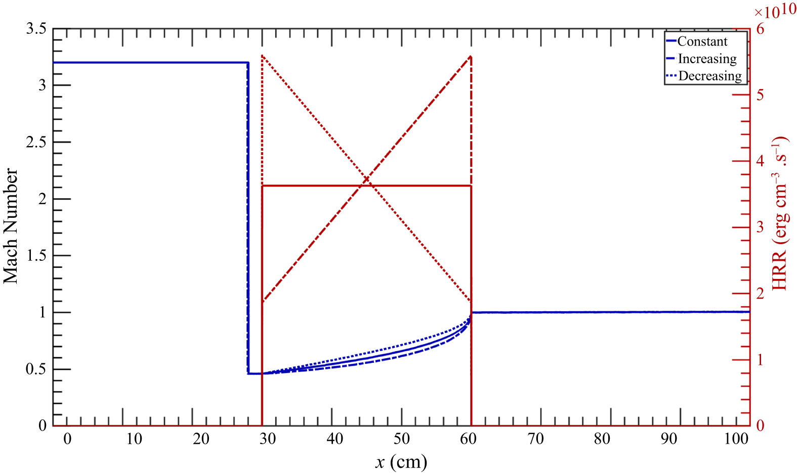
 q>q∗
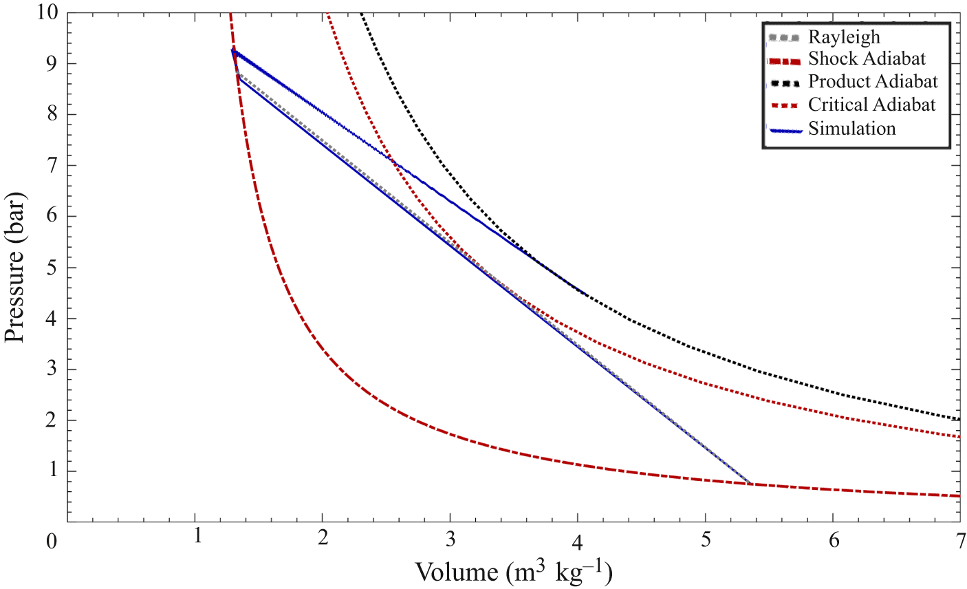


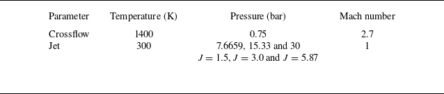


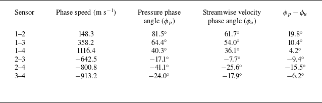


 St≈0.0115−0.016


 0∘
 ±180∘


 Open access

