2 Experimental details

The plane jet used in the present study issues from a two-dimensional contraction of a wind tunnel. Since the experiment was originally carried out by Zhou, Antonia & Chua (Reference Zhou, Antonia and Chua2005), a detailed description of the experimental conditions and measurement techniques can be found in that paper. The tunnel comprises a single inlet 15 kW centrifugal fan, which is able to deliver a maximum free stream velocity of approximately 40 m s $^{-1}$ . After the fan outlet, the air enters a settling chamber via a two-stage two-dimensional diffuser. Downstream of the settling chamber ( $1.6\times 0.9~\text{m}^{2}$ ), which includes 6 evenly spaced wire-mesh screens and a 5 mm aluminium honey comb, the flow enters a two-dimensional contraction (area ratio is 9.5) and exits in a laminar state. The contraction exit has a height $d$ of 16.5 cm and width $h=82.5$  cm (aspect ratio is 5). The longitudinal axis of the contraction is 1.2 m above the floor of the laboratory. 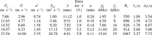The main set of measurements was made at a distance $x=36d$ downstream of the exit, at five values of the exit velocity $U_{j}$ with a one-component (spanwise) vorticity probe. The magnitude of $U_{j}$ varies approximately between $8~\text{m}~\text{s}^{-1}$ and $24~\text{m}~\text{s}^{-1}$ . Correspondingly, the Reynolds number $R_{d}=U_{j}d/\unicode[STIX]{x1D708}$ at the jet exit varies between $8.4\times 10^{4}$ and $2.6\times 10^{5}$ . The corresponding $R_{\unicode[STIX]{x1D706}}$ range is 500–1100.

The one-component vorticity probe consists of one X-wire lying in the ( $x$ , $y$ ) plane, straddled by a pair of parallel single hot-wires, each aligned in the $z$ direction. All hot-wires were etched from Wollaston (Pt-10 %Rh) wire to an active length $l_{w}$ of 200 $d_{w}$ ( $d_{w}$ is the wire diameter, here equal to 1.27  $\unicode[STIX]{x03BC}$ m) to minimize end effects. They were operated with in-house constant temperature anemometers at an overheat ratio of 1.5. Output signals from the anemometers were passed through buck and gain circuits and low-pass filtered at a cutoff frequency $f_{c}$ close to the Kolmogorov frequency $f_{K}\equiv U/2\unicode[STIX]{x03C0}\unicode[STIX]{x1D702}$ . The filtered signals were sampled (12 bit analogue-to-digital converter) at a frequency $f_{s}$ set equal to $2f_{c}$ . The record duration was in the range 60–300 s. The separation between the parallel wires $\unicode[STIX]{x0394}y$ is equal to 0.85 mm. For all the Reynolds numbers considered here, $l_{w}/\unicode[STIX]{x1D702}$ lies between 1 and 2.4 whilst $\unicode[STIX]{x0394}y/\unicode[STIX]{x1D702}$ is in the range 3.5–7.7. The main flow parameters are given in table 1. Note that the uncertainty in estimating $\unicode[STIX]{x1D706}$ is less than 4 % for all $R_{\unicode[STIX]{x1D706}}$ in table 1, which gives us confidence that the position of $\unicode[STIX]{x1D706}$ has been estimated with sufficient accuracy. It will be seen later (figures 8–11) that $\unicode[STIX]{x1D706}$ is located near the lower end of the SR. The same observation can be also made from figures 1–7 of Gotoh & Nakano (Reference Gotoh and Nakano2003) for SFPBT at $R_{\unicode[STIX]{x1D706}}=460$ . Note that $R_{\unicode[STIX]{x1D706}}$ ( $=500$ –1100) in table 1 is larger than that of Gotoh & Nakano (Reference Gotoh and Nakano2003). On the other hand, the ratio $\unicode[STIX]{x1D706}/\unicode[STIX]{x1D702}$ is in the range 46–62, which is sufficiently large to support the choice of $r=\unicode[STIX]{x1D706}$ , as discussed in the introduction.

Table 1.

Flow parameters on the axis of the plane jet.

3 Local isotropy

A key assumption of K41 and K62 is that small-scale turbulence at sufficiently high $R_{\unicode[STIX]{x1D706}}$ is statistically independent of the large scales. Kolmogorov assumed that the small scales are isotropic in space and stationary in time. Following Monin & Yaglom (Reference Monin and Yaglom2007), a well-known isotropic relation between second-order structure functions of longitudinal and transverse velocity components is given by

(3.1) $$\begin{eqnarray}\overline{(\unicode[STIX]{x1D6FF}v)^{2}}_{iso}=\left(1+\frac{r}{2}\frac{\text{d}}{\text{d}r}\right)\overline{(\unicode[STIX]{x1D6FF}u)^{2}}.\end{eqnarray}$$

The isotropic relation between third-order structure functions is also given by Monin & Yaglom (Reference Monin and Yaglom2007) (see also (Thiesset, Danaila & Antonia Reference Thiesset, Danaila and Antonia2013a )) as

(3.2) $$\begin{eqnarray}\overline{(\unicode[STIX]{x1D6FF}u)(\unicode[STIX]{x1D6FF}v)^{2}}_{iso}=\left(\frac{1}{6}\frac{\text{d}}{\text{d}r}r\overline{(\unicode[STIX]{x1D6FF}u)^{3}}\right).\end{eqnarray}$$

Figure 1 shows the ratios between calculated and measured second- and third-order structure functions at $R_{\unicode[STIX]{x1D706}}=550$ and 1067, respectively. For both the second- and third-order structure functions, the departure from local isotropy appears to be relatively small in the dissipation range ( $r^{\ast }<20$ ), the maximum departure being approximately 20 %. In the SR, although there is a systematic departure from local isotropy for both the second- and third-order structure functions, there is also an improvement in local isotropy as $R_{\unicode[STIX]{x1D706}}$ increases. The departure from local isotropy in the SR is reflected by the inequality between $\unicode[STIX]{x1D6FD}_{n}$ ( $\overline{(\unicode[STIX]{x1D6FF}v)^{n}}\sim r^{\unicode[STIX]{x1D6FD}_{n}}$ ) and $\unicode[STIX]{x1D6FC}_{n}$ (1.5). For example, $\unicode[STIX]{x1D6FD}_{4}=1.05$ , whereas $\unicode[STIX]{x1D6FC}_{4}\approx 1.34$ at $R_{\unicode[STIX]{x1D706}}=1067$ . Note that at $r=\unicode[STIX]{x1D706}$ figure 1, the departure from local isotropy is within $\pm 20\,\%$ at both the largest and smallest values of $R_{\unicode[STIX]{x1D706}}$ , thus justifying this particular choice of $r$ ( $=\unicode[STIX]{x1D706}$ ) in the analytical work of next section. We finally recall that the main focus of the present paper is to address the finite Reynolds number effect on the SR behaviour of $\overline{(\unicode[STIX]{x1D6FF}u)^{n}}$ . Evidently, it would be desirable to further investigate the FRN effect on local isotropy in the SR and the SR behaviour of the transverse structure functions by further increasing $R_{\unicode[STIX]{x1D706}}$ .

Figure 1.

Ratios of isotropic and measured second- (red) and third-order (black) structure functions in the dissipation range. ▿, $R_{\unicode[STIX]{x1D706}}=1067$ ; ▫, $R_{\unicode[STIX]{x1D706}}=550$ . Solid line indicates the isotropic ratio of 1. Dashed green lines indicate a departure of 20 % from the isotropic value of one. Arrowed horizontal line indicates the extent of the scaling range. The vertical arrows indicate the magnitudes of the Taylor microscale ( $\unicode[STIX]{x1D706}/\unicode[STIX]{x1D702}$ ) at $R_{\unicode[STIX]{x1D706}}=550$ (left) and 1067 (right) respectively.

4 Effect of $I_{u}(r)$ on $\overline{(\unicode[STIX]{x1D6FF}u^{\ast })^{3}}$ at $r=\unicode[STIX]{x1D706}$

We first discuss the different forms of the term $I_{u}(r)$ in (1.2) in different types of flows.

(i) In decaying HIT, $I_{u}(r)$ is the streamwise advection term for $\overline{(\unicode[STIX]{x1D6FF}u)^{2}}$ and is given by (e.g. Danaila et al. Reference Danaila, Anselmet, Zhou and Antonia1999; Antonia et al. Reference Antonia, Zhou, Danaila and Anselmet2000b ; Danaila et al. Reference Danaila, Anselmet and Antonia2002, Reference Danaila, Antonia and Burattini2004)

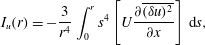(4.1) $$\begin{eqnarray}I_{u}(r)=-\frac{3}{r^{4}}\int _{0}^{r}s^{4}\left[U\frac{\unicode[STIX]{x2202}\overline{(\unicode[STIX]{x1D6FF}u)^{2}}}{\unicode[STIX]{x2202}x}\right]\,\text{d}s,\end{eqnarray}$$

where s is a dummy variable, identifiable with the separation along $x$ and $U$ is the (constant) mean velocity in the $x$ direction.

(ii) Along the axis in the far field of an axisymmetric jet flow where the flow satisfies self-preservation, $I_{u}(r)$ , which includes a streamwise advection term for $\overline{(\unicode[STIX]{x1D6FF}u)^{2}}$ and a production term, is given by (Burattini et al. Reference Burattini, Antonia and Danaila2005b ; Thiesset et al. Reference Thiesset, Antonia and Djenidi2014)

(4.2) $$\begin{eqnarray}I_{u}(r)=-\frac{3}{r^{4}}\int _{0}^{r}s^{4}\left[U\frac{\unicode[STIX]{x2202}\overline{(\unicode[STIX]{x1D6FF}u)^{2}}}{\unicode[STIX]{x2202}x}+2\left[\overline{(\unicode[STIX]{x1D6FF}u)^{2}}-\overline{(\unicode[STIX]{x1D6FF}v)^{2}}\right]\frac{\unicode[STIX]{x2202}U}{\unicode[STIX]{x2202}x}\right]\,\text{d}s.\end{eqnarray}$$

(iii) Along the centreline of a fully developed channel flow, $I_{u}(r)$ , which arises from the turbulent transport of $(\unicode[STIX]{x1D6FF}u)^{2}$ by the wall-normal velocity fluctuation $v$ , is given by (Danaila et al. Reference Danaila, Anselmet, Zhou and Antonia2001)

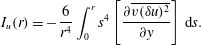(4.3) $$\begin{eqnarray}I_{u}(r)=-\frac{6}{r^{4}}\int _{0}^{r}s^{4}\left[\frac{\unicode[STIX]{x2202}\overline{v(\unicode[STIX]{x1D6FF}u)^{2}}}{\unicode[STIX]{x2202}y}\right]\,\text{d}s.\end{eqnarray}$$

(iv) For SFPBT, the forcing is usually concentrated at very low wavenumbers (i.e. very large scales). For example, $I_{u}(r)$ is given by (Fukayama et al. Reference Fukayama, Oyamada, Nakano, Gotoh and Yamamoto2000)

(4.4) $$\begin{eqnarray}I_{u}(r)={\textstyle \frac{2}{21}}\unicode[STIX]{x1D716}_{in}(k_{e}r)^{2}r,\end{eqnarray}$$

where $\unicode[STIX]{x1D716}_{in}$ is the energy input rate due to external random forces concentrated at wavenumber $k\sim k_{e}$ .

The scale by scale energy budget equations, with the various forms of $I_{u}$ , have already been satisfactorily validated over the range $\unicode[STIX]{x1D702}\leqslant r\leqslant L$ against experimental and numerical data in various turbulent flows. This has been reported for grid turbulence (Danaila et al. Reference Danaila, Anselmet, Zhou and Antonia1999; Antonia et al. Reference Antonia, Zhou, Danaila and Anselmet2000b ; Danaila et al. Reference Danaila, Anselmet and Antonia2002, Reference Danaila, Antonia and Burattini2004; Antonia & Burattini Reference Antonia and Burattini2006), along the axis in the far field of an axisymmetric jet flow (Danaila et al. Reference Danaila, Antonia and Burattini2004; Burattini, Antonia & Danaila Reference Burattini, Antonia and Danaila2005a ), along the centreline of a fully developed channel flow (Danaila et al. Reference Danaila, Anselmet, Zhou and Antonia2001, Reference Danaila, Anselmet and Antonia2002; Fukayama et al. Reference Fukayama, Oyamada, Nakano, Gotoh and Yamamoto2000). For this reason, and to limit the length of this present paper, we only focus on the variation of $I_{u}(r)$ at $r=\unicode[STIX]{x1D706}$ on $R_{\unicode[STIX]{x1D706}}$ .

After dividing by $u_{K}^{3}$ and taking $r=\unicode[STIX]{x1D706}$ , the term on the right-hand side of (1.2) becomes

(4.5) $$\begin{eqnarray}\frac{4}{5u_{K}^{3}}\overline{\unicode[STIX]{x1D716}}r=\frac{4}{5}\unicode[STIX]{x1D706}^{\ast },\end{eqnarray}$$

while the second and third terms on the left-hand side of (1.2) become

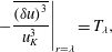(4.6) $$\begin{eqnarray}\displaystyle & \displaystyle \left.-\frac{\overline{(\unicode[STIX]{x1D6FF}u)^{3}}}{u_{K}^{3}}\right|_{r=\unicode[STIX]{x1D706}}=T_{\unicode[STIX]{x1D706}}, & \displaystyle\end{eqnarray}$$

(4.7) $$\begin{eqnarray}\displaystyle & \displaystyle \frac{6\unicode[STIX]{x1D708}}{u_{K}^{3}}\frac{\unicode[STIX]{x2202}\overline{(\unicode[STIX]{x1D6FF}u)^{2}}}{\unicode[STIX]{x2202}r}=\left.6\frac{\unicode[STIX]{x2202}\overline{(\unicode[STIX]{x1D6FF}u^{\ast })^{2}}}{\unicode[STIX]{x2202}r^{\ast }}\right|_{r=\unicode[STIX]{x1D706}}=V_{\unicode[STIX]{x1D706}}. & \displaystyle\end{eqnarray}$$

After normalizing by Kolmogorov scales and taking $r=\unicode[STIX]{x1D706}$ , $I_{u}(r)$ can be written, for decaying HIT, as

(4.8) $$\begin{eqnarray}I_{u}(\unicode[STIX]{x1D706}^{\ast })=-\frac{3}{\unicode[STIX]{x1D706}^{\ast 4}}\int _{0}^{\unicode[STIX]{x1D706}^{\ast }}s^{\ast 4}\left[U^{\ast }\frac{\unicode[STIX]{x2202}\overline{(\unicode[STIX]{x1D6FF}u^{\ast })^{2}}}{\unicode[STIX]{x2202}x^{\ast }}\right]\,\text{d}s^{\ast }.\end{eqnarray}$$

$I_{u}(\unicode[STIX]{x1D706}^{\ast })$ is not written here for other flows since it is simply the normalized form of (4.2)–(4.4).

It is worth recalling that, by assuming self-preservation for decaying HIT, $I_{u}(\unicode[STIX]{x1D706}^{\ast })$ can also be recast as

(4.9) $$\begin{eqnarray}I_{u}(\unicode[STIX]{x1D706}^{\ast })=\frac{\sqrt{15}}{2}\left(\frac{n-1}{n}\right)\left(\int _{0}^{\unicode[STIX]{x1D706}^{\ast }}s^{\ast 5}\frac{\unicode[STIX]{x2202}\overline{(\unicode[STIX]{x1D6FF}u^{\ast })^{2}}}{\unicode[STIX]{x2202}r^{\ast }}\,\text{d}s^{\ast }+2\int _{0}^{\unicode[STIX]{x1D706}^{\ast }}s^{\ast 4}\overline{(\unicode[STIX]{x1D6FF}u^{\ast })^{2}}\,\text{d}s^{\ast }\right)\frac{1}{\unicode[STIX]{x1D706}^{\ast 4}R_{\unicode[STIX]{x1D706}}},\end{eqnarray}$$

where $n$ is the power-law decay rate for $\overline{u^{2}}$ , viz. $\overline{u^{2}}\sim x^{-n}$ . Strictly, complete self-preservation or self-preservation at all scales is tenable in decaying HIT only when $R_{\unicode[STIX]{x1D706}}\rightarrow \infty$ (Djenidi & Antonia Reference Djenidi and Antonia2015). However, similarity based on Kolmogorov scales should be applicable in some regions of any turbulent flow when $r$ is sufficiently small, e.g. Antonia, Djenidi & Danaila (Reference Antonia, Djenidi and Danaila2014). This justifies the use of Kolmogorov scales in (4.9) at $r=\unicode[STIX]{x1D706}$ . Along the axis in the far field of the round jet, $I_{u}(r^{\ast })$ can be also recast as

(4.10) $$\begin{eqnarray}I_{u}(\unicode[STIX]{x1D706}^{\ast })=\left(\frac{3\sqrt{15}}{2+R}\right)R_{\unicode[STIX]{x1D706}}^{-1}(\unicode[STIX]{x1D6E4}_{1}^{\ast }+4\unicode[STIX]{x1D6E4}_{2}^{\ast }-2\unicode[STIX]{x1D6E4}_{3}^{\ast })r^{\ast -4},\end{eqnarray}$$

where $\unicode[STIX]{x1D6E4}_{1}^{\ast }=\int _{0}^{r^{\ast }}s^{\ast 5}\unicode[STIX]{x2202}\overline{(\unicode[STIX]{x1D6FF}u^{\ast })^{2}}/\unicode[STIX]{x2202}r^{\ast }\text{d}s^{\ast }$ , $\unicode[STIX]{x1D6E4}_{2}^{\ast }=\int _{0}^{r^{\ast }}s^{\ast 4}\overline{(\unicode[STIX]{x1D6FF}u^{\ast })^{2}}\text{d}s^{\ast }$ , $\unicode[STIX]{x1D6E4}_{3}^{\ast }=\int _{0}^{r^{\ast }}s^{\ast 4}\overline{(\unicode[STIX]{x1D6FF}v^{\ast })^{2}}\text{d}s^{\ast }$ (see also the first term on the left-hand side of (2.17) in Thiesset et al. (Reference Thiesset, Antonia and Djenidi2014)), at all scales, not only at $r=\unicode[STIX]{x1D706}$ since complete self-preservation is satisfied.

Finally, equation (1.2) can be written, when $r=\unicode[STIX]{x1D706}$ , as

(4.11) $$\begin{eqnarray}I_{u}(\unicode[STIX]{x1D706}^{\ast })+T_{\unicode[STIX]{x1D706}}+V_{\unicode[STIX]{x1D706}}={\textstyle \frac{4}{5}}\unicode[STIX]{x1D706}^{\ast },\end{eqnarray}$$

where $I_{u}(\unicode[STIX]{x1D706}^{\ast })$ differs from flow to flow and possibly from position to position in a given flow. The main objective for deriving (4.11) is to assess the influence of $I_{u}(\unicode[STIX]{x1D706}^{\ast })$ on $\overline{(\unicode[STIX]{x1D6FF}u^{\ast })^{n}}$ ( $n=2$ and 3 at $r=\unicode[STIX]{x1D706}$ , $-\overline{(\unicode[STIX]{x1D6FF}u^{\ast })^{3}}_{r=\unicode[STIX]{x1D706}}=T_{\unicode[STIX]{x1D706}}$ ) in the turbulent flows mentioned above, i.e. decaying HIT, the centreline of a fully developed channel flow, the axis of a turbulent round jet and SFPBT, for as wide a range of $R_{\unicode[STIX]{x1D706}}$ .

5 Results for $\overline{(\unicode[STIX]{x1D6FF}u^{\ast })^{n}}$ ( $n=2$ and 3 at $r=\unicode[STIX]{x1D706}$ , $-\overline{(\unicode[STIX]{x1D6FF}u^{\ast })^{3}}_{r=\unicode[STIX]{x1D706}}=T_{\unicode[STIX]{x1D706}}$ )

Figure 2.

Dependence of $I_{u}(\unicode[STIX]{x1D706}^{\ast })$ on $R_{\unicode[STIX]{x1D706}}$ in different flows. ▪, grid turbulence (Zhou & Antonia Reference Zhou and Antonia2000); ○ and ▫ correspond to the data in circular and square cylinder wakes respectively (Antonia, Zhou & Romano Reference Antonia, Zhou and Romano2002b ); SFPBT: ●, (Fukayama et al. Reference Fukayama, Oyamada, Nakano, Gotoh and Yamamoto2000);  $\times$ , (Gotoh, Fukayama & Nakano Reference Gotoh, Fukayama and Nakano2002); ▼, channel centreline (Danaila et al. Reference Danaila, Anselmet, Zhou and Antonia2001); ♦, circular jet axis, estimates from the data of Xu, Antonia & Rajagopalan (Reference Xu, Antonia and Rajagopalan2001). The solid and dash-dotted curves correspond to the model for decaying HIT (Antonia & Burattini Reference Antonia and Burattini2006) and jet axis. The horizontal dashed line indicates a value of zero, i.e. the value expected when there is no effect from the large scales.

Estimates of $I_{u}(\unicode[STIX]{x1D706}^{\ast })$ for the different flows considered in § 4 have been obtained with experimental and numerical data and are shown in figure 2. Also included are estimates inferred from the parameterized form of $\overline{(\unicode[STIX]{x1D6FF}u^{\ast })^{2}}$ in decaying HIT (Kurien & Sreenivasan Reference Kurien and Sreenivasan2000; Antonia et al. Reference Antonia, Smalley, Zhou, Anselmet and Danaila2003; Antonia & Burattini Reference Antonia and Burattini2006), viz.

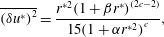(5.1) $$\begin{eqnarray}\overline{(\unicode[STIX]{x1D6FF}u^{\ast })^{2}}=\frac{r^{\ast 2}(1+\unicode[STIX]{x1D6FD}r^{\ast })^{(2c-2)}}{15(1+\unicode[STIX]{x1D6FC}r^{\ast 2})^{c}},\end{eqnarray}$$

where $\unicode[STIX]{x1D6FC}$ ( $=30^{-3/2}$ ) is a measure of the cross-over between the dissipative and scaling ranges, $c=1-\unicode[STIX]{x1D701}/2$ ( $\unicode[STIX]{x1D701}=2/3$ is the scaling range exponent without intermittency correction) and $\unicode[STIX]{x1D6FD}=L^{\ast -1}$ ( $L$ is the integral length scale). For isotropic turbulence, $\unicode[STIX]{x1D706}^{\ast }=15^{1/4}R_{\unicode[STIX]{x1D706}}^{1/2}$ and $L^{\ast }=C_{\unicode[STIX]{x1D716}}15^{-3/4}R_{\unicode[STIX]{x1D706}}^{3/2}$ ( $C_{\unicode[STIX]{x1D716}}=1$ for decaying HIT). Here the correction for $\unicode[STIX]{x1D701}$ is not essential for estimating $I_{u}(\unicode[STIX]{x1D706}^{\ast })$ , e.g. distributions of $I_{u}(\unicode[STIX]{x1D706}^{\ast })$ which correspond to $\unicode[STIX]{x1D701}=2/3$ and $\unicode[STIX]{x1D701}=0.71$ , the value used by Anselmet et al. (Reference Anselmet, Gagne, Hopfinger and Antonia1984), are almost identical (they are not shown here). This model has been tested in some detail by Antonia & Burattini (Reference Antonia and Burattini2006); they showed that $R_{\unicode[STIX]{x1D706}}$ needs to exceed $10^{6}$ before the IR is established unequivocally. Note that an earlier version of this model was also tested extensively (Antonia, Pearson & Zhou Reference Antonia, Pearson and Zhou2002a ) in other flows. Following Monin & Yaglom (Reference Monin and Yaglom2007), the well-known isotropic relation between $\overline{(\unicode[STIX]{x1D6FF}u)^{2}}$ and $\overline{(\unicode[STIX]{x1D6FF}v)^{2}}$ is given by (3.1). Relations (5.1) and (3.1) allow $I_{u}(\unicode[STIX]{x1D706}^{\ast })$ to be estimated for the flow along the axis of a round jet. All the parameters are chosen to be the same as in decaying HIT except for $C_{\unicode[STIX]{x1D716}}$ which is 0.75 (Mi, Xu & Zhou Reference Mi, Xu and Zhou2013); note that $C_{\unicode[STIX]{x1D716}}$ has a negligible effect on the estimate of $I_{u}(\unicode[STIX]{x1D706}^{\ast })$ . Since the one-point energy budget in the intermediate wake of either a circular cylinder (Thiesset, Antonia & Danaila Reference Thiesset, Antonia and Danaila2013b ) or square cylinder (Lefeuvre (2014), private communication) is quite similar to that for decaying HIT, estimates of $I_{u}(\unicode[STIX]{x1D706}^{\ast })$ in these two flows at $x/d=70$ , where $d$ is the diameter of the cylinder, are also shown; these values are estimated from the data of Antonia et al. (Reference Antonia, Zhou and Romano2002b ).

Figure 2 indicates that $I_{u}(\unicode[STIX]{x1D706}^{\ast })$ varies markedly among different flows. For example, it is smallest, if not negligible, for SFPBT, suggesting that this flow is most ideal for examining scaling exponents of $\overline{(\unicode[STIX]{x1D6FF}u)^{3}}$ in the scaling range. Indeed, Moisy, Tabeling & Willaime (Reference Moisy, Tabeling and Willaime1999), Antonia & Burattini (Reference Antonia and Burattini2006), Gotoh & Watanabe (Reference Gotoh and Watanabe2015) showed that $R_{\unicode[STIX]{x1D706}}\sim 10^{3}$ appears to be sufficient for the K41 $4/5$ law is approached in this flow. Along the centreline of a fully developed channel flow, $I_{u}(\unicode[STIX]{x1D706}^{\ast })$ is largest of all cases considered here. For decaying HIT and on the cylinder wake axis, the magnitude of $I_{u}(\unicode[STIX]{x1D706}^{\ast })$ is in reasonable agreement with the prediction from the model of (5.1) for decaying HIT. The prediction from the model for the round jet, in good agreement with the magnitude of $I_{u}(\unicode[STIX]{x1D706}^{\ast })$ estimated from the data of Xu et al. (Reference Xu, Antonia and Rajagopalan2001), is smaller than in decaying HIT since an additional production term $I_{u}(r)$ emerges on the left-hand side of (4.2). In order to show how large a value of $R_{\unicode[STIX]{x1D706}}$ is needed for $I_{u}(\unicode[STIX]{x1D706}^{\ast })$ to be negligible, figure 3(a) shows the predictions from the models for the round jet and decaying HIT up to $R_{\unicode[STIX]{x1D706}}=10^{8}$ . It is clear from this figure that, for both flows, $R_{\unicode[STIX]{x1D706}}$ should exceed $10^{8}$ for $I_{u}(\unicode[STIX]{x1D706}^{\ast })$ to become negligible. For $I_{u}(\unicode[STIX]{x1D706}^{\ast })/\unicode[STIX]{x1D706}^{\ast }$ in figure 3(b), it approaches zero when $R_{\unicode[STIX]{x1D706}}>10^{5}$ , beyond which the K41 $4/5$ law is approached (Antonia & Burattini Reference Antonia and Burattini2006). It is clear that, at $r=\unicode[STIX]{x1D706}$ (a scale which lies near the start of the SR), the contribution of the large-scale terms to the scale by scale energy budget in decaying-type flows can persist at high $R_{\unicode[STIX]{x1D706}}$ and this contribution is expected to become larger as $r$ increases beyond $r=\unicode[STIX]{x1D706}$ in the SR. However, it is well known that for laboratory measurements, on the other hand, $R_{\unicode[STIX]{x1D706}}$ hardly ever exceeds $10^{3}$ ; exceptions are the experiments of Tabeling et al. (Reference Tabeling, Zocchi, Belin, Maurer and Willaime1996) and Belin et al. (Reference Belin, Maurer, Tabeling and Willaime1997) who used low temperature helium in a cylindrical container between two counter-rotating disks. In this flow, the maximum value of $R_{\unicode[STIX]{x1D706}}$ reached 5000.

Figure 3.

Dependence of $I_{u}(\unicode[STIX]{x1D706}^{\ast })$ (a) and $I_{u}(\unicode[STIX]{x1D706}^{\ast })/\unicode[STIX]{x1D706}^{\ast }$ (b) on $R_{\unicode[STIX]{x1D706}}$ in decaying HIT (solid curve) and along the axis of a circular jet (dashed curve). Both curves are estimated from the models ((5.1) is introduced in (4.9) to obtain $I_{u}(\unicode[STIX]{x1D706}^{\ast })$ in decaying HIT; (5.1) and (3.1) are introduced in (4.10) to obtain $I_{u}(\unicode[STIX]{x1D706}^{\ast })$ along the axis of a circular jet). The horizontal dashed line indicates a value of zero, i.e. the value expected when there is no effect from the large scales.

Figure 4.

Dependence of $V_{\unicode[STIX]{x1D706}}$ , the normalized ‘viscous’ term in (1.2), on $R_{\unicode[STIX]{x1D706}}$ in different flows. ▪, grid turbulence (Zhou & Antonia Reference Zhou and Antonia2000); ○ and ▫ correspond to the data in circular and square cylinder wake respectively (Antonia et al. Reference Antonia, Zhou and Romano2002b ); ▼, channel centreline (Tang et al. Reference Tang, Antonia, Djenidi, Abe, Zhou, Danaila and Zhou2015a ); ♦, pipe axis (Antonia & Pearson Reference Antonia and Pearson2000); SFPBT: ●, Fukayama et al. (Reference Fukayama, Oyamada, Nakano, Gotoh and Yamamoto2000);  $\times$ , Gotoh et al. (Reference Gotoh, Fukayama and Nakano2002). The solid curve corresponds to the model for decaying HIT (Antonia & Burattini Reference Antonia and Burattini2006). The horizontal dashed line indicates a value of zero, i.e. the value expected when there is no effect from the small scales.

Estimates of $V_{\unicode[STIX]{x1D706}}$ for the flows considered in figure 2 are shown in figure 4. Also included are estimates inferred from (5.1). Since the one-point energy budget along the axis of a pipe is quite similar to that on the channel centreline, estimates of $V_{\unicode[STIX]{x1D706}}$ on the axis of the pipe are also shown (Antonia & Pearson Reference Antonia and Pearson2000). In contrast to $I_{u}(\unicode[STIX]{x1D706}^{\ast })$ in figure 2, the values of $V_{\unicode[STIX]{x1D706}}$ (see figure 4) in different flows are closer together and appear to be independent of the flow. However, it is somewhat surprising that, for decaying-type flows, $V_{\unicode[STIX]{x1D706}}$ is close to $I_{u}(\unicode[STIX]{x1D706}^{\ast })$ (see figure 2) suggesting that the viscous term and the large-scale term $I_{u}(\unicode[STIX]{x1D706}^{\ast })$ have comparable contributions (see also figure 7) to the scale by scale energy budget equation in these flows at $r=\unicode[STIX]{x1D706}$ ; this can also be seen from the results of Antonia & Burattini (Reference Antonia and Burattini2006). In SFPBT, the viscous term is significantly larger than the large-scale forcing term $I_{u}(\unicode[STIX]{x1D706}^{\ast })$ (i.e. $I_{u}(\unicode[STIX]{x1D706}^{\ast })<V_{\unicode[STIX]{x1D706}}$ ) when the external forcing is concentrated at very low wavenumbers (i.e. very large scales). In contrast, on the centreline of a fully developed channel flow, the large-scale term $I_{u}(\unicode[STIX]{x1D706}^{\ast })$ makes a larger contribution to the energy budget than the viscous term at low $R_{\unicode[STIX]{x1D706}}$ . Estimates from the model (5.1) collapse reasonably well with the data from grid turbulence over the range $30<R_{\unicode[STIX]{x1D706}}<100$ . In similar manner to $I_{u}(\unicode[STIX]{x1D706}^{\ast })$ (figure 2), figure 4 shows that $R_{\unicode[STIX]{x1D706}}$ also needs to be large before $V_{\unicode[STIX]{x1D706}}$ can be neglected, suggesting that the viscous term contributes to the budget at $r=\unicode[STIX]{x1D706}$ from small to moderate $R_{\unicode[STIX]{x1D706}}$ .

The main message of figure 2 is that, at $r=\unicode[STIX]{x1D706}$ , the contributions from the large-scale forcing term to the scale by scale energy budget equation differ from flow to flow at small to moderate $R_{\unicode[STIX]{x1D706}}$ . Thus, $T_{\unicode[STIX]{x1D706}}$ (see (4.6)) at $r=\unicode[STIX]{x1D706}$ may also differ from flow to flow at small to moderate $R_{\unicode[STIX]{x1D706}}$ . Although it appears to be independent of the flow, the viscous term has comparable contributions to that of the large-scale term in decaying-type flows. The effect of $I_{u}(\unicode[STIX]{x1D706}^{\ast })$ on $T_{\unicode[STIX]{x1D706}}$ and $\overline{(\unicode[STIX]{x1D6FF}u^{\ast })^{2}}$ is discussed below.

Figure 5.

$R_{\unicode[STIX]{x1D706}}$ dependence of $\overline{(\unicode[STIX]{x1D6FF}u^{\ast })^{2}}$ in different flows at $r=\unicode[STIX]{x1D706}$ . ▪, grid turbulence (Zhou & Antonia Reference Zhou and Antonia2000); ▼, channel centreline (Tang et al. Reference Tang, Antonia, Djenidi, Abe, Zhou, Danaila and Zhou2015a ); ○, pipe axis (Antonia & Pearson Reference Antonia and Pearson2000).

Figure 6.

(a) $R_{\unicode[STIX]{x1D706}}$ dependence of $T_{\unicode[STIX]{x1D706}}$ ( $=-\overline{(\unicode[STIX]{x1D6FF}u^{\ast })^{3}}|_{r=\unicode[STIX]{x1D706}}$ ) in different flows. ▪, grid turbulence (Zhou & Antonia Reference Zhou and Antonia2000); SFPBT: ●, Fukayama et al. (Reference Fukayama, Oyamada, Nakano, Gotoh and Yamamoto2000); ▼, channel centreline (Tang et al. Reference Tang, Antonia, Djenidi, Abe, Zhou, Danaila and Zhou2015a ); ○, pipe axis (Antonia & Pearson Reference Antonia and Pearson2000). (b)  $T_{\unicode[STIX]{x1D706}}/\unicode[STIX]{x1D706}^{\ast }$ ( $=-\overline{(\unicode[STIX]{x1D6FF}u^{\ast })^{3}}|_{r=\unicode[STIX]{x1D706}}/\unicode[STIX]{x1D706}^{\ast }$ ) symbols correspond to (a).

Figure 5 shows $\overline{(\unicode[STIX]{x1D6FF}u^{\ast })^{2}}$ for three of the flows considered in § 4. No data are available at low $R_{\unicode[STIX]{x1D706}}$ for SFPBT and along the jet axis. Also included are estimates inferred from the data measured along the axis of a pipe. It is clear that $\overline{(\unicode[STIX]{x1D6FF}u^{\ast })^{2}}$ , like the viscous term $V_{\unicode[STIX]{x1D706}}$ (see figure 4), is nearly independent of the flow.

As shown in figures 2 and 4, and although $V_{\unicode[STIX]{x1D706}}$ appears to be independent of the flow, $I_{u}(\unicode[STIX]{x1D706}^{\ast })$ differs from flow to flow at small to moderate $R_{\unicode[STIX]{x1D706}}$ . Accordingly, $T_{\unicode[STIX]{x1D706}}$ also differs in different flows over the same range of $R_{\unicode[STIX]{x1D706}}$ . The smallest values of $T_{\unicode[STIX]{x1D706}}$ occur on the axis of the pipe. In decaying grid turbulence, $T_{\unicode[STIX]{x1D706}}$ is larger than along the channel centreline, which is consistent with the smaller values of $I_{u}(\unicode[STIX]{x1D706}^{\ast })$ (figure 2) in the former flow. The largest value occurs for SFPBT; this is consistent with the smallest values of $I_{u}(\unicode[STIX]{x1D706}^{\ast })$ in figure 2. We should stress that $T_{\unicode[STIX]{x1D706}}/\unicode[STIX]{x1D706}^{\ast }$ must approach the K41 $4/5$ law as $R_{\unicode[STIX]{x1D706}}$ continues to increase (Antonia & Burattini Reference Antonia and Burattini2006) and the way the $4/5$ law is approached should become flow dependent as suggested in figure 6(b).

In order to highlight the effect of the small scales and the large scales on $T_{\unicode[STIX]{x1D706}}/\unicode[STIX]{x1D706}^{\ast }$ , the distributions in figures 3(b), 4, and 6(b) are replotted in figure 7. It can be seen from this figure that $T_{\unicode[STIX]{x1D706}}/\unicode[STIX]{x1D706}^{\ast }$ must eventually dominate over the other two terms (viscous term and large-scale term) as $R_{\unicode[STIX]{x1D706}}$ becomes large enough. Overall, figure 7 strongly supports the idea that the large-scale forcing (or FRN effect), which differs from flow to flow, has a significant effect on $T_{\unicode[STIX]{x1D706}}$ at small to moderate $R_{\unicode[STIX]{x1D706}}$ . This effect is expected to be amplified as $r$ increases beyond $r=\unicode[STIX]{x1D706}$ in the SR. It is similar to the FRN effect on the SR power-law exponents of $\unicode[STIX]{x1D719}_{u}(k_{1})$ , $S_{\unicode[STIX]{x1D6FF}u}$ and $E_{p}(k_{1})$ as mentioned in the Introduction. In the next section, we examine the FRN effect on the SR scaling exponents of the longitudinal velocity structure functions at large $R_{\unicode[STIX]{x1D706}}$ ( $=500$ –1100) on the axis of a plane jet.

Figure 7.

Dependence of $I_{u}(\unicode[STIX]{x1D706}^{\ast })/\unicode[STIX]{x1D706}^{\ast }$ , $T_{\unicode[STIX]{x1D706}}/\unicode[STIX]{x1D706}^{\ast }$ (the symbols are as in figure 6), and $V_{\unicode[STIX]{x1D706}}/\unicode[STIX]{x1D706}^{\ast }$ on $R_{\unicode[STIX]{x1D706}}$ in different flows. The horizontal dashed line indicates a value of zero, i.e. the value expected when there is no effect from the small scales and the large scales.

6 SR scaling exponents of velocity structure functions

In §§ 4 and 5, we have focused on low-order moments because there is an analytical framework, based on (1.2), to describe the relation between $\overline{(\unicode[STIX]{x1D6FF}u)^{2}}$ and $\overline{(\unicode[STIX]{x1D6FF}u)^{3}}$ . This section will focus primarily on the higher-order moments and the SR scaling exponents of $\overline{(\unicode[STIX]{x1D6FF}u)^{n}}$ . For the higher-order moments, it would be desirable to consider their transport equations which may allow an analytical estimate of the large-scale forcing effect (or FRN effect) on $\overline{(\unicode[STIX]{x1D6FF}u)^{n}}$ , as is done in §§ 4 and 5 for low-order moments. Although these equations are available, e.g. Hill (Reference Hill2001), evaluating the large-scale forcing effect is not straightforward. For example, the equation relating third- and fourth-order moments involve a pressure gradient velocity–velocity structure function, which we are only able to evaluate by making further assumptions. For this reason, we focus in this section on the SR behaviour of $\overline{(\unicode[STIX]{x1D6FF}u)^{n}}$ although transport equations for $n>2$ are outside the scope of this paper.

6.1 Plane and circular jets

Figures 8–10 show the fourth-, sixth- and eighth-order structure functions in the scaling range measured on the axis of a plane jet at $R_{\unicode[STIX]{x1D706}}=550$ (red) and 1067 (black), respectively. For clarity, distributions for only two values of $R_{\unicode[STIX]{x1D706}}$ are shown but we emphasize that the variation of $\overline{(\unicode[STIX]{x1D6FF}u^{\ast })^{n}}$ with $R_{\unicode[STIX]{x1D706}}$ is systematic for all values of $n$ . In each case, dashed lines are least squares fits across the SR: $60<r^{\ast }<350$ and $70<r^{\ast }<400$ for $R_{\unicode[STIX]{x1D706}}=550$ and 1067, respectively. For the purpose of comparison, the SR at each $R_{\unicode[STIX]{x1D706}}$ is fixed ( $65<r^{\ast }<400$ , see figure 11). There is a clear $R_{\unicode[STIX]{x1D706}}$ dependence of the scaling exponents for all the fourth-, sixth- and eighth-order structure functions. Figure 11 shows compensated fourth-, sixth- and eighth-order structure functions which correspond to figures 8–10, i.e. $\overline{(\unicode[STIX]{x1D6FF}u^{\ast })^{4}}r^{\ast -1.24}$ and $\overline{(\unicode[STIX]{x1D6FF}u^{\ast })^{4}}r^{\ast -1.34}$ (solid curves), $\overline{(\unicode[STIX]{x1D6FF}u^{\ast })^{6}}r^{\ast -1.66}$ and $\overline{(\unicode[STIX]{x1D6FF}u^{\ast })^{6}}r^{\ast -1.87}$ (dashed curves), $\overline{(\unicode[STIX]{x1D6FF}u^{\ast })^{8}}r^{\ast -1.95}$ and $\overline{(\unicode[STIX]{x1D6FF}u^{\ast })^{8}}r^{\ast -2.45}$ (dash-dotted curves). It can be seen from this figure that all distributions exhibit an approximate plateau in the SR, thus confirming the $R_{\unicode[STIX]{x1D706}}$ dependence of the scaling exponents for all the $4\text{th}$ , $6\text{th}$ and $8\text{th}$ -order structure functions shown in figures 8–10. Also included in figure 11 are the distributions of $\overline{(\unicode[STIX]{x1D6FF}u^{\ast })^{2}}r^{\ast -2/3}$ and $\overline{(\unicode[STIX]{x1D6FF}u^{\ast })^{3}}r^{\ast -\unicode[STIX]{x1D6FC}_{3}}$ ( $\unicode[STIX]{x1D6FC}_{3}=0.94$ and 1) at $R_{\unicode[STIX]{x1D706}}=550$ and 1067, respectively. As expected, the SR value for $\overline{(\unicode[STIX]{x1D6FF}u^{\ast })^{3}}$ approaches $4/5$ (K41) as $R_{\unicode[STIX]{x1D706}}$ increases. $\overline{(\unicode[STIX]{x1D6FF}u^{\ast })^{2}}r^{\ast -2/3}$ also exhibits an approximate plateau (both for the present data and the data of Anselmet et al. (Reference Anselmet, Gagne, Hopfinger and Antonia1984)) on the axis of a circular jet, suggesting a $R_{\unicode[STIX]{x1D706}}$ independence of the exponent for $\overline{(\unicode[STIX]{x1D6FF}u^{\ast })^{2}}$ over the present $R_{\unicode[STIX]{x1D706}}$ range. Note that the value of $2/3$ has been obtained by the same method used to determine all the other exponents $\unicode[STIX]{x1D6FC}_{n}$ , i.e. by visually choosing the value of $\unicode[STIX]{x1D6FC}_{2}$ which gives the ‘best’ plateau when plotting $\overline{(\unicode[STIX]{x1D6FF}u^{\ast })^{2}}r^{\ast -\unicode[STIX]{x1D6FC}_{2}}$ versus $r^{\ast }$ . A slightly larger magnitude ( ${\approx}0.7$ ), constant over this range of $R_{\unicode[STIX]{x1D706}}$ , was estimated by Antonia, Pearson & Zhou (Reference Antonia, Pearson and Zhou2000a ) using the same plane jet data after fitting the measured values of $\overline{(\unicode[STIX]{x1D6FF}u)^{2}}$ to the relation for $\overline{(\unicode[STIX]{x1D6FF}u)^{2}}$ developed by Batchelor (Reference Batchelor1951), viz. equation (4.1) with $\unicode[STIX]{x1D6FD}=0$ , to describe both the dissipative and scaling ranges. Clearly, the magnitude of $\unicode[STIX]{x1D6FC}_{2}$ shows a sensitivity to the method used for its determination. With the present method, there is no collapse in the SR (figure 11), suggesting that the Kolmogorov constant $C_{K}$ ( $\overline{(\unicode[STIX]{x1D6FF}u^{\ast })^{2}}=C_{K}r^{\ast 2/3}$ ) has not yet been attained by the data. Note that the FRN effect on the low-order moments of $\overline{(\unicode[STIX]{x1D6FF}u^{\ast })^{n}}$ is consistent with the observations by Pearson & Antonia (Reference Pearson and Antonia2001) over a large range of $R_{\unicode[STIX]{x1D706}}$ ( $40<R_{\unicode[STIX]{x1D706}}<4250$ ). Although not shown here, the $R_{\unicode[STIX]{x1D706}}$ dependence of the SR exponents for the fifth- and seventh-order structure functions is also observed. This underlines that the FRN effect across the SR must be assessed carefully before attempting to test either K41 or K62.

Figure 8.

Fourth-order structure functions for $R_{\unicode[STIX]{x1D706}}=550$ (red) and 1067 (black). Dashed lines ( ${\sim}r^{\ast 1.24}$ and ${\sim}r^{\ast 1.34}$ ) are least squares fits over the SR, corresponding to $R_{\unicode[STIX]{x1D706}}=550$ (red) and 1067 (black) respectively. The arrowed horizontal line indicates the extent of the SR. The vertical arrows indicate the magnitudes of the Taylor microscale ( $\unicode[STIX]{x1D706}/\unicode[STIX]{x1D702}$ ) at $R_{\unicode[STIX]{x1D706}}=550$ (upward arrow) and 1067 (downward arrow) respectively.

Figure 9.

Sixth-order structure functions for $R_{\unicode[STIX]{x1D706}}=550$ (red) and 1067 (black). Dashed lines ( ${\sim}r^{\ast 1.66}$ and ${\sim}r^{\ast 1.87}$ ) are least squares fits over the SR, corresponding to $R_{\unicode[STIX]{x1D706}}=550$ (red) and 1067 (black) respectively. The arrowed horizontal line indicates the extent of the SR. The vertical arrows indicate the magnitudes of the Taylor microscale ( $\unicode[STIX]{x1D706}/\unicode[STIX]{x1D702}$ ) at $R_{\unicode[STIX]{x1D706}}=550$ (upward arrow) and 1067 (downward arrow) respectively.

Figure 10.

Eighth-order structure functions for $R_{\unicode[STIX]{x1D706}}=550$ (red) and 1067 (black). Dashed lines ( ${\sim}r^{\ast 1.95}$ and ${\sim}r^{\ast 2.45}$ ) are least squares fits over the SR, corresponding to $R_{\unicode[STIX]{x1D706}}=550$ (red) and 1067 (black) respectively. The arrowed horizontal line indicates the extent of the SR. The vertical arrows indicate the magnitudes of the Taylor microscale ( $\unicode[STIX]{x1D706}/\unicode[STIX]{x1D702}$ ) at $R_{\unicode[STIX]{x1D706}}=550$ (upward arrow) and 1067 (downward arrow) respectively.

Figure 11.

Compensated structure functions which correspond to figures 8 ( $\unicode[STIX]{x1D6FC}_{4}=1.24$ and 1.34), 9 ( $\unicode[STIX]{x1D6FC}_{6}=1.66$ and 1.87) and 10 ( $\unicode[STIX]{x1D6FC}_{8}=1.95$ and 2.45) respectively. Note that, as in figures 8–10, the red and black curves correspond to $R_{\unicode[STIX]{x1D706}}=550$ and 1067 respectively. The arrowed horizontal line indicates the extent of the scaling range. The vertical arrows indicate the magnitudes of the ratio $\unicode[STIX]{x1D706}/\unicode[STIX]{x1D702}$ at $R_{\unicode[STIX]{x1D706}}=550$ (downward arrow) and 1067 (upward arrow) respectively. Circles correspond to $\overline{(\unicode[STIX]{x1D6FF}u^{\ast })^{6}}r^{\ast -\unicode[STIX]{x1D6FC}_{6}}$ with $\unicode[STIX]{x1D6FC}_{6}=1.64$ , which is re-estimated from figure 10(b) of Anselmet et al. (Reference Anselmet, Gagne, Hopfinger and Antonia1984) over what we consider to be a more appropriate SR ( $50<r^{\ast }<400$ ) than that ( $20<r^{\ast }<150$ ) used in their paper ( $R_{\unicode[STIX]{x1D706}}=835$ ); squares correspond to $\overline{(\unicode[STIX]{x1D6FF}u^{\ast })^{2}}r^{\ast -2/3}$ of Anselmet et al. (Reference Anselmet, Gagne, Hopfinger and Antonia1984). Also included are $\overline{(\unicode[STIX]{x1D6FF}u^{\ast })^{2}}r^{\ast -2/3}$ and $\overline{(\unicode[STIX]{x1D6FF}u^{\ast })^{3}}r^{\ast -\unicode[STIX]{x1D6FC}_{3}}$ ( $\unicode[STIX]{x1D6FC}_{3}=0.94$ and 1) at $R_{\unicode[STIX]{x1D706}}=550$ (red) and 1067 (black). Blue and green dashed horizontal lines correspond to $4/5$ and 2 respectively.

Figure 12.

Scaling exponents for the pressure spectrum $E_{p}(k_{1})$ . Symbols are reproduced from figure 4 of Tsuji & Ishihara (Reference Tsuji and Ishihara2003). The red curve is a third-order polynomial fit. The dashed line indicates the $7/3$ power-law scaling predicted by K41.

Figure 13, which illustrates the dependence of $\unicode[STIX]{x1D6FC}_{4}$ on $R_{\unicode[STIX]{x1D706}}$ , shows that $\unicode[STIX]{x1D6FC}_{4}$ continues to increase as $R_{\unicode[STIX]{x1D706}}$ increases and eventually seems to approach a constant value, which is close to 4/3, the prediction of K41 ((1.3) with $n=4$ ). Evidently, even larger values of $R_{\unicode[STIX]{x1D706}}$ are required to establish this unequivocally. We recall here that the fourth-order velocity structure functions in isotropic turbulence can be written solely in terms of the pressure structure function (derived from the Navier–Stokes equation) (Hill & Wilczak Reference Hill and Wilczak1995; Vedula & Yeung Reference Vedula and Yeung1999; Pearson & Antonia Reference Pearson and Antonia2001)

(6.1) $$\begin{eqnarray}\displaystyle D_{p}(r) & = & \displaystyle -\frac{1}{3}D_{1111}(r)+\frac{4}{3}r^{2}\int _{r}^{\infty }y^{-3}[D_{1111}(y)+D_{\unicode[STIX]{x1D712}\unicode[STIX]{x1D712}\unicode[STIX]{x1D712}\unicode[STIX]{x1D712}}(y)-6D_{11\unicode[STIX]{x1D6FE}\unicode[STIX]{x1D6FE}}(y)]\,\text{d}y\nonumber\\ \displaystyle & & \displaystyle \times \,\frac{4}{3}\int _{0}^{r}y^{-1}[D_{\unicode[STIX]{x1D712}\unicode[STIX]{x1D712}\unicode[STIX]{x1D712}\unicode[STIX]{x1D712}}(y)-3D_{11\unicode[STIX]{x1D6FE}\unicode[STIX]{x1D6FE}}(y)]\,\text{d}y,\end{eqnarray}$$

where $D_{p}(r)$ is the pressure structure function, $D_{1111}(r)$ ( $=\overline{(\unicode[STIX]{x1D6FF}u)^{4}}$ ) is the fourth-order longitudinal velocity structure function, $\unicode[STIX]{x1D712}$ and $\unicode[STIX]{x1D6FE}$ stand for 2 or 3. The only assumption for deriving (6.1) is that the turbulence is locally homogeneous and isotropic. Equation (6.1) indicates that, in the SR, if $D_{1111}(r)$ varies like $r^{4/3}$ , $D_{p}(r)$ should also vary like $r^{4/3}$ , for conformity with K41. Therefore, the spectrum $E_{p}(k_{1})$ , which corresponds to $D_{p}(r)$ , should behave as $k_{1}^{-7/3}$ (K41). As mentioned in the Introduction, Tsuji & Ishihara (Reference Tsuji and Ishihara2003) measured pressure spectra on the centreline of a circular jet over a large range of $R_{\unicode[STIX]{x1D706}}$ ( $=200$ –1250). They found that the $-7/3$ power-law scaling is approached as $R_{\unicode[STIX]{x1D706}}$ increases and actually reached for $R_{\unicode[STIX]{x1D706}}\geqslant 600$ . In fact, $R_{\unicode[STIX]{x1D706}}$ may need to exceed 1000 if a polynomial fit is applied to the data in figure 4 of Tsuji & Ishihara (Reference Tsuji and Ishihara2003), see the present figure 12. Using EDQNM simulations in freely decaying homogeneous isotropic turbulence, Meldi & Sagaut (Reference Meldi and Sagaut2013) further confirmed the FRN effect on the pressure spectrum and revealed that $R_{\unicode[STIX]{x1D706}}\sim 10000$ is needed before a one-decade SR can be observed in the pressure spectrum with a K41 -7/3 scaling. Figure 13 indicates that on the axis of both plane and circular jets a $4/3$ power-law scaling, consistent with observations for $E_{p}(k_{1})$ reported in other flows (Tsuji & Ishihara Reference Tsuji and Ishihara2003; Meldi & Sagaut Reference Meldi and Sagaut2013), is also approached as $R_{\unicode[STIX]{x1D706}}$ increases, and appears to be confirmed for $R_{\unicode[STIX]{x1D706}}\approx 900$ on the axis of the plane jet. Another important aspect of figure 13 is that the distribution of $\unicode[STIX]{x1D6FC}_{4}$ , like that of $T_{\unicode[STIX]{x1D706}}$ in figure 6, differs between the plane jet and circular jet. This difference reflects variations in the contributions from different mechanisms taking place at large scales and vindicates our earlier contention that the way the 4/3 power-law scaling is approached is flow dependent.

Figure 13.

Dependence of $\unicode[STIX]{x1D6FC}_{4}$ on $R_{\unicode[STIX]{x1D706}}$ on the axis of the plane jet (●) and circular jet ( $+$ and $\times$ are estimated from Antonia et al. (Reference Antonia, Satyaprakash and Chambers1982a ) and Pearson & Antonia (Reference Pearson and Antonia2001) respectively, see figure 19 for more details). The blue dashed line indicates the 4/3 power-law scaling predicted by (1.3) with $n=4$ . The red dashed line indicates the log-normal model (K62) $\unicode[STIX]{x1D6FC}_{n}=n/3-\unicode[STIX]{x1D707}n/18(n-3)$ with $\unicode[STIX]{x1D707}=0.2$ . The black dashed line indicates the $\unicode[STIX]{x1D6FD}$ -model (Frisch et al. Reference Frisch, Sulem and Nelkin1978)  $\unicode[STIX]{x1D6FC}_{n}=n/3-\unicode[STIX]{x1D707}/3(n-3)$ with $\unicode[STIX]{x1D707}=0.2$ . The green dashed line indicates the intermittency model of She & Leveque (Reference She and Leveque1994),  $\unicode[STIX]{x1D6FC}_{n}=n/9+2[1-(2/3)^{n/3}]$ . The black (plane jet) and red (circular jet) curves are second-order polynomial fits.

Figure 14.

Dependence of $\unicode[STIX]{x1D6FC}_{6}$ on $R_{\unicode[STIX]{x1D706}}$ on the axis of the plane jet. Symbols and lines same as in figure 13; $+$ is estimated from Anselmet et al. (Reference Anselmet, Gagne, Hopfinger and Antonia1984).

Figure 15.

Dependence of $\unicode[STIX]{x1D6FC}_{8}$ on $R_{\unicode[STIX]{x1D706}}$ on the axis of the plane jet. Symbols and lines same as in figure 13.

Figure 16.

Scaling exponents on the axis of the plane jet at $R_{\unicode[STIX]{x1D706}}=550$ (▵) and 1067 (▿). Solid line is the K41 prediction, i.e. $\unicode[STIX]{x1D6FC}_{n}=n/3$ , equation (1.3).

Figures 14 and 15 show the variation with $R_{\unicode[STIX]{x1D706}}$ of $\unicode[STIX]{x1D6FC}_{6}$ and $\unicode[STIX]{x1D6FC}_{8}$ along the axis of both plane and circular jets. In each flow, $\unicode[STIX]{x1D6FC}_{6}$ and $\unicode[STIX]{x1D6FC}_{8}$ increase as $R_{\unicode[STIX]{x1D706}}$ increases. Further, the distributions for both $\unicode[STIX]{x1D6FC}_{6}$ and $\unicode[STIX]{x1D6FC}_{8}$ differ between the plane jet and the circular jet. However, the values of 2 and $8/3$ predicted by (1.3) for $n=6$ and $n=8$ , respectively, are not approached, even for $R_{\unicode[STIX]{x1D706}}=1067$ . On the other hand, the magnitudes of $\unicode[STIX]{x1D6FC}_{4}$ , $\unicode[STIX]{x1D6FC}_{6}$ and $\unicode[STIX]{x1D6FC}_{8}$ shown in figures 13–15 intersect the predictions by the intermittency model of She & Leveque (Reference She and Leveque1994), log-normal model (K62) and the $\unicode[STIX]{x1D6FD}$ -model (Frisch et al. Reference Frisch, Sulem and Nelkin1978) with $\unicode[STIX]{x1D707}=0.2$ , suggesting that it is simply incorrect to use K62 to ‘model’ the FRN effect. For the present plane jet data ( $550\leqslant R_{\unicode[STIX]{x1D706}}\leqslant 1067$ ), it is almost evident that any uncertainty in the position $r=\unicode[STIX]{x1D706}$ will not affect any of the results (associated with the FRN effect). It can be seen from figure 11 that, over the SR, the black ( $R_{\unicode[STIX]{x1D706}}=1067$ ) and red ( $R_{\unicode[STIX]{x1D706}}=550$ ) lines are essentially horizontal to each other. The rate of change with $R_{\unicode[STIX]{x1D706}}$ of $\overline{(\unicode[STIX]{x1D6FF}u^{\ast })^{n}}r^{\ast -\unicode[STIX]{x1D6FC}_{n}}$ is therefore unlikely to change across the SR and cannot be affected by the small uncertainty in $\unicode[STIX]{x1D706}$ (the error in $\unicode[STIX]{x1D706}$ has been included in table 1; the maximum uncertainty is approximately 4 % at the largest $R_{\unicode[STIX]{x1D706}}$ ). Figure 11 implies that the FRN effect will be unchanged between $r=\unicode[STIX]{x1D706}$ and perhaps even beyond $r=5\unicode[STIX]{x1D706}$ (near the upper end of SR). Finally, the dependence on $R_{\unicode[STIX]{x1D706}}$ of $\unicode[STIX]{x1D6FC}_{n}$ ( $n=2-8$ ) for $R_{\unicode[STIX]{x1D706}}=550$ and 1067 on the axis of the plane jet is shown in figure 16. A number of comments can be made with regard to figure 16.

Figure 17.

Distributions of $\overline{(\unicode[STIX]{x1D6FF}u^{\ast })^{6}}$ as a function of $\overline{\left|\unicode[STIX]{x1D6FF}u^{\ast }\right|^{3}}$ on the axis of the plane jet at $R_{\unicode[STIX]{x1D706}}=550$ , 696, 826, 914 and 1067; the arrow indicates the direction $R_{\unicode[STIX]{x1D706}}$ increases.

(i) It is clear that the scaling exponent, for each $n$ , increases noticeably with increasing $R_{\unicode[STIX]{x1D706}}$ . Since the measurements are carried out in the same flow and at the same location, this trend can only be attributed to the FRN effect. This effect can also be seen in Hao et al.’s (Reference Hao, Zhou, Zhou and Mi2008) distributions of the transverse velocity structure functions along the centreline of a wake at $x/d=75$ when $R_{\unicode[STIX]{x1D706}}$ increases from 120 to 320. These authors reported essentially no $R_{\unicode[STIX]{x1D706}}$ dependence for the SR exponents associated with the longitudinal structure functions. However, these exponents were estimated with the extended self-similarity method (ESS) (Benzi et al. Reference Benzi, Ciliberto, Tripiccione, Baudet, Massaioli and Succi1993), which is incorrect for at least two reasons. First, ESS extends the scaling range down to the Kolmogorov scale (Benzi et al. Reference Benzi, Ciliberto, Tripiccione, Baudet, Massaioli and Succi1993), whereas figures 8–11 clearly show that SR only starts approximately at $r=\unicode[STIX]{x1D706}$ . Second, the exponents estimated by ESS are relative to $\overline{\left|\unicode[STIX]{x1D6FF}u\right|^{3}}$ which depends on $R_{\unicode[STIX]{x1D706}}$ (Antonia & Burattini Reference Antonia and Burattini2006). Figure 17 shows the distributions of $\overline{(\unicode[STIX]{x1D6FF}u^{\ast })^{6}}$ as a function of $\overline{\left|\unicode[STIX]{x1D6FF}u^{\ast }\right|^{3}}$ at $R_{\unicode[STIX]{x1D706}}=550$ , 696, 826, 914 and 1067 respectively ( $\unicode[STIX]{x1D6FC}_{6}\approx 1.74$ for all cases). Consequently, ESS masks the FRN effect. The FRN effect on the SR scaling exponents of $\overline{(\unicode[STIX]{x1D6FF}u)^{n}}$ can also be easily observed from the wake data of Antonia et al. (Reference Antonia, Zhou and Romano2002b ) at $x/d=70$ when $R_{\unicode[STIX]{x1D706}}$ increases from 160 to 280; this will be briefly discussed later (in the context of figure 20).

(ii) For $n>3$ at a fixed $R_{\unicode[STIX]{x1D706}}$ , the larger $n$ is, the larger is the departure from the $n/3$ (K41) scaling.

(iii) For $n>3$ , the ‘anomalous’ scaling, or departure of $\unicode[STIX]{x1D6FC}_{n}$ from $n/3$ , decreases as $R_{\unicode[STIX]{x1D706}}$ increases, thus strongly underlining that the FRN effect cannot be ignored.

(iv) The so-called intermittency correction or intermittency exponent $\unicode[STIX]{x1D707}$ , when estimated via the autocorrelation function $\overline{\unicode[STIX]{x1D716}(x)\unicode[STIX]{x1D716}(x+r)}\sim (L/r)^{\unicode[STIX]{x1D707}}$ ( $\unicode[STIX]{x1D716}$ is the one-dimensional surrogate $\unicode[STIX]{x1D716}=15\unicode[STIX]{x1D708}(\unicode[STIX]{x2202}u/\unicode[STIX]{x2202}x)^{2}$ ), increases with increasing $R_{\unicode[STIX]{x1D706}}$ before eventually approaching a value of 0.2 at sufficiently large $R_{\unicode[STIX]{x1D706}}$ . Cleve et al. (Reference Cleve, Greiner, Pearson and Sreenivasan2004) made a compilation of values of $\unicode[STIX]{x1D707}$ in various turbulent flows; they are shown in figure 18 without identifying the individual sources. For the flow along the axis of the plane jet, estimates of $\unicode[STIX]{x1D707}$ via the autocorrelation function are nearly constant with a value of 0.17 (see also Praskovsky & Oncley Reference Praskovsky and Oncley1994), in agreement with the data reported in other flows at large $R_{\unicode[STIX]{x1D706}}$ . Figure 16 (see also figure 14) shows that $2-\unicode[STIX]{x1D6FC}_{6}$ , which has also been identified by many investigators with $\unicode[STIX]{x1D707}$ , not only decreases as $R_{\unicode[STIX]{x1D706}}$ increases, but also differs between the plane jet and circular jet at a fixed $R_{\unicode[STIX]{x1D706}}$ . It is worth recalling that Frisch et al. (Reference Frisch, Sulem and Nelkin1978) conjectured that $\overline{(\unicode[STIX]{x1D6FF}u)^{6}}$ and dissipation correlation function $\overline{\unicode[STIX]{x1D716}(x)\unicode[STIX]{x1D716}(x+r)}$ are related by

(6.2) $$\begin{eqnarray}\overline{(\unicode[STIX]{x1D6FF}u)^{6}}/r^{2}\sim \overline{\unicode[STIX]{x1D716}(x)\unicode[STIX]{x1D716}(x+r)}.\end{eqnarray}$$

Clearly, there is an inconsistency between the left- and right-hand sides of (6.2), at least when $R_{\unicode[STIX]{x1D706}}$ is not sufficiently large. It would seem that the use of the right-hand side can lead to a universal value of $\unicode[STIX]{x1D707}$ and could be retained for such a purpose. This is perhaps not surprising since $\unicode[STIX]{x1D716}$ is related to the nearly homogeneous and isotropic small scales, whilst the increment $\unicode[STIX]{x1D6FF}u$ , when $r$ lies in the SR, is affected by the inhomogeneous and anisotropic large scales. The left-hand side of (6.2) is therefore affected by the FRN effect and nature of the flow. The trend of our data implies that $\overline{(\unicode[STIX]{x1D6FF}u)^{6}}$ (or $\unicode[STIX]{x1D6FC}_{6}$ ) could finally go to K41, provided $R_{\unicode[STIX]{x1D706}}$ is sufficiently large; in that case, one expects that, just as for $\overline{(\unicode[STIX]{x1D6FF}u)^{3}}$ , there should be no intermittency correction for $\overline{(\unicode[STIX]{x1D6FF}u)^{6}}$ ; this expectation merits further investigation. In any case, the FRN effect, which depends on the flow, needs to be properly accounted for before one can decide if K41 is valid or whether intermittency corrections to K41, such as introduced by K62, are needed.

Figure 18.

Intermittency exponent $\unicode[STIX]{x1D707}$ inferred from the autocorrelation function $\overline{\unicode[STIX]{x1D716}(x)\unicode[STIX]{x1D716}(x+r)}$ , ●, along the axis of the plane jet; ▪, figure 3 of Cleve et al. (Reference Cleve, Greiner, Pearson and Sreenivasan2004) without identifying the sources. Values of $2-\unicode[STIX]{x1D6FC}_{6}$ are also shown for the plane jet (●) and circular jet (♦).

Figure 19.

Scaling exponents at $R_{\unicode[STIX]{x1D706}}\sim 400$ (▵) and $R_{\unicode[STIX]{x1D706}}=966$ (▿) on the axis of the circular jet. They are estimated from figure 6 of Antonia et al. (Reference Antonia, Satyaprakash and Chambers1982a ). The $+$ is re-estimated from figure 10(b) of Anselmet et al. (Reference Anselmet, Gagne, Hopfinger and Antonia1984) in the SR ( $50<r^{\ast }<400$ ) at $R_{\unicode[STIX]{x1D706}}=835$ ; $\times$ are estimated from Pearson & Antonia (Reference Pearson and Antonia2001) at $R_{\unicode[STIX]{x1D706}}=485$ . Solid line is the K41 prediction ( $\unicode[STIX]{x1D6FC}_{n}=n/3$ ), equation (1.3).

Figure 20.

Scaling exponents at $R_{\unicode[STIX]{x1D706}}=160$ (▵) and $R_{\unicode[STIX]{x1D706}}=280$ (▿) on the centreline of a circular cylinder wake at $x/d=70$ . They are estimated using the data of Antonia et al. (Reference Antonia, Zhou and Romano2002b ). Solid line is the K41 prediction ( $\unicode[STIX]{x1D6FC}_{n}=n/3$ ), equation (1.3).

Estimates of $\unicode[STIX]{x1D6FC}_{n}$ for $n=4,6,8$ on the axis of the circular jet (from figure 6 of Antonia et al. Reference Antonia, Satyaprakash and Chambers1982a ) at $R_{\unicode[STIX]{x1D706}}\sim 400$ (these values of $\unicode[STIX]{x1D6FC}_{n}$ are averaged from estimates of $\unicode[STIX]{x1D6FC}_{n}$ at three slightly different values of $R_{\unicode[STIX]{x1D706}}$ (379, 388, 412)) and at $R_{\unicode[STIX]{x1D706}}=966$ are shown in figure 19. Estimates, based on the round jet data of Pearson & Antonia (Reference Pearson and Antonia2001) at $R_{\unicode[STIX]{x1D706}}=485$ , are also shown. It is obvious that the trend observed on the axis of the plane jet (figure 16) can also be seen in figure 19. In particular, the magnitude of $\unicode[STIX]{x1D6FC}_{6}$ at $R_{\unicode[STIX]{x1D706}}=852$ , which we have re-estimated from figure 10(b) of Anselmet et al. (Reference Anselmet, Gagne, Hopfinger and Antonia1984) over what we consider to be a more appropriate SR ( $50<r^{\ast }<400$ ) than that ( $20<r^{\ast }<150$ ) used in their paper (the compensated $\overline{(\unicode[STIX]{x1D6FF}u^{\ast })^{6}}r^{\ast -\unicode[STIX]{x1D6FC}_{6}}$ with $\unicode[STIX]{x1D6FC}_{6}=1.64$ is shown in figure 11), is slightly smaller than that at $R_{\unicode[STIX]{x1D706}}=966$ due to the smaller $R_{\unicode[STIX]{x1D706}}$ in Anselmet et al.’s (Reference Anselmet, Gagne, Hopfinger and Antonia1984) experiment.

7 Concluding discussion

The effect of the large-scale forcing on $\overline{(\unicode[STIX]{x1D6FF}u^{\ast })^{n}}$ ( $n=2$ , 3) at $r=\unicode[STIX]{x1D706}$ has been assessed in various turbulent flows at small to moderate $R_{\unicode[STIX]{x1D706}}$ . We have focused on $r=\unicode[STIX]{x1D706}$ since this separation is sufficiently large to be at the lower end of the SR and, perhaps more importantly, it is located near where the normalized transfer of energy, i.e. $-\overline{(\unicode[STIX]{x1D6FF}u^{\ast })^{3}}$ is maximum. The section $r=\unicode[STIX]{x1D706}$ provides an appropriate means of quantifying the influence of the inhomogeneous term $I_{u}(r)$ (see § 4) on $\overline{(\unicode[STIX]{x1D6FF}u^{\ast })^{n}}$ ( $n=2$ , 3) especially since the departure from local isotropy (figure 1) at $r=\unicode[STIX]{x1D706}$ is reasonably small. The results show that the contribution of $I_{u}(r)$ to the scale by scale energy budget differs from flow to flow. For a fixed $R_{\unicode[STIX]{x1D706}}$ , the contribution is largest on the centreline of a fully developed channel flow and smallest for SFPBT. For decaying-type flows, the contribution lies between these two cases. Because of the difference in $I_{u}(r)$ in each flow, $T_{\unicode[STIX]{x1D706}}$ ( $=-\overline{(\unicode[STIX]{x1D6FF}u^{\ast })^{3}}_{r=\unicode[STIX]{x1D706}}$ ) differs from flow to flow over the range of $R_{\unicode[STIX]{x1D706}}$ covered in this study although its effect on $\overline{(\unicode[STIX]{x1D6FF}u^{\ast })^{2}}$ at $r=\unicode[STIX]{x1D706}$ appears to be negligible.

The FRN effect on the SR scaling exponents of $\overline{(\unicode[STIX]{x1D6FF}u)^{n}}$ has been examined using measurements of $u$ at moderately large $R_{\unicode[STIX]{x1D706}}$ ( $=500$ –1100) on the axis of a plane jet. The main feature of figures 13–15, 16, 19 and 20 is that the magnitude of $\unicode[STIX]{x1D6FC}_{n}$ depends not only on $R_{\unicode[STIX]{x1D706}}$ , but also on the flow. This behaviour suggests that the FRN effect needs to be properly accounted for before making meaningful assessments with regard to K41 and K62. Both K41 and K62 require local homogeneity and isotropy and $R_{\unicode[STIX]{x1D706}}$ to be very large. We have underlined in various sections of the text that it is imprudent, if not incorrect, to associate the FRN effect with a consequence of K62 (1.4). We believe that this association has misled the vast majority of post 1962 studies; as a result, K41 has by and large been abandoned in favour of K62.

We should also stress that (6.1) is derived from the Navier–Stokes equations. Namely, in the SR, if the fourth-order velocity structure function $D_{1111}(r)$ ( $=\overline{(\unicode[STIX]{x1D6FF}u)^{4}}$ ) varies as $r^{4/3}$ , $E_{p}(k_{1})$ should vary as $k_{1}^{-7/3}$ for conformity with K41 at large $R_{\unicode[STIX]{x1D706}}$ (the former is confirmed by the results on the axis of the plane jet and the latter by Tsuji & Ishihara (Reference Tsuji and Ishihara2003) and Meldi & Sagaut (Reference Meldi and Sagaut2013)), whereas the SR scaling exponents for both $E_{p}(k_{1})$ and $\overline{(\unicode[STIX]{x1D6FF}u)^{4}}$ depend on $R_{\unicode[STIX]{x1D706}}$ at small to moderate $R_{\unicode[STIX]{x1D706}}$ . We should also note that the FRN effect on the statistical properties of the dissipation scales is also observed in various turbulent flows. For example, Tang et al. (Reference Tang, Antonia, Djenidi, Abe, Zhou, Danaila and Zhou2015a ), Antonia et al. (Reference Antonia, Tang, Djenidi and Danaila2015), Tang et al. (Reference Tang, Antonia, Djenidi and Zhou2015b ) showed that the FRN effect on the velocity derivative skewness $S$ can be recast in the form $C/R_{\unicode[STIX]{x1D706}}$ ( $C$ is a constant which differs from flow to flow, e.g. along the axis in the far field of an axisymmetric jet flow, $C=90/[7(2+R)]$ , where $R=\overline{v^{2}}/\overline{u^{2}}$ (Antonia et al. Reference Antonia, Tang, Djenidi and Danaila2015)). The present work extends in an important way the work reported in previous papers which focused primarily on the dissipative scales and showed that the first similarity hypothesis in K41, albeit with some important relaxations ( $R_{\unicode[STIX]{x1D706}}$ does not in fact need to be very large nor is local isotropy strictly necessary), was satisfied quite adequately. Here, the emphasis has been on statistics associated with the SR. Evidently, much higher values of $R_{\unicode[STIX]{x1D706}}$ are needed before the FRN effect on the SR scales disappears. When the IR is eventually established, one cannot yet rule out that the skewness of $\unicode[STIX]{x1D6FF}u$ will approach a constant as predicted by K41 and supported by our analysis in § 4. The results of figures 13–15, 16, 19 and 20 strongly underline the fact that insufficient attention has been given in the past to the FRN effect on the SR and, in particular, the possibility that this effect only becomes more pronounced as the order of the structure function increases. The deviation of $\unicode[STIX]{x1D6FC}_{n}$ from K41 obtained by Anselmet et al. (Reference Anselmet, Gagne, Hopfinger and Antonia1984), a paper which was influential in terms of providing strong support for the departure from K41, needs to be reappraised critically in the light of the present results. It is pertinent to recall here that when $R_{\unicode[STIX]{x1D706}}\rightarrow \infty$ , $I_{u}$ should become negligible across the IR and (1.1) becomes an accurate simplification of (1.2). Note that (1.1) is satisfied by K41 in a natural way whereas any intermittency model used in conjunction with K62 must be chosen so as to comply with the ‘ $4/5$ ’ law.

Finally, it would be desirable to further confirm the present observations of the FRN effect in other types of flows such as non-equilibrium flows(Valente & Vassilicos Reference Valente and Vassilicos2012; Hearst & Lavoie Reference Hearst and Lavoie2014; Vassilicos Reference Vassilicos2015), wall shear flows or the so-called French washing machine (Tabeling et al. Reference Tabeling, Zocchi, Belin, Maurer and Willaime1996; Belin et al. Reference Belin, Maurer, Tabeling and Willaime1997) which can provide larger Reynolds numbers than in this study. Evidently, the major challenge will continue to be the attainment of sufficiently high Reynolds numbers to allow the influence of $I_{u}$ on the SR to be reduced considerably and therefore provide appropriate conditions, e.g. local homogeneity and isotropy, for testing K41 (especially the second similarity hypothesis) and K62 with much less ambiguity than in the past.