


INTRODUCTION
Crop yield gaps feature prominently in the literature not only as a framework to disentangle effects of growth-defining, -limiting and -reducing factors to actual yields (van Ittersum and Rabbinge, Reference van Ittersum and Rabbinge1997), but also to make claims about improvements of rural livelihoods (e.g., Dzanku et al., Reference Dzanku, Jirstrom and Marstorp2015). However, very few studies question the actual relevance, application and scalability of the concept for smallholder agriculture in the context of development-oriented agronomy. Yield gaps remain a problematic concept in ways which go beyond the methodological issues raised by van Ittersum et al. (Reference van Ittersum, Cassman, Grassini, Wolf, Tittonell and Hochman2013) and by Sumberg (Reference Sumberg2012), and which we explore in this paper.
Beyond a failure to acknowledge the reasons why smallholder farmers under-produce relative to potential yields, yield gap calculations vary widely in the reliability of the input data used to assess yield ceilings and actual yields (Grassini et al., Reference Grassini, van Bussel, Wart, Wolf, Claessens, Yang, Boogaard, de Groot, van Ittersum and Cassman2015). On the one hand, the supposedly ideal, researcher-managed conditions used to calibrate crop models and to estimate yield ceilings are based on the selective erasure of social and logistical factors that determine crop performance, such as planting and harvesting dates, or crop protection measures. Some of these factors could reduce yields especially when inputs and labour supply are not available at required moments. In addition, they also lead to unrealistic inflation of yield ceilings particularly when extrapolating from very small and potentially unrepresentative sample plots. On the other hand, assessments of farmers’ own production are subject to similar errors, whether taken from small sample plots or national statistics. In both cases, data are especially scarce and unreliable under more marginal conditions, which is exactly where smallholders most urgently need better options (Grace et al., Reference Grace, Husak and Bogle2014). These challenges undermine the ease with which either set of data can be scaled up as a ‘technical’ and socially-neutral artefact from small plots to represent the performance of larger agro-ecological areas, or with which crop model simulations, such as the Global Yield Gap Atlas (GYGA), can be downscaled to specific locations.
The diversity which characterises farming systems in the tropics (e.g., Giller et al., Reference Giller, Tittonell, Rufino, van Wijk, Zingore, Mapfumo, Adjei-Nsiah, Herrero, Chikowo, Corbeels, Rowe, Baijukya, Mwijage, Smith, Yeboah, van der Burg, Sanogo, Misiko, de Ridder, Karanja, Kaizzi, K’ungu, Mwale, Nwaga, Pacini and Vanlauwe2011; Stuart et al., Reference Stuart, Pame, Silva, Dikitanan, Rutsaert, Malabayabas, Lampayan, Radanielson and Singleton2016) further challenges the relevance of yield gaps for improving rural livelihoods. Smallholder farmers across the globe face multiple biophysical (Lansigan et al., Reference Lansigan, de los Santos and Coladilla2000; Tittonell and Giller, Reference Tittonell and Giller2013) and socio-economic challenges (Ellis, Reference Ellis1993) and operate with scarce resources in terms of land, labour and capital, which hinder closure of yield gaps in their fields. Input-output markets and prices deserve particular attention since they determine the profitability of farming, and hence both its importance for rural households and its potential for boosting rural economies. Unfavourable market conditions for agricultural commodities may lead to decreasing marginal returns to labour of farming activities and ‘marginalisation’ of the agricultural sector. These conditions are more likely to force smallholder farmers to seek opportunities off-farm (e.g., Frelat et al., Reference Frelat, Lopez-Ridaura, Giller, Herrero, Douxchamps, Djurfeldt, Erenstein, Henderson, Kassie, Paul, Rigolot, Ritzema, Rodriguez, van Asten and van Wijk2016; Takahashi and Otsuka, Reference Takahashi and Otsuka2009) than to intensify their production systems in order to sustain their livelihoods. Reversing this trend is not impossible but may require the implementation of protective and strategic policies by national and regional authorities (Studwell, Reference Studwell2013).
The increasing misapplication and over-extension of the ‘technical’ yield gap concept formalised by van Ittersum and Rabbinge (Reference van Ittersum and Rabbinge1997) to justify investments in research and development as well as policy interventions in developing countries (van Oort et al., Reference van Oort, Saito, Dieng, Grassini, Cassman and van Ittersum2016; Sumberg, Reference Sumberg2012) creates the need for a thorough analysis of the incentives available for smallholder farmers to close yield gaps. The objective of this paper is to assess the relevance of yield gaps to make claims about rural development. It uses two case studies to analyse: (1) the up-scaling of yield measurements on-station to estimate actual and water-limited yields in Kenya, and (2) the changes in rice yields, labour productivity, gross margin and rice self-sufficiency in Central Luzon, the Philippines, during the past half-century (see map of study sites in Supplementary Figure S1).
YIELD GAPS AT LOCAL LEVEL
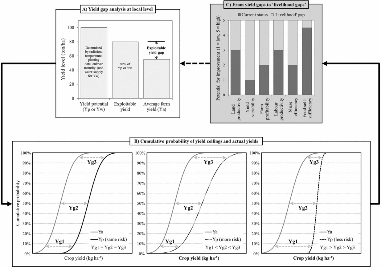
Yield gap analysis at local level needs to go beyond the traditional mean difference between a yield ceiling (e.g., potential yield, Yp, or water-limited yield, Yw) and average farmers’ yields (Ya) in two different aspects. First, it should acknowledge the existence of variability in yield ceilings and Ya by analysing these yield levels in terms of yield distributions instead of single point estimates. Second, yield gaps should be contextualised as one dimension among many within wider livelihood preoccupations. Our focus is to widen the current yield gap approach and raise awareness of the effective contribution of farming to rural livelihoods. Further, we narrow down the approach of van Oort et al. (Reference van Oort, Saito, Dieng, Grassini, Cassman and van Ittersum2016) and illustrate how yield gaps can be used for R&D prioritisation at farm(ing) system level.
In agronomy, yield gaps are used to understand the relative contribution of growth-defining, -limiting and -reducing factors to Ya (van Ittersum and Rabbinge, Reference van Ittersum and Rabbinge1997; Janssen et al., Reference Janssen, Guiking, van der Eijk, Smaling, Wolf and van Reuler1990; French and Schultz, Reference French and Schultz1984; Herdt and Mandac, Reference Herdt and Mandac1981). However, this original purpose has been largely over-simplified in many recent studies (e.g., Kassie et al., Reference Kassie, Ittersum, Hengsdijk, Asseng, Wolf and Roetter2014; Angulo et al., Reference Angulo, Becker and Wassmann2012; Hochman et al., Reference Hochman, Gobbett, Holzworth, McClelland, van Rees, Marinoni, Garcia and Horan2012; Meng et al., Reference Meng, Hou, Wu, Chen, Cui and Zhang2012; Boling et al., Reference Boling, Tuong, van Keulen, Bouman, Suganda and Spiertz2010; Licker et al., Reference Licker, Johnston, Foley, Barford, Kucharik, Monfreda and Ramankutty2010; Lobell et al., Reference Lobell, Cassman and Field2009; Bhatia et al., Reference Bhatia, Singh, Wani, Chauhan, Rao, Mishra and Srinivas2008) which reduce it to the difference between Yp (or Yw) and Ya (Figure 1 A). On the one hand, the simplicity of calculating yield gaps has made this a powerful framing device for justifying policy interventions (Sumberg, Reference Sumberg2012). But on the other hand, the concept is highly problematic, not least because of its flexibility in terms of the yield ceilings considered (examples for rice can be found in Stuart et al., Reference Stuart, Pame, Silva, Dikitanan, Rutsaert, Malabayabas, Lampayan, Radanielson and Singleton2016).
Conceptual framework to integrate yield gap analysis within development-oriented agronomy. (A) Standard yield gap analysis relying on the difference between yield ceilings (Yp or Yw) and actual yields (Ya), e.g., van Ittersum et al. (Reference van Ittersum, Cassman, Grassini, Wolf, Tittonell and Hochman2013) and Lobell et al. (Reference Lobell, Cassman and Field2009). (B) Yield gap analysis based on hypothetical probability distributions of Yp and Ya with differing levels of risk (same, greater or lower than the risk of Ya). (C) Integrated assessment of farm level indicators to identify ‘livelihood gaps’. White boxes depict the ‘farming’ domain in which yield gaps are assessed and the light grey box depicts the livelihood domain in which on-farm and off-farm activities are considered jointly. Arrows illustrate the flow between methodologies required to assess the importance of yield gaps for rural livelihoods.

Yield ceilings and Ya are not single estimates but can be represented by probability curves of varying likelihood (cf. Vanlauwe et al., Reference Vanlauwe, Coe and Giller2016; Beddow et al., Reference Beddow, Hurley, Pardey and Alston2015). In practical terms, farmers hoping to attain the yield ceiling would be interested not only in the maximum production possible but also the risks associated with it: how large is the variance associated with the reported ceiling and are the probability curves normally distributed or skewed. Figure 1 B shows a normally distributed probability curve for a hypothetical set of Ya and Yp. The Ya curve for a given cultivar in a given season is related to factors like planting dates and densities, soil water and nutrient regimes, pest and weed pressures, as well as frequency and timing of weeding operations. The standard yield gap calculation (cf. Figure 1 A) is shown in Figure 1 B as the difference between the median value of Yp and the median value of Ya (Yg2 in each case). This rightward shift corresponds to the treatment effect of eliminating all pertinent limiting factors (cf. Vanlauwe et al., Reference Vanlauwe, Coe and Giller2016).
If the yield ceiling has the same variance as existing practices, the yield ceiling and Ya curves would be parallel to each other and the yield gap would be a constant for all farmers and conditions (Yg1 = Yg2 = Yg3). However, if the yield ceiling has its own variance and level of risk, the yield gap would no longer be a constant. In this case, the difference between the mean values of the yield ceiling and Ya would not be constant for all farms or conditions. Two scenarios present themselves: the yield ceiling could be associated either with more risk or with less risk than is found in the Ya probability curve’s variance. In situations where the yield ceiling is associated with higher levels of risk, the yield gap would be greater than the difference between the median values of the yield ceiling and Ya for the high end of the production curves (Yg3>Yg2), and less than that difference for the low end of the production curve (Yg1<Yg2). However, if researcher-managed conditions eliminated many of the risks associated with on-farm practice (i.e., by limiting biotic and abiotic stresses) and had less risk than the Ya probability curve, we would see the reported yield gap based on the mean values of yield ceiling and Ya under-estimating the yield gap for the lower half of the Ya curve (Yg1>Yg2), while over-estimating it for the upper half of the farms and conditions (Yg3<Yg2).
The relevance of the yield gap for farmers further depends on the overall contribution of agriculture for their livelihoods (Figure 1 C). Farming is not only about biophysical and technical issues (e.g., land productivity and resource use efficiency), but includes other livelihood dimensions as well (e.g., food security, economic viability and drudgery). Identifying opportunities to close yield gaps in farmers’ fields require a diagnosis of a set of indicators as well as knowledge about the importance of off-farm income, the proportion of hired labour to total labour and input-output price ratios, among other issues. Moreover, narrowing yield gaps and increasing resource use efficiency may come at the expense of labour productivity and gross margin. This suggests that agronomy per se cannot eliminate the ‘livelihood gap’ because of possible trade-offs between different livelihood dimensions.
Finally, the identification and adoption of appropriate innovations which respond to the livelihood concerns lead to a new set of yield ceilings, and yield gaps (van Dijk et al., Reference van Dijk, Morley, Jongeneel, van Ittersum, Reidsma and Ruben2017; de Koeijer et al., Reference de Koeijer, Wossink, van Ittersum, Struik and Renkema1999), which are more closely matched to farmers’ personal conditions. In other words, efforts should be made to identify interventions necessary for closing the yield gap component(s) of the livelihood gap.
MAIZE-BASED FARMING SYSTEMS IN WESTERN KENYA
Establishing yield gaps for maize in Kenya
Actual yields (Ya)
Kenya’s maize breeding programme began in Kitale, in the high potential, western highlands, to close the gap between on-station and on-farm conditions. Even then, its first plant breeder, A.Y. Allan bemoaned the lack of reliable on-farm yield data (Allan, Reference Allan1971). He noted measurement as costly and difficult, the widely differing husbandry practices, and the fact that farmers did not accurately know the size of their fields and/or the amounts of maize produced. This knowledge gap was made evident when Allan’s ‘deliberate attempt (on-station) to approximate “poor” husbandry. . . yielded almost 50 percent more (1.97 Mg ha−1) than the estimated average on-farm yield (1.35 Mg ha−1)’ (Gerhart, Reference Gerhart1975). This attempt at duplicating on-farm practice in 26 factorial trials had set six factors sub-optimally (time of planting, plant population, type of seed, standard of weeding, and use of nitrogen and phosphorous), and speaks to the challenge of understanding the full extent of the constraints on maize productivity under farmers’ conditions.
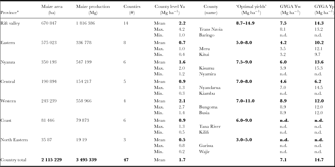
Table 1 shows maize Ya in Kenya for 2014, disaggregated by province and county, compared to various yield ceilings. Even in the most productive parts of the country (Rift Valley, Western and Nyanza provinces), Ya values (whether provincial averages or the Ya from the highest yielding county in each province) remain well below Yp and Yw calculated by GYGA for each province. Although these are the best and most comprehensive Ya data from the government of Kenya, many authors note large discrepancies between official yield statistics and independent yield measurements in African countries (Tittonell and Giller, Reference Tittonell and Giller2013; Wairegi et al., Reference Wairegi, van Asten, Tenywa and Bekunda2010). And there are important errors to consider in the Kenyan case. Not all maize is marketed in Kenya as much of it is consumed by subsistence producers or traded informally, so official Ya statistics are modelled estimates based on measuring the amounts purchased by the National Cereals and Produce Board (NCPB) and sampling within selected counties (GoK, 2015). Due to resource constraints, this sampling cannot be done every year or in every jurisdiction (Hassan et al., Reference Hassan, Onyango and Rutto1998b; Kibaara et al., Reference Kibaara, Ariga, Olwande and Jayne2008). Errors can arise from the lack of consistent crop-cutting, area estimation on irregular fields (Jaetzold et al., Reference Jaetzold, Schmidt, Hornetz and Shisanya2009), and the lack of controls on moisture content at the time of weighing (Grassini et al., Reference Grassini, van Bussel, Wart, Wolf, Claessens, Yang, Boogaard, de Groot, van Ittersum and Cassman2015).
Regional distribution of county-level 2014 maize actual yields (Ya) in Kenya versus yield ceilings (Yw and Yp). Provincial and county Ya and areas (GoK, 2015); optimal yields are the yield ceilings reported for the varieties best suited to each province from (Kang’ethe, Reference Kang’ethe2011); Yw and Yp are the reported averages based on 14 years of data 1998–2011 from GYGA. ‘*’: Provinces were abolished as administrative units in 2010 but remain a useful way to categorise the 47 counties that were created to take their place.

Data quality both for yield ceilings and Ya is highest for the most productive parts of the country. This is logical given the economic and policy incentive to have denser data coverage in these zones, but devotes significant national resources to gathering data in areas where farmers’ yields are already approaching Yw. Primary data are much sparser, and remote sensing is used instead to model productivity, in the more marginal maize growing regions where the yield gap is greatest (e.g., semi-arid Eastern Kenya; Grace et al., Reference Grace, Husak and Bogle2014) or where the economic marginal rate of return for narrowing the yield gap would be greatest (Hassan et al., Reference Hassan, Murithi and Kamau1998a).
Yield ceilings (Yw and Yp)
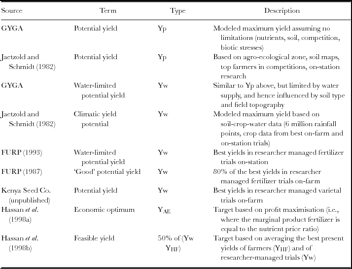
Table 2 illustrates the most commonly used yield ceilings in yield gap estimations in Kenya. Many are variants of Yw either from researcher-managed conditions on-station or on-farm, which reduce all biophysical limitations except moisture (irrigation is not widely available in Kenya, especially in smallholder conditions). As a result, models rely heavily on the quality of input rainfall and soil moisture data (Jaetzold and Schmidt, Reference Jaetzold and Schmidt1982; van Wart et al., Reference van Wart, van Bussel, Wolf, Licker, Grassini, Nelson, Boogaard, Gerber, Mueller, Claessens, van Ittersum and Cassman2013), while Yw based on empirical data (the best yields under managed conditions) show considerable inter-annual and inter-seasonal variation (Hassan et al., Reference Hassan, Murithi and Kamau1998a; FURP, 1993; Rojas, Reference Rojas2007; Smaling and Janssen, Reference Smaling and Janssen1993).
Examples of yield ceilings against which actual on-farm yields in Kenya have been compared. Terms are reported as in the original reference.

Field measures
Initial on-station research in the 1960s and 1970s established the importance of early planting, high plant densities, and high standards of weeding (Allan, Reference Allan1971). Subsequent research has explored the crop response to inputs especially N and P (FURP, 1986; Njoroge et al., Reference Njoroge, Mugo and Laboso1995). As a result, all treatments in more recent trials share many elements of crop husbandry that are not necessarily desirable or suitable for smallholder farmers. Although most farmers intercrop their maize with legumes, the vast majority of research trials consider sole stands of maize. For example, the National Performance Trials (NPTs) use comparatively few factorial treatments (usually only N or P combinations), with 1–4 replicates on 5 m × 5 m plots, meaning typically 24–48 maize plants harvested from the inner 4 out of 6 rows planted (Njoroge et al., Reference Njoroge, Mugo and Laboso1995). Trial sites are chosen to be ‘representative of the target area’ yet, unlike many of the farms that they are supposed to represent, should also be ‘as uniform as possible in terms of slopes, soil types and previous cropping history’ and ‘preferably not planted with maize the previous season’ (Njoroge et al., Reference Njoroge, Mugo and Laboso1995).
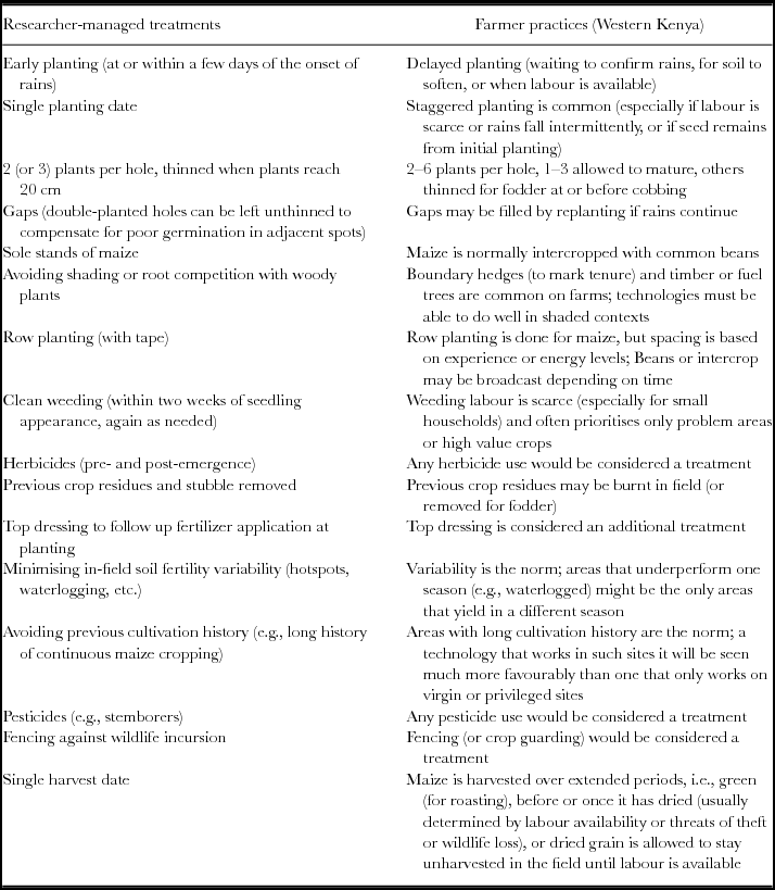
Although this configuration follows international agronomic norms, and allows for robust statistical testing while maximising the use of scarce research station land, this design erases a number of factors actually found in farmers’ fields, or introduces design elements that would themselves be considered treatments. Participatory research in six communities of western Kenya between 2001 and 2008 worked to build a shared understanding of soil fertility and crop husbandry under smallholder conditions (Ramisch et al., Reference Ramisch, Misiko, Ekise and Mukalama2006). Focus group discussions and individual interviews with smallholder farmers and scientists in the early stages of the project helped identify discrepancies in the knowledge and attitudes of the different groups.
Table 3 summarises findings from 2002 and 2003 about how researchers and smallholder farmers each defined ‘good husbandry’. These are not trivial differences. Many of the high yielding practices defined as good husbandry by researchers, and which are used as the basis for determining yield ceilings under researcher-managed trials, were seen as too risky or simply unwise by smallholder farmers. For example, planting on a single date, planting relatively few seeds per hole, and planting maize without an intercrop (especially a legume) each appeared to many respondents as risky gambles that did not offer the households any alternatives if the promised maize yield improvements failed to materialize. Farmers also discounted the value of selection criteria such as minimising in-field soil variability, competition with woody plants, and avoiding histories of continuous maize cultivation, since technologies were deemed more impressive if they could succeed in more typical and challenging contexts. Finally, standard measures taken by researchers to protect trial sites and treatments from interference or loss (fencing, herbicides, pesticides, and clean weeding) were each considered treatments in their own right, and therefore as interesting as potential innovations as the varietal testing or soil fertility management treatments ostensibly being tested (Ramisch, Reference Ramisch2011).
Husbandry on researcher-managed sites that are taken as ‘best practices’ versus equivalent on-farm practices in western Kenya. Source: Focus group discussions conducted with farmers and scientists in the six study communities of western Kenya (2002–2003; cf. Ramisch, Reference Ramisch2014).

Farmers called special attention to early planting as a problematic practice even while they acknowledged its favourable impact on yields if rains fell reliably. The key concern is a social one: farmers with maize ripening early in the hungry season between weeding and harvest face considerable social pressure to share this abundance with less fortunate kin or neighbours (Ramisch, Reference Ramisch2016). The ability to put in place practices to reach a supposed yield ceiling may thus be compromised by a farmer’s unwillingness to incur the social or moral consequences. Bunei et al. (Reference Bunei, Rono and Chessa2013) confirmed that fear of crop theft indeed drives some farmers in the Rift Valley to avoid planting early ripening varieties of maize or beans, or to not invest in soil fertility management that would otherwise increase their maize yields.
Maize yield distributions in western Kenya
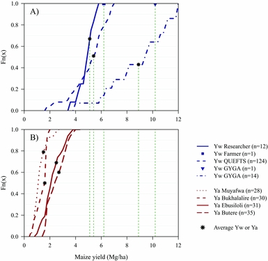
One way to accommodate these differences in perception is to acknowledge the range of probabilities of outcomes for yield ceilings and actual farmers’ yields. Researcher- and farmer-managed maize trials from four sites in western Kenya are presented in Figure 2 to illustrate the challenge of moving from yield gaps (Figure 1 A and B) to ‘livelihood gaps’ (Figure 1 C).
Maize yield gaps during the 2007 long rains based on A) five different variants of Yw and B) cumulative probability curves of Ya in four western Kenyan sites. The asterisks (*) represent the mean value for each curve. Ya as well as Yw_farmer, Yw_researcher and Yw_QUEFTS are all unpublished project data. See text for further information regarding data sources.
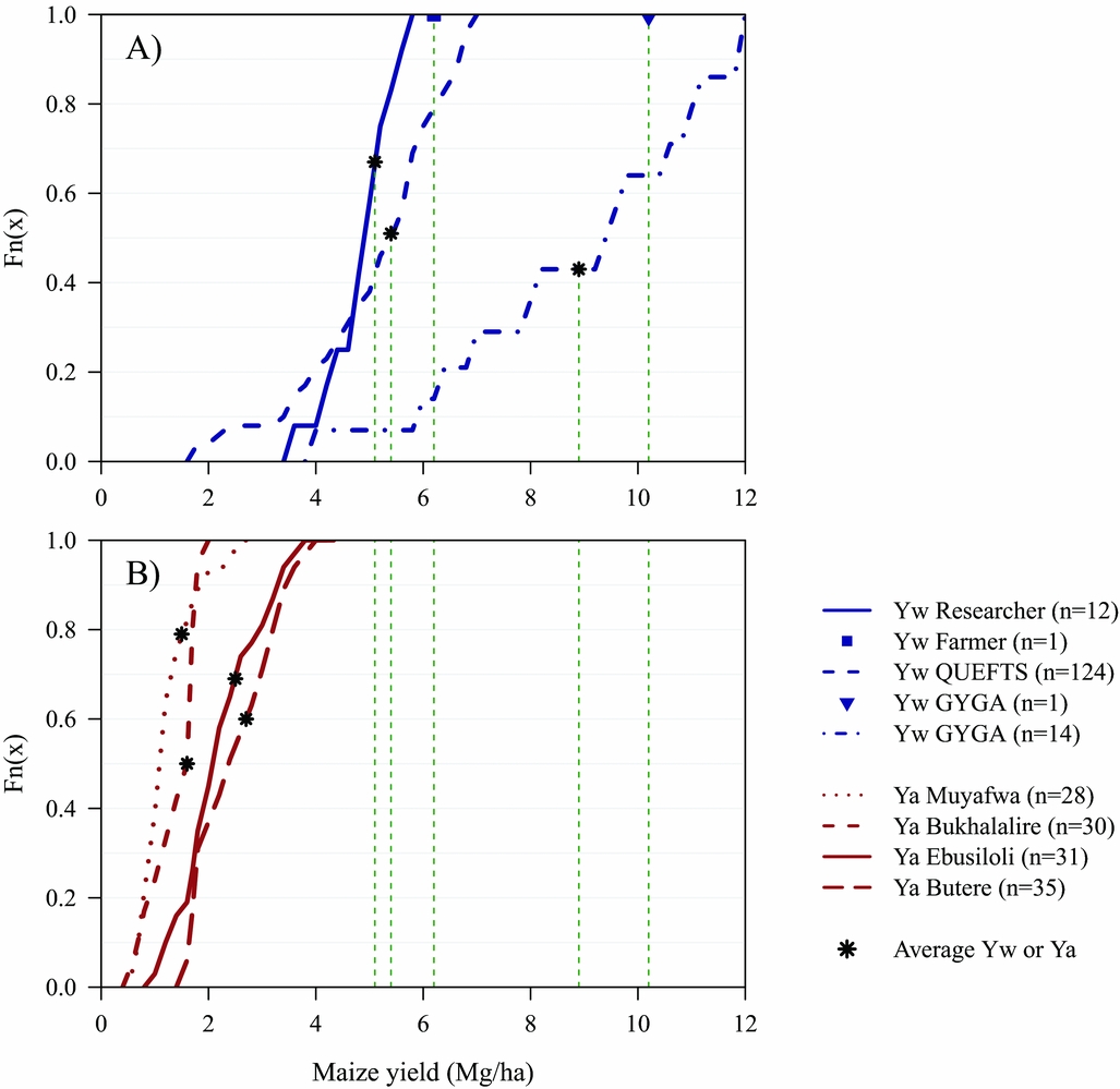
Figure 2 illustrates the challenges of a yield gap analysis in western Kenya once we use probability curves for both Ya and Yw. In the lower panel (Figure 2 B), four cumulative probability curves represent the range of farmer-managed Ya harvested in the long rains of 2007 in four communities (Muyafwa, Bukhalalire, Ebusiloli and Butere; see Supplementary Figure S1). Households differed substantially in their socio-economic and soil fertility status in ways which were unequally distributed through the sample, making it important to consider the cumulative distribution of Ya and not just the mean. The upper panel (Figure 2 A) shows five different but potentially plausible yield ceilings:
1. The cumulative probability curve for the twelve top-yielding researcher-managed plots in the same communities in the same season (Yw_researcher), which averaged 5.1 Mg ha−1. Each study site had three researcher-managed experiments that were used for demonstrations. The highest yielding plots in each of these experiments (typically a “best practice” management of nutrients and crop husbandry), could therefore be considered by farmers as the upper benchmark of possible production under local conditions.
2. The single highest yield recorded on a farmer-managed plot (Yw_farmer) in any of the communities over the project’s lifetime (2001–2008; 6.0 Mg ha−1). Many farmers (and the research team) took note of the fact that the best recorded yield by a farmer was higher than that seen on the researchers’ own “best practice” plots (at least in 2007). Other participating farmers found it easy to accept this yield as the most logical target as the “maximum” production possible under local conditions.
3. The Yw curve for all 154 farmer-managed plots simulated for non-limiting nutrient conditions using QUEFTS (Smaling and Janssen, Reference Smaling and Janssen1993, as applied by Tittonell et al., Reference Tittonell, Vanlauwe, Corbeels and Giller2008; Yw_QUEFTS), which averaged 5.4 Mg ha−1. Because soil fertility is heterogeneous in these sites (Vanlauwe et al., Reference Vanlauwe, Tittonell and Mukalama2007), the QUEFTS model was used to predict crop yields based on actual soil fertility measures and assumptions about the recovery fractions of applied nutrients. Although the model does not consider other husbandry factors, it does assess the yields possible if nutrients were non-limiting.
4. The Yw point simulated by the Global Yield Gap Atlas for these sites, which is shown in Supplementary Figure S1 for the climate zone to which all four sites belong (Yw_GYGA, 10.2 Mg ha−1). The model simulates the performance of recently-released, high yield cultivars grown in single stands, and is calibrated on the basis of local soil properties, long-term (>10 years) daily weather data, and crop management data (sowing date or sowing rule and plant population density) as per http://www.yieldgap.org/web/guest/methods-model-calibration.
5. The Yw curve generated from the 14 years of experimental data collected by the Global Yield Gap Atlas for the Kakamega weather station, which averaged 8.9 Mg ha−1 (Yw_GYGA14). Unlike the modelled data (Yw_GYGA), this value might be easier for farmers to relate to, since it was derived from actual yields obtained under optimal, researcher-managed conditions.
Yield gaps for any of the four site’s Ya curves represented in Figure 2 B could legitimately be calculated against each of the five yield ceilings shown in Figure 2 A. The dotted lines bridging the upper and lower panels of Figure 2 link to either the point estimate or the mean value of the probability curve for each of the five Yw curves or estimates, leading to five different sets of possible ceilings. The highest yield ceiling (the GYGA point estimate of 10.2 Mg ha−1) is twice the value of the lowest ceiling, the average of the top-yielding researcher-managed plots (5.1 Mg ha−1). Including all fourteen years of available data moderates the GYGA target somewhat, to 8.9 Mg ha−1 but precipitation at the Kakamega weather station on which Yw_GYGA14 is based (1971 mm yr−1) is at the more favourable end of the precipitation range recorded in the study sites (1270–2000 mm yr−1, Ramisch et al., Reference Ramisch, Misiko, Ekise and Mukalama2006). Beyond the diversity of possible Yw targets, yield gap calculations based on the averages or point estimates of Yw would tell us little about the probabilities of attaining the maximal yields for any of the given farms within the sample. Even the QUEFTS calculations, which drew upon the farmers’ own local conditions, generated yield gaps between 0.7 and 6.5 Mg ha−1 but do not convey the probabilities related to closing those gaps. Yet, this is a crucial consideration for farmers deciding whether or how to narrow any perceived gap.
The Kenyan case study suggests that neither Ya nor Yw data can easily be taken at face value, since the calculation of both is based on sets of socially-determined decisions about what to accept and what to exclude. By the same token, the significance of the presence (and scale) of a gap between Yw and Ya needs to be fit within a context of the probabilities of attaining a given yield as well as the livelihood significance of what closing (or failing to close) that gap would mean.
RICE FARMING SYSTEMS IN CENTRAL LUZON, PHILIPPINES
Context and household survey
Rice is the staple food in the Philippines. The average per capita rice consumption in the country has increased from ca. 100 kg capita−1 year−1 in the 1980s up to ca. 130 kg capita−1 year−1 in the 2000s (USDA and FAOSTAT databases). Despite the rapid development of the off-farm sector (e.g., construction, industry, transport, services and remittances) over the past decades, rice farming remains an important activity in Central Luzon contributing up to 25% of the total household income (Takahashi and Otsuka, Reference Takahashi and Otsuka2009) and being an important source of employment to many (landless) peasants (Kerkvliet, Reference Kerkvliet1990). Double rice cropping systems are common in this region, with a wet season (WS) crop between June/July and September/October and a dry season (DS) crop between December/January and March/April. Historically, the traditional season for rice farming was the WS but the increasing investments in irrigation facilities and the release of short cycle varieties made possible the cultivation of a subsequent rice crop in the DS (Cassman and Pingali, Reference Cassman and Pingali1995).
The Central Luzon Loop Survey is a historical household survey which has been collected by the International Rice Research Institute (IRRI) every 4 to 5 years since 1966 up to now. The survey has been conducted to monitor changes over time in crop management and household characteristics in the rice-based farming systems of Central Luzon (Silva et al., Reference Silva, Reidsma, Velasco, Laborte and van Ittersum2018; Moya et al., Reference Moya, Kajisa, Barker, Mohanty, Gascon and Valentin2015). On average, 103 rice farming households were interviewed in the WS and 59 in the DS. Most households were interviewed in the WS and DS of the same crop year but the sample size is lower in the DS because of water-related constraints or cultivation of other crops.
Rice yields and yield gaps
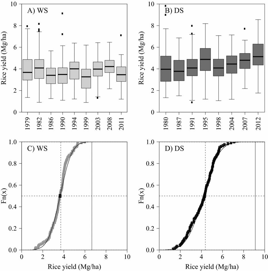
Rice yield gaps (Yp–Ya) in Central Luzon were on average 3.2 Mg ha−1 in the WS and 4.8 Mg ha−1 in the DS during the period 1979–2012 (Laborte et al., Reference Laborte, de Bie, Smaling, Moya, Boling and van Ittersum2012; Silva et al., Reference Silva, Reidsma, Velasco, Laborte and van Ittersum2018). There was no significant increase in Ya during the WS, which remained ca. 3.8. Mg ha−1 over the period analysed (Figure 3 A). Stagnation of Ya in the WS may be attributed to risk of lodging due to typhoons at high N application levels (Lampayan et al., Reference Lampayan, Bouman, de Dios, Espiritu, Soriano, Lactaoen, Faronilo and Thant2010; Lansigan et al., Reference Lansigan, de los Santos and Coladilla2000; Loevinsohn et al., Reference Loevinsohn, Bandong and Alviola1993). Conversely, there was a significant increase in Ya during the DS over the period 1979–2012 from ca. 4.0 Mg ha−1 in 1980 up to 5.2 Mg ha−1 in 2012 (Figure 3 B). Typhoons do not occur during this season, which reduces climatic risks considerably, and provides more favourable growing conditions for rice, as indicated by the higher Yp compared to the WS. In addition to increases in Ya, there was also a significant increase of N application during the DS. Modern varieties were readily and widely adopted over the past half-century in Central Luzon, which also contributed to increases in Ya.
Rice yields and yield gaps based on cumulative probability curves of Ya in Central Luzon, Philippines. Data for the WS and DS are presented on the left (A and C) and right (B and D), respectively. In C) and D), Ya values reported refer to averages across years for each farm and horizontal dashed lines show the 50% probability, vertical dashed lines shows the median of Ya, vertical solid lines show the simulated Yp averaged over the WS and DS periods (6.7 and 9.2 Mg ha−1, respectively; see Silva et al., Reference Silva, Reidsma, Laborte and van Ittersum2017 for further details) and the normal distribution is shown as the solid line.

The distribution observed for rice yields approximated a normal distribution in both seasons (Figure 3 C and D). The median Ya was 3.7 Mg ha−1 in WS and 4.4 Mg ha−1 in DS. However, there was a large variability around these values with a minimum of 1.3 and 1.4 Mg ha−1 and a maximum of 6.1 and 7.2 Mg ha−1 in the WS and DS, respectively. The highest Ya values were close to Yp in the WS (minimum difference of 0.6 Mg ha−1) but not in the DS (minimum difference of 2.0 Mg ha−1). Rice yield gaps were as large as 5.3 Mg ha−1 and as small as 0.6 Mg ha−1 in WS and as large as 7.7 Mg ha−1 and as small as 2.0 Mg ha−1 in DS (see horizontal distance between Yp and Ya in Figure 3 C and D).
Moving toward ‘livelihood gaps’
Yield gaps per se are not very informative about the possibility to improve livelihoods of rural households (Figure 1 C). For this purpose, they need to be analysed in relation to other indicators of farm performance capturing the broader livelihood aspects within which farming takes place. The farm level indicators analysed in this paper were labour productivity (kg ld−1), gross margin (Philippine Peso, PhP, ha−1) and rice self-sufficiency at household level (%). Methodological details about the estimation of these indicators are provided as Supplementary Material.
Labour productivity
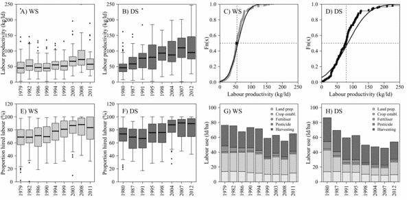
Labour productivity increased over time in both WS and DS (Figure 4 A and 4 B). The increase in this indicator was particularly evident in the DS, from about 51 kg ld−1 in 1980 up to about 120 kg ld−1, in 2012. This increase can be explained by a combination of increases in Ya (Figure 3 B) and adoption of labour-saving technologies such as direct-seeding, small tractors, threshers and herbicides (Moya et al., Reference Moya, Kajisa, Barker, Mohanty, Gascon and Valentin2015). The median labour productivity observed during the WS and DS was about 55 and 79 kg ld−1 (Figure 4 C and D), respectively, and the variation observed in this indicator approximated a normal distribution in the WS, but not as much in the DS.
Labour productivity (A–D) and dynamics (E–H) in rice-based farming systems in Central Luzon, Philippines. In (C) and (D), labour productivity values reported refer to averages across years for each farm and horizontal dashed lines show the 50% probability, vertical dashed lines shows the median of gross margin, vertical solid lines show the gross margin equal to zero and the normal distribution is shown as the solid line.

There was a sharp increase in the proportion of hired labour over time up to an average of ca. 82% of the total labour used for rice farming in 2011/2012 (Figure 4 E and F). The replacement of family by hired labour was particularly evident after the year 2000. This trend suggests that the importance of rice farming as a landowning household’s primary occupation declined over time. The decline in hired labour between 1979 and 2000, and its increase afterwards, was associated with land preparation and crop establishment practices used by farmers. For example, labour use for crop establishment declined in the 1980s and 1990s and slightly increased again in the 2000s (particularly in the DS) because of the adoption of direct seeding during the 1990s and the re-adoption of transplanting after the 2000s (Figure 4 G and H), respectively. Labour use for land preparation and crop management slightly decreased over time mostly due to the adoption of small tractors and herbicides, respectively.
Gross margin
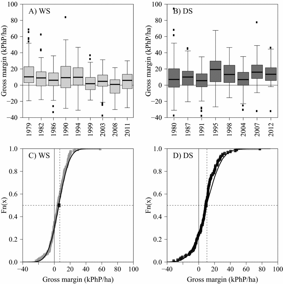
There was a significant decline in gross margin from rice farming over time during the WS (Figure 5 A) while no trend was observed in the DS (Figure 5 B). In the WS, this can be explained by a slight decline in revenues, attributed to yield stagnation and a slight decline in paddy prices (Silva et al., Reference Silva, Reidsma, Velasco, Laborte and van Ittersum2018), and by an increasing of production costs due to greater use of hired labour and material inputs (data not shown). The negative gross margin of WS rice observed for many households shows rice farming is not economically rewarding during this season especially given current amounts of hired labour and high labour wages in the region (Moya et al., Reference Moya, Dawe, Pabale, Tiongco, Chien, Devarajan, Djatiharti, Lai, Niyomvit, Ping, Redondo, Wardana, Dobermann and Witt2004). It is worth noting that the median gross margin in the 2008 WS was even negative. By contrast, revenues and production costs during the DS increased over time. The increase in revenues was explained by increases in Ya (Figure 3 B), since paddy prices slightly declined. Similarly to the WS, increasing production costs were explained by greater use of hired labour and, to a lesser extent, material inputs (e.g., real prices of N declined between the late 1960s and early 2000s, after which there was a sharp increase).
Gross margin of rice-based farming systems in Central Luzon, Philippines: (A) and (B) trends over time, (C) and (D) cumulative probabilities. In (C) and (D), gross margin values reported refer to averages across years for each farm and horizontal dashed lines show the 50% probability, vertical dashed lines shows the median of gross margin, vertical solid lines show the gross margin equal to zero and the normal distribution is shown as the solid line.

The median gross margin from WS rice and DS rice was 5305 and 9525 PhP ha−1, respectively, and the distribution observed in this indicator approximated a normal distribution in both seasons (Figure 5 C and D). The threshold probability for positive gross margins was ca. 30% in the WS and ca. 20% in the DS. The maximum gross margin observed was far greater than the minimum gross margin in absolute terms. However, the low median and high probability of negative gross margin in the WS question again the importance of rice farming as a source of income for many households in this season. For instance, in 1979 WS and 1980 DS ca. 25% of the households had negative gross margin from rice farming as compared to 2011 WS and 2012 DS in which 14% and 5% of the households had negative gross margin, respectively. The largest number of households with negative gross margin (ca. 48%) was recorded in 2008 WS. The importance of positive gross margin for each household is likely to increase with decreasing importance of off-farm income. Negative gross margin over consecutive seasons for households not depending on off-farm income may limit investments in, e.g., education in the short-term and lead to migration to urban areas in search of non-agricultural employment in the long-term.
Rice self-sufficiency
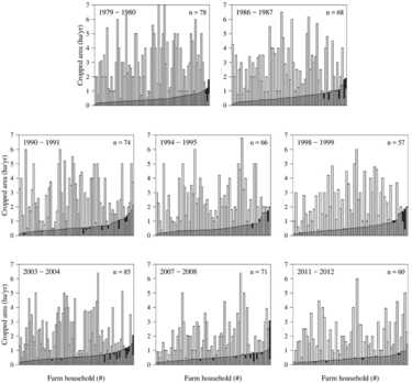
During the period 1979–2012, less than 15% of the households did not meet their yearly rice requirements (Figure 6). This indicates that (1) the majority of households in Central Luzon achieved rice self-sufficiency with current rice yields, cultivated area and consumption requirements (i.e., household size and per capita rice consumption) and (2) most households have a considerable amount of land surplus to produce rice for the market. Indeed, Central Luzon is known to be the rice bowl of the Philippines, and particularly of Metro Manila.
Yearly land requirements for rice self-sufficiency (ha, medium grey), land surplus (ha, light grey) and land deficit (ha, dark grey) between 1979 and 2012 in Central Luzon, Philippines. Cropped area refers to the sum of the area of each field cultivated by an individual household in both WS and DS. Each bar represents the total cropped area by an individual household in one year.

The land required for rice self-sufficiency at household level remained constant over time with an average of ca. 0.5 ha per household, and ranging between ca. 0.4 and 0.6 ha per household in 2011/2012 and 1986/1987, respectively. The additional amount of land required to achieve rice self-sufficiency at household level (i.e., land deficit) was also rather constant over time and its negligible magnitude confirms that most households were able to meet their domestic consumption needs. The average land surplus, i.e., the actual amount of land cultivated not needed for rice self-sufficiency at household level, declined significantly over time from ca. 2.7 ha in 1979/1980 to 2.1 ha in 2011/2012. The significant decline in land surplus can be attributed to increased rice demand and decreased rice supply over time. The latter occurred due to greater per capita consumption and adult:child ratio, while the former was due to a slight, but significant, decline in rice cropped area possibly explained by the cultivation of other crops and/or land conversion to non-agricultural uses.
Rice and rural livelihoods
The data from our sample shows large rice yield gaps persist in Central Luzon, particularly during the DS (Figure 3), indicating there is considerable scope to increase rice production in this farming system (Laborte et al., Reference Laborte, de Bie, Smaling, Moya, Boling and van Ittersum2012; Silva et al., Reference Silva, Reidsma, Laborte and van Ittersum2017). However, as with the Kenyan examples, the benefits from narrowing such yield gaps depend on whether or not increased production (1) is associated with similar or reduced risks compared to the current situation, (2) translates into significantly greater returns to land and/or labour and, (3) is required to meet self-sufficiency needs at household level.
Climatic risk is a very important aspect in Central Luzon as intensification of N use increases the probability of lodging during the WS due to frequent incidence of typhoons in this time of the year (Lampayan et al., Reference Lampayan, Bouman, de Dios, Espiritu, Soriano, Lactaoen, Faronilo and Thant2010; Lansigan et al., Reference Lansigan, de los Santos and Coladilla2000; Loevinsohn et al., Reference Loevinsohn, Bandong and Alviola1993). An example of the impact of typhoon damage on rice stands under field conditions is depicted in Supplementary Figure S2. In this on-station trial, the treatment replicating N application rates used by farmers in the region (i.e., 60 kg N ha−1) did not suffer from lodging after typhoon while the treatment aiming to achieve Yp (i.e., 180 kg N ha−1) resulted in complete crop failure. In these extreme situations, farmers would most likely find little incentive to increase N application rates beyond levels currently used.
In addition to the biophysical risks associated with higher yields and more intensive management practices, it is important to consider farmers’ financial and food security incentives to narrow the yield gap. Figure 6 demonstrates that actual rice yields and current farm sizes have been able to satisfy the caloric need of most households between 1979 and 2012. Rice self-sufficiency at household level indicates that the main incentive for narrowing rice yield gaps would then be for commercial, rather than domestic consumption, purposes. Formal research might indeed encourage such a shift in production orientation, but in a context where narrowing the yield gap goes in tandem with high input costs (especially hired labour), marginal additional income from selling rice (Figure 5) and increased risk of more intensive input use in the WS (e.g., Supplementary Figure S2).
The low gross margin of rice farming has been compensated by an increase in non-agricultural sources of income such as off-farm employment and remittances (Estudillo and Otsuka, Reference Estudillo and Otsuka1999; Moya et al., Reference Moya, Kajisa, Barker, Mohanty, Gascon and Valentin2015; Takahashi and Otsuka, Reference Takahashi and Otsuka2009). The high labour wages for on-farm work observed in Central Luzon compared to other rice bowls in Southeast Asia (Moya et al., Reference Moya, Dawe, Pabale, Tiongco, Chien, Devarajan, Djatiharti, Lai, Niyomvit, Ping, Redondo, Wardana, Dobermann and Witt2004) did not discourage most households from replacing family by hired labour over the past half-century (Figure 4 E and F). This indicates that opportunity costs for family labour in the non-agricultural sector are also high in the region as otherwise it would not be economically rational to depend so much on hired labour for rice production, which accounts for more than 50% of the production costs. In this context, any efforts to narrow the yield gap would most likely require even heavier reliance on hiring permanent and/or casual labourers for operations like crop establishment and harvesting (Figure 4).
The analysis of rice yield gaps vis-à-vis gross margin, labour productivity and rice self-sufficiency provides insights into the relative importance of rice farming for rural livelihoods in Central Luzon. In addition to the trade-offs between yield gap closure on the one hand and labour productivity and N use efficiency on the other hand (Silva et al., Reference Silva, Reidsma, Velasco, Laborte and van Ittersum2018), it is questionable whether rice production will be intensified in Central Luzon under prevailing conditions given that greater yields are associated with greater risk of crop failure in some periods of the year (Supplementary Figure S2), economic returns to land are marginal (Figure 5) and rice self-sufficiency at household level is not at stake (Figure 6). Observed trends in off-farm income and labour dynamics further confirm the clear preference of most households for more regular, and less labour intensive, sources of income leaving us with the question of who should close which yield gap.
DISCUSSION
The standard yield gap is conceptually simple, and therefore easy to explain to non-specialist policy-makers (e.g., ‘how much more food could our farmers grow?’). This makes it challenging to contest or replace. The two case studies illustrate how moving from yield gaps to ‘livelihood gaps’, and acknowledging the probabilities and risks inherent in narrowing such gaps, are important points to communicate in contexts where agronomy has much to offer but where farming is only one element within a suite of livelihood options.
Incorporating variability into yield gap analysis
Farming systems research can point to multiple successes in both the Kenyan and the Philippines context. The dramatic increase of maize yields observed in Kenya between 1965 and 1980 is widely hailed as a success story for African maize agronomy, which saw the release and widespread adoption of varieties suited to a range of agro-climatic conditions (Smale and Jayne, Reference Smale and Jayne2003). A similar productivity improvement was observed in the Philippines with the development of irrigation facilities and short cycle varieties, which allowed the cultivation of rice in both WS and DS (Cassman and Pingali, Reference Cassman and Pingali1995).
Despite these successes, current yields (Ya) both of maize in Kenya and rice in the Philippines lag behind their full potential. The two case studies demonstrate that by failing to consider variability and risk in both actual, on-farm conditions (Ya) and yield ceilings (Yw or Yp), conventional yield gap analyses only partially explain where and how Ya could be improved. For example, in both contexts experimental evidence shows that increased fertilizer use is associated with greater risk of crop failure. In Kenya, the nationwide Fertilizer Use and Recommendations Project (FURP) trials provided experimental and modelled Yw far above Ya, but the yield increases due to fertilizer use were also often associated with increased yield variability (Roetter and van Keulen, Reference Roetter and van Keulen1997). In the Philippines, greater N use was also associated with greater yield variability due to increased risk of lodging during the WS (e.g., Supplementary Figure S2; Lampayan et al., Reference Lampayan, Bouman, de Dios, Espiritu, Soriano, Lactaoen, Faronilo and Thant2010). Extending the yield frontier should not only offer the promise of higher Ya but should also seek to reduce the risk associated with those improvements, i.e., tightening the distribution of the cumulative probability curves rather than stretching or skewing them.
Field and farm variability is recognized in agronomy through different site-specific approaches (Dobermann et al., Reference Dobermann, Witt, Dawe, Abdulrachman, Gines, Nagarajan, Satawathananont, Son, Tan, Wang, Chien, Thoa, Phung, Stalin, Muthukrishnan, Ravi, Babu, Chatuporn, Sookthongsa, Sun, Fu, Simbahan and Adviento2002; Vanlauwe et al., Reference Vanlauwe, Descheemaeker, Giller, Huising, Merckx, Nziguheba, Wendt and Zingore2015). As data from Central Luzon shows, where a farm lies on the Ya probability curve (Figure 3) is not independent of its placement on labour productivity or gross margin probability curves (Figures 4 and 5). In western Kenya, the FURP trials not only included a range of cropping conditions for maize (sole stands and intercropped), but reported its findings using three different probability thresholds (0.33, 0.50 and 0.66) for purposes of calculating economic benefits. The FURP’s approach should be followed and extended upon. Many of the currently used yield ceilings (Table 2) entail data quality issues relating to upscaling (e.g., GYGA), or assumptions about risk and treatment design that make their claims of biophysical objectivity hard for farmers to accept. For example, Herdt (Reference Herdt1979) found a significant decrease in on-station rice yields when the production objective was switched from yield maximisation to gross margin maximisation and recent efforts have shown similar results for maize in Tanzania (van Dijk et al., Reference van Dijk, Morley, Jongeneel, van Ittersum, Reidsma and Ruben2017). However, even these optimal yields need to be contextualized at farm(ing) systems level to understand how exactly households may benefit from possible yield gains.
Embedding yield gaps into rural livelihoods
Yield gaps that identify where (and by how much) crops and farm(ing) systems can be improved are important guides for technology development, but must also help guide decision-making about which technologies are worthwhile investments. In western Kenya, many farms are smaller than 0.5 ha and can provide 3–7 months of food security (Ramisch, Reference Ramisch2014). To attain a full year’s food supply, the food insecure households would need to increase Ya by a factor of four while avoiding losses (e.g., theft or post-harvest).
Ideally, in an on-farm setting, it would be possible to identify the degree to which a given variable could be improved given specific objectives and resource constraints. Optimisation techniques can be used for the more easily quantified data, which tend to be the biophysical and those economic aspects that engage with the formal sector. However, these methods are more conjectural and ill-suited for qualitative data, or those quantitative data that lack precision or accuracy. Farmers make decisions about how much energy or resources they want to invest in agriculture (let alone in closing yield gaps). However, while decisions to opt out of farming (or to rely on hired rather than family labour) may be rational for many households, better information about how farmers perceive and respond to variability and risk could guide better technology development for those households that decide to persist in the agricultural sector. Such qualitative information would also be helpful to guide those households at the lower end of the Ya or yield ceiling cumulative probability curves to understand the risks, opportunities and trade-offs.
This makes it essential that the real costs and risks associated with attaining yield ceilings are made more explicit. The differing perspectives on what constitutes a ‘treatment’ (Table 3) reveal the frustrations that farmers have with researchers as well as the ways in which researchers perceive and understand the constraints farmers face. As Allan (Reference Allan1971) noted ‘demonstrating differences of 10% in yield is a waste of time in developing countries’, which led him to advocate for a ‘package approach’ that would maximize all possible input factors so that even if one factor had no effect, the overall differences of the new maize-growing system would be ‘very much higher than the average yields [Ya] round about’. This ‘new system’ might persuade some farmers, but without a clearer understanding of all the costs and risks involved in surpassing their local Ya, many farmers might dismiss the package approach as impossible, uneconomic, or irrelevant.
Looking up: Dynamics at national level
Even if individual households are making the appropriate choice (for them) to get out of staple food production, the national food security picture is deteriorating in both Kenya and the Philippines. From a policy standpoint, the yield gap is paired with the costs of imports to meet consumption needs not covered by domestic production (e.g., van Ittersum et al., Reference van Ittersum, van Bussel, Wolf, Grassini, van Wart, Guilpart, Claessens, de Groot, Wiebe, Mason-DCroz, Yang, Boogaard, van Oort, van Loon, Saito, Adimo, Adjei-Nsiah, Agali, Bala, Chikowo, Kaizzi, Kouressy, Makoi, Ouattara, Tesfaye and Cassman2016). Between 1970 and 1991, maize imports represented 2.9% of total annual maize consumption in Kenya, growing to an average of 12% for the period 2000–2010 (Kimani and Gruere, Reference Kimani and Gruere2010). Population increase over this period accounts for some of the increased demand, but the liberalisation of the maize marketing system in the 1990s played a role in making low cost maize available from the neighbouring countries. This discouraged some smallholders from investing resources in higher cost domestic maize production (Nyoro et al., Reference Nyoro, Kirimi and Jayne2004). Most of the maize is grown in the former Rift Valley, Western, and Nyanza Provinces (84%; Table 1) and, other things being equal, the country could meet its consumption needs by closing part of the yield gap in these regions.
National policies in the Philippines have focused on promoting rice self-sufficiency and providing high income to farmers (PDA, 2012) while ensuring affordable prices for consumers (PSA, 2017). However, rice imports in the country accounted for ca. 10% of total rice consumption in 2015 and there has been an increasing import dependency over time (PSA, 2017; particularly from Vietnam and Thailand). The Philippines has been the largest rice importing country in the world (Dawe et al., Reference Dawe, Moya and Casiwan2006) due to unfavourable geography (Dawe, Reference Dawe2006), population growth (FAOSTAT, 2017) and poor irrigation infrastructure (Barker and Levine, Reference Barker and Levine2012). Future perspectives are not very promising given that rice production needs to double, due to population growth, if self-sufficiency is to be achieved by 2050. This seems very improbable given ‘current trends in yield growth, existing production technologies, and prevailing conditions’ (Laborte et al., Reference Laborte, de Bie, Smaling, Moya, Boling and van Ittersum2012). The later include the fact that rice farming is one in many livelihood activities for many households in Central Luzon, the prime rice producing area of the country.
In both countries, it is important that consumers have confidence that the national food system delivers the commodities in sufficient quantity and at affordable prices. Regular maize shortages due to fertilizer price instability, or to extreme events such as the Kenya’s 2008 post-election violence indicate that, even if the Rift Valley could grow all of Kenya’s maize, it is logical for smallholders countrywide to keep growing their own (higher cost) maize ‘just in case’ (Brooks et al., Reference Brooks, Thompson, Odame, Kibaara, Nderitu, Karin and Millstone2009). Similar concerns are observed in the Philippines where rice farm-gate prices (Cabling and Dawe, Reference Cabling and Dawe2006) and consumer rice prices (FAO/FPMA, 2017) are among the highest in Southeast Asia. Rice prices are established by the National Food Authority (NFA), a governmental agency that controls the national rice market in terms of rice imports and acquisition of rice from farmers at support price.
CONCLUSION
The two case studies explored how yield gap analysis can be expanded to consider the variability of yield ceilings and actual yield and to situate the yield gap within a wider livelihood context. Using the ‘livelihood gap’ concept to develop pathways to improved food security needs to acknowledge that farming in many smallholder contexts is one within multiple livelihood activities and it often entails biophysical and/or socio-economic risks as yield gaps are narrowed. Developing a shared understanding of risk and opportunity is crucial, since farmers and researchers often differ in their perceptions and understanding not only of risk but even of what constitutes a ‘treatment’ (Table 3).
Future research and development initiatives at farming systems level aiming at better understanding ‘whose gap counts?’ require an extension of the current yield gap analyses in different ways. Our case studies in Western Kenya and Central Luzon, the Philippines, provide some entry points for future assessments of ‘livelihood gaps’ which can be summarised as follows:
• Yield gap analyses conducted at farming systems level need to acknowledge the temporal and spatial variability of crop yields. In practical terms, this means that yield ceilings and actual yields are better represented by cumulative probability curves rather than by single point estimates such as the mean or the maximal values. Future efforts should thus seek to reduce the yield gap between the water-limited and the actual yield probability curves while ensuring similar or lower risks than found in the current situation.
• Although a measurable yield gap can exist between the yields of researcher- and farmer-managed plots, yield maximisation will rarely be the sole objective of farmers. As with widening our understanding of risk, it is also crucial to broaden our attention to other aspects of smallholder farming systems in the future, and their trade-off with land productivity, such as their economic viability and labour productivity. This should be done with the help of different indicators (as illustrated in our case by crop yield, labour productivity, gross margin and self-sufficiency) selected on a case study basis.
• Crop production is central to most smallholder farming systems, but food and livelihood security is also linked to other livelihood strategies. In our case studies, off-farm income is a crucial pillar in the livelihoods of rural households, but in other settings different strategies of natural resource management may be just as important. Engaging with this broader livelihood diversity is thus needed to define more realistic and attainable yield gaps.
Finally, moving from yield gaps to ‘livelihood gaps’ will require more careful consideration of data needs. For instance, the communities studied in western Kenya correspond to four different production contexts, as seen in their distinct probability curves (Figure 2), but are represented by a single climatic zone in the GYGA (Supplementary Figure S1). While we acknowledge that such efforts are useful to sketch the constraints within which food production operates, it is not clear that smallholders’ decisions are well-served by a model whose coarse resolution of agro-meteorology impedes the provision of context-specific estimates of yield ceilings or the probabilities of attaining them.
Acknowledgements
JVS would like to acknowledge Dr. Pytrik Reidsma (PPS-WUR) and Dr. Alice Laborte (SSD-IRRI) for their comments in previous versions of this paper. JJR would like to acknowledge Dr. Michael Misiko (SEP-CIMMYT) for his insights and discussions in the field in Kenya, which inspired an earlier version of this paper. Both authors are indebted to the editors of the Special Issue, Dr. Jens Andersson (SIP-CIMMYT) and Prof. Dr. Ken Giller (PPS-WUR), for the stimulating discussions and for the invitation to draft this paper.
SUPPLEMENTARY MATERIAL
For supplementary material for this article, please visit https://doi.org/10.1017/S0014479718000236