1. Introduction
In global ocean modelling, it is critical to correctly model the bottom boundary layer to accurately predict the behaviour of the ocean as a whole. A number of physical processes control the flow–seafloor interaction (see, e.g. Thorpe Reference Thorpe2005), which are often consolidated using a single bottom drag prescription. Typically, the bottom drag in ocean models uses a linear or quadratic form and the coefficient is adjusted to match observations (see, e.g. Arbic & Scott Reference Arbic and Scott2008). However, it is prudent to reassess this modelling procedure in light of new developments on the effects of rough bathymetry on large-scale ocean behaviour.
Several studies in the past have investigated the effect of small-scale (
 $\lt$
10 km) roughness on mesoscale flows. Early studies of small-scale topography revealed that Rossby waves are affected by topographic features (Samelson Reference Samelson1992), which helped to explain the discrepancy with observed Rossby wave phase speeds (e.g. Chelton & Schlax Reference Chelton and Schlax1996; Tailleux & McWilliams Reference Tailleux and McWilliams2001). In particular, LaCasce & Groeskamp (Reference LaCasce and Groeskamp2020) showed that the phase speed increase could be explained by considering that the effective radius of deformation of surface-trapped Rossby waves is significantly larger. Later, LaCasce et al. (Reference LaCasce, Escartin, Chassignet and Xu2019) demonstrated that even weak corrugation (10-m variations in depth over 1-km scales) can affect the development of baroclinic instability. The effect of small-scale topography on such key circulation components suggests that the fidelity of ocean models will depend strongly on their ability to represent roughness-induced drag. Recent work (see, e.g. LaCasce et al. Reference LaCasce, Escartin, Chassignet and Xu2019; Chassignet & Xu Reference Chassignet and Xu2021; Radko Reference Radko2023) has shed more light on the drag arising from small-scale topographic features, which prove to have a substantial effect on mesoscale structures. This was borne out by Chassignet & Xu (Reference Chassignet and Xu2021), whose North Atlantic simulations showed substantial changes to the Gulf Stream by including bathymetry at 1/50
 ${}^{\circ }$
resolution. However, such simulations are beyond the capability of modern supercomputers for global-scale climate modelling; thus, for the time being, the effect of such roughness must be parametrised.
One model that offers excellent agreement between resolved and parametrised simulations of small-scale bathymetry is the so-called ‘sandpaper theory’ (Radko Reference Radko2022a , Reference Radkob , Reference Radko2023). This model, formulated for layered ocean simulations, treats the behaviour of unresolved topographic features using a drag law derived from a multi-scale analysis of flows in a system with small-scale topographic features. This model has demonstrated success at predicting the decay of mesoscale eddies (Radko Reference Radko2022a , Reference Radkob ), the propagation characteristics of Rossby waves (Davis et al. Reference Davis, Radko, Brown and Dewar2025) and the development of baroclinic instability (Davis et al. Reference Davis, Radko and Brown2026). The drag law suggested by these studies is a non-monotonic function of the flow velocity, which has some interesting consequences for ocean behaviour, as described by Radko (Reference Radko2024a ). In particular, when the drag in a system decreases with velocity, an instability arises, which Radko (Reference Radko2024a ) refers to as the ‘non-monotonic drag instability’ or NMDI.
The precise mechanism for this instability is analogous to that of the instability of buoyancy–flux laws (e.g. Posmentier Reference Posmentier1977; Ruddick & Zhang Reference Ruddick and Zhang1989; Park et al. Reference Park, Whitehead and Gnanadeskian1994; Balmforth et al. Reference Balmforth, Smith and Young1998). Phillips (Reference Phillips1972) demonstrated that an instability can develop when the buoyancy flux of a system decreases with Richardson number, and applications of this general behaviour show up in a number of microstructure systems (e.g. Posmentier Reference Posmentier1977; Ruddick & Zhang Reference Ruddick and Zhang1989; Park et al. Reference Park, Whitehead and Gnanadeskian1994; Balmforth et al. Reference Balmforth, Smith and Young1998). In the context of NMDI, we instead consider a momentum flux as a function of velocity. Radko (Reference Radko2024a ) demonstrated this instability of a decreasing drag law by linear stability analysis in the presence of an imposed mean flow. The core concept of this instability is that – in the presence of a background flow – there are small perturbations away from the mean flow. If the drag decreases with velocity, regions where the flow is weaker experience stronger drag than regions where flow is stronger. If the mean flow is externally imposed, this results in flow reduction in the regions with stronger drag and, therefore, flow increases in regions of weaker drag. As a consequence, the regions of weak flow become weaker and the regions of strong flow become stronger, leading to an instability. Radko (Reference Radko2024a ) characterised the behaviour of this instability through a number of nonlinear numerical simulations, demonstrating that the instability can develop strong zonal jets in the presence of a zonal background flow in both barotropic and baroclinic formulations. This effect has been characterised using parametric models and simulations with resolved bottom topography on scales from 1 to 10 km. However, even slight deviations from zonal flow are likely to feel the impact of the beta effect and can spontaneously generate Rossby waves, so it is natural to explore how the orientation of the background flow impacts the behaviour of NMDI.
Through a series of numerical simulations, we show that the introduction of a non-monotonic drag law can lead to several distinct evolutionary outcomes, depending on how the background flow aligns with Earth’s axis of rotation. Zonal flows tend to develop stationary jets, but other orientations can create isotropic turbulence, mesoscale eddy streets, self-amplifying hetons or unstable Rossby waves. This manuscript is organised as follows: § 2 summarises the governing equations and simulation configuration; § 3 describes the results from simulations with barotropic forcing and § 4, that of simulations with baroclinic forcing. Section 5 concludes with some final discussion on the wider consequences of NMDI.
2. Formulation
We consider a doubly periodic domain with two vertical layers, where the background fluid velocity in each layer is given by
 $\overline {\boldsymbol{U}}_{\!j}$
. The bottom layer is in direct contact with bathymetry, which we parametrise using sandpaper theory. Because the roughness-induced drag decays inversely with flow speed at moderate velocities, this configuration generates an instability, which we characterise for a number of basic states.
The following analysis employs quasi-geostrophic equations for a two-layer system on the
 $\beta$
-plane (see, e.g. Pedlosky Reference Pedlosky1979):
 \begin{align} \frac {\partial\kern-1pt Q_1}{\partial t} + J\!\left (\varPsi _1,Q_1\right )&=\nu {\nabla} ^4\varPsi _1, \\[-12pt] \nonumber \end{align}
 \begin{align} \frac {\partial\kern-1pt Q_2}{\partial t} + J\!\left (\varPsi _2,Q_2\right )&=\nu {\nabla} ^4\varPsi _2 - \mathrm{curl}(D(|\boldsymbol{U}_2|)\hat {\boldsymbol{e}}_U),& \end{align}
where subscripts indicate the layer number,
 $Q_{\!j}$
is the potential vorticity in the
 $j$
th layer,
 $\varPsi _{\!j}$
is the streamfunction in the
 $j$
th layer (related to velocity by
 $\boldsymbol{U}_{\!j}=(U_{\!j},V_{\!j})=(-\partial \varPsi _{\!j} / \partial y,\partial \varPsi _{\!j} / \partial x)$
),
 $D(U)$
is the bottom drag function,
 $\hat {\boldsymbol{e}}_U$
is the unit vector in the direction of the bottom velocity and
 $\nu$
is the eddy viscosity, assumed constant. The domain extends from
 $x=0$
to
 $x=L_x$
in the zonal direction and from
 $y=0$
to
 $y=L_y$
in the meridional direction. The potential vorticity in each layer is given by
 \begin{align} Q_1 &= \beta y + {\nabla} ^2\varPsi _1 - \frac {f_0^2}{g'H_1}\left ({\varPsi _1 - \varPsi _2}\right )\!, \\[-12pt] \nonumber \end{align}
 \begin{align} Q_2 &= \beta y + {\nabla} ^2\varPsi _2 + \frac {f_0^2}{g'H_2}\left ({\varPsi _{1} - \varPsi _2}\right ) + f_0 \frac {\eta _b}{H_2}, \end{align}
where
 $\beta$
is the Rossby parameter,
 $f_0$
is the Coriolis parameter,
 $\eta _b$
is the displacement of the bottom topography from the mean depth,
 $H_{\!j}$
is the mean vertical thickness of the
 $j$
th layer and
 $g'=g(\rho _{2}-\rho _1)/\rho _1$
, where
 $\rho _{\!j}$
is the density in the
 $j$
th layer. The bottom drag includes the effects of quadratic bottom drag and – for the parametric simulations – roughness-induced forcing from sandpaper theory:
 \begin{equation} D(U) = C U^2 + D_{\textit{sp}}(U), \end{equation}
where
 $C$
is the coefficient of quadratic drag, and the full expression for
 $D_{\textit{sp}}$
is included in Appendix A. It is worth noting at this stage that the form of the sandpaper theory used here assumes a constant eddy viscosity in the ocean as a simplified starting point, which is a crude assumption; however, this is not an inherent limitation of sandpaper theory, which can be easily generalised to any subgrid-scale model of viscosity and bottom drag. We consider a decomposition of
 $Q_{\!j}$
,
 $\varPsi _{\!j}$
and
 $\boldsymbol{U}_{\!j}$
into constant background states,
 $\overline {Q}_{\!j}$
,
 $\overline {\varPsi }_{\!j}$
and
 $\overline {\boldsymbol{U}}_{\!j}$
, and perturbations,
 $q_{\!j}$
,
 $\psi _{\!j}$
and
 $\boldsymbol{u}_{\!j}$
. The overbar notation is not intended as an average; it simply refers to the properties of the background flow. Note that the background velocity, which is constant and uniform, is not assumed to be a steady-state solution to the problem; it is the flow before it has been perturbed by small-scale motion or topography.
The mean flow cannot be represented using the PV equations alone because the curl of a spatially uniform flow is zero. We therefore present the spatially averaged momentum equation:
 \begin{align} \frac {\partial \overline {\boldsymbol{U}}_1}{\partial t}+\langle {\boldsymbol{U}_1\boldsymbol{\cdot }\boldsymbol{\nabla }\boldsymbol{U}_1}\rangle +\left (f_0+\beta \langle {y}\rangle \right )\hat {\boldsymbol{e}}_z\times \overline {\boldsymbol{U}}_1 &= \boldsymbol{F}_1, \\[-12pt] \nonumber \end{align}
 \begin{align} \frac {\partial \overline {\boldsymbol{U}}_2}{\partial t}+\langle {\boldsymbol{U}_2\boldsymbol{\cdot }\boldsymbol{\nabla }\boldsymbol{U}_2}\rangle +\left (f_0+\beta \langle {y}\rangle \right )\hat {\boldsymbol{e}}_z\times \overline {\boldsymbol{U}}_2 &= \langle {D(\boldsymbol{U}_2)}\rangle + \boldsymbol{F}_2, \end{align}
where
 $\langle {\ldots }\rangle$
is the spatial mean of a quantity and
 $\boldsymbol{F}_1$
,
 $\boldsymbol{F}_2$
are chosen to ensure
 $\overline {\boldsymbol{U}}_1$
,
 $\overline {\boldsymbol{U}}_2$
are time-invariant. This forcing is assumed to arise from the external pressure gradients associated with global circulation patterns. The forcing here ensures that the background flow remains consistent (i.e. it counteracts the net drag and Coriolis forces), but the forcing does not affect the evolution of the potential vorticity. The equations are evolved using the pseudo-spectral code employed by Radko (Reference Radko2022a
,
Reference Radkob
), which uses a fourth-order Runge–Kutta scheme and evaluates all terms explicitly.
The bottom topography is drawn from an isotropic Goff–Jordan spectrum:
 \begin{equation} P^i_\eta (k)=\frac {P_0 2 \pi k}{k_0^2}\left (1+\left (\frac {k}{2\pi k_0}\right )^2\right )^{-\frac {\mu }{2}}, \end{equation}
where
 $\mu =3.5$
,
 $k_0=1.8\times 10^{-4} \text{m}^{-1}$
and
 $P_0$
is such that
 \begin{equation} h^2=\int _{k_{\textit{cut}}}^{k_{\textit{max}}} P^i_\eta\, \text{d}k, \end{equation}
where
 $h$
is the root-mean-square (r.m.s.) of the small-scale topographic height,
 $k_{\textit{max}}=2\pi /1$
km, and
 $k_{\textit{cut}}=2\pi /10$
km. The treatment of rough topography in our simulations falls into two categories. We include fully resolved simulations, where the topography is explicitly resolved from
 $k_{\textit{min}}=2\pi /1000$
km to
 $k_{\textit{max}}$
, and parametrised simulations, where the spectrum is explicitly resolved from
 $k_{\textit{min}}$
to
 $k_{\textit{cut}}$
and the spectrum from
 $k_{\textit{cut}}$
to
 $k_{\textit{max}}$
is instead modelled through the parametrisation of
 $D_{\textit{sp}}$
.
Both roughness-resolving and parametric formulations are performed with identical governing parameters, including the domain size,
 $L_x=L_y=1000$
km. Their agreement instils confidence in the accuracy of the parametric sandpaper theory in the description of NMDI. In the parametrised simulations, the domain is resolved by
 $N_x=N_y=768$
grid points. For the resolved simulations discussed, the domain is resolved by
 $N_x=N_y={}2048$
grid points, which permits 0.5-km grid spacing. The mean layer depths are
 $H_1=1000$
m and
 $H_2=3000$
m, and the fundamental parameters are
 $f_0=1\times 10^{-4}\,\mathrm{s}^{-1}$
,
 $\beta =1\times 10^{-11}\,\mathrm{m}^{-1}\,\mathrm{s}^{-1}$
and
 $g'=0.01\,\,{\mathrm{m}}{\mathrm{s}^{-2}}$
. We use dissipation parameters of
 $\nu =10\,{\mathrm{m}^2}\,\mathrm{s}^{-1}$
and
 $C=1\times 10^{-6}\,\mathrm{m}^{-1}$
. This choice of
 $C$
would be low for typical climate model configurations, but it is important to note that sandpaper theory is also parametrising the roughness-induced forcing; as such, a smaller value of
 $C$
is sensible to prevent double-accounting for the physical processes. We are primarily interested in the effect of varying
 $\overline {\boldsymbol{U}}$
and
 $h$
to determine the impact of large-scale flow (or forcing) and that of small-scale topography.
(a,c) Relative vorticity in the lowest layer for the (a) typical resolution,
 $N_x=N_y=768$
and (c) increased resolution,
 $N_x=N_y=1152$
. (b,d) Explicit topography for the corresponding cases. Insets are included that show a 40-km-by-40-km square at the origin. The arrow indicates the direction of the background flow.

Figure 1. Long description
Panel A: A heat map showing relative vorticity in the lowest layer at typical resolution. The x-axis represents distance in kilometers ranging from 0 to 1000, and the y-axis represents distance in kilometers ranging from 0 to 1000. The color scale ranges from -1.0 x 10^-5 to 1.0 x 10^-5, with darker colors indicating lower values and lighter colors indicating higher values. An inset shows a zoomed-in 40-km-by-40-km square at the origin. An arrow indicates the direction of the background flow. Panel B: A heat map showing explicit topography corresponding to the typical resolution case. The x-axis represents distance in kilometers ranging from 0 to 1000, and the y-axis represents distance in kilometers ranging from 0 to 1000. The color scale ranges from -400 meters to 400 meters, with darker colors indicating lower values and lighter colors indicating higher values. An inset shows a zoomed-in 40-km-by-40-km square at the origin. An arrow indicates the direction of the background flow. Panel C: A heat map showing relative vorticity in the lowest layer at increased resolution. The x-axis represents distance in kilometers ranging from 0 to 1000, and the y-axis represents distance in kilometers ranging from 0 to 1000. The color scale ranges from -1.0 x 10^-5 to 1.0 x 10^-5, with darker colors indicating lower values and lighter colors indicating higher values. An inset shows a zoomed-in 40-km-by-40-km square at the origin. An arrow indicates the direction of the background flow. Panel D: A heat map showing explicit topography corresponding to the increased resolution case. The x-axis represents distance in kilometers ranging from 0 to 1000, and the y-axis represents distance in kilometers ranging from 0 to 1000. The color scale ranges from -400 meters to 400 meters, with darker colors indicating lower values and lighter colors indicating higher values. An inset shows a zoomed-in 40-km-by-40-km square at the origin. An arrow indicates the direction of the background flow.
To ensure the parametric simulations are adequately resolved, we perform a resolution study, increasing the number of grid points in each lateral dimension by 50 %, but ensuring the randomly generated topography is identical. To construct equivalent topography across multiple simulations, we use the same random seed and randomly determine the phase of each topographic mode in order from smallest to largest magnitude wavenumber in both cases. The modes are truncated at
 $k_{\textit{cut}}$
in both cases, so the larger number of small-scale modes for the increased-resolution case does not impact the structure of the topography. Figure 1 shows the relative vorticity of the fluid in the lowest layer, calculated using
 \begin{equation} \zeta _i=\mathrm{curl}(\boldsymbol{u}_i), \end{equation}
and the explicit bathymetry for the two simulations. The relative vorticity shows strong anticorrelation with the explicit bathymetry (as is sensible due to the conservative nature of the potential vorticity). Even the small-scale structures are visually indistinguishable between the two cases, save for the change in resolution, as indicated by the insets. Both the relative vorticity and explicit topography are well resolved for the resolution used for the remainder of this study, with at least 8 grid points across the smallest developing features. The mean enstrophy (
 $\zeta _i^2$
) differs between the two cases by less than 0.04 %. We take this to indicate that the system is well resolved using
 $N_x=N_y=768$
grid points and small-scale features that appear in the vorticity arise largely from interactions with topography. The same resolution test on the roughness-resolving simulations (increasing the resolution from 2048 grid points to 3072) likewise results in only a change of 0.3 % in the mean enstrophy and looks comparable to the results in figure 1.
3. Barotropic background state
In the barotropically forced configuration, the background velocity is given by
 \begin{align} \overline {\boldsymbol{U}}_1 = \overline {\boldsymbol{U}}_2 =\big (0.03\,\mathrm{ms}^{-1}\cos \overline {\theta },0.03\,\mathrm{ms}^{-1}\sin \overline {\theta }\big), \end{align}
where
 $\overline {\theta }$
is the orientation of the flow, relative to the
 $x$
axis, which we vary in
 $15^{\circ }$
increments. We select a representative topographic height of
 $h=300$
m (see, e.g. Goff Reference Goff2010), but we also explore the effect of a smoother seafloor with
 $h=200$
m.
3.1. Linear stability analysis
Before presenting the results from the nonlinear simulations, it is useful to assess the linear behaviour of the system. We consider linear analysis of the equations in two stages: one that ignores the effect of the large-scale topographic component of
 $\overline {Q}_2$
and one that includes it. The former case is more analytically tractable and provides useful insight towards the problem as a whole, and the latter case must be solved numerically but forms a more realistic expectation for the system response. The linear analysis without large-scale topography is linearised from (2.1) to (2.4) in
 $q_{\!j}$
and
 $\psi _{\!j}$
:
 \begin{align} \frac {\partial q_1}{\partial t} + J\!\left (\psi _1,\overline {Q}_1\right ) + J\!\left (\overline {\varPsi }_1,{q}_1\right )&=\nu {\nabla} ^4\psi _1, \end{align}
 \begin{align} \frac {\partial q_2}{\partial t} + J\!\left (\psi _2,\overline {Q}_2\right ) + J\!\left (\overline {\varPsi }_2,q_2\right )&=\nu {\nabla} ^4\psi _2 - \big [\mathrm{curl}({D}\hat {\boldsymbol{e}}_U)\big ]_{\textit{lin}}, \end{align}
where
 $ [\mathrm{curl}({D}\hat {\boldsymbol{e}}_U) ]_{\textit{lin}}$
is the linearised drag term around
 $\boldsymbol{U}\rightarrow \overline {\boldsymbol{U}}$
, (see Appendix A). Because the instability is driven by the parametrised small-scale features, this does not strongly impact the conditions for instability, though it does fail to capture the meandering features of the structures that form. This then permits normal modes:
 \begin{equation} \psi _{\!j}=\hat {\psi }_{\!j} e^{\lambda t + i\omega t + i k_x x + i k_y y}, \end{equation}
where
 $\lambda$
is the growth rate and
 $\omega$
is the angular frequency, both assumed real, and
 $\boldsymbol{k}=(k_x,k_y)$
is the wave vector. A matrix equation can be constructed of the form
 \begin{equation} \left (\lambda + i \omega \right )\boldsymbol{L} \hat {\boldsymbol{\psi }} = \boldsymbol{R}\hat {\boldsymbol{\psi }}, \end{equation}
where
 $\boldsymbol{L}$
and
 $\boldsymbol{R}$
are matrices, and the eigenvalues of this system describe the linear behaviour of the mode with wave vector
 $\boldsymbol{k}$
. We note that the mean background state does not evolve by construction, so any instability that develops is solely due to the bathymetry. The maximum value of
 $\lambda$
across
 $\boldsymbol{k}$
-space gives the fastest growing mode of the linear system, which we will denote with a subscript P to indicate that it is the ‘primary’ mode of the system. This mode often determines the dynamics of the nonlinear system as well; however, as will be seen, the baroclinically forced system is one of the notable exceptions. Figure 2 shows the values of
 $\lambda _{\textit{P}}$
,
 $\omega _{\textit{P}}$
and
 $k_{\textit{P}}$
across wavenumber space for the unidirectional barotropic system for a variety of flow angles. For zonal flows, the structures of the non-monotonic drag instability in wavenumber space are consistent with Radko (Reference Radko2024a
), showing the development of two lobes roughly perpendicular to the flow direction.
Linear stability rosettes for the barotropic system with
 $h=300$
m, presenting the growth rate in spectral space. Each panel depicts a particular flow direction, indicated by the arrow.

To gain more insight into the sensitivity of NMDI to flow orientation, we plot the growth rates as a function of flow orientation in figure 3 for all configurations presented in this study. Consistent with the results in
 $\boldsymbol{k}$
-space shown in figure 2, the growth rates for this barotropic system are roughly uniform across flow directions, increasing only slightly for zonal flows. These modes produce velocities that closely align with the large-scale flow. The wavenumber for meridional flows is approximately 20 % larger than that of zonal flows. We also show the growth rates for two values of topographic variation. The case with more topographic variation (
 $h=300$
m) is more unstable because the instability depends on the slope of the drag function in regions where it decreases with velocity. Because the magnitude of the roughness-induced drag from sandpaper theory is proportional to
 $h^2$
, greater topographic variation results in a stronger non-monotonic drag instability. For context, we also show the results for
 $\overline {\boldsymbol{U}}_1 = 2\overline {\boldsymbol{U}}_2$
, which we investigate in § 4 for both
 $h=0\,\text{m}$
and
 $h= 300\,\text{m}$
. The baroclinic case with
 $h= 0\,\text{m}$
shows similar growth rates except for
 $\overline {\theta }\sim 0$
, where the potential vorticity gradient in the bottom layer becomes small and the growth rate due to baroclinic instability decreases. The baroclinic case with
 $h = 300\,\text{m}$
looks essentially identical to the barotropic case because the NMDI growth rates are generally larger or comparable for all orientations.
(a) Fastest growth rate from linear stability for all configurations. Solid and dashed lines indicate the fastest growing mode from the analysis excluding large-scale topography. The curves for the cases with
 $h=300$
m (both barotropic and baroclinic) are nearly identical because the NMDI modes dominate linear stability in both cases. The circles indicate the median results from the analysis including large-scale topography with errorbars indicating the first and third quartile. (b) Angular frequency of the fastest growing mode, plotted in the same manner. (c) Wavenumber for the fastest growing mode using the same colour scheme.

To evaluate the linear contribution of the large-scale topographic features, we also solve the full nonlinear forms of (2.1)–(2.4), using very small perturbations away from a numerically determined steady state. Using small perturbations ensures that the advective terms will be vanishingly small compared with steady-flow–perturbation interactions. The first phase of these simulations is an initial relaxation by evolving the equations over time until the kinetic energy reaches a minimum. We use a multi-grid accelerated gradient descent method to minimise the temporal derivative of the potential vorticity to below a small tolerance, resulting in the steady state
 $\psi _S$
. We then add very small random perturbations to every Fourier mode,
 $\hat {\psi }=\hat {\psi }_S+\hat {\psi }_R$
, such that the sum over all Fourier modes of
 $\sum |\hat {\psi }_R|$
is an arbitrarily small number. After each time step, the steady state is removed from the streamfunction and the Fourier image of the streamfunction is renormalised such that
 $\sum |\hat {\psi }-\hat {\psi }_S|$
sums to the same small number, after which the steady state is added back in. Because the amplitude of the perturbation is kept small, the streamfunction will eventually approach the eigenmode with the largest eigenvalue. By comparing the change in amplitude and phase of any mode (though we use the largest to avoid numerical artefacts) before and after a time step is executed, the growth rate and angular frequency of the eigenmode can be estimated as follows:
 \begin{align} \lambda _{\textit{P}}&\approx \frac {\log \left (\big |\hat {\psi }^{\textit{max}}(t+\Delta t)\big |/\big |\hat {\psi }^{\textit{max}}(t)\big |\right )}{\Delta t}, \\[-12pt] \nonumber \end{align}
 \begin{align} \omega _{\textit{P}}&\approx \frac {\arctan {\left (\frac {{\rm Im} {\big (\hat {\psi }^{\textit{max}}(t+\Delta t)\big )}}{{\rm Re} {\big (\hat {\psi }^{\textit{max}}(t+\Delta t)\big )}}\right )}-\arctan {\left (\frac {{\rm Im} {\big (\hat {\psi }^{\textit{max}}(t)\big )}}{{\rm Re} {\big (\hat {\psi }^{\textit{max}}(t)\big )}}\right )}}{\Delta t}. \end{align}
We iterate until these reach steady values. Since this is a superposition of modes with different wavelengths, there is no sensible equivalent for the wavenumber. The impact of the random instantiation of the topography is substantial in these systems, so we perform 20 random instantiations for each case and present the median, first quartile and third quartiles for discussion.
Figure 3 shows the results of both analyses for comparison. In a broad sense, the growth rates and angular frequencies of the two analyses are comparable; however, there are differences in the dependence on angle, baroclinicity and r.m.s.-terrain height. The growth rates for the
 $h=200\,\text{m}$
cases are still lower, on average, than those with
 $h = 300\,\text{m}$
, but the difference is much less extreme. The analysis with large-scale topography shows that growth rates are generally lower for zonal flows than would be expected from the simplified theory. This effect has to do with the properties of the steady state. For zonal flow, fluid parcels can easily travel along potential vorticity contours, which results in more meandering and stronger velocity perturbations as compared with meridional flow. Thus, zonal background flow results in a larger fraction of the physical domain having substantially stronger and weaker velocities than the mean, which changes the drag caused by the small-scale roughness significantly. Essentially, large regions of the domain no longer contribute to exciting NMDI, and the growth rate is less than the simplified linear theory would predict by a factor of 2–3. However, the instability is still present and comparable in strength and angular frequency.
(a,c,e,g) Speed of flow in the upper layer and (b,d, f,h) the relative vorticity in the upper layer for the barotropic case with
 $h=300$
m. (a,b) Case with northward flow. (c,d) Case with north-east flow. (e, f) Case with eastward flow. (g,h) Case with westward flow.

Figure 4. Long description
Panel A: A heat map representing the speed of flow in the upper layer for the case with northward flow. The x-axis ranges from 0 to 1000 kilometers, and the y-axis ranges from 0 to 1000 kilometers. The color scale on the right indicates the speed of flow in meters per second, ranging from 0.02 to 0.06. The heat map shows varying speeds with higher speeds indicated by lighter colors and lower speeds by darker colors. An arrow points to a specific region in the map. Panel B: A heat map representing the relative vorticity in the upper layer for the case with northward flow. The x-axis ranges from 0 to 1000 kilometers, and the y-axis ranges from 0 to 1000 kilometers. The color scale on the right indicates the relative vorticity in per second, ranging from -1 times 10 to the power of -6 to 1 times 10 to the power of -6. The heat map shows varying vorticity with higher vorticity indicated by lighter colors and lower vorticity by darker colors. An arrow points to a specific region in the map. Panel C: A heat map representing the speed of flow in the upper layer for the case with northeast flow. The x-axis ranges from 0 to 1000 kilometers, and the y-axis ranges from 0 to 1000 kilometers. The color scale on the right indicates the speed of flow in meters per second, ranging from 0.025 to 0.075. The heat map shows varying speeds with higher speeds indicated by lighter colors and lower speeds by darker colors. An arrow points to a specific region in the map. Panel D: A heat map representing the relative vorticity in the upper layer for the case with northeast flow. The x-axis ranges from 0 to 1000 kilometers, and the y-axis ranges from 0 to 1000 kilometers. The color scale on the right indicates the relative vorticity in per second, ranging from -1 times 10 to the power of -6 to 1 times 10 to the power of -6. The heat map shows varying vorticity with higher vorticity indicated by lighter colors and lower vorticity by darker colors. An arrow points to a specific region in the map. Panel E: A heat map representing the speed of flow in the upper layer for the case with eastward flow. The x-axis ranges from 0 to 1000 kilometers, and the y-axis ranges from 0 to 1000 kilometers. The color scale on the right indicates the speed of flow in meters per second, ranging from 0.02 to 0.04. The heat map shows varying speeds with higher speeds indicated by lighter colors and lower speeds by darker colors. An arrow points to a specific region in the map. Panel F: A heat map representing the relative vorticity in the upper layer for the case with eastward flow. The x-axis ranges from 0 to 1000 kilometers, and the y-axis ranges from 0 to 1000 kilometers. The color scale on the right indicates the relative vorticity in per second, ranging from -5 times 10 to the power of -7 to 5 times 10 to the power of -7. The heat map shows varying vorticity with higher vorticity indicated by lighter colors and lower vorticity by darker colors. An arrow points to a specific region in the map. Panel G: A heat map representing the speed of flow in the upper layer for the case with westward flow. The x-axis ranges from 0 to 1000 kilometers, and the y-axis ranges from 0 to 1000 kilometers. The color scale on the right indicates the speed of flow in meters per second, ranging from 0.02 to 0.06. The heat map shows varying speeds with higher speeds indicated by lighter colors and lower speeds by darker colors. An arrow points to a specific region in the map. Panel H: A heat map representing the relative vorticity in the upper layer for the case with westward flow. The x-axis ranges from 0 to 1000 kilometers, and the y-axis ranges from 0 to 1000 kilometers. The color scale on the right indicates the relative vorticity in per second, ranging from -1 times 10 to the power of -6 to 1 times 10 to the power of -6. The heat map shows varying vorticity with higher vorticity indicated by lighter colors and lower vorticity by darker colors. An arrow points to a specific region in the map.
3.2. Nonlinear simulations
Our next step is the analysis of fully nonlinear simulations. The representative patterns are shown in figure 4. The behaviour of the parametric fully nonlinear simulations with respect to flow orientation mirrors that of the linear stability analysis. For this, we plot the vertical component of the flow vorticity in the upper layer and the speed of the flow in that layer. The simulations form jets or waves that are generally aligned to the streamwise direction. As perturbations grow, the absolute velocities in the bottom layer amplify as well, which reduces the drag and thereby provides a negative feedback mechanism on NMDI. This occurs because the form of
 $D$
used here decreases with velocity only in the range of
 $0.02\,\mbox{ms}^{-1}\lt |\boldsymbol{U}_2|\lt 0.045\,\mbox{ms}^{-1}$
(due to the effects of having both the roughness-induced drag and the quadratic drag term), so velocity perturbations outside of that range are damped.
The evolutionary patterns realised in our simulations can be classified into two categories. Either unstable Rossby waves develop, which happens for most orientations, or stationary jets form, which only occurs for zonal flow. The development of the Rossby waves is affiliated with streamwise flow perturbations occurring in a direction with changing background potential vorticity, and even a small gradient will result in Rossby waves instead of jets. Of particular note, the wavelength of the generated Rossby waves (250–500 km, depending on the flow angle) is considerably larger than the fastest growing mode from linear theory (typically 150 km). This is caused by an interplay between the dispersion and damping of modes, which is discussed in Appendix B for the curious.
Given how much this study depends on the form of the drag function, it is prudent to ask how a different expression for drag might affect the solution. One example would be the use of a linear Ekman friction in lieu of the quadratic form here. For this test, we update (2.5) to the following:
 \begin{equation} D(U) = \gamma U + D_{\textit{sp}}(U), \end{equation}
where we use
 $\gamma =1\times 10^{-7}$
s
 ${}^{-1}$
, consistent with observationally derived values (e.g. Arbic & Flierl Reference Arbic and Flierl2004a
). We present one such simulation in figure 5 along with its analogue from the simulation with quadratic drag. Both simulations show comparable behaviour, with multiple barotropic jets developing and with some of those jets decaying over time. In this case, the linear drag simulation generates fewer stronger jets in the final stage of the simulation, but this depends strongly on the exact magnitude of the drag coefficients in ways that are explained in more detail in Appendix B. However, the similarity between these results demonstrates that the overall behaviour is not particularly sensitive to the specific choice of bottom drag parametrisation, so long as the overall drag law is non-monotonic in nature. In addition, the structures of these jets can be seen to be roughly steady in time. The complex geometries of the structures are a consequence of the large-scale topography and the damping by the drag: these structures are not turbulent.
Relative vorticity field in the lowest layers for (a,c,e,g) the eastward quadratic drag simulation and (b,d, f,h) the eastward linear drag simulation. The rows of panels show different snapshots in time with time increasing downward.

In figure 6, we show the mean perturbation kinetic energy,
 $\langle {KE}_{\!j}\rangle =( {1}/{2})\langle \boldsymbol{u}_{\!j}^2\rangle$
, which is the kinetic energy associated with the perturbation in layer
 $j$
horizontally averaged over the domain and temporally averaged after the system achieves quasi-statistical equilibrium. Though we only discuss the barotropic background state in this section, all the nonlinear simulations from this study are plotted together to permit easy comparison. Both the parametric and resolved simulations are shown, and the kinetic energy is comparable between the two. The kinetic energy is largely independent of flow direction, though the lower layer shows higher mean kinetic energy for zonal flow. In all remaining cases, the kinetic energy is associated with the Rossby waves that develop. The behaviour of the
 $h=200$
m case is comparable to that of the
 $h=300$
m case, but the weaker topographic variations result in less roughness-induced drag and, therefore, weaker instability.
Temporally and spatially averaged kinetic energy in the (a) upper and (b) lower layers for the simulations. The circles indicate parametrised simulations and the crosses, resolved simulations. The dashed lines indicate the prediction from the theory of unstable Rossby waves.

3.3. Theory of NMDI saturation – stable and merging jets
For the zonal background state, quasi-stable jets form, as shown in figure 7, which displays a Hovmöller diagram of the zonal average of
 $U_{\!j}$
(which we denote as
 $\langle U_{\!j}\rangle _x$
) with the meridional coordinate on the ordinate axis. In truth, the jets likely follow a path governed by the potential vorticity contours of the large-scale topography, but the zonal mean of the structures offers some indication as to their strength and relative distance, and so is used for simplicity here. We also show the resolved case and a parametrised case with
 $k_{\textit{min}}=2\pi /10$
km (i.e. with no large-scale topography) for reference. All cases demonstrate the gradual strengthening of some jets and abrupt termination of others. The jets that terminate appear to do so as a part of a merger process, shown by the strengthening of the remaining jets. For the cases with large-scale topography, the jets meander substantially around the topography, so the smaller jets show up as weaker in the zonal mean than is actually seen in instantaneous fields. As the instability strengthens, some regions of the domain eventually become ‘dead zones’ where the roughness-induced drag has significantly arrested the motion. To analyse the long-term behaviour of these jets, we need to start with an understanding of their strength and structure. We relegate most of this discussion to Appendix B, but we can make some general observations. It is possible to solve for the velocity profile of the dead zones using a Reynolds-averaged Navier–Stokes analysis by seeking a steady solution. The velocities of the jets and dead zones (
 $U_{\textit{max}}$
and
 $U_{\textit{min}}$
, respectively) are predicted to be approximately given by
 $D(U_{\textit{max}})=D(\overline {U})=D(U_{\textit{min}})$
. For these parameters, this results in a jet velocity of
 $U_{\textit{max}}\approx 0.06$
ms
 ${}^{-1}$
and that of the dead zones,
 $U_{\textit{min}}\approx 0.015$
ms
 ${}^{-1}$
, as shown in figure 8. The structure of the transition between these regions is a function of these velocities and the values of the extrema of
 $D$
, but comes out to approximately
 $l=44$
km. Given this structure, we can set up a stability analysis to determine that NMDI-induced jets are unstable (and, therefore, likely to terminate or merge) if the meridional extent of a jet is
 $\lesssim 8.4\sqrt {\nu /D'(U_{\textit{max}})}+l$
or if the distance between jets is
 $\lesssim 6.7\sqrt {\nu /D'(U_{\textit{min}})}+l$
, where
 $D'$
is the total derivative of
 $D$
. In dimensional units for these parameters, this equates to a meridional extent of roughly
 $120$
km and an inter-jet distance of roughly
 $80$
km.
Hovmöller diagram for the barotropic system with
 $h=300$
m and
 $\overline {\theta }=0$
. (a,c,e) Behaviour in the upper layer, and (b,d, f) that in the lower. (a,b) Topography-resolving simulation, (c,d) parametrised simulation and (e, f) a parametrised simulation with
 $k_{\textit{min}}=2\pi /10$
km (i.e. with no large-scale topography).

Figure 7. Long description
A set of heat maps representing Hovmoller diagrams for barotropic systems. The diagrams compare the behavior in the upper and lower layers under different simulation conditions. Panel A: Heat map showing the behavior in the upper layer for a topography-resolving simulation. The x-axis represents time in years, ranging from 0 to 7 years, and the y-axis represents distance in kilometers, ranging from 0 to 1000 kilometers. The color scale indicates the magnitude of the values, with lighter colors representing higher values and darker colors representing lower values. Panel B: Heat map showing the behavior in the lower layer for a topography-resolving simulation. The axes and color scale are the same as in Panel A. Panel C: Heat map showing the behavior in the upper layer for a parametrized simulation. The axes and color scale are the same as in Panel A. Panel D: Heat map showing the behavior in the lower layer for a parametrized simulation. The axes and color scale are the same as in Panel A. Panel E: Heat map showing the behavior in the upper layer for a parametrized simulation with no large-scale topography. The x-axis represents time in years, ranging from 0 to 30 years, and the y-axis represents distance in kilometers, ranging from 0 to 1000 kilometers. The color scale indicates the magnitude of the values, with lighter colors representing higher values and darker colors representing lower values. Panel F: Heat map showing the behavior in the lower layer for a parametrized simulation with no large-scale topography. The axes and color scale are the same as in Panel E.
3.4. Theory of NMDI saturation – unstable Rossby waves
We can determine the total expected energy in the barotropic system by considering its linear growth as a function of the bottom-layer velocity. This is a spiritual sibling to the theory of growth-rate balance as applied to baroclinic instability (see, e.g. Radko et al. Reference Radko, Peixoto de Carvalho and Flanagan2014; Brown et al. Reference Brown, Gulliver and Radko2019). Because the system is only unstable to NMDI if the drag is decreasing with velocity, large perturbations in velocity (where the quadratic drag is stronger than roughness-induced drag) will create a negative feedback loop and stabilise the instability (see figure 8 a, which shows the drag force as a function of bottom-layer flow speed). We can compute this transition point explicitly by considering a superposition of the basic state and the primary fastest growing NMDI mode from the original eigenvalue analysis:
 \begin{equation} \boldsymbol{U}_{\!j}^{\textit{p}}(\boldsymbol{x})=\hat {\boldsymbol{U}}_{\!j}(t)\cos (\boldsymbol{k}_{\textit{P}}\boldsymbol{\cdot }\boldsymbol{x}-{\omega }_{\textit{P}}t) + \overline {\boldsymbol{U}}_{\!j}, \end{equation}
where
 $\boldsymbol{k}_{\textit{P}}$
and
 $\omega _{\textit{P}}$
are the wavenumber and angular frequency of the primary mode. We then use this definition of the modified background state to reconstruct
 $\overline {Q}_{\!j}$
and
 $\overline {\varPsi }_{\!j}$
in (2.1)–(2.4), and assume solutions of the form
 \begin{equation} \psi _{\!j}= e^{\lambda t + i \omega t + ik x' + i f{k}_{\textit{P}} y'}\sum _{l=-M}^M\hat {\psi }^l_{\!j}e^{il {k}_{\textit{P}} y'}, \end{equation}
where
 $M$
is the number of modes,
 $f$
is the Floquet parameter, and
 $x'$
and
 $y'$
denote a coordinate system where
 ${\boldsymbol{k}}_{\textit{P}}$
points in the
 $x'$
direction. This form of the solution arises from Floquet theory because the system is periodic in the
 $y'$
direction. We use the subscript S to denote properties of the fastest growing mode of this secondary linear system. As before, this creates a generalised eigenvalue problem, but the new matrices are
 $2(2M+1)$
by
 $2(2M+1)$
in size, and
 $\lambda _{\textit{S}}$
is now the largest value of
 $\lambda$
in
 $f$
and
 $k$
space. For the simplest case, a barotropic system with
 $M=0$
, the maximal growth rate is shown in figure 8(b). As the primary mode grows in amplitude, the growth rate decreases, as expected. From this, it is evident that the growth of the NMDI modes eventually stabilises when the growth rate falls to zero, and the system transitions to a statistically equilibrated state, the mean kinetic energy of which is readily evaluated. The predicted energy values of this final state agree with the kinetic energy from the fully nonlinear simulations, as shown in figure 6.
(a) Non-monotonic drag law used in this study for
 $h=200$
m and
 $h=300$
m. The dashed line indicates the value of
 $D$
for the background flow. For clarity, the definitions of
 $U_{\textit{min}}$
,
 $U_{\textit{max}}$
,
 $D_{\textit{min}}$
and
 $D_{\textit{max}}$
are shown. (b) Secondary growth rates for the same cases as it varies based on the intensity of the primary instability. The dotted lines indicate the value at which the growth rate crosses zero.

4. Baroclinic background state
Our second configuration uses a baroclinic background velocity
 \begin{align} \overline {\boldsymbol{U}}_1 &= \left (0.06\,\mathrm{ms}^{-1}\cos \overline {\theta },0.06\,\mathrm{ms}^{-1}\sin \overline {\theta }\right )\!, \\[-12pt] \nonumber \end{align}
 \begin{align} \overline {\boldsymbol{U}}_2 &= \left (0.03\,\mathrm{ms}^{-1}\cos \overline {\theta },0.03\,\mathrm{ms}^{-1}\sin \overline {\theta }\right )\!, \end{align}
i.e. where the velocity in the upper layer is doubled from the prior barotropic case. It is worth discussing some prior work on the stability of non-zonal baroclinic flows. A number of studies have demonstrated that the introduction of slight meridional flow can destabilise a baroclinic system (Kamenkovich & Pedlosky Reference Kamenkovich and Pedlosky1994; Smith Reference Smith2007), and these systems have been shown to be strongly impacted by bottom friction (Arbic & Flierl Reference Arbic and Flierl2004b
) and bottom slope (Leng & Bai Reference Leng and Bai2018). We simulate cases with
 $h=0$
m and
 $h = 300$
m to isolate the effects of baroclinic instability from the non-monotonic-drag instability. The linear stability analysis of this system shows two distinct regions of instability in figure 9: the same non-monotonic-drag lobes from figure 2 in addition to smaller lobes parallel to the flow direction. These represent baroclinic instability, which typically takes the form of perturbations perpendicular to the mean flow. The linear stability analysis predicts they grow most rapidly for westward flows, which is expected as vertical shear and the beta effect contribute jointly to the potential vorticity gradient in the lower layer. It is worth noting that – for the parameters considered in figure 9 – the NMDI lobes have larger growth rates than baroclinic instability by a factor of nearly 3. While this is not atypical of realistic shear profiles, there are configurations where baroclinic instability dominates, though these are not addressed here. One configuration that could be of interest would be a purely baroclinic flow, where the NMDI structures would develop counter to the surface flow.
Linear stability rosettes for the baroclinic case with
 $h=300$
m, plotted in the same manner as figure 2.

Figure 9. Long description
The image contains multiple scatter plots arranged in a grid, each depicting linear stability rosettes for the baroclinic case with m. Each plot shows the relationship between kx and ky, both measured in kilometers inverse (km^-1). The x-axis ranges from -0.4 to 0.4 km^-1, and the y-axis ranges from -0.1 to 0.1 km^-1. The color scale at the bottom of the image represents the growth rate (lambda) in inverse seconds (s^-1), ranging from 0 to 1.5 x 10^-7 s^-1. Each plot includes an arrow indicating the direction of the flow velocity. The plots show various patterns of stability, with some plots exhibiting symmetric patterns around the origin and others showing more complex, asymmetric distributions. The color intensity within each plot indicates the magnitude of the growth rate, with higher values represented by warmer colors (yellow and green) and lower values by cooler colors (blue and purple).
4.1. Nonlinear simulations
Examples of the turbulent flow characteristics for different angles are shown in figure 10. Eastward flow behaves nearly identically to that of the barotropic case due to the capacity of that system to form stable coherent jets (as discussed in § 3), which are very difficult to fully disrupt. When flows are oriented more poleward, the structures that develop look remarkably similar to BCI-driven mesoscale eddy fields even though NMDI is the dominant instability. In nearly zonal flows, the eddies tend to collect along a propagating front, but as the flow becomes meridional, the eddy field becomes homogeneous. Westward flows (with angles exceeding
 $\pm 135^{\circ }$
) are characterised by the emergence of self-amplifying hetons, as have been previously observed in numerical simulations of baroclinic instability (Sutyrin et al. Reference Sutyrin, Radko and McWilliams2021). A heton is a pair of vertically stacked vortices of opposite sign. As the heton drifts cross-stream in a region with vertical shear, it can intensify solely from the background potential vorticity gradients. This is more typical in westward flows, where the vortices tend to drift meridionally in the direction that amplifies, rather than suppresses, their potential vorticity perturbation.
Upper-layer relative vorticity and lower-layer relative vorticity for the baroclinic case with
 $h=300$
m, plotted in the same manner as figure 4.

We present the energy from the cases without topography and those with topography in figure 6. The case without topography shows weakest energies for eastward background flows, which generally intensify as the background flow heads more westward. The kinetic energy of the baroclinic case with topography, however, typically falls somewhere between our barotropic case with topography and our baroclinic case without. This is consistent with rough topography disrupting baroclinic instability and, indeed, the growth rate of BCI is decreased by approximately a factor of 3 through the introduction of rough topography. Though NMDI is the strongest instability for this case, the growth of velocity perturbations by NMDI results in fewer spatial regions falling within the velocity window where the system is unstable to NMDI. This negative feedback mechanism, as discussed for the barotropic case, prevents NMDI from controlling the fully equilibrated states here (except at very shallow angles where BCI is especially weak).
When the flow is directed westward, particularly past
 $\pm 135^{\circ }$
, the behaviour of the baroclinically forced systems with and without topography are nearly identical (save for a slight increase in lower-layer dissipation in the case with topographic drag). This is because the system is dominated by self-amplifying hetons (as was also seen by Arbic & Flierl (Reference Arbic and Flierl2004b
)), which form regardless of the dominant instability mechanism. As can be seen in figure 10(d), the hetons can be extremely intense and they are largely governed by the fixed background PV gradients in the system. The hetons begin to impact the dynamics past angles of
 $\pm 90^{\circ }$
, where the mean kinetic energy starts increasing, which is also where the meridional drift of the vortices begins to align with the PV gradient.
We can additionally provide some brief assessment of the dynamics of the regime between these extremes for the baroclinic case for moderate background flow angles,
 $30^{\circ }\lt |\overline {\theta }|\lt 90^{\circ }$
. The large-scale behaviour in these systems typically takes the form of eddy fields with strong, zonally aligned eddy streets that often appear for non-meridional flow. These eddy streets appear both in cases with rough topography and those without. However, the kinetic energy of the system in both layers is reduced by nearly an order of magnitude just by introducing rough topography. This is a surprising result, given the maximum linear growth rates are comparable between the two cases. We can attempt to explain this behaviour by carefully stepping through the mechanics of the system. Often, BCI develops streamwise jets as a secondary instability (for example, in the bands of Jupiter) and one theory for the eventual saturation of BCI is that these jets disrupt the perturbations that arise from linear theory. However, NMDI also develops streamwise jets, so the secondary instability of BCI and the primary instability of NMDI become entangled. In particular, the secondary instability of BCI becomes more unstable because NMDI is also contributing. We can measure the growth of this secondary instability using (3.9) and (3.10) with
 $M=4$
. If we take the ‘primary’ mode to be not the fastest growing mode but rather the fastest BCI mode (as seen in figure 9), we find that the secondary growth rates are much larger (by approximately an order of magnitude) in the case with rough topography. This effect arises because streamwise flow is enhanced by NMDI, resulting in easier disruption of BCI and, therefore, weaker kinetic energy.
4.2. Small-scale behaviour in resolved simulations
For the topography-resolved simulations, which are only simulated at intervals of every
 $45^\circ$
due to computational cost, we can also assess the behaviour at small scales. The primary metric we use to study this is the measured topographic drag force from the simulations. The form of
 ${D}_{\textit{sp}}$
from sandpaper theory is an attempt to parametrise these small-scale dynamics, which depend only on the small-scale velocities and topographic features. The full form of the forcing terms that arise from these mechanics is provided in Appendix A. In figure 11, we measure this behaviour for all the resolved simulations and bin the drag force according to the large-scale flow speed in the bottom layer. The mean behaviour is remarkably consistent with the roughness-induced drag from sandpaper theory, which is also presented on the figure, though the instantaneous values show substantial variability. The variability is evidenced, in particular, at the high-velocity tail for each simulation, which is dominated by stochastic effects at low sample size. It is worth noting that this measurement does not include any other forms of bottom drag, which accounts for the difference with the total drag in figure 8 at strong velocities.
Measured topographic drag from the topography-resolving simulations for (a) the barotropic configuration and (b) the baroclinic configuration, binned by flow speed in the bottom layer. The dashed line indicates the prediction from sandpaper theory.

Figure 11. Long description
Two line graphs depict measured topographic drag from topography-resolving simulations for different flow configurations. Panel A shows the barotropic configuration, while Panel B shows the baroclinic configuration. Both graphs are binned by flow speed in the bottom layer. The x-axis represents flow speed (U) in meters per second, and the y-axis represents topographic drag (D_sp) in meters squared per second. The dashed line in both panels indicates the prediction from sandpaper theory. Multiple colored lines represent different flow directions, with a legend indicating angles from 0 to 315 degrees. In both panels, the measured data initially increases, reaches a peak, and then decreases as flow speed increases. The barotropic configuration shows a more pronounced peak compared to the baroclinic configuration. The theoretical prediction line generally follows the trend of the measured data but with some deviations, particularly at higher flow speeds.
As described in prior work (Radko Reference Radko2022a
,
Reference Radkob
), the reason for the drag function decreasing with velocity comes from the tendency of the flow in the lower layer to homogenise in potential vorticity in regions of strong flow. This can be seen in figure 12. For this, we calculate the small-scale potential vorticity perturbation,
 $(q_2)_{\textit{S}}$
, where the subscript S indicates a Fourier filtering scheme that includes only the Fourier modes with wavenumbers above
 $k=2\pi /30$
km. To calculate the variance of this on large scales, we take the square of this quantity and then filter it for only the Fourier modes with wavenumbers below
 $k=2\pi /30$
km, which we denote with a subscript L. The figure then demonstrates that the variance in PV on large scales is most extreme in regions of slow flow and is an order of magnitude smaller in regions of strong flow.
(a,c,e,g) Velocity and (b,d, f,h) filtered potential vorticity in the lowest layers of four resolved simulations. The direction of the background flow in each simulation is shown by the arrow in the top left.

Figure 12. Long description
Panel A: A heat map representing velocity in the lowest layer of a resolved simulation. The x-axis ranges from 0 to 500 kilometers, and the y-axis ranges from 0 to 500 kilometers. The color scale on the right indicates velocity values in meters per second, ranging from 0.02 to 0.06. An arrow in the top left corner indicates the direction of the background flow. The heat map shows varying velocity intensities across the grid, with some regions exhibiting higher velocities. Panel B: A heat map representing filtered potential vorticity in the lowest layer of a resolved simulation. The x-axis ranges from 0 to 500 kilometers, and the y-axis ranges from 0 to 500 kilometers. The color scale on the right indicates potential vorticity values in times 10^-10 per second squared, ranging from 0.5 to 1.0. An arrow in the top left corner indicates the direction of the background flow. The heat map shows varying potential vorticity intensities across the grid, with some regions exhibiting higher vorticity. Panel C: A heat map representing velocity in the lowest layer of a resolved simulation. The x-axis ranges from 0 to 500 kilometers, and the y-axis ranges from 0 to 500 kilometers. The color scale on the right indicates velocity values in meters per second, ranging from 0.02 to 0.06. An arrow in the top left corner indicates the direction of the background flow. The heat map shows varying velocity intensities across the grid, with some regions exhibiting higher velocities. Panel D: A heat map representing filtered potential vorticity in the lowest layer of a resolved simulation. The x-axis ranges from 0 to 500 kilometers, and the y-axis ranges from 0 to 500 kilometers. The color scale on the right indicates potential vorticity values in times 10^-10 per second squared, ranging from 0.5 to 1.0. An arrow in the top left corner indicates the direction of the background flow. The heat map shows varying potential vorticity intensities across the grid, with some regions exhibiting higher vorticity. Panel E: A heat map representing velocity in the lowest layer of a resolved simulation. The x-axis ranges from 0 to 500 kilometers, and the y-axis ranges from 0 to 500 kilometers. The color scale on the right indicates velocity values in meters per second, ranging from 0.05 to 0.10. An arrow in the top left corner indicates the direction of the background flow. The heat map shows varying velocity intensities across the grid, with some regions exhibiting higher velocities. Panel F: A heat map representing filtered potential vorticity in the lowest layer of a resolved simulation. The x-axis ranges from 0 to 500 kilometers, and the y-axis ranges from 0 to 500 kilometers. The color scale on the right indicates potential vorticity values in times 10^-10 per second squared, ranging from 0.5 to 1.0. An arrow in the top left corner indicates the direction of the background flow. The heat map shows varying potential vorticity intensities across the grid, with some regions exhibiting higher vorticity. Panel G: A heat map representing velocity in the lowest layer of a resolved simulation. The x-axis ranges from 0 to 500 kilometers, and the y-axis ranges from 0 to 500 kilometers. The color scale on the right indicates velocity values in meters per second, ranging from 0.025 to 0.075. An arrow in the top left corner indicates the direction of the background flow. The heat map shows varying velocity intensities across the grid, with some regions exhibiting higher velocities. Panel H: A heat map representing filtered potential vorticity in the lowest layer of a resolved simulation. The x-axis ranges from 0 to 500 kilometers, and the y-axis ranges from 0 to 500 kilometers. The color scale on the right indicates potential vorticity values in times 10^-10 per second squared, ranging from 0.5 to 1.0. An arrow in the top left corner indicates the direction of the background flow. The heat map shows varying potential vorticity intensities across the grid, with some regions exhibiting higher vorticity.
5. Discussion
We have examined, through a series of numerical simulations, the impact of rough topography on barotropic and baroclinic ocean flows of varying direction. In particular, we consider parameters where the roughness-induced drag decreases with velocity. Depending on the vertical structure and flow direction, a number of possible behaviours emerge, including stable barotropic jets, unstable Rossby waves, mesoscale eddy streets and self-amplifying hetons. In most cases (except those where hetons are the dominant features), the transport and general flow structures are substantially impacted by the introduction of rough topography, potentially increasing or decreasing the kinetic energy in the system by up to an order of magnitude. The key results can be summarised as follows.
-
(i) Unstable Rossby waves are regulated by the form of the roughness-induced drag with respect to velocity. They grow in amplitude until the growth in the regions of decreasing drag is balanced by the decay in regions of increasing drag.
-
(ii) For zonal flows, the same mechanisms can produce zonal jets, which can break down or merge if the size of the jet or the distance between two jets is small enough for them to interact. This distance depends only on the form of the roughness-induced drag and the eddy viscosity.
-
(iii) Rough topography in baroclinic flows with a westward component does not strongly affect the appearance or strength of self-amplifying hetons, only slightly reducing the intensity in the lowest layers.
-
(iv) Baroclinic instability itself is strongly damped by the introduction of rough topography, both through the initial growth of the instability and the production of a strong streamwise flow associated with non-monotonic drag instability.
These findings have important implications for our understanding of mesoscale ocean dynamics. The majority of extant ocean models ignore the impacts of small-scale roughness, but the effect can be quite significant, producing instability where none would ordinarily be found, and changing the intensity and behaviour of mesoscale eddies. However, the treatment of these features can be effectively modelled at minimal cost using the sandpaper parametrisation and we have shown that this theory captures the relevant large-scale dynamics. Of particular note, this study is the first that uses sandpaper theory as a hybrid approach to bottom topography, resolving part of the topographic spectrum and modelling the unresolved features with the theoretical drag law. One issue that remains a concern for this theory is that the sandpaper theory coefficients are not known a priori (in this work, we assumed a value of the eddy viscosity to determine them). Calibration to observations or a convergence study in numerical simulations is still required. In addition, the value of the quadratic or linear drag coefficient, which partially accounts for the behaviour of small-scale features, needs to be recalibrated to effectively separate the typical behaviour of small-scale roughness from all-encompassing bottom drag treatments. Given the extensive validation of the theory in prior work, the choice of dissipation parameters is essentially the final piece needed before the sandpaper theory is ready for use in regional- and global-scale models with actual topography.
The results of sandpaper theory thus far are promising in their ability to represent unresolved features of bathymetry. This permits coarser lateral resolution in models than would ordinarily be required to resolve these important features, which opens the possibility to improve performance of other aspects of the model, such as vertical discretisation or domain size. It also has the advantage that 1–10-km-scale features of the bathymetry, which are not well characterised in the ocean, need not be fastidiously mapped to accurately model their impact on global systems. Instead, a map of typical r.m.s.-variability of such features is sufficient to implement this theory into large-scale models. Such efforts are already underway, and the next series of validation and implementation should focus on the accurate behaviour of complex, non-idealised topographic features in regions with well-characterised small-scale roughness.
Acknowledgements
The contributions of the anonymous referees are appreciated.
Funding
Support of the National Science Foundation (grant OCE 2241625) and the Office of Naval Research (grant N00014-24-WX-01685) is gratefully acknowledged.
Declaration of interests
The authors report no conflict of interest.
Data availability statement
The data that support the findings of this study are openly available in Mendeley Data as Brown, Justin (2025), ‘Non-monotonic Drag Instability Induced by Rough Bathymetry in Non-zonal Flows: Data from Numerical Simulations’, Mendeley Data, V1, https://doi.org/10.17632/85p2gbrydc.1.
Appendix A
The drag term in the PV equation associated with sandpaper theory is given by
 \begin{equation} D_{\textit{sp}}(U) = \sqrt {G_{\textit{s}} G_{\textit{f}}}\exp \left (-\sqrt {1+\left [\ln \left (|U| \sqrt {G_{\textit{s}}/G_{\textit{f}}}\right )\right ]^2}\right )\!. \end{equation}
The expressions for
 $G_{\textit{s}}$
and
 $G_{\textit{f}}$
are given by
 \begin{align} G_{\textit{f}}=\nu \frac {f_0^2}{H_n^2}\int _{k_{\textit{cut}}}^{k_{\textit{max}}}P^i_\eta\,\text{d}k, \\[-12pt] \nonumber \end{align}
 \begin{align} G_{\textit{s}}=\frac {1}{2\nu }\frac {f_0^2}{H_n^2}\int _{k_{\textit{cut}}}^{k_{\textit{max}}}P^i_\eta k^{-2}\,\text{d}k, \end{align}
where
 $k$
is the wavenumber (ranging from
 $k_{\textit{cut}}=2\pi /10\,\mathrm{km}$
to
 $k_{\textit{max}}=2\pi /1\,\mathrm{km}$
) and
 $P^i_\eta$
is any isotropic spectral density function of the bathymetry height variation around the mean,
 $\eta _b$
. It is worth noting that this is an approximation of
 $G_s$
, which is appropriate for the parameters of this work, but the quantity can be tricky to compute in some limits of
 $\nu$
, as is discussed in Appendix B of Radko (Reference Radko2024b
).
The full sandpaper theory also provides a way to calculate
 $D_{\textit{sp}}$
directly from resolved simulations (see, e.g. Radko Reference Radko2024a
):
 \begin{equation} D_{\textit{sp}}=\frac {f_0}{H}\langle \psi _S \boldsymbol{\nabla }\eta _S \rangle _L\boldsymbol{\cdot }\hat {\boldsymbol{e}}_U, \end{equation}
where the subscript
 $S$
implies a small-scale filter and the subscript
 $L$
, a large-scale filter (using
 $6 \pi / k_{\textit{cut}}$
as the critical length scale; this choice ensures we also capture, for example, aliased modes of the small-scale behaviour). Note that prior studies have also included a Reynolds stress term in this expression (
 $\langle \boldsymbol{\nabla }\boldsymbol{\cdot }\boldsymbol{U}_S\boldsymbol{U}_S\rangle _L$
), but in practice, as the mean of a derivative quantity, this term is essentially negligible so long as
 $\boldsymbol{U}_S$
has sufficiently weak autocorrelation at large scales.
The linearisation of the roughness-induced drag in (2.2) in terms of
 $U$
around
 $U\rightarrow {\overline {U}(x,y)}$
yields
 \begin{align} \left [\mathrm{curl}(D_{\textit{sp}}(U)\hat {\boldsymbol{e}}_U)\right ]_{\textit{lin}} = \frac {D_{\textit{sp}}(\overline {U})}{\overline {U}}\left (\hat {\boldsymbol{e}}_U\boldsymbol{\cdot }\boldsymbol{\nabla }\right )^2\psi _n+{{D}'_{\textit{sp}}(\overline {U})}\left (\hat {\boldsymbol{e}}_U\times \boldsymbol{\nabla }\right )_z^2\psi _n- \\[-12pt] \nonumber \end{align}
 \begin{align} \left (\frac {D'_{sp}(\overline {U})}{\overline {U}}+D''_{sp}(\overline {U})\right )\mathrm{curl}(\overline {U}\hat {\boldsymbol{e}}_U)\left (\hat {\boldsymbol{e}}_U\times \boldsymbol{\nabla }\right )_z\psi _n. \end{align}
This form applies even in the case of a spatially varying background flow (although, in such a case, the term is linear but not homogeneous).
Appendix B
The potential vorticity equation for a barotropic system is as follows:
 \begin{equation} \frac {\partial {\nabla} ^2 \varPsi }{\partial t} + \boldsymbol{U}\boldsymbol{\cdot }\boldsymbol{\nabla }(f + {\nabla} ^2 \varPsi )=\mathrm{curl}(\boldsymbol{F} -D(|\boldsymbol{U}|)\hat {\boldsymbol{e}}_U)+\nu {\nabla} ^4\varPsi . \end{equation}
We assume the large-scale flow of NMDI is oriented an angle
 $\overline \theta$
from the zonal direction, which we call
 $x'$
, and varies only perpendicular to that direction, i.e.
 $\varPsi =\varPsi _L(y')+\varPsi _S$
. This is consistent with the predictions from linear theory. If we average the system in
 $x'$
(which we notate as
 $\langle {\cdots} \rangle _{x'}$
) and assume
 $\langle \varPsi _S\rangle _{x'}=0$
, we find
 \begin{align} \frac {\partial }{\partial t}\frac {\partial ^2}{\partial y'^2}\varPsi _L - \beta \sin (\overline {\theta })\frac {\partial }{\partial y'}\varPsi _L + \langle \boldsymbol{U}_S\boldsymbol{\cdot }\boldsymbol{\nabla }({\nabla} ^2 \varPsi _S)\rangle _{x'}=-{D}'(|\boldsymbol{U}_L|)\frac {\partial ^2}{\partial y'^2}\varPsi _L+\nu \frac {\partial ^4}{\partial y'^4}\varPsi _L+\mathrm{curl}(\boldsymbol{F}), \end{align}
where
 $D'$
is the total derivative of
 $D$
. We can use (2.7) to evaluate the forcing. The primary form of turbulent mixing in this system is in the form of interfacial Rossby waves. Interfacial Rossby waves appear at the lateral interface between jets and result in sinusoidal disturbances of the jet interfaces. Details about these Rossby waves can be found in geophysical and atmospheric fluid dynamics textbooks (e.g. § 12.1.4 of Vallis Reference Vallis2006). However, the net transport of these structures is small, and so we ignore it here and omit the subscript
 $L$
for simplicity:
 \begin{equation} \frac {\partial }{\partial t}\frac {\partial ^2}{\partial y'^2}\varPsi - \beta \sin (\overline {\theta })\frac {\partial }{\partial y'}\left (\frac {\partial }{\partial y'}\varPsi +\overline {U}\right )=-\frac {\partial }{\partial y'}\left ({D}(|\boldsymbol{U}|)+\nu \frac {\partial ^3}{\partial y'^3}\varPsi \right )\!, \end{equation}
which we can integrate in
 $y'$
(or, equivalently, derive from the momentum equation) to find
 \begin{align} \frac {\partial }{\partial t}\frac {\partial }{\partial y'}\varPsi - \beta \sin (\overline {\theta })\left (\frac {\partial }{\partial y'}\varPsi +\overline {U}\right )=-{D}(|\boldsymbol{U}|)+\nu \frac {\partial ^3}{\partial y'^3}\varPsi + \frac {1}{A}\iint D(|\boldsymbol{U}|)\,\text{d}x'\,\text{d}y', \end{align}
where
 $A$
is the area of the domain and the constant of integration is constrained by requiring that the average velocity in the domain does not change in time. As stated in the text, this generally creates regions of strong and weak flow with fixed velocities of
 $U_{\textit{max}}$
and
 $U_{\textit{min}}$
, respectively.
We can extend this analysis further to calculate the stability and merging time scale of adjacent jets. Several simulations show the development of multiple jets at varying scales that can merge and, certainly, the jets shown here are of considerably larger scale than the linear problem would predict. This can be explained with a nod to potential wells from quantum mechanics. Consider a streamfunction profile,
 $\varPsi (y')$
, with a small perturbation
 $\tilde {\psi }(t,y')$
. We can express the growth of the perturbation using (B5):
 \begin{align} \frac {\partial }{\partial t}\frac {\partial ^2}{\partial y'^2}\tilde {\psi } - \beta \sin (\overline {\theta })\frac {\partial }{\partial y'}\tilde {\psi }=-{D}'\left (\left |\frac {\partial \varPsi }{\partial y'}\right |\right )\frac {\partial ^2}{\partial y'^2}\tilde {\psi }+{D}''\left (\left |\frac {\partial \varPsi }{\partial y'}\right |\right )\frac {\partial ^2 \varPsi }{\partial y'^2}\frac {\partial }{\partial y'}\tilde {\psi }+\nu \frac {\partial ^4}{\partial y'^4}\tilde {\psi }. \end{align}
This proves analytically intractable for a general
 $D$
, but we can gain a great deal of insight with a simpler form that captures the relevant dynamics:
 \begin{equation} {D}'(U)=\begin{cases} D'(U_{\textit{min}})\mbox{,}&\mbox{ when } \quad U\sim U_{\textit{min}},\\[5pt] D'(\overline {U})\mbox{,}&\mbox{ when } \quad U\sim \overline {U},\\[5pt] D'(U_{\textit{max}})\mbox{,}&\mbox{ when } \quad U\sim U_{\textit{max}}.\\ \end{cases} \end{equation}
With this piecewise definition of
 $D'$
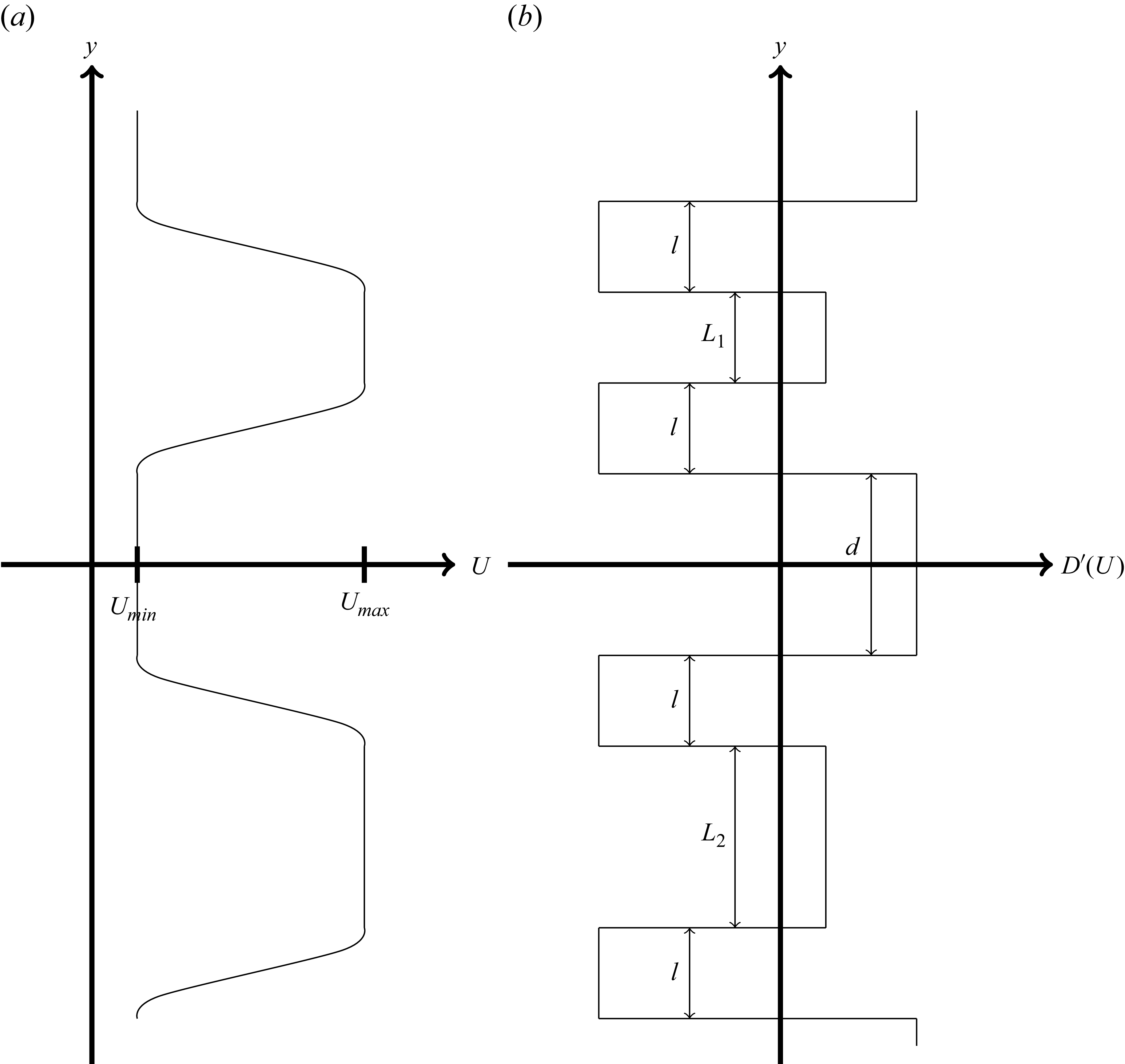
, the streamfunction is a simple linear equation for all space except at the boundaries between regions, which must be handled separately. We construct two jets a distance
 $d$
apart, see figure 13. The jets have velocity of
 $ U_{\textit{max}}$
, and sizes of
 $L_1$
and
 $L_2$
with two adjacent transition regions, each of size
 $l$
. Likewise, the dead zones on the other side of the transition have velocity
 $U_{\textit{min}}$
. The two jets, two dead zones, and four transition regions create eight disparate regions of constant
 $D'$
, each of which has a streamfunction perturbation of
 \begin{equation} \tilde {\psi }_i=e^{\lambda t+i\omega t}\sum _{\!j}\hat {\psi }^j_ie^{\kappa ^j_i y}, \end{equation}
where the superscript
 $j$
indicates the possible roots of the following characteristic equation:
 \begin{equation} (\lambda +i\omega )\kappa _i-\beta \sin (\overline {\theta })=-D'(U_i)\kappa _i+\nu (\kappa _i)^3. \end{equation}
Diagram showing the set-up for the piecewise jet problem. (a) Velocity structure for reference and (b) derivative of the drag function in space.

The solution for
 $\overline \theta =0$
is considerably simpler because it has only two unique roots, so we investigate this case first. First, we need to understand the general structure of quasi-steady solutions. The equation for the evolution of a zonal flow follows:
 \begin{equation} \frac {\partial }{\partial t}\frac {\partial }{\partial y}\varPsi =-{D}(|\boldsymbol{U}|)+\nu \frac {\partial ^3}{\partial y^3}\varPsi + \frac {1}{A}\iint D(|\boldsymbol{U}|)\,\text{d}x\text{d}y, \end{equation}
which becomes a reasonably simple differential equation to solve for a steady state. In practice (see figure 8), the mean value of
 $D$
(over the full dynamical range of
 $U$
seen in these simulations) is very nearly
 $D(\overline {U})$
. This means that a locally homogeneous jet or dead zone will have velocities given by the intersection of
 $D(U)=D(\overline {U})$
, for which there are three solutions that we will call
 $U_{\textit{max}}$
,
 $\overline {U}$
and
 $U_{\textit{min}}$
, respectively. We can also use this expression to solve for the expected structure where the velocity is not locally homogeneous. If we consider a piecewise form of
 $D$
, with values
 $D_{\textit{min}}$
for
 $U\gt \overline {U}$
and
 $D_{\textit{max}}$
for
 $U\lt \overline {U}$
, we can construct an analytic form for the velocity between the jet and dead zones by solving
 \begin{equation} D_{\textit{min}} - D(\overline {U})=\nu \frac {\partial ^2}{\partial y^2}U, \end{equation}
on the jet side of the transition and
 \begin{equation} D_{\textit{max}} - D(\overline {U})=\nu \frac {\partial ^2}{\partial y^2}U, \end{equation}
on the dead-zone side. These are trivial to solve for
 $U(y)$
, giving two parabolas that can be linked at
 $U=\overline {U}$
(i.e. we require they be continuous and differentiable), and that have
 $\partial U/\partial y=0$
where the transition meets the jet and where it meets the dead zone. The distance between the centres of these parabolas can be found to be related to the parameters of the system by
 \begin{equation} l^2=2\nu \frac {(U_{\textit{max}}-U_{\textit{min}})\left (D_{\textit{max}}-D_{\textit{min}}\right )}{\left (D_{\textit{max}}-D(\overline {U})\right )\left (D_{\textit{min}}-D(\overline {U})\right )}, \end{equation}
which comes to a distance of roughly 44 km for the parameters in this study, well in agreement with the size of the transition regions in the bottom layer of figure 7, for example.
With the general structure and values understood, we can examine the stability conditions for jets and waves in this configuration. We can gain some insight by noting the case of marginal stability. In this case, (B8) becomes
 $(\kappa _i)^2=D'(U_i) / \nu$
, so in regions where
 $D'\gt 0$
, the streamfunction perturbations will exponentially weaken with distance from the NMDI-unstable region. We can numerically relate the streamfunction amplitudes by requiring that – at the boundaries of each region – the streamfunction be continuous and differentiable. This creates a matrix equation operating on the
 $\hat {\psi }^j_i$
coefficients where we use (B8) to evaluate the values of
 $\kappa$
. This expression is nonlinear in
 $\lambda$
, so a simple eigenvalue analysis is not possible, but we can find non-trivial solutions by setting the determinant of the matrix to be zero and numerically solving for the largest possible value of
 $\lambda$
. This represents the growth rate of any instabilities possible from the interactions between these two jets. We find that the system is unstable if
 $L_1,L_2\lesssim 8.4\sqrt {\nu /D'(U_{\textit{max}})}$
or
 $d\lesssim 6.7\sqrt {\nu /D'(U_{\textit{min}})}$
, or in dimensional units for these parameters, if
 $L_1,L_2\lesssim 80$
km or
 $d\lesssim 40$
km. In the case where we wish to measure the extents from the centre of the transition regions instead, adding
 $l$
to these gives the total distances.
For non-zonal flows, the behaviour changes dramatically, as growing wave solutions are possible and we can examine their behaviour. Taking (B8) for
 $\kappa _{\!j}\rightarrow ik$
, where
 $k\in \mathcal{R}$
, we find that the slope of wave solutions grows at a rate
 \begin{equation} \lambda =-D'(U_i)-\nu k^2, \end{equation}
and the wave dispersion relation is
 \begin{equation} \omega =-\frac {\beta }{k}\sin (\overline {\theta }). \end{equation}
In this case, stationary jet solutions are no longer possible and most structures will disperse over time. Typically, we expect the fastest growing mode to develop until the maximum and minimum velocities are near
 $U_{\textit{max}}$
and
 $U_{\textit{min}}$
, respectively, and we can consider the behaviour of another linearly unstable wave superimposed on this one with larger wavenumber. Because the waves travel at different speeds, the new wave will eventually cause changes in the maximum and minimum values of velocity from
 $U_{\textit{max}}$
and
 $U_{\textit{min}}$
, which the nonlinear drag will suppress, damping the wave with higher wavenumber. Though the original wave will also be damped slightly, the effect is more prominent for the larger wavenumber (because the oscillations will average out over longer spatial scales). This generally causes the wavelength of the produced Rossby waves to differ substantially from the NMDI linear theory, producing much larger wavelengths in nonlinear simulations than would ordinarily be expected.

 Nx=Ny=768
 Nx=Ny=1152

 h=300

 h=300

 h=300


 h=300
 θ¯=0
 kmin=2π/10
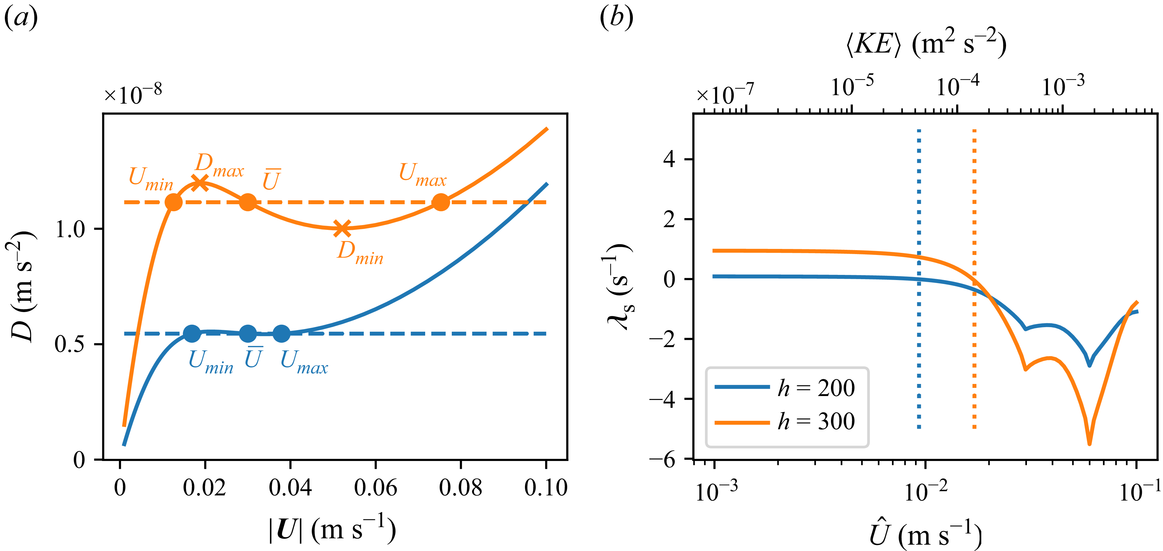
 h=200
 h=300
 D
 Umin
 Umax
 Dmin
 Dmax

 h=300

 h=300