2.1. Model with No Deterministic Terms

Consider first the p-dimensional VAR model of order k with no deterministic terms as given by

Here Π, Γ, and Ψ_i are p × p matrices, ε_t is a p-dimensional independent and identically distributed (i.i.d.) N_p(0,Ω) sequence, Ω > 0, and the initial values X_−k+1,…, X₀ are fixed for the statistical analysis. The I(2) model, denoted H(r,s), is then defined by two reduced rank restrictions given by

where α and β are p × r matrices and ξ and η are (p − r) × s matrices with r ≤ p and s ≤ p − r. We use the notation H(r) = H(r,p − r) to denote I(1) models, and H(p) denotes the unrestricted vector autoregression.

2.1.1. Representation.

To state a representation for X_t, denote by H₀(r,s) the assumption that the characteristic polynomial, A(z) = I_p(1 − z)² − Πz + Γ(1 − z)z − Ψ₁(1 − z)²z − ··· − Ψ_k−2(1 − z)²z^k−2, has exactly 2(p − r) − s roots at z = 1 and the remaining roots outside the unit circle. It relates to H(r,s) as the 2(p − r) − s unit roots imply reduced rank r < p in (2) and reduced rank s < p − r in (3).

Under H₀(r,s), X_t in (1) is an I(2) process with the representation

By Johansen (1992), X_st is a stationary mean-zero I(0) process, and the notation α₁ = α_⊥ξ, β₁ = β_⊥η, α₂ = (α,α₁)_⊥, β₂ = (β,β₁)_⊥, and

has been used. The coefficients γ_c and γ_l depend on the initial values of the process and satisfy (β,β₁)′γ_l = 0 and β′γ_c − δβ₂′γ_l = 0, where δ = α′Γβ₂. It follows from (4) that (β,β₁)′X_t is I(1) as (β,β₁)′C₂ = 0, whereas the (p − r − s) linear combinations β₂′ X_t are I(2). Moreover, there are r mean-zero stationary linear combinations,

2.1.2. Variation-Free Parametrization.

To maximize the likelihood function for known ranks (r,s) under the hypothesis H(r,s), Johansen (1997) suggested a reparametrization of the model based on the reduced ranks in (2) and (3) and also on the cointegration term in (5). The reparametrization is given by

where

. Furthermore, α, ρ ((r + s) × r), τ (p × (r + s)), ψ (p × r), κ ((r + s) × (p − r)), Ψ_i (p × p), i = 1,…, k − 2, and Ω are all freely varying parameters. The parameters in the previous formulation in (1)–(3) can be derived from the new parameters by the identities τ = (β,β₁), β = τρ,

,

, and κ′ = −α_⊥′Γ(β,β₁) = −(α_⊥′Γβ,ξ), using the skew-projection identity,

No closed form solution for the ML estimators of the parameters in (6) exists, but estimates are obtained by a switching algorithm: for fixed τ, the parameters α_⊥ and α can be obtained by solving an eigenvalue problem, and the remaining parameters can be found from regression. For fixed values of these parameters, τ can be estimated by generalized least squares. Convergence to the global maximum of the likelihood function is not guaranteed, but the value of the likelihood function increases in each iteration. In our implementations we use the two-step estimators, reviewed next, as starting values for the ML iterations.

In the two-step estimation, first the parameters α and β in (2) are estimated by RRR as applied in I(1) models ignoring the reduced rank restriction (3). In the second step, ξ and η in (3) are estimated by RRR with r and the estimated α and β from the first step fixed; see Johansen (1995).

2.2. Models with Linear Trends and Deterministics

It is often important to include deterministic linear trends and a constant level in empirical applications. Rahbek et al. (1999) propose an I(2) VAR model that allows deterministic linear trends and a constant level in all components and linear combinations of the process. This includes the cointegrating relations (5) and avoids at the same time the possibility of quadratic trends. In terms of the parameterization in (6), this model, denoted H*(r,s), can be represented as

where τ* = (τ′,τ_l)′ ((p + 1) × (r + s)), ψ* = (ψ′,ψ_c)′ ((p + 1) × r), and, finally, X_t* = (X_t′,t)′ is p + 1-dimensional. As in Section 2.1.1, the model with exactly 2(p − r) − s unit roots and the remaining roots with modulus larger than one is referred to as H₀*(r,s). Under H₀*(r,s) the process X_t in (8) has the representation in (4) but with γ_l and γ_c being functions of τ_l and ψ_c in addition to initial values. In particular, Δ²X_t,

are mean-zero stationary processes. As a result, X_t is as emphasized an I(2) process with linear trends in all linear combinations of the process. With X_t* and ΔX_t* replacing X_t and ΔX_t, respectively, ML estimation of the parameters under H*(r,s) is identical to the case of no deterministic terms. Asymptotic distributions of the ML estimators can be found in Rahbek and Nielsen (2006), and two-step-based inference is discussed in Rahbek et al. (1999).

Further classes of I(2) models with varying deterministic specifications have been considered in the literature, such as, e.g., the model with a constant level in all linear combinations of the process, including the cointegrating. In this case the model can be represented as in (8), with X_t* = (X_t′,1)′ and ΔX_t* = ΔX_t. Models with this and also with different specifications of the parameter of the constant regressor are considered in Paruolo (1996, 2000).

3.1. Test Statistics

For rank determination we propose to use the LR test for H(r,s) against the unrestricted alternative, H(p), as defined by

where

and

denote the covariance matrices estimated under H(r,s) and H(p), respectively. The conventionally applied two-step rank test statistic is the sum of two test statistics:

where

and

. Here λ_i are the (p − r) smallest eigenvalues from the RRR in the first step, and ζ_i are the (p − r − s) smallest eigenvalues from the RRR in the second step of the two-step estimation, corresponding to the reduced ranks of Π and α_⊥′Γβ_⊥ in (2) and (3), respectively. Likewise for H*(r,s) and H*(p), in which case the LR test is denoted S_r,s^LR* and the two-step test is denoted S_r,s^2S*.

3.2. Asymptotic Distributions of the LR Tests

In this section the asymptotic distributions are given for the LR tests of cointegration ranks in the I(2) models H(r,s) and H*(r,s). To present the limiting distributions define for X_u, Y_u, and Z_u of dimension p_x, p_y, and p_z on the unit interval u ∈ [0,1],

Consider first the hypothesis H(r,s) against the unrestricted H(p).

THEOREM 1. Under H₀(r,s) (cf. Section 2.1.1), then as T → ∞,

where

Here W_u = (W_1u′,W_2u′)′ is a (p − r)-dimensional standard Brownian motion on the unit interval, u ∈ [0,1], with W_1u of dimension s and W_2u of dimension p − r − s. Furthermore,

The proof is given in Appendix A. Note, that the asymptotic distribution of the LR test is identical to the asymptotic distribution of the two-step rank test derived in Johansen (1995, Thm. 7). In particular, the two components, Q_r^∞ and Q_r,s^∞, have the asymptotic distributions of the statistics from the first and second steps of the two-step rank test, Q_r and Q_r,s. This implies that the critical values for the two-step rank test can be applied to the LR test.

The result in Theorem 1 is extended to the model H*(r,s) in Theorem 2. The proof given in Appendix B is based on asymptotic theory in Rahbek and Nielsen (2006) for the ML estimators of the parameters in H*(r,s). An important implication is that the LR test and the two-step test are asymptotically similar with respect to the parameters of the deterministic terms; see also Nielsen and Rahbek (2000) for a discussion of the implication of similarity. Critical values are given in, inter alia, Rahbek et al. (1999) and Doornik (1998).

THEOREM 2. Under H₀*(r,s), then as T → ∞,

where Q_r*^∞ = tr{S(W,G₁,W)} and Q_r,s*^∞ = tr{S(W₂,G₂,W₂)}. The Brownian motion W_u is defined in Theorem 1, and

The results in Theorems 1 and 2 can be extended to further classes of I(2) models. Specifically, Paruolo (2000) showed that the two-step estimators are asymptotically efficient for a wide class of models including the case of a constant level in all linear combinations of the process. Hence mimicking the proofs of Theorems 1 and 2 and using Paruolo (1996), the limiting distribution of the LR test for cointegration ranks is conjectured to be the same as reported in Theorem 2, but with

and G₂ = W_2u.

3.3. Rank Determination

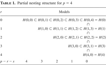
Different values of the cointegration ranks define the sequence of partially nested models illustrated in Table 1 for the p = 4-dimensional case, and we discuss rank selection for the model with no deterministic terms for simplicity.

Partial nesting structure for p = 4

In the determination of the cointegration ranks in empirical applications, economic theory may provide some guidance. With a particular model suggested by theory, the corresponding hypothesis, H(r,s), can be tested directly against H(p). Alternatively, or if little is known a priori, an estimate

of the ranks can be obtained by a sequential application of the rank tests. The idea is to start testing the most restricted model, H(0,0), and in case of rejection to proceed left to right and top to bottom in Table 1. The estimator can be written as

where S_r,s denote either of the test statistics and c_r,s their asymptotic critical values. The estimator

will select the correct ranks with a limiting probability (1 − π), where π is the size of each test in the sequence as discussed in Johansen (1995).

4.1. The LR and Two-Step Statistics in Finite Samples

The asymptotic equivalence of the LR test and the two-step rank test does not hold for finite samples in general. The relation between the test statistics is stated in the following proposition for the case of H(r,s). Note that the same result holds for H*(r,s).

PROPOSITION 1. Consider the hypothesis H(r,s) in H(p). In finite samples,

Equality holds if (p − r − s)r = 0.

Proof. First note that the LR test, S_r,s^LR, is given in (9) as

, where

and

denote the covariance matrices found by ML estimation under H(r,s) and H(p), respectively. The two-step-based test, S_r,s^2S, in (10) can be rewritten as

where

is the two-step-based estimator of Ω under H(r,s) and

is the (ML) estimator of Ω under H(r) = H(r,p − r). Thus, S_r,s^LR ≤ S_r,s^2S is equivalent to

. This follows by showing that (i) the two-step-based estimators of the parameters are not ML estimators and, at the same time, (ii) the parameters of the two-step parametrization lie in the parameter set over which the ML estimation is performed. To see this, note that the estimator

is found by maximizing the likelihood function as defined by (6), with freely varying parameters in the parametrization as given by θ_LR := (α,ρ,τ,ψ,κ,Ψ_i,Ω). The estimator

is best discussed in the variation-dependent parametrization given by θ_2S := (α,β,ξ,η,α_⊥′Γβ,α′Γ,Ψ_i,Ω). Fixing β and α at their first step RRR values,

is found by maximizing the likelihood function over the remaining parameters in θ_2S. Setting α = α, τ = (β,β_⊥η), ρ = (I,0)′, Ω = Ω,

, κ′ = −(α_⊥′Γβ,ξ), and Ψ_i = Ψ_i, this corresponds to a specific parameter point in θ_LR, and, by definition,

. Note that in two special cases, the two-step procedure actually maximizes the likelihood function under H(r,s): first, in I(1) models, where s = p − r and α_⊥′Γβ_⊥ is nonsingular; and second, if r = 0 where the second step of the two-step procedure is conditional on α = β = 0. █

Proposition 1 implies that rejection frequencies for hypothesis H(r,s) in H(p), where r(p − r − s) > 0, are lower for the LR test than for the two-step test. As a consequence the type I error probability is lower for the LR test, whereas the type II error probabilities, for tests of more restricted models, are potentially larger.

Note that the magnitude of the difference depends on the number of restrictions in (3), which is ignored in the first step of the two-step estimator. The number of ignored restrictions is largest for models on the diagonal of Table 1, where s = 0, and the LR and the two-step statistics coincide for models located in the first row and last column of Table 1. Also note that in the model H*(r,s) a restriction on the parameter of the constant regressor is ignored in the first step of the two-step procedure. Finally, note that in Proposition 1 the special case of r(p − r − s) = 0 is implied by either no I(2) trends (p − r − s = 0) or by no I(0) relations (r = 0). Under the assumption of I(2), the case of r = 0 implies that Γ has reduced rank s < p and can be factorized as Γ = ξη′, and hence this case mimics the statistical analysis of an I(1) VAR model in first differences.

4.2. Empirical Study and Monte Carlo Simulations

To analyze the small-sample properties and compare the LR and two-step tests, three approaches were taken. First, we revisited the rank determination in a number of published I(2) applications in the literature using both types of statistics. We reconsidered the money demand analyzed by I(2) VAR models in, inter alia, Johansen (1992) and Rahbek et al. (1999), the domestic pricing behavior in Banerjee et al. (2001), the Danish export pricing behavior in Nielsen (2002), and the Danish import price determination in Kongsted (2003). Next, Monte Carlo simulations were performed with the estimated models as data generating processes (DGPs); i.e., for each empirical example a DGP was defined as the model H*(r,s) with parameter values set to the ML estimates. With this choice of DGPs for the Monte Carlo study they were empirically relevant, and we checked that the parameters satisfied the assumptions underlying the theoretical results. Finally, we constructed a larger study based on different DGPs to cover a broader range of the parameter space of the I(2) model.

The main result emerging from the studies is that the size properties of the LR test are clearly preferable to the two-step test and the rejection frequency of the LR test for a true null hypothesis is often close to the nominal size of the test. The two-step test, on the other hand, is often severely size distorted, with rejection frequencies far above the nominal size. This is particularly the case if s = 0 in the DGP. In some cases the LR test still overrejects true hypotheses, as is also known from the LR test in I(1) models. If the size distortion of the LR test is deemed important, the challenging task of deriving a Bartlett correction of the LR test can be considered; see, e.g., Johansen (2002) for the I(1) case. To keep the presentation concise and focus on the main points we report results only for the Danish import price determination. The full set of results can be obtained from the authors.¹

4.2.1. Empirical Illustration.

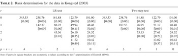
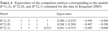
In this section we revisit the rank determination in Kongsted (2003) based on a p = 4-dimensional set of data including Danish import prices, domestic prices, a measure of competing prices, and an interest rate. Kongsted (2003) estimated a VAR(2) model for the effective sample 1975:3–1995:4 and included a linear trend in all directions, corresponding to the model H*(r,s), in addition to an unrestricted impulse dummy for the observation 1992:2. Here we adopt the same specification, noting that the impulse dummy has no effect asymptotically. According to Kongsted (2003), economic theory suggests the model H*(2,1) with two stationary relations, one I(1) trend and one I(2) trend. The LR statistics for the cointegration ranks are reported on the left-hand side of Table 2. Starting from the most restricted model H*(0,0) it is possible to reject all models with r = 0 at a 5% level. In the second row, H*(1,0) and H*(1,1) are easily rejected, whereas H*(1,2) has a p-value of 11%. If this model is nevertheless rejected, the next potential model is H*(2,0), comprising two stationary relations and two I(2) trends, again with a p-value of around 10%. The test statistic for the theoretically preferred model, H*(2,1), is 26 corresponding to a p-value of 35%. The LR rank tests thus point toward the models H*(1,2), H*(2,0), and H*(2,1) as potentially relevant for the current data. The eigenvalues of the companion matrices corresponding to these models, i.e., the inverse roots of the characteristic polynomials, are given in Table 3. The processes have 2(p − r) − s unit roots, and for all three choices of parameter values the remaining roots seem to be far from the unit circle in accordance with the assumptions for Theorem 2.

Rank determination for the data in Kongsted (2003)

Eigenvalues of the companion matrices corresponding to the models H*(1,2), H*(2,0), and H*(2,1) estimated for the data in Kongsted (2003)

The two-step rank test statistics, also reported in Kongsted (2003), are given on the right-hand side of Table 2. As noted, all test statistics in the first row and last column are identical to the LR results, and the remaining test statistics are all higher. Using the two-step test there is marginally more evidence for rejecting H*(1,2). Furthermore, the model H*(2,0) is clearly rejected, and the two-step statistic of 75 is markedly higher than the corresponding LR statistic of 45. Thus based on asymptotic inference with a 5% significance level, both statistics lead to different results than expected from economic theory, and the two tests give different indications on the potentially relevant models. In the next section we use Monte Carlo simulations to investigate further the differences of the two tests in particular with respect to size properties.

4.2.2. Simulations Based on the Estimated Model.

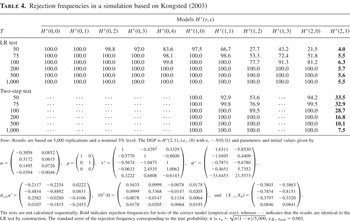
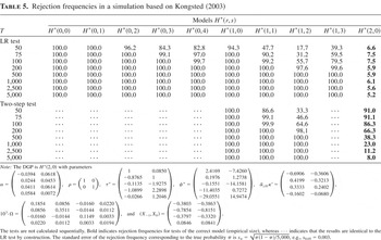
To analyze the differences, we set up a small Monte Carlo simulation with the DGPs defined by the parameters from ML estimation under H*(2,1); see Table 4 for specific parameter values. For each simulation i, we generate time series, X₁ⁱ,… X_Tⁱ, for T ranging between 50 and 1,000 and by replacing ε_t with random draws from an i.i.d. Gaussian distribution with the estimated covariance matrix. Each series is initiated with initial values X₀ⁱ and ΔX₀ⁱ; to ensure that each nonstationary series is initiated the same way across all simulations, the nonstationary I(1) and I(2) directions of the process are initiated from the corresponding observed initial values. That is, with β₂ = τ_⊥, β₂′ X₀ⁱ = β₂′ X₀^obs, β₂′ΔX₀ⁱ = β₂′ΔX₀^obs, and, correspondingly, β₁′ X₀ⁱ = β₁′ X₀^obs. The stationary directions, ρ′τ*′X_tⁱ* + ψ*′ΔX_tⁱ*, τ*′ΔX_tⁱ*, and β₂′Δ²X_tⁱ, are on the other hand initiated from the invariant distribution by discarding 100 initial simulations of the stationary series, thus eliminating the importance of initial values in the stationary series.

Rejection frequencies in a simulation based on Kongsted (2003)

The rejection frequencies at a nominal 5% level are reported in Table 4 for the two tests. The rejection frequencies of H*(r,s) in H*(p) are identical for the two-step rank test and the LR test for models with r = 0. For the models H*(1,0), H*(1,1), H*(1,2), H*(2,0), and H*(2,1), the finite-sample distributions, and the rejection frequencies, differ. For the LR test the rejection frequencies for the true model H*(2,1) are very close to the nominal 5% for all sample lengths. The rejection frequencies of some of the more restricted hypotheses, e.g., H*(1,2) and H*(2,0), are relatively low in small samples, indicating a low power. The two-step test is clearly size distorted, with rejection frequencies for the true model H*(2,1) around 30% in small samples. The actual size converges very slowly to the nominal 5%, and for T = 500 the rejection frequency is still twice the nominal size. At the same time the rejection frequencies for more restricted models are higher than the LR test. For a small sample, T = 50, the rejection frequency for H*(2,0) is 94% compared to a rejection frequency of 22% for the LR test.

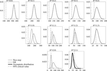
The distributions of the test statistics are reported in Figure 1 for the case T = 75. The graphs are organized according to the nesting structure in Table 1. The lower right graph reports the results for tests of the true model, H*(2,1). The distribution of the LR statistics almost coincides with the asymptotic distribution, whereas the distribution of the two-step statistics is more dispersed and displaced to the right. For some of the more restricted hypotheses, there are big differences between the distributions. The difference is largest if s = 0.

Distributions of the two test statistics for the case T = 75. Graphs are organized according to the partial nesting structure. Results are based on 5,000 replications.

To illustrate the difference when s = 0 in the true model, we performed the simulations again taking ML estimation under H*(2,0) as defining the DGP; see Table 5 for the parameter values. In this case a large distortion appears in the two-step estimation of the model with correct ranks. The rejection frequencies are reported in Table 5. Note that the true model H*(2,0) is almost always rejected using the two-step rank test—and this is the case for all relevant sample lengths. For T = 200, corresponding to 50 years of quarterly observations, the actual size of the two-step test is 66%. The LR tests, on the other hand, have good size properties, with rejection frequencies close to the nominal size.

Rejection frequencies in a simulation based on Kongsted (2003)