1 Introduction
The performance of lifting surfaces operating at relatively low chord-based Reynolds numbers (
 $Re_{c}<10^{6}$
) is often significantly affected by laminar boundary layer separation occurring on the suction side due to the adverse pressure gradient (Carmichael Reference Carmichael1981; Lissaman Reference Lissaman1983; Mueller & DeLaurier Reference Mueller and DeLaurier2003). The laminar boundary layer separation leads to the formation of a separated shear layer, which is inherently unstable to small-amplitude disturbances and, at sufficiently high Reynolds numbers (
 $Re_{c}>10^{4}$
), undergoes transition shortly downstream of separation. At incidence angles below the stall condition, the laminar-to-turbulent transition and the associated enhancement in the exchange of momentum with the outer flow lead to shear layer reattachment in the time-averaged sense. The produced closed flow region above the aerofoil surface is commonly referred to as the laminar separation bubble (LSB), and is the main focus of the present investigation. Note that the term ‘laminar’ in this context refers to the state of boundary layer at separation as opposed to the flow regime in the entire bubble. Due to the influence of the LSB on aerofoil performance, flows involving LSBs have attracted significant research interest over the past several decades. Tani (Reference Tani1964), Gaster (Reference Gaster1967) and Carmichael (Reference Carmichael1981) review the earlier studies on this topic and provide a comprehensive description of the mean bubble topology. Subsequent research efforts have been directed primarily towards laminar-to-turbulent transition in the separated shear layer, which has been recognised as the key phenomenon governing the formation and characteristics of LSBs (Dovgal, Kozlov & Michalke Reference Dovgal, Kozlov and Michalke1994; Lin & Pauley Reference Lin and Pauley1996; Watmuff Reference Watmuff1999; Rist & Maucher Reference Rist and Maucher2002; Jones, Sandberg & Sandham Reference Jones, Sandberg and Sandham2008). An overview of these more recent studies can be found, for example, in Marxen & Henningson (Reference Marxen and Henningson2011) and Boutilier & Yarusevych (Reference Boutilier and Yarusevych2012).
Previous investigations have shown that the transition process in the separated shear layer begins with the amplification of small amplitude disturbances. The initial amplification occurs within a band of unstable frequencies and is well modelled by linear stability theory (Häggmark, Hildings & Henningson Reference Häggmark, Hildings and Henningson2001; Boiko et al. Reference Boiko, Grek, Dovgal and Kozlov2002; Marxen, Lang & Rist Reference Marxen, Lang and Rist2012). The growth of the disturbances is largely governed by a convective, inviscid Kelvin–Helmholtz instability (Boutilier & Yarusevych Reference Boutilier and Yarusevych2012). The viscous effects have been shown to diminish with increasing Reynolds number and distance between the separated shear layer and the wall (Dovgal et al. Reference Dovgal, Kozlov and Michalke1994; Rist, Maucher & Wagner Reference Rist, Maucher and Wagner1996; Diwan & Ramesh Reference Diwan and Ramesh2009). Combining these factors into a Reynolds number based on displacement thickness, Boutilier & Yarusevych (Reference Boutilier and Yarusevych2012) show that viscous damping of the maximum growth rate of disturbances increases with decreasing displacement-based Reynolds number, but does not exceed approximately 15 % of the inviscid growth rate (see their figure 14). As discussed in detail by Diwan & Ramesh (Reference Diwan and Ramesh2009), the slow convective amplification of disturbances through the Tollmien–Schlichting instability in the boundary layer upstream of separation can be viewed as a natural precursor to the significant amplification that occurs in the separation bubble, mainly due to the inflectional instability associated with the Kelvin–Helmholtz mechanism. The small amplitude disturbances convecting into LSB may also influence the later stages of transition (Brinkerhoff & Yaras Reference Brinkerhoff and Yaras2011). An absolute instability can be present in LSBs if reverse flow velocities in the near-wall region bounding the separated shear layer exceed 15 %–20 % of the edge velocity (Alam & Sandham Reference Alam and Sandham2000). A possibility of global instability modes in LSBs has also been suggested (Theofilis, Hein & Dallmann Reference Theofilis, Hein and Dallmann2000; Rodríguez, Gennaro & Juniper Reference Rodríguez, Gennaro and Juniper2013).
As the amplitude of unstable disturbances in the separated shear layer increases, nonlinear interactions become important. The amplification of the instability waves eventually leads to shear layer roll-up and periodic shedding of vortices in the aft portion of the bubble (Watmuff Reference Watmuff1999; Burgmann & Schröder Reference Burgmann and Schröder2008; Yarusevych, Sullivan & Kawall Reference Yarusevych, Sullivan and Kawall2009; Marxen, Lang & Rist Reference Marxen, Lang and Rist2013). These structures dominate the flow development in the aft portion of the bubble (Jones et al. Reference Jones, Sandberg and Sandham2008; Lengani et al. Reference Lengani, Simoni, Ubaldi and Zunino2014; Serna & Lázaro Reference Serna and Lázaro2015), and may be primarily responsible for inducing time-averaged flow reattachment. The vortices form in the aft portion and are subject to significant spanwise deformations prior to a rapid breakdown to smaller scale structures in the vicinity of reattachment (Burgmann & Schröder Reference Burgmann and Schröder2008; Jones et al. Reference Jones, Sandberg and Sandham2008; Hain, Kähler & Radespiel Reference Hain, Kähler and Radespiel2009; Yarusevych et al. Reference Yarusevych, Sullivan and Kawall2009). Brinkerhoff & Yaras (Reference Brinkerhoff and Yaras2011) link the break-up process to the influence of smaller scale streamwise structures that originate due to a viscous instability upstream of separation. In contrast, Jones et al. (Reference Jones, Sandberg and Sandham2008) and Marxen et al. (Reference Marxen, Lang and Rist2013) ascribe the break-up to the elliptic instability of the spanwise vortex filaments and/or the instability originating in the braids (finger vortices) connecting consecutive rollers. The later stages of transition in LSBs remain the subject of active research, including the development and breakdown of shear layer roll-up vortices (Robinet Reference Robinet2013).
The inherent sensitivity of the separated shear layer makes these flows sensitive to small-amplitude free-stream disturbances. While this presents challenges due to possible discrepancies in the results obtained in different simulations and experiments (Ol et al. Reference Ol, Mcauliffe, Hanff, Scholz and Kähler2005; Marxen & Henningson Reference Marxen and Henningson2011; Olson et al. Reference Olson, Katz, Naguib, Koochesfahani, Rizzetta and Visbal2013), it makes possible the application of active flow control methods aimed at modifying LSBs and improving the performance of lifting surfaces. Various flow actuation techniques considered to date have been reviewed by Cattafesta & Sheplak (Reference Cattafesta and Sheplak2011). Periodic excitation using external acoustic waves (Zaman Reference Zaman1992), embedded synthetic jets (Glezer & Amitay Reference Glezer and Amitay2002; Goodfellow, Yarusevych & Sullivan Reference Goodfellow, Yarusevych and Sullivan2012), plasma-based actuators (Corke et al. Reference Corke, Bowles, He and Matlis2011; Rizzetta & Visbal Reference Rizzetta and Visbal2011) and other techniques (Cattafesta & Sheplak Reference Cattafesta and Sheplak2011) have been considered and shown to be capable of inducing flow reattachment on a stalled aerofoil (i.e. inducing the formation of an LSB) and/or reducing the size of an LSB. For optimal performance, the actuator should be placed upstream of laminar separation, and its effect on flow development has been shown to depend on the amplitude and frequency of excitation. Using controlled acoustic excitation, Yarusevych, Sullivan & Kawall (Reference Yarusevych, Sullivan and Kawall2007) have linked the most effective excitation frequency to that of the most amplified disturbances in undisturbed flow. However, in most flow control studies involving LSBs on aerofoils, the main focus was on the changes in mean LSB characteristics and aerofoil performance rather than the attendant changes in bubble dynamics. On the other hand, many detailed studies on LSBs used artificial, small-amplitude disturbances to investigate shear layer transition via numerical simulations (Jones et al. Reference Jones, Sandberg and Sandham2008; Marxen & Henningson Reference Marxen and Henningson2011) and experiments (Watmuff Reference Watmuff1999; Lang, Rist & Wagner Reference Lang, Rist and Wagner2004; Diwan & Ramesh Reference Diwan and Ramesh2009). Marxen & Henningson (Reference Marxen and Henningson2011) show that controlled flow perturbations change the mean topology of the bubble, which the authors refer to as the mean flow deformation, thereby influencing stability characteristics of the LSB. Their results demonstrate that the bubble becomes more stable as the amplitude of the forcing increases. A similar mean flow deformation effect is discussed by Boiko et al. (Reference Boiko, Grek, Dovgal and Kozlov2002). However, they argue that the associated influence on flow stability characteristics is not substantial when the amplitude of artificial disturbances remains relatively small and does not modify the inflectional part of the velocity profiles. Recently, Marxen et al. (Reference Marxen, Kotapati, Mittal and Zaki2015) performed a stability analysis on numerical simulation results of Kotapati et al. (Reference Kotapati, Mittal, Marxen, Ham, You and Cattafesta2010) involving synthetic jet actuation of an LSB. They suggest that the most effective control mechanism relies on convective Kelvin–Helmholtz instability; however, the optimal frequency selection may be affected due to the mean flow deformation induced by the artificial disturbances. These results are yet to be confirmed by an experimental investigation.
One aspect of LSB dynamics that has received little attention in previous studies is the transient response of the bubble to the introduction of artificial disturbances. Particularly, most of the relevant numerical simulations conventionally consider the data pertaining to the quasi-steady state established following the initiation of simulations or the introduction of disturbances. On the other hand, experimental studies of such transients are complicated by the associated requirements on the temporal resolution of the measurement system, as well as technical difficulties associated with the implementation of actuators. However, relevant investigations involving the control of separated flows on various geometries (Darabi & Wygnanski Reference Darabi and Wygnanski2004; Mathis et al. Reference Mathis, Lebedev, Collin, Delville and Bonnet2009; Siauw et al. Reference Siauw, Bonnet, Tensi, Cordier, Noack and Cattafesta2010; Benard et al. Reference Benard, Cattafesta, Moreau, Griffin and Bonnet2011; Asada et al. Reference Asada, Nonomura, Aono, Sato, Okada and Fujii2015) indicate that significant transients produced by the engagement of or changes in flow forcing can occur. Such transients can last on the order of ten convective time scales and are associated with significant changes in structural loads, which makes them important in the design and implementation of flow control techniques. Indeed, it can be inferred from some previous numerical simulations that similar transient flow field changes may occur in LSBs. For example, the results of Jones et al. (Reference Jones, Sandberg and Sandham2008) show significant temporal changes in lift and drag on a NACA 0012 aerofoil when flow forcing is engaged and when forcing is turned off (see their figure 8a). Marxen & Henningson (Reference Marxen and Henningson2011) report that bubble bursting, i.e. rapid enlargement of the LSB, can occur when forcing is turned off. The bursting process continued until the end of their simulations.
The present work investigates the spatio-temporal response of an LSB formed on a NACA 0012 aerofoil to controlled disturbances. While this profile has been used in previous studies on LSB development, e.g. Jones et al. (Reference Jones, Sandberg and Sandham2008), Pröbsting & Yarusevych (Reference Pröbsting and Yarusevych2015), the only critical requirement for the aerofoil geometry in the present investigation is the generation of a representative LSB. The disturbances are introduced just upstream of separation by means of a surface-mounted dielectric barrier discharge (DBD) actuator, and the induced changes in mean topology and dynamics of the separation bubble are investigated by means of time-resolved particle image velocimetry. The goal is to study quasi-steady and transient effects of controlled disturbances on separated shear layer transition and the overall separation bubble dynamics relative to the unperturbed baseline flow. First, the effects of amplitude and frequency of disturbances on the quasi-steady structure of the LSB are investigated, and linear stability analysis is performed to provide added insight into the attendant changes in the flow topology. Then, transient flow development associated with the introduction and removal of controlled perturbations is examined.
2 Experimental set-up
The experiments were performed in a vertical low speed open-jet facility (V-tunnel) at Delft University of Technology. The tunnel has an operating velocity range from approximately 5 to
 $45~\text{m}~\text{s}^{-1}$
. It has an open test section where an axisymmetric jet is formed by a nozzle with an exit diameter of 600 mm. The settling chamber has a contraction ratio of
 $100:1$
and houses a series of flow conditioning devices, resulting in free-stream turbulence levels at the nozzle exit below 0.1 % for the conditions studied here. The free-stream velocity in the test section (
 $U_{0}$
) is set using a Pitot-static tube, with an associated uncertainty of less than 2 %. For the experiments reported here, the tunnel was operated at constant speed of
 $U_{0}=10~\text{m}~\text{s}^{-1}$
.
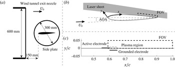
A polycarbonate NACA 0012 aerofoil model, with a chord length of 200 mm and a span of 400 mm (figure 1), was placed approximately 150 mm downstream of the nozzle. Two circular transparent polycarbonate end plates of diameter 300 mm were used in order to mitigate end effects and provide optical access. The spacing between the end plates (400 mm) was selected based on the recommendations provided by Boutilier & Yarusevych (Reference Boutilier and Yarusevych2012) for the use of end plates in experiments involving low Reynolds number flows over aerofoils. The model was mounted along the diameter of the end plates equidistant from the edges of the end plates. The experiments were performed at a geometric angle of attack (AOA) of
 $2^{\circ }$
, which was set using a digital inclinometer with a resolution of
 $0.1^{\circ }$
. In open wind tunnel test sections, the effective angle of attack is typically lower than the geometric angle of attack (Brooks, Marcolini & Pope Reference Brooks, Marcolini and Pope1986). For the present investigation, the effective angle of attack is estimated to be
 $1.2^{\circ }$
. To eliminate any possible influence on the LSB by trailing edge tonal noise produced due to flow separation on the pressure side (Pröbsting & Yarusevych Reference Pröbsting and Yarusevych2015), the boundary layer on the pressure side was tripped using a strip of randomly distributed three-dimensional roughness elements (carborundum, with average grain size of 0.36 mm).
(a) Experimental layout with characteristic dimensions. (b) Aerofoil configuration with body-attached coordinate system. (c) Particle image velocimetry domain and plasma actuator layout (all dimensions to scale).

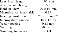
Velocity measurements were performed using a planar, time-resolved, two-component particle image velocimetry (PIV) system. The system comprised of a LaVision Imager Pro HS 4M high speed CMOS camera (
 $2016\times 2016$
pixels sensor, 11
 $\unicode[STIX]{x03BC}$
m pixel pitch) equipped with a Nikon Micro-Nikkor 105 mm lens with aperture number (f
 $\#$
) set to 5.6. A Quantronix Darwin-Duo Nd:YLF laser (30 mJ per pulse at 3 kHz) was used to form an approximately 1.5 mm thick light sheet at the mid-span of the aerofoil model. The camera and laser were synchronised using a LaVision High-Speed controller. The flow was seeded using water–glycol particles with an average diameter of
 $1~\unicode[STIX]{x03BC}$
m introduced in the flow stream upstream of the wind tunnel fan. Particle image pairs were acquired and processed using LaVision Davis 8 software package. The imaged field of view (FOV) was approximately
 $90\times 19$
mm (figure 1), with a magnification factor of approximately 0.25. The camera sensor was cropped to
 $2016\times 428$
pixels and image pairs were recorded at 2 kHz, which is approximately 6.5 times higher than the frequency of the dominant coherent structures in the separation bubble (
 ${\approx}280$
Hz). The acquired image sequences were analysed using a multi-grid, multi-pass correlation algorithm in Davis 8. The final interrogation window size was
 $16\times 16$
pixels, with 75 % overlap resulting in a vector density of 5.6 vectors per mm. For convenience, the main parameters of the PIV measurements are summarised in table 1. The random error in individual velocity fields has been estimated using the particle disparity method proposed in Sciacchitano et al. (Reference Sciacchitano, Neal, Smith, Warner, Vlachos, Wieneke and Scarano2015). The uncertainty in instantaneous velocity measurements outside of the shear layer (i.e. in the outer flow) is less than 1 %, whereas the corresponding uncertainty in shear layer velocity measurements is estimated to be less than 10 % within 95 % confidence limits. As expected, the higher uncertainty is confined to the region of turbulent break-up of coherent structures at and beyond mean reattachment. It should be noted that the quoted values pertain to instantaneous velocity fields, with the relevant uncertainty in mean velocity fields estimated to be less than 4 %. All the velocity measurements are presented in the
 $x$
–
 $y$
surface-attached coordinate system (figure 1). The
 $x$
-axis originates at the leading edge of the aerofoil and is aligned with the aerofoil surface, while the
 $y$
-axis is locally normal to the aerofoil surface and the corresponding coordinate is measured from the surface.
Main PIV system parameters.

Controlled flow disturbances were introduced into the attached laminar boundary layer by means of a dielectric barrier discharge plasma actuator (Corke, Enloe & Wilkinson Reference Corke, Enloe and Wilkinson2010; Benard & Moreau Reference Benard and Moreau2014; Kotsonis Reference Kotsonis2015). The inherent high dynamic range and frequency response of the plasma actuator effectively render the device into a deterministic vibrating ribbon (Ashpis & Reshotko Reference Ashpis and Reshotko1990). The actuator consisted of two thin self-adhesive copper electrodes separated by polyimide dielectric (Kapton), 30 and 110
 $\unicode[STIX]{x03BC}$
m in thickness, respectively. Preliminary investigations revealed no significant effect of the actuator mechanical roughness on the development of the LSB. The actuator components were directly attached to the aerofoil surface 120 mm (
 $x/c=0.6$
) downstream of the leading edge, just upstream of the mean separation location on the suction side (figure 1), and were centred on the mid-span plane. The electrodes measured 10 mm in the streamwise direction and 120 mm in the spanwise direction. The actuator was powered using a TREK 20/20C amplifier. The actuation signal was generated digitally using LabVIEW software and supplied to the amplifier through a compact-data acquisition (compact-DAQ) system, clocking at 100 kHz. The same system was used in order to monitor the delivered voltage and current to the actuator.
Induced velocity due to DBD plasma actuation in quiescent conditions (
 $V_{pp}=5$
kV,
 $c_{\unicode[STIX]{x1D707}}=2\times 10^{-6}$
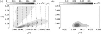
). Time-averaged velocity magnitude field
 $\langle (u^{2}+v^{2})^{0.5}\rangle$
and streamwise velocity fluctuations
 $u_{rms}$
.

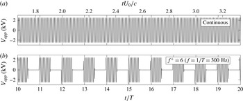
Sample of the applied voltage signal for (a) continuous and (b) pulsed actuation. Peak-to-peak voltage amplitude is 5 kV.

The DBD plasma actuator was characterised in quiescent environment. A representative time-averaged velocity field is depicted in figure 2, pertaining to continuous excitation at frequency of 5 kHz and peak-to-peak applied voltage of 5 kV (figure 3
a). As discussed in detail by Kotsonis & Ghaemi (Reference Kotsonis and Ghaemi2011), the actuator produces a micro-jet, aligned at an angle to the surface and oriented in the general direction of the free stream. The velocity of the jet fluctuates periodically, following the fluctuations in the periodic excitation voltage. In this manner, periodic disturbances at a relevant hydrodynamic frequency can be introduced into the flow by exciting the actuator by either a periodic voltage signal at the relevant carrier frequency or by pulsed actuation, referred to as continuous and pulsed mode, respectively. Due to the relatively low hydrodynamic frequencies of interest in the present study (
 ${\approx}300$
Hz), it was not possible to operate the DBD actuator in a continuous mode (Kotsonis & Ghaemi Reference Kotsonis and Ghaemi2011). Instead, pulsed mode actuation was used to excite hydrodynamic instabilities, similar to a number of previous studies involving synthetic jets (Glezer & Amitay Reference Glezer and Amitay2002) and DBD plasma actuators (Michelis & Kotsonis Reference Michelis and Kotsonis2015). A continuous excitation voltage applied at a carrier frequency of 5 kHz was used (figure 3
a) as the base signal, with the carrier frequency being at least an order of magnitude higher than the highest frequency of interest in the flow investigated. To introduce relevant hydrodynamic disturbances, a square wave modulation of the excitation voltage was used (figure 3
b). A range of modulation frequencies (
 $f$
) from 100 Hz to 500 Hz (
 $2\leqslant f^{+}\leqslant 10$
, where
 $f^{+}=fc/U_{0}$
) was investigated. As will be illustrated later, this range of frequencies was selected based on the range of unstable frequencies in the undisturbed separation bubble.
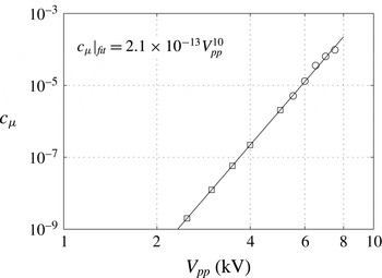
Momentum coefficient of the DBD plasma actuator as function of applied voltage. Measured values (○) and predicted values (▫). The solid line corresponds to the indicated power-law fit.

To study the effect of excitation amplitude, a range of peak-to-peak applied voltage signals from 2 to 5 kV peak-to-peak was considered. For a given voltage amplitude, the duty cycle was adjusted for each modulation frequency to yield the same momentum input per pulse across the investigated range of modulation frequencies. Additionally, it is well known that the amplitude of forcing associated with DBD plasma actuation is nonlinear to the applied voltage (Benard & Moreau Reference Benard and Moreau2014). As such, the amplitude of produced flow excitation was characterised using a conventional definition for momentum coefficient,
 $c_{\unicode[STIX]{x1D707}}=J/q_{\infty }c$
(Kotsonis, Pul & Veldhuis Reference Kotsonis, Pul and Veldhuis2014), where
 $J$
is the total momentum flux of the induced jet per unit length of actuator in quiescent conditions,
 $q_{\infty }$
is the free-stream dynamic pressure and
 $c$
is the aerofoil model chord. In the current work, the actuator’s momentum coefficient has been calculated using direct reaction force measurements from a high accuracy load cell (accuracy of 1 mg) (Kotsonis et al.
Reference Kotsonis, Pul and Veldhuis2014), where the measured reaction force per unit length of the actuator gives
 $J$
. It must be noted here that due to the relatively low applied voltage values used in this study the produced thrust was below the resolution limit of the load cell. In order to rectify this, measurements at higher voltage values were performed and momentum coefficients at lower voltages were estimated based on a fitted power law as shown in figure 4. Based on the mean square error of the fit residuals, the uncertainty in the extrapolated
 $c_{\unicode[STIX]{x1D707}}$
values (i.e. goodness of fit) is estimated to be within
 $\pm 10^{-10}$
. Momentum coefficients presented in figure 4 serve to quantify the forcing amplitude for all excitation cases considered in this study.
To study the quasi-steady effect of controlled disturbances on the flow development, PIV measurements were performed at least 100 convective times after the initiation of disturbances. For capturing transient effects associated with the introduction of disturbances or their removal, PIV measurements were synchronised with the actuator excitation signal. The excitation voltage was sampled simultaneously with camera and laser pulse trigger signals using the compact-DAQ system. This allowed identifying the time at which artificial disturbances were turned on/off in relation to the acquired velocity fields to within 1
 $\unicode[STIX]{x03BC}$
s.
3 Results
All experiments reported here were performed at an angle of attack of
 $2^{\circ }$
and a chord-based Reynolds number (
 $Re_{c}$
) of 130 000. For the conditions investigated, the response of the separation bubble forming on the suction side of the aerofoil to controlled, two-dimensional disturbances introduced by means of the surface-mounted plasma actuator are considered. The results are presented in two sections. The first section presents the quasi-steady response of the separation bubble for a range of excitation frequencies and amplitudes, where measurements were performed once the flow field reached a quasi-steady state following the engagement of the actuator. The second section considers the transient response of the bubble to the introduction and removal of controlled disturbances. It should be noted that all results are presented using surface attached coordinates defined in figure 1.
3.1 Quasi-steady response
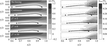
Figure 5 depicts the effect of forcing frequency on the mean and root-mean-square (rms) fields of the streamwise velocity component. The momentum coefficient for all the forced cases is kept constant at
 $c_{\unicode[STIX]{x1D707}}=5.8\times 10^{-8}$
(
 $V_{pp}=3.5$
kV). The results pertaining to the baseline case (no forcing) reveal the presence of a separation bubble within
 $0.6\lesssim x/c\lesssim 0.95$
, marked in figure 5 using a dividing streamline and the estimated locations of mean separation and reattachment. The contours of rms streamwise velocity fluctuations indicate the growth of disturbances in the separated shear layer and in the reverse flow region close to the wall. Distinct triple peaks emerge in the streamwise fluctuating velocity profiles in the aft portion of the bubble, agreeing with the results from previous studies (Boiko et al.
Reference Boiko, Grek, Dovgal and Kozlov2002; Boutilier & Yarusevych Reference Boutilier and Yarusevych2012). The dashed line in figure 5 traces the locations of the maxima in streamwise velocity fluctuations, and corresponds to the location of the second peak from the wall in
 $u_{rms}$
contours, located in the core of the separated shear layer where the highest growth of the disturbances is expected (Dovgal et al.
Reference Dovgal, Kozlov and Michalke1994).
Time-averaged (
 $\langle u\rangle$
) and fluctuating (
 $u_{rms}$
) streamwise velocity fields for different forcing frequencies. Time-averaged dividing streamline (thick solid line), loci of maximum streamwise fluctuations (dashed line), mean separation point (
 $\blacklozenge$
) and mean reattachment point (●).

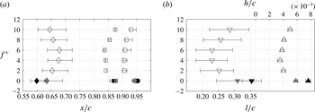
Time-averaged LSB topology as a function of forcing frequency. (a) Locations of separation point (
 $\diamondsuit$
), maximum bubble height (▫) and reattachment point (○). (b) Bubble length (▿) and maximum bubble height (▵). Solid black symbols denote no forcing and solid grey symbols denote continuous forcing.

Introducing continuous forcing at the carrier frequency (
 $f^{+}=100$
) diminishes both the streamwise and vertical extent of the bubble. Since the carrier frequency is well removed from the characteristic flow frequencies, the induced changes are attributed to the mean injection of momentum in the vicinity of the separation location (figure 2), which acts to delay separation. The effect of the forcing becomes more pronounced when the modulated excitation is used to introduce disturbances at lower frequencies within
 $2\leqslant f^{+}\leqslant 10$
, which are of the same order as the characteristic time scales of disturbances expected to develop in the separated shear layer. Forcing at these frequencies increases the amplitude of velocity fluctuations at a given downstream position in the separated shear layer, with the same levels of velocity fluctuations attained earlier upstream in smaller bubbles. Since the forcing amplitude is kept constant, it can be conjectured that disturbances introduced at particular frequencies are more amplified in the separated shear layer, leading to a more significant effect on the mean extent of the bubble. The variation in the location and size of the bubble with forcing frequency is presented in figure 6. The results illustrate that forcing frequency has a significant effect on the streamwise and vertical extent of the bubble, with the minimum bubble size attained at
 $f^{+}\approx 6$
.
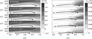
To investigate the effect of forcing amplitude on the time-averaged flow topology, controlled disturbances of varying amplitude were introduced at a fixed frequency of
 $f^{+}=6$
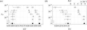
. The effect on the streamwise velocity field is illustrated in figure 7, showing that the size of the separation bubble is progressively diminished by increasing excitation amplitude. Similar to figure 5, the diminishment of the separation bubble correlates with the upstream advancement of shear layer transition. Figure 8 presents the variation of the locations of mean separation, maximum bubble height and reattachment, as well as the streamwise and vertical extent of the bubble, for all the forcing amplitudes investigated. It can be seen that changes in the mean baseline flow are attained only above some amplitude threshold (
 $c_{\unicode[STIX]{x1D707}}\approx 2\times 10^{-9}$
), below which no substantial effect is observed. It is speculated that the minimum amplitude threshold corresponds to the amplitude of natural perturbations attained in the attached boundary layer at the location of the actuator. Once the threshold value is exceeded, the increase in excitation amplitude leads to delayed mean separation and the upstream advancement of the mean reattachment location (figure 8
a), leading to the overall decrease in bubble size (figure 8
b). Yarusevych et al. (Reference Yarusevych, Sullivan and Kawall2007) observed a similar effect of excitation amplitude on the laminar separation bubble in their experiments involving external acoustic forcing. The present results also show that the decrease in streamwise extent of the bubble with increasing forcing amplitude is nearly exponential (figure 8
b). In their direct numerical simulations, Marxen & Henningson (Reference Marxen and Henningson2011) also report a nearly exponential variation in the mean separation and reattachment locations, and, hence, the bubble length, with increasing amplitude of disturbances introduced upstream of separation.
Time-averaged (
 $\langle u\rangle$
) and fluctuating (
 $u_{rms}$
) streamwise velocity fields for different forcing amplitudes. Time-averaged dividing streamline (thick solid line), loci of maximum streamwise fluctuations (dashed line), mean separation point (
 $\blacklozenge$
) and mean reattachment point (●).

Time-averaged LSB topology as function of forcing amplitude. (a) Locations of separation point (
 $\diamondsuit$
), maximum bubble height (▫) and reattachment point (○). (b) Bubble length (▿) and maximum bubble height (▵). Solid black symbols denote no forcing.

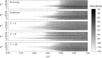
To investigate the development of disturbances in the separated shear layer, spectra of the wall-normal velocity fluctuations are presented in figure 9. The analysed data pertain to the locations of maximum velocity fluctuations (marked by dashed lines in figure 5) attained in the core of the separated shear layer due to the amplification of disturbances. All the forced cases correspond to a constant forcing amplitude of
 $c_{\unicode[STIX]{x1D707}}=5.8\times 10^{-8}$
. For the baseline case (no forcing), the results reveal the amplification of disturbances in a band of frequencies
 $4\lesssim F^{+}\lesssim 8$
, with the most amplified disturbances associated with
 $F^{+}\approx 6$
. The amplified band of frequencies is identifiable in the baseline spectra at and beyond
 $x/c\approx 0.82$
. As the disturbances develop downstream, the amplified frequency band broadens gradually, until a rapid broadening of the energy content over a wide range of frequencies occurs at
 $x/c\approx 0.87$
. This corresponds to the location of the maximum bubble height (figure 6
b), and marks the final stages of laminar to turbulent transition, followed by the mean flow reattachment shortly downstream (figure 5).
Power spectral density of the fluctuating wall-normal velocity component (
 $v^{\prime }$
) probed at the wall-normal location of maximum fluctuations.

For continuous excitation (
 $f^{+}=100$
), a similar trend is observed in the spectra. The unstable frequency band broadens, but the most amplified disturbance frequency remains at
 $F^{+}\approx 6$
. However, when forcing is applied at frequencies close to the unstable frequency range, significant changes in the development of disturbances are observed. Specifically, the primary growth of disturbances occurs within a narrow range of frequencies associated with the excitation frequency and its harmonics. The disturbances attain stronger amplitudes farther upstream as the excitation frequency approaches that of the most amplified disturbances in the baseline case, similar to the trend in the reduction of the extent of the bubble size observed in figure 5. For
 $f^{+}=2$
, the most significant amplification is attained at higher harmonics of the excitation frequency, i.e.
 $F^{+}=4$
, 6 and 8. The most significant effect on the spectral energy content is observed for
 $f^{+}=6$
, where the amplification of the disturbances locks primarily onto
 $F^{+}=6$
, as well as the first two harmonics. Similar effect is observed at
 $f^{+}=10$
; however, a significant amplification is seen at the lower frequency band
 $4\lesssim F^{+}\lesssim 8$
, similar to the amplified frequency band in the baseline case. The results indicate that the artificial disturbances are most amplified when their frequency falls within the band of the most unstable disturbances in the shear layer. In this case, higher amplitude velocity fluctuations are attained earlier due to the amplification of disturbances centred at the excitation frequency, resulting in the most significant diminishment of the separation bubble. In contrast, when the forcing frequency differs substantially from the most unstable frequencies, the development of disturbances is not augmented as effectively through the stability mechanism, and the transition process gradually switches to that driven by a broader frequency band amplification of natural disturbances in the separated shear layer.
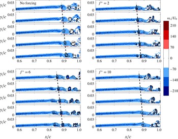
Instantaneous spanwise vorticity fields for different forcing frequencies. Contours based on the
 $\unicode[STIX]{x1D706}_{2}$
criterion are superimposed. Each snapshot is separated by 0.025 convective time scale (
 $tU_{0}/c$
).

Figure 10 depicts the unsteady nature of the separation bubble development using sequences of instantaneous spanwise vorticity fields pertaining to the baseline case and several forcing frequencies applied at a constant amplitude of
 $c_{\unicode[STIX]{x1D707}}=5.8\times 10^{-8}$
. For both the baseline and forced cases, the results show a roll-up of the separated shear layer in the aft portion of the bubble and periodic shedding of vortices. Comparing these results with figures 5 and 6, it can be concluded that the shear layer rolls up just upstream of the streamwise location of the maximum mean bubble height, where the most amplified disturbances reach significant amplitudes. The periodic nature of these structures, in conjunction with spectral results (figure 9) showing distinct spectral peaks in wall-normal velocity fluctuations where vortices form, suggest that the roll-up vortices develop as a consequence of the disturbance amplification in the shear layer. It is evident that the dynamics of the bubble is largely governed by the development of the shear layer vortices. The formation of these structures precipitates the mean flow reattachment by entraining higher momentum fluid from the outer flow into the near-wall region. The classical mean bubble topology, particularly in the aft portion of the bubble, is not reflective of the highly unsteady nature of the flow dominated by the shear layer vortices, and the concept of flow reattachment is applicable mainly in the time-averaged sense.
To aid vortex identification, contours of
 $\unicode[STIX]{x1D706}_{2}$
criterion magnitude (Jeong & Hussain Reference Jeong and Hussain1995) are plotted in figure 10. The dashed lines are drawn through the approximate location of the vortex cores in figure 10, providing estimates of the streamwise wavelength and convective velocity of the structures, related to the streamwise distance and slopes of the lines, respectively. The results indicate that the convective velocity of the structures remains approximately constant (
 ${\approx}0.6U_{0}$
) between the baseline and forced cases. In contrast, the streamwise wavelength scales inversely with the frequency of the most amplified disturbances in each case, as expected for travelling waves of constant propagation speed. The time sequences in figure 10 show that the roll-up location changes with excitation frequency, following the movement of the mean separation bubble in figure 5. The shear layer roll-up becomes more pronounced when the excitation is applied close to the naturally amplified frequencies. For all the cases, the vortices begin to break up downstream of the roll-up location, as can be deduced from the appearance of opposite sign vorticity regions within distinct vortex cores. The onset of this process is reflected in the broadening of the frequency content in the velocity spectra in figure 9, which occurs near the mean reattachment point. However, the break-up is delayed when the excitation is applied at the frequency close to that of the most unstable band in the base flow, as can be seen from a comparison of baseline (no forcing) and
 $f^{+}=6$
data in figure 10. It can be inferred from the results that forcing the flow at these frequencies produces earlier formation of more coherent spanwise vortices in the shear layer, bringing about the reduction in the extent of the separation bubble.
The results discussed up to this point indicate that periodic disturbances introduced at a frequency close to the band of unstable frequencies in the baseline flow produce the most substantial influence on flow development. The most significant effect on separation bubble is observed when forcing is applied close to the frequency of the most amplified disturbances in the baseline flow. To examine this in more detail, a linear stability analysis was performed on the experimental data. The development of shear layer disturbances is modelled via the Orr–Sommerfeld equation (e.g. Schmid & Henningson Reference Schmid and Henningson2001) in the spatial stability formulation, i.e. modelling the convective amplification of disturbances. In the analysis, measured mean streamwise velocity profiles were used as the base flow, and the Orr–Sommerfeld equation was solved numerically using spectral colocation techniques based on Chebychev polynomials. The nonlinearity of the eigenvalue problem was treated using the companion matrix approach by Bridges & Morris (Reference Bridges and Morris1984).
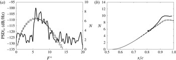
(a) Experimental spectra of
 $v^{\prime }$
and linear stability theory (LST)
 $N$
factors at
 $x/c=0.85$
. (b) Experimental and LST
 $N$
factors for
 $F^{+}=6$
. Dashed lines indicate uncertainty intervals for LST predictions. Experimental data pertain to the baseline case.

For validation purposes, figures 11(a,b) present a comparison between linear stability theory (LST) predictions and the baseline experimental data for the frequencies of the amplified disturbances and the amplification factors of the most amplified disturbances (
 $N(x)=\ln (A(x)/A(x_{ref})$
, where
 $A$
is the disturbance amplitude and
 $x_{ref}$
is the reference location). As discussed by Boutilier & Yarusevych (Reference Boutilier and Yarusevych2013), LST predictions are known to be sensitive to the effects of measurement noise in the mean velocity fields. Here, the uncertainty in LST predictions is estimated by propagating the estimated experimental uncertainty through stability calculations. The obtained uncertainty bounds are marked by the shaded regions in figure 11, and the degree of variation in stability predictions due to experimental error is in agreement with that reported in Boutilier & Yarusevych (Reference Boutilier and Yarusevych2013). In figure 11(a), a spectrum of wall-normal velocity fluctuations shows the amplification of disturbances within
 $5\leqslant F^{+}\leqslant 10$
, with the highest energy content associated with disturbances at
 $F^{+}\approx 6$
. The overlaid plot of
 $N$
factors shows that this frequency range falls within the unstable frequency band from LST and the frequency of the most amplified disturbances matches the LST predictions to within experimental uncertainty. It should be noted that the exact comparison of experimental amplification factors and those from LST results cannot be performed since the disturbances in the experiment can only be detected well downstream of the neutral stability point, where they reach measurable amplitudes. Thus, following the conventional approach used in stability investigations (Schmid & Henningson Reference Schmid and Henningson2001), the amplification factors are matched at a reference location (
 $x_{ref}/c\approx 0.805$
), where the experimentally measured disturbance amplitudes reach
 $0.005U_{0}$
. The experimental data were bandpass filtered at
 $F^{+}=6\pm 0.2$
to compute amplification factors corresponding to the most amplified disturbances. As shown in figure 11(b), the experimental results capture well the initial nearly exponential growth of the disturbances and are in good agreement with the LST predictions in this region. As the growth of disturbances begins to saturate, the agreement with LST deteriorates since nonlinear effects become significant. Similar results were also obtained for the forced cases, confirming that LST analysis can be used to predict stability characteristics of the separation bubbles observed in the present study.
LST analysis on the LSB for different forcing frequencies (
 $f^{+}$
). (a) Growth rate contours. Location of maximum growth rate (
 $-\unicode[STIX]{x1D6FC}_{i}^{min}$
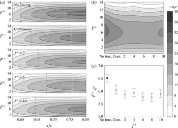
) (solid white line), location of separation (dashed black line) and mid-location between separation and maximum bubble height (dashed white line). (b) Growth rate as function of forcing frequency at the mid-location between separation and maximum bubble height. (c) Frequency of most unstable mode (maximum growth rate) at mid-location between separation and maximum bubble height.

The effect of forcing on stability characteristics of the separation bubble is first examined in figure 12 for the constant amplitude forcing applied at different frequencies, with the excitation parameters matching those presented in figure 5. Figure 12(a) presents the contours of the local growth rate of disturbances (
 $-\unicode[STIX]{x1D6FC}_{i}$
), with negative values associated with convectively amplified disturbances, in line with the spatial formulation of LST used in this study. For the baseline case, the stability results show that the frequency of the most amplified disturbances (traced by a solid white line) increases gradually downstream of separation (dashed black line), levelling off at
 $F^{+}=6$
by the mid-point between separation and maximum bubble height position (white dashed line), where the amplification of disturbances at this frequency is first detected in the corresponding experimental measurements (figure 9). When forcing is applied, the growth rates associated with the most unstable disturbances in the separation bubble diminish notably but the corresponding frequencies are not affected to the same degree. This is illustrated in figures 12(b) and 12(c), which compare the growth rates and the frequencies of the most unstable disturbances, respectively, at the locations marked by the white dashed lines in figure 12(a). Figure 12(b) shows that the introduction of artificial disturbances leads to a significant decrease in the growth rate, proportional to the relative decrease in the size of the separation bubble produced by the forcing (figure 6). Specifically, at this streamwise location, the maximum normalised growth rate for the baseline case is
 $-\unicode[STIX]{x1D6FC}_{i}c\approx 30$
; whereas, that for the forced case at
 $f^{+}=6$
decreases to about 20. The frequency of the most unstable disturbances also decreases (figure 12) since the bubble size is affected by the forcing. It reaches a minimum at approximately
 $f^{+}=6$
, where the most amplified frequency is reduced from
 $F^{+}|_{\unicode[STIX]{x1D6FC}_{i}^{min}}=6.65$
to
 $F^{+}|_{\unicode[STIX]{x1D6FC}_{i}^{min}}=5.75$
. Thus, the fact that the most significant effect on separation bubble was observed at the frequency matching that of the most amplified disturbances in the baseline flow is attributed to the relatively small change in the most unstable frequency produced by forcing at this amplitude.
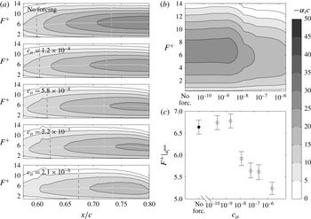
LST analysis on the LSB for different forcing amplitudes (
 $c_{\unicode[STIX]{x1D707}}$
). (a) Growth rate contours. Location of maximum growth rate (
 $-\unicode[STIX]{x1D6FC}_{i}^{min}$
) (solid white line), location of separation (dashed black line) and mid-location between separation and maximum bubble height (dashed white line). (b) Growth rate as function of forcing amplitude at the mid-location between separation and maximum bubble height (for consistency with the logarithmic scale no forcing has been placed at
 $c_{\unicode[STIX]{x1D707}}=10^{-11}$
). (c) Frequency of most unstable mode (maximum growth rate) at mid-location between separation and maximum bubble height.

Figure 13 illustrates the effect of forcing amplitude on stability characteristics of the laminar separation bubble for the fixed excitation frequency of
 $f^{+}=6$
. It can be seen that no substantial changes in the growth rate or the associated frequency of the most amplified disturbances are attained at low excitation amplitudes (figure 13
b,c), with no significant changes to the mean bubble characteristics produced at these excitation conditions (figure 8). However, as the forcing amplitude exceeds
 $c_{\unicode[STIX]{x1D707}}=2\times 10^{-9}$
, it leads to changes in the mean bubble parameters (figure 8) and, hence, the stability characteristics (figure 13). Specifically, as the forcing amplitude increases above this threshold, both the maximum growth rate and the associated frequency decrease (figures 13
b–c), following the associated decrease in the bubble length and height (figure 8
b). At the highest excitation amplitudes examined, the frequency of the most amplified disturbances is reduced by approximately 20 % compared to the baseline case (no forcing).
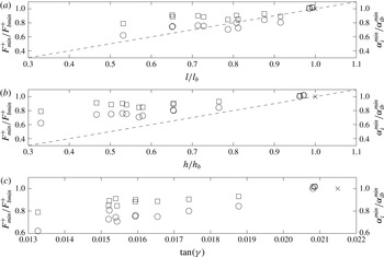
A comparison of the flow measurements and stability results suggests that the most notable changes in stability characteristics correspond to the cases when artificial disturbances produce the most significant changes to the mean size of the separation bubble. This is illustrated in figures 14(a) and 14(b), which show the variation of the maximum growth rates and the associated frequencies with bubble length and height, respectively. The results demonstrate that both the frequency and the growth rate of the most amplified disturbances decrease as the size of the bubble decreases. A similar effect of artificial forcing has also been observed in the numerical simulations of Marxen & Rist (Reference Marxen and Rist2010), Marxen & Henningson (Reference Marxen and Henningson2011) and Marxen et al. (Reference Marxen, Kotapati, Mittal and Zaki2015) on a flat plate geometry subjected to an adverse pressure gradient, and was attributed to the mean flow deformation. It can be seen from figure 14(a,b) that the reduction in the size of the separation bubble (either length or height) compared to the baseline case produces a decrease in the relative maximum growth rate and the most amplified frequency. However, the growth rate decreases more rapidly in comparison to the frequency, with the relative decreases in the growth rate being, on the average, double that in the frequency for a given reduction in the bubble size.
Frequency (▫) and growth rate (○) of most amplified disturbances as a function of (a) bubble length, (b) bubble height and (c) angle of separation (
 $\unicode[STIX]{x1D6FE}$
) for all tested cases. All values are normalised with the respective quantities pertaining to the no forcing case (
 $\times$
). Dashed lines correspond to a
 $45^{\circ }$
slope.

The observed weaker effect of mean flow deformation on the frequency of the most amplified disturbances in the separated shear layer is consistent with the recent results of Marxen et al. (Reference Marxen, Kotapati, Mittal and Zaki2015), who numerically modelled separation bubble control with a synthetic jet. Similar to the earlier conclusion made in the present study, this reduced sensitivity of the unstable frequency to the changes in the mean bubble size due to excitation explains why the optimum excitation effect has been observed in other flow control studies when periodic flow excitation was applied at the frequency of the most amplified disturbances in the base flow. For example, Yarusevych, Kawall & Sullivan (Reference Yarusevych, Kawall and Sullivan2006a ) and Yarusevych, Sullivan & Kawall (Reference Yarusevych, Sullivan and Kawall2006b ) observed that the optimal frequency of external acoustic excitation and that of the most amplified disturbances in the base flow agree to within approximately 10 %.
It can be inferred from the analysis of the present results that the diminishment of the bubble is produced due to the amplification of artificial disturbances in the separated shear layer, which is governed by the underlying stability of the mean flow. Marxen et al. (Reference Marxen, Kotapati, Mittal and Zaki2015) also attributed the most effective control strategy in their numerical simulation to a convective instability in the separated shear layer, although other instability mechanisms were also observed. The quantitative flow visualisations in figure 10 suggest that the mean flow reattachment is attained due to the enhanced entrainment of momentum by the shear layer vortices, shed in the aft portion of the bubble at the frequency of the most amplified disturbances. Thus, the upstream advancement of the mean reattachment by means of artificial two-dimensional disturbances requires that such disturbances attain critical amplitude and produce shear layer roll-up earlier upstream, which is observed in the present measurements (figures 5 and 10). Given the decrease in maximum growth rates with decreasing the size of the bubble, revealed by the stability analysis (figure 14 a,b), the implication here is that the disturbances attain higher amplitudes at the same locations within the bubble (figure 7) due to the higher initial amplitudes produced by the actuator. The increased stability of smaller bubbles is likely responsible for the gradual reduction in the mean deformation effect with the decrease of the separation bubble size seen in figure 14(a,b). Specifically, on the average, as the bubble size diminishes, the relative change in stability characteristics gradually decreases.
The observed effect of mean bubble deformation on stability characteristics is speculated to be dependent primarily on the distance between the separated shear layer and the wall. Dovgal et al. (Reference Dovgal, Kozlov and Michalke1994) and Diwan & Ramesh (Reference Diwan and Ramesh2009), using synthetic mean velocity profiles and experimental data, respectively, concluded that this is one of the main parameters affecting separated shear layer stability characteristics. As an approximation, the distance between the separated shear layer and the wall in a separation bubble can be represented by the angle between the dividing streamline and the wall (
 $\unicode[STIX]{x1D6FE}$
) in the wall-attached coordinates, with
 $\tan (\unicode[STIX]{x1D6FE})=h/l$
. The variation of maximum growth rates of disturbances and the associated frequencies with
 $\tan (\unicode[STIX]{x1D6FE})$
is presented in figure 14(c). The results demonstrate that the decrease in the separation angle leads to the decrease in the associated stability characteristics. The distance between the wall and the core of the separated shear layer can be approximated more precisely using a displacement thickness (Boutilier & Yarusevych Reference Boutilier and Yarusevych2012). At the same time, integral boundary layer characteristics at separation are also often used as characteristics length scales (Boiko et al.
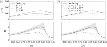
Reference Boiko, Grek, Dovgal and Kozlov2002). Since the momentum thickness does not vary substantially in the fore portion of the separation bubble, the shape factor (
 $H$
) can be used as a suitable dimensionless parameter, which also allows a comparative analysis with other studies. The effect of excitation on these integral parameters is illustrated in figure 15, which shows the expected decrease in both the momentum thickness and the shape factor proportional to the effect of excitation on the separation bubble size.
Displacement thickness (
 $\unicode[STIX]{x1D6FF}^{\ast }$
) and shape factor
 $(H)$
as function of (a) forcing frequency and (b) forcing amplitude. Shaded grey areas denote uncertainty intervals.

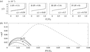
Comparison of the no forcing case (solid lines) at four streamwise locations to the Blasius (dashed line) profile at
 $x/c=0.59$
and hyperbolic tangent profile (dotted dashed line) at
 $x/c=0.735$
. (a) Streamwise velocity profiles and (b) LST growth rates.

A prominent effect of shape factor on stability characteristics is depicted in figure 16 for the no forcing case examined in the present investigation. The results demonstrate that both the maximum growth rate and the corresponding frequency decrease and the band of unstable frequencies narrows with decreasing shape factor. In figure 16(b), dispersion relations representative of the free shear layer (hyperbolic tangent profile) and the attached Blasius boundary layer are also plotted for comparison with the corresponding profiles shown in figure 16(a). It can be seen that the stability characteristics of the laminar separation bubble lie between the limiting cases of the attached, zero pressure gradient boundary layer and the free shear layer.
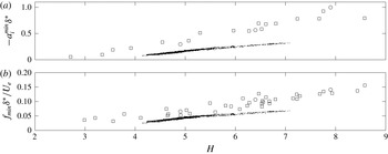
(a) Maximum growth rate as function of the LSB shape factor for all tested cases and (b) most unstable frequency as function of the LSB shape factor for all tested cases. Scatter points are plotted for locations between separation and mid-point between separation and maximum height. For comparison, cases pertaining to the studies of Boutilier & Yarusevych (Reference Boutilier and Yarusevych2012) (○) and LeBlanc, Blackwelder & Liebeck (Reference LeBlanc, Blackwelder and Liebeck1989) (▫) are shown.

Figure 17 compares the variation of non-dimensional maximum growth rate and the frequency of the most amplified disturbances with the shape factor. The figure also includes the data from other studies involving laminar separation bubbles on different aerofoils, where relevant parameters could be extracted. The results show that using the displacement thickness as the reference length scale effectively collapses each data set on a linear trend. The observed data scatter lies within experimental uncertainty in the relevant parameters (e.g. figures 12(c), 13(c) and 15). This is particularly significant considering that the results from Boutilier & Yarusevych (Reference Boutilier and Yarusevych2012) pertain to a constant Reynolds number but different angles of attack, while both of these parameters were varied over a relatively wide range in LeBlanc et al. (Reference LeBlanc, Blackwelder and Liebeck1989). Although there are deviations between the individual linear fits, there is a clear increase in the growth rate with increasing the shape factor for different geometries and flow characteristics, and the proposed functional dependence of stability characteristics shows good robustness for a given aerofoil profile. This implies that, for a given geometry, the shape factor effectively governs the non-dimensional stability characteristics of the separated shear layer.
3.2 Transient response
The discussed relation between the development of artificial disturbances, stability characteristics of the bubble, and the attendant mean flow deformation obtained for the steady state cases highlights the importance of considering the transient flow development that ensues when controlled disturbances are either introduced or removed from the flow. The transient behaviour of the separation bubble is also of interest from the perspective of flow control development and implementation. Since disturbances affect the bubble dynamics and mean parameters, stability characteristics are expected to change when artificial disturbances are introduced or removed from the flow, thereby affecting the transient flow development until a quasi-steady state is reached. In addition, the transient development can be anticipated to depend on the initial mean flow state and, consequently, is likely to differ depending on whether artificial disturbances are introduced to the flow or removed from it. The transient dynamics of the separation bubble associated with the introduction of artificial disturbances and the termination of forcing is examined in this section using the case of excitation at
 $f^{+}=6$
and
 $c_{\unicode[STIX]{x1D707}}=5.8\times 10^{-8}$
(
 $V_{pp}=3.5$
kV).
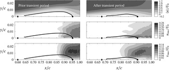
Time-averaged streamwise velocity field (
 $\langle u\rangle$
), fluctuating streamwise (
 $u_{rms}$
) and wall-normal (
 $v_{rms}$
) velocity fields prior to and after the period of transient response to the introduction of forcing (
 $f^{+}=6$
,
 $c_{\unicode[STIX]{x1D707}}=5.79\times 10^{-8}$
). Time-averaged dividing streamline (thick solid line), mean separation point (
 $\blacklozenge$
) and mean reattachment point (●).

Figure 18 compares time-averaged flow field characteristics for the baseline case and the excited flow, which represent approximate quasi-steady state limits for the investigated transient separation bubble dynamics. As discussed earlier, the introduction of artificial disturbances results in higher velocity fluctuations being attained earlier upstream, leading to earlier and more coherent shear layer roll-up. As a consequence, both the length and height of the separation bubble are reduced. However, it can be seen from the root-mean-square fields that stronger velocity fluctuations, particularly in wall-normal velocity, are produced in the aft portion of the separation bubble in the baseline case. Notwithstanding the increased amplitude of incoming disturbances during the excitation, it is striking to note that the location of the maximum height of the bubble approximately corresponds to the same level of maximum velocity fluctuations in both the forced and unforced bubble. At the same time, for the excited flow, the magnitude of maximum vertical velocity fluctuations induced by shear layer vortices in the aft portion of the bubble is reduced due to the proximity of the wall.
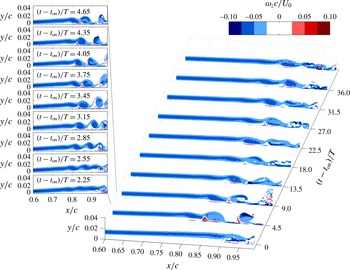
Evolution of spanwise vorticity (
 $\unicode[STIX]{x1D714}_{z}$
) in the transient period after initiation of forcing (on). Inset indicates a more detailed evolution in the period
 $2.25<t-t_{on}<4.65$
.

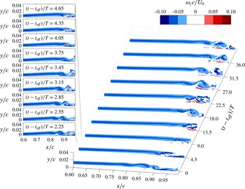
Figures 19 and 20 present sequences of vorticity snapshots spanning the transients encountered after the introduction of excitation and after its removal, respectively. The results in figure 19 confirm that introducing the artificial disturbances moves the roll-up location upstream and, initially, produces much stronger rollers, as can be seen at
 $(t-t_{on})/T=4.5$
and in the inset detailed sequence. The roll-up location then moves downstream, and the quasi-steady shedding is established at approximately
 $(t-t_{on})/T\approx 20$
. When the excitation is removed (figure 20), the shear layer roll-up moves downstream, moving outside of the field of view at
 $(t-t_{off})/T\approx 9$
. The bubble effectively bursts, which is followed by a gradual upstream advancement of the roll-up location that converges on a quasi-steady state similar to that observed in the baseline case without excitation at
 $(t-t_{on})/T\approx 30$
.
Evolution of spanwise vorticity (
 $\unicode[STIX]{x1D714}_{z}$
) in the transient period after cessation of forcing (off). Inset indicates a more detailed evolution in the period
 $2.25<t-t_{on}<4.65$
.

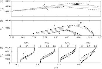
Transient response of the LSB topology to initiation of forcing. All quantities are based on a sliding average spanning 2.5 global convective time units. (a) Successive loci of
 $\unicode[STIX]{x1D6FF}^{\ast }$
(grey solid line) and (b) successive dividing streamlines (black solid line) are spaced with 0.875 convective time units. Start (thick dashed lines) and end (thick dash-dotted lines) of the transient response. Probe locations P1 (○) and P2 (▫) located at streamwise location of maximum bubble height. Trajectory of maximum
 $\unicode[STIX]{x1D6FF}^{\ast }$
during transient period (thick solid black line). (c) Successive streamwise velocity profiles (identical notation as in (a)). Black arrows denote increasing time.

The transient response of the LSB is investigated further by obtaining statistical estimates of flow characteristics via a sliding average within a time window of 2.5 global convective time scales in width (
 $2.5c/U_{0}$
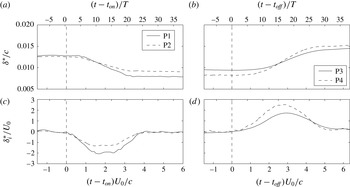
). This approach allows elucidating global temporal changes while reducing the random noise in the data. The width of the sliding window is selected as a compromise between the temporal smoothing and noise reduction; nevertheless, the overall trends were verified to be largely insensitive to the width of the window within a band from 1 to 4 convective time scales. Figure 21 presents the variation of the displacement thickness and dividing streamline when the excitation is introduced. Changes in the mean streamwise velocity profiles are also shown in the figure. Here, the presented properties evolve from those in the unforced bubble (marked by dashed lines) to the quasi-steady bubble attained by continuous excitation (dash-dotted line) in time increments of
 $0.875c/U_{0}$
. The local displacement thickness is representative of the averaged height of the convectively amplified wave packet in the separated shear layer, with the location of the maximum displacement thickness (solid line in figure 21
a) approximately marking the onset of shear layer roll-up (cf. figure 19). Examination of the results in figure 21 suggests that the bubble does not respond monotonically to the onset of excitation. Shortly after the onset of excitation (
 $t-t_{on}\lesssim 0.9c/U_{0}$
), relatively small changes are observed within the bubble. This is followed by the rapid advancement of the roll-up location upstream (figure 21
a) accompanied by the upstream advancement of the mean reattachment location and the overall reduction in the size of the separation bubble (figure 21
b). After the bubble attains a minimum size, it expands back to the quasi-steady state characteristics representative of continuous excitation, in agreement with the movement of the roll-up location in figure 19.
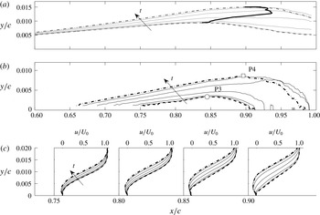
Figure 22 presents changes in the same variables as those shown in figure 21 for the transient case ensuing when the excitation is stopped. The initial bubble characteristics prior to the onset of the transient are marked by dashed lines, while those established after the transient period are identified with dash-dotted lines. As in the case of the transient observed after the introduction of artificial disturbances, the bubble undergoes non-monotonic topological changes between the two quasi-steady states. Initially for (
 $t-t_{off}\lesssim 1.5c/U_{0}$
), relatively small changes are observed in the parameters. This is followed by a rapid downstream movement of the roll-up location (figures 20 and 22
a), with the mean bubble growing both in length and in height (figure 22
b). During the second half of the transient process, the mean bubble reaches its maximum extent and then contracts to the quasi-steady state sustained in the absence of excitation.
Transient response of the LSB topology to cessation of forcing. Identical notation to figure 21.

A more close examination of temporal changes during these two transient processes is performed by considering time histories of window-averaged displacement thickness, and local velocity fluctuations. The results are presented in figures 23 and 24 using two probe locations identified in figures 21 and 22, which correspond to the streamwise location of the maximum mean bubble height for the initial and final configurations in each of the two transient cases respectively. The temporal changes are characterised on two time scales: one relative to the global convective time scale (
 $c/U_{0}$
), and another relative to the average shedding period of the shear layer vortices (
 $T$
), which effectively coincides with the forcing period. Figures 23(a) and 23(b) compare temporal variations in the window-averaged displacement thickness and its temporal rate of change, respectively. For the case when the excitation is turned on, the transient process lasts approximately 4 global convective time units (
 $4c/U_{0}$
) or approximately 23 shedding periods. When the excitation is turned off, the duration of the transient process increases by about 45 %, lasting approximately
 $5.5c/U_{0}$
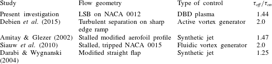
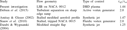
or 33 shedding periods. A similar disparity in the duration of the transients associated with the control of highly separated shear flows has been reported in some previous studies summarised in table 2. For a variety of flow configurations, the ratio of the transient duration when the excitation is turned off to that when the excitation is introduced (
 $\unicode[STIX]{x1D70F}_{off}/\unicode[STIX]{x1D70F}_{on}$
) ranges from 1.25 to 2, with
 $\unicode[STIX]{x1D70F}_{off}/\unicode[STIX]{x1D70F}_{on}\approx 1.44$
in the present study. Although it was speculated that the transient flow development is related to mean flow stability to the introduced perturbations (Darabi & Wygnanski Reference Darabi and Wygnanski2004), this has not been investigated in detail to this point.
Comparison of previous studies involving transient flow development in control of separated flows.
Inspection of figure 23 suggests that significant changes in bubble characteristics begin at earlier times when the excitation is introduced, compared to the case when the excitation is turned off. In figure 23(b), the maximum rate of change in
 $\unicode[STIX]{x1D6FF}^{\ast }$
is obtained approximately 10 shedding cycles after the onset of excitation and a nearly constant maximum rate of change is sustained for over 5 shedding cycles. When the excitation is turned off, a comparable maximum rate of change in
 $\unicode[STIX]{x1D6FF}^{\ast }$
is attained after approximately 15 cycles, followed by a gradual decay in the slope. Consequently, a shorter transient duration is attained in the former case.
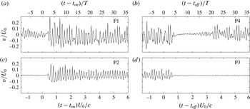
The time traces of the vertical velocity in figure 24 provide added insight into the temporal changes in the bubble. The traces show that the aft portion of the bubble does not encounter appreciable changes for a few shedding periods after the onset of the excitation, with the time delay, on the average, representing the convective time it takes the introduced disturbances at the actuator position to reach the probe locations. At the onset of the excitation, the initial pulse produces a strong perturbation seen in the traces from the probes at
 $(t-t_{on})/T\approx 2.5$
, with the amplitude of subsequent periodic fluctuations decaying gradually. This suggests a much stronger amplification of the leading disturbances at the onset of excitation, which is also seen in figure 19. When the excitation is turned off, the amplitude of fluctuations begins to decay at
 $(t-t_{off})/T\approx 4$
, implying that the higher-amplitude velocity fluctuations induced by the forcing are sustained for about 4 cycles after the forcing is turned off (2 cycles longer than the delay expected based on the propagation speed of disturbances).
(a) Evolution of boundary layer displacement thickness in the transient period after initiation of forcing (on) and cessation of forcing (off) and (b) rate of change of
 $\unicode[STIX]{x1D6FF}^{\ast }$
in the respective transient periods. All values are based on a sliding average spanning 2.5 convective units. Vertical dashed line denotes start of the transient period. The probe locations are indicated in figures 21(b) and 22(b).


Evolution of growth rate pertaining to mode frequency of
 $f^{+}=6$
in the transient period after (a) initiation of forcing (on) and (b) cessation of forcing (off). Data are calculated at the mid-location between separation and maximum height of the baseline bubble (
 $x/c\approx 0.73$
).

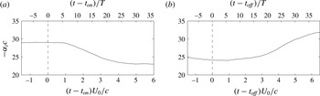
Clearly, the observed transient bubble dynamic behaviour is related to the development of the shear layer disturbances. Additionally, it follows from the previous discussion that the amplification rate of the disturbances in the separated shear layer is expected to change during the transient. To shed light on the physical mechanism behind the transient flow development associated with the introduction and removal of harmonic excitation, it is instructive to consider the changes in the stability characteristics of the separated shear layer. Figure 25 shows the variation of the growth rate associated with the average shear layer shedding frequency, which also matches the excitation frequency. The results are obtained based on the linear stability analysis of the sliding averages of the velocity fields within the transient, and serve as a first-order approximation for the overall variation in the growth rate. The data confirm that substantial changes in the growth rate occur during the transient. Specifically, when the excitation is introduced (figure 25 a), the bubble becomes more stable and, as its length and height are gradually reduced, the growth rate diminishes. The opposite trend is seen for the case when the excitation is turned off (figure 25 b).
These changes in stability characteristics provide insight into the attendant transient flow development. In particular, at the moment of introduction of the excitation, the bubble has not yet reacted and complies to the stability characteristics of the unforced flow. The bubble is rather unstable and hence the injection of higher amplitude initial disturbances at the most unstable frequency leads to a much earlier shear layer roll-up and the formation of a strong train of initial shear layer vortices (figure 19). This leads to a significant increase in the entrainment of higher momentum fluid from the outer flow, causing the bubble to contract rapidly (figures 21 and 23). However, as the bubble contracts, the flow becomes more stable and the amplification of the following disturbances reduces. As such, the smallest bubble state cannot be sustained due to the lower amplification rates experienced by the subsequent disturbances and consequently lower momentum entrainment. As a result, the bubble expands in the second part of the transient (figure 21) to settle on a quasi-steady configuration. In contrast, for the transient associated with the removal of excitation (figure 25 b), the bubble is more stable at the onset of the transient compared to the bubble forming in the absence of forcing. When the excitation that sustains such a state of the bubble is removed, the higher-amplitude harmonic disturbances are replaced by a broader spectrum of lower-amplitude natural perturbations, leading to much weaker velocity fluctuations being attained in the aft portion of the bubble (figure 20). As a result of the weakened momentum entrainment, the same mean bubble topology can no longer be maintained and the bubble effectively bursts (figure 20), i.e. the size of the bubble increases rapidly (Marxen & Henningson Reference Marxen and Henningson2011). Although the shear layer in the burst bubble becomes more unstable, the lower initial amplitude of the disturbances leads to a delayed shear layer roll-up. The bursting also significantly weakens the upstream feedback loop, as hypothesized by Dovgal et al. (Reference Dovgal, Kozlov and Michalke1994) and Boiko et al. (Reference Boiko, Grek, Dovgal and Kozlov2002), where pressure fluctuations produced due to the shedding of the shear layer vortices in the aft portion of the bubble feed back upstream and influence the initial amplitude of the disturbances. The existence of such a feedback is supported by studies on aerofoil tonal noise (e.g. Desquesnes, Terracol & Sagaut Reference Desquesnes, Terracol and Sagaut2007), since periodic passage of shear layer vortices over the trailing edge leads to relatively strong harmonic acoustic emissions establishing a stronger upstream feedback loop and locking shear layer disturbances more closely to the shedding frequency (Pröbsting & Yarusevych Reference Pröbsting and Yarusevych2015). While the influence of such tonal emissions is insignificant compared to that of artificial disturbances for the excited flow, it can alter the characteristics of the naturally developing bubble (Pröbsting & Yarusevych Reference Pröbsting and Yarusevych2015). Once the shedding resumes, the feedback loop is re-established, and the bubble contracts to a quasi-stable state (figures 20 and 22). Contrasting the two transient cases in this context suggests that the different stability characteristics of the initial state of the bubble, coupled with the importance of the upstream feedback loop in the absence of excitation, are largely responsible for the significant differences in the duration of the transients observed.
(a) Snapshots of wall-normal velocity (
 $v$
) in the transient period after initiation of forcing. (b) Evolution of integrated wall-normal velocity (
 $\int v\,\text{d}y$
) in the transient period after forcing initiation (on). Dotted dashed lines correspond to location of labelled vortices.

(a) Snapshots of wall-normal velocity (
 $v$
) in the transient period after cessation of forcing. (b) Evolution of integrated wall-normal velocity (
 $\int v\,\text{d}y$
) in the transient period after forcing cessation (on). Dotted dashed lines correspond to location of labelled vortices.

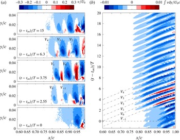
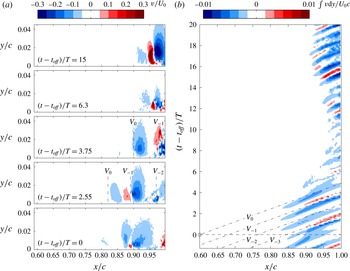
The spatio-temporal evolution of the vortices during the two transients is examined more quantitatively in figures 26 and 27, where the vortices are traced using the wall-normal velocity. More specifically, the snapshots in figures 26(a) and 27(a) pertain to instantaneous wall-normal velocity contours while the trace maps in figures 26(b) and 27(b) are constructed using the integral of wall-normal velocity in the wall-normal direction (
 $\int v\,\text{d}y$
). The integral quantity (
 $\int v\,\text{d}y$
) serves as a measure of the intensity of wall-normal velocity fluctuations induced by the passing structures at a given streamwise location. As expected, the periodically shed vortices produce a distinct periodic train of positive and negative velocity regions, shown in figure 26(a), where approximate locations of individual vortical structures of interest are marked by dashed-doted lines for illustration purposes. Respectively, the produced convective ridges between minima and maxima in integral wall-normal velocity, marked by the dashed-doted lines in figure 26(b), follow the streamwise evolution of the structures. The ridge that intersects
 $t=0$
corresponds to the vortex that originates from a disturbance produced at the actuator location (
 $x/c=0.6$
) at the onset of the transient. For the transient encountered after the excitation is introduced (figure 26), it can be seen that the vortex produced by the first pulse (
 $V_{0}$
) is notably stronger, compared to the structures formed prior to the onset of actuation. However, the growing perturbation introduced by the first pulse induces a stronger preceding vortex (
 $V_{-1}$
), compared to the amplified background disturbances. This stronger vortex reaches the mean reattachment location of the initial mean bubble (
 $x/c\approx 0.95$
) at
 $t-t_{on}\approx 3T$
, which corresponds to the time when measurable changes in bubble characteristics begin in figure 23. The vortices
 $V_{0}$
,
 $V_{1}$
,
 $V_{2}$
,
 $V_{3}$
and
 $V_{4}$
, which are shed between the onset of excitation and the time vortex
 $V_{-1}$
starts to affect the initial trajectory of the separated shear layer, are characterised by similar magnitude of vertical velocity fluctuations. As these structures travel downstream and enhance the entrainment of higher momentum fluid in the aft portion of the bubble within
 $3T\lesssim t-t_{on}\lesssim 9T$
, significant changes in the bubble characteristics are observed (figure 23). As a result of the ensuing changes to the bubble and the associated decrease in the growth rate (figure 25
a), the strength of the subsequent vortices gradually decreases (figure 26), with a quasi-steady state reached at
 $t-t_{on}\approx 20T$
corresponding to the time when the bubble characteristics stop changing in figure 23.
Figure 27 illustrates the spatio-temporal development of the shear layer vortices during the transient associated with the cessation of excitation. The vortex labelled
 $V_{0}$
is the structure that develops from the last pulse of the actuator, while
 $V_{-1}$
,
 $V_{-2}$
are preceding vortices. It can be seen that, in contrast to the transient associated with the introduction of the forced disturbance, where a significant upstream effect of the first controlled disturbance resulted in the formation of a stronger preceding vortex (
 $V_{-1}$
in figure 26), a much weakened effect of the last strong pulse (
 $V_{0}$
) on the following unforced disturbance is observed in figure 27. The considerably weaker disturbance following the last controlled perturbation stems from the significantly increased stability of the excited flow (figure 25
b). The direct consequence of this effect is the delayed temporal response of the flow to the cessation of forcing, compared to the initiation of forcing. Specifically, in figure 27, the last strong vortex interacting with the reattachment region is
 $V_{0}$
at
 $t-t_{off}\approx 4T$
and the first disturbances of significantly lower amplitude reach this region one shedding period later at
 $t-t_{off}\approx 5T$
. In figure 26, the first high amplitude vortex that interacts with the reattachment region is
 $V_{-1}$
at
 $t-t_{off}\approx 3T$
. As such, the difference of two shedding periods in arrival time of the leading altered-amplitude disturbances between the two cases corresponds directly to the difference between the times significant changes are observed in figure 23. Following
 $V_{0}$
, the results in figure 27 show a dramatic decrease in the magnitude of vertical velocity fluctuations, with no sign of roll-up observed within the field of view. This confirms that the bursting of the bubble is produced because the much smaller background disturbances remaining after the cessation of excitation reach insufficient amplitudes to sustain the initial state of the bubble. As discussed previously, this is related to the lower growth rate experienced by the disturbances in this bubble configuration (figure 25
b).
4 Conclusions
The present study examined experimentally both the steady and transient response of a laminar separation bubble to two-dimensional, periodic disturbances. The bubble was generated on a NACA 0012 aerofoil in an open-jet wind tunnel facility at
 $Re_{c}=130\,000$
and
 $\unicode[STIX]{x1D6FC}=2^{\circ }$
, and the flow development was assessed by means of time-resolved, two-component PIV. The controlled disturbances were introduced using a DBD plasma actuator installed upstream of the mean laminar boundary layer separation location. For steady excitation, the effect of excitation amplitude and frequency on the separated shear layer transition process and the spatio-temporal dynamics of the separation bubble was examined. The transient flow dynamics encountered at the onset of excitation and after its removal was also investigated. A linear stability analysis was employed to relate the observed flow development to shear layer stability characteristics and provide insight into the attendant bubble dynamics.
The results show that separation bubble development is largely governed by the formation of shear layer roll-up vortices. These structures, which originate from the amplification of unstable disturbances in the separated shear layer, form in the aft portion of the bubble and facilitate the entrainment of higher momentum fluid from outer flow towards the near-wall region, inducing flow reattachment in the mean sense. In the presence of natural background disturbances, the average shedding frequency of these structures matches the frequency of the most amplified disturbances in the separated shear layer, and notable temporal variations in the shedding frequency and wavelength of the structures occur due to the inherent minute temporal variations in the background disturbance environment. The shear layer vortices begin to break down in the vicinity of mean reattachment, with weakly coherent structures advecting into the redeveloping turbulent boundary layer. When artificial harmonic disturbances are introduced at a frequency sufficiently close to the most unstable frequency, the transition process locks onto the excitation frequency, significantly increasing the coherence of the shed vortices. This also advances the roll-up location upstream and leads to the formation of more coherent structures that propagate farther downstream before breaking up to smaller scales. Consequently, the mean reattachment location advances upstream and the overall length and height of the separation bubble are reduced. The effect is most pronounced when the excitation is applied at the most unstable frequency and diminishes progressively as the excitation frequency deviates towards higher or lower values. When the excitation is applied above a minimum threshold amplitude, increasing excitation amplitude enhances the effect on the bubble, with bubble length and height decreasing nearly exponentially with increasing momentum coefficient.
Linear stability analysis results demonstrate that changes in mean bubble topology induced by the excitation lead to notable changes in the flow stability characteristics. In particular, the maximum growth rate and the most amplified frequency decrease with decreasing bubble size, with the decrease in the former parameter being more significant. The reduction in growth rate is nearly linearly proportional to the reduction in bubble length, with a decrease of approximately 40 % in bubble length decreasing the growth rate magnitude by approximately 35 %. The associated reduction in the most amplified frequency is more moderate, as the same change in bubble length reduces the most amplified frequency by approximately 20 %. The observed decrease in the growth rate magnitude indicates that the upstream advancement of the shear layer roll-up and, ultimately, the reduction in the size of the separation bubble by artificially introduced disturbances is attributed solely to the increase in the initial amplitude of perturbations. While being more moderate by comparison, the associated reduction in the frequency of the most amplified disturbances is of interest for the optimisation of active flow control strategies, where a proportional adjustment of the controller frequency can improve its efficiency.
The analysis of stability characteristics of laminar separation bubbles has shown that the observed changes in bubble stability are related primarily to the changes in the integral boundary layer characteristics. A new correlation has been proposed, revealing that both the growth rate and the most amplified frequency scale with the shape factor. In particular, the non-dimensional growth rate and frequency of the most amplified disturbances increase nearly linearly with increasing shape factor. The effect is argued to be related to the influence of the wall proximity on the development of shear layer disturbances, with the limiting cases for both stability parameters, i.e. their minimum and maximum limits, correlating well with the characteristics of the attached boundary layer and free shear layer, respectively. Applying the proposed correlation to the available data sets from other studies on different aerofoil geometries verified the universality of the observed governing role of the shape factor on stability characteristics, although fit parameters vary between different experiments.
The investigation of the transient response of the separation bubble has revealed significant differences in the duration and dynamics of the transient flow development between the transients associated with the introduction of excitation and its removal. In the former case, the duration of the transient is approximately 40 % shorter, lasting approximately 23 shedding cycles. The differences in the progression of the transients have been shown to be governed by differences in the stability characteristics of the separated shear layer. When the excitation is introduced into the unforced separation bubble, the bubble is highly unstable and the artificial disturbances are strongly amplified in the separated shear layer, leading to the earlier formation of much stronger shear layer vortices. The passage of these structures over the aft portion of the bubble enhances the entrainment of momentum into the near-wall region, resulting in a rapid contraction of the bubble. However, as the bubble contracts, it becomes more stable and the subsequent artificial disturbances undergo weaker amplification, producing progressively weaker roll-up vortices. The transient process continues until the bubble settles on a quasi-steady forced configuration. In contrast, when the excitation of the forced bubble is ceased, the initial state of the bubble is more stable compared to that of the unforced bubble. As much weaker natural disturbances enter the separated shear layer, they undergo a relatively slow amplification leading to a significant delay in separated shear layer roll-up. The ensuing sudden interruption of strong vortex shedding impedes the momentum entrainment required to sustain the forced mean bubble configuration, and the bubble bursts. This also disrupts the upstream feedback loop, which is significant for the unforced bubble development and further delays the re-establishment of the quasi-steady configuration of the unforced bubble. As a consequence, the transient duration increases significantly compared to that observed when the excitation is introduced. The observed differences are of particular importance for active flow control implementation and the uncovered relation between bubble stability characteristics, vortex dynamics and bubble response establishes an important basis for modelling the salient stages of the two transient processes.