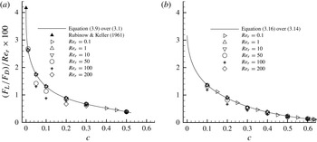
1. Introduction
It is known that a spinning object moving in a viscous fluid experiences a force orthogonal to the plane spanned by the direction of the object’s translational motion and its spin axis. This force accounts for the curved trajectory of spinning balls in sports such as soccer, tennis and golf. This transverse force, now usually termed the Magnus lift force, was first experimentally observed on spinning spheres by Robins in 1742 and then on rotating cylinders by Magnus in 1853 (Barkla & Auchterlonie Reference Barkla and Auchterlonie1971). The explanation for this phenomenon was not given until the introduction of boundary-layer theory by Prandtl in 1904 (see Anderson Reference Anderson2005). Considering the object to be a sphere, the particle Reynolds number (usually referred to as Reynolds number for conciseness) used to characterize the flow dynamics is usually defined as
 $$\begin{eqnarray}\mathit{Re}={\it\rho}\left|\boldsymbol{U}\right|d/{\it\mu}\end{eqnarray}$$
where
 $\boldsymbol{U}$
is the steady-state superficial fluid velocity, defined as the fluid velocity averaged over the total volume of the system,
 $d$
is the diameter of the sphere, and
 ${\it\rho}$
and
 ${\it\mu}$
are the density and the dynamic viscosity of the fluid, respectively. The Reynolds numbers at which the aforementioned phenomena occur are usually very large. This paper will focus on computing the Magnus lift force for small values of the Reynolds number and hence the primary cause of the lift force for large Reynolds numbers, flow separation, is no longer involved in the flow dynamics. In the range of low Reynolds numbers, the Magnus effect is a particular manifestation of Bernoulli’s theorem and the lift force is mainly generated by the pressure differences on opposite sides of the spinning object.
Rubinow & Keller (Reference Rubinow and Keller1961) theoretically calculated the lift force caused by particle rotation at low Reynolds numbers. The lift force can be expressed as
 $$\begin{eqnarray}\boldsymbol{F}_{\!L}=-{\rm\pi}d^{3}{\it\rho}{\bf\omega}\times \boldsymbol{U}/8,\end{eqnarray}$$
where
 ${\bf\omega}$
is the angular velocity of the sphere. Dividing the lift force by the Stokes drag
 $$\begin{eqnarray}\boldsymbol{F}_{\!DS}=3{\rm\pi}d{\it\mu}\boldsymbol{U},\end{eqnarray}$$
we have the magnitude of the normalized lift force as follows:
 $$\begin{eqnarray}F_{L}=\mathit{Re}_{r}\sin ({\it\theta})/24,\end{eqnarray}$$
where
 $$\begin{eqnarray}\mathit{Re}_{r}={\it\rho}|{\bf\omega}|d^{2}/{\it\mu}\end{eqnarray}$$
is termed the rotational Reynolds number for characterizing the rotational movement of spheres, and
 ${\it\theta}$
is the angle between vectors
 ${\bf\omega}$
and
 $\boldsymbol{U}$
. It can be seen in (1.4) that the lift force is in direct proportion to
 $\mathit{Re}_{r}$
at small Reynolds numbers.
Later, Saffman (Reference Saffman1965) obtained an analytical solution of the lift force acting on a rotating sphere in a linear unbounded shear flow by using matched asymptotic expansions. His expression for the lift force can be given by (Kurose & Komori Reference Kurose and Komori1999)
 $$\begin{eqnarray}F_{L}=6.46{\it\nu}{\it\rho}a^{2}U_{c}(\left|{\it\alpha}_{s}\right|/{\it\nu})^{1/2}-11{\it\rho}U_{c}{\it\alpha}_{s}a^{3}/8+{\rm\pi}{\it\rho}U_{c}{\it\omega}a^{3},\end{eqnarray}$$
where
 $U_{c}$
is the fluid velocity on the streamline through the centre of the sphere,
 $a$
is the radius of the sphere,
 ${\it\alpha}_{s}$
is the fluid shear rate of the mean flow, and
 ${\it\nu}$
is the kinematic viscosity of the fluid. The first two terms on the right-hand side are due to the fluid shear, while the third term represents the Magnus lift force. Saffman commented that unless the rotation speed is significantly greater than the shear rate, and for a freely rotating particle
 ${\it\omega}={\it\alpha}_{s}/2$
, the lift force due to particle rotation is an order of magnitude lower than that due to the shear when the Reynolds number is small. Recently, through direct numerical simulations (DNS), Bagchi & Balachandar (Reference Bagchi and Balachandar2002) found that, even in finite-Reynolds-number regimes, the lift due to free particle rotation (induced by flow shear) is less significant than shear-induced lift on the particle.
The coupling between the Reynolds number
 $\mathit{Re}$
and the dimensionless shear rate
 ${\it\alpha}_{s}^{\ast }~({\it\alpha}_{s}^{\ast }={\it\alpha}_{s}a/U_{c})$
was numerically investigated by Dandy & Dwyer (Reference Dandy and Dwyer1990). The results show that the ratio between the lift force and the drag force is less than 0.07 over all simulated
 $\mathit{Re}~(0.1\leqslant \mathit{Re}\leqslant 100)$
when a relatively large
 ${\it\alpha}_{s}^{\ast }$
is used (
 ${\it\alpha}_{s}^{\ast }=0.1$
). Therefore, only the drag force and particle gravity are considered to be responsible for the dynamics of fluid–particle flows in simulations of many industrially important reactor systems (Zou, Guo & Chan Reference Zou, Guo and Chan2008; Xu et al.
Reference Xu, Chen, Liu, Ge and Li2012). The Magnus lift force, believed to be even less important than the lift force due to flow shear (the Saffman force), is usually neglected.
Though the free particle rotation only causes very insignificant Magnus lift force, this may not be how the particles behave in realistic gas–solids systems. Many investigators (e.g. Bagnold Reference Bagnold1973; White & Schulz Reference White and Schulz1977) have shown the importance of lifting forces in saltation trajectories of sand grains. Through high-speed motion pictures (
 $2000~\text{f.p.s.}$
), White & Schulz (Reference White and Schulz1977) reported that the saltating spherical glass microbeads were spinning at a rate of several hundred revolutions per second. They pointed out that the high spinning rates are generally obtained by collisions with the sand surface. They also found that including the Magnus lift force can increase the height of sand motion by 50 %, resulting in remarkable agreement between numerical trajectory solutions and the filmed trajectories. These observations and calculations were confirmed by another set of experiments performed by White (Reference White1982). Many developments have been made based on White & Schulz’s work (e.g. Zou et al.
Reference Zou, Cheng, Zhang and Zhao2007; Kang & Zou Reference Kang and Zou2011). It is worth mentioning that Zou et al. (Reference Zou, Cheng, Zhang and Zhao2007) reported that in terms of the height and the horizontal distance increases, the Magnus force contributes several times more than the Saffman force does.
With the use of high-speed imaging cameras, investigators found that the majority of particles are rotating at high speeds in circulating fluidized bed (CFB) risers (Wu et al.
Reference Wu, Wang, Luo, Fang and Cen2008; Shaffer, Shadle & Breault Reference Shaffer, Shadle and Breault2009). Experiments show that the high rotating rates are caused by strong frictional collisions, including both inter-particle collisions and particle–wall collisions. Wu et al. (Reference Wu, Wang, Luo, Fang and Cen2008) reported that the mean and maximum rotating rates of particles with a diameter of 0.5 mm were around
 $300~\text{rev}~\text{s}^{-1}$
and
 $2000~\text{rev}~\text{s}^{-1}$
, respectively. Considering that the kinematic viscosity of air is around
 $1.5\times 10^{-5}~\text{m}^{2}~\text{s}^{-1}$
, the rotational Reynolds numbers corresponding to these rotating rates are 30 and 210 respectively. The data from Shaffer et al. (Reference Shaffer, Shadle and Breault2009) yield even larger values of rotational Reynolds number, which are around 90 and 350, respectively. It needs to be mentioned that the rotational Reynolds number due to free particle rotation is usually much less than unity. It is also helpful to use the dimensionless angular speed
 ${\it\Gamma}~({\it\Gamma}={\it\omega}a/U_{c})$
to characterize the relative importance of the rotational movement (e.g. Tsuji, Morikawa & Mizuno Reference Tsuji, Morikawa and Mizuno1985; Kurose & Komori Reference Kurose and Komori1999). Here, an equivalent definition of
 ${\it\Gamma}$
would be
 ${\it\Gamma}=0.5\,\mathit{Re}_{r}/\mathit{Re}$
when the angular velocity is perpendicular to the mean flow. In typical CFB risers, while
 $\mathit{Re}_{r}$
has a magnitude of
 $O(10^{2})$
, as mentioned above
 $\mathit{Re}$
is usually between
 $O(10)$
and
 $O(10^{2})$
. This makes
 ${\it\Gamma}$
in the range of
 $O(1)$
and
 $O(10)$
. For individual particles,
 ${\it\Gamma}$
may range from zero to
 $O(10^{3})$
since, at some instant, individual particles can be completely non-rotational or rotating fast with an almost vanishing
 $\mathit{Re}$
. To explore the effects of particle rotation in a wide range of
 ${\it\Gamma}$
, in this work simulations are performed at a small
 $\mathit{Re}$
of around 0.2 with
 $\mathit{Re}_{r}$
changing from practically zero to
 $O(10^{2})$
.
In computational fluid dynamics (CFD), researchers (e.g. Goldschmidt Reference Goldschmidt2001; Sun & Battaglia Reference Sun and Battaglia2006) have realized that the absence of particle rotation and subsequent energy losses is a deficiency of the multi-fluid model, in contrast to the discrete particle model (DPM), which incorporates physics at the particle level, such as collisions and particle rotation, and simulates particle behaviour that is closer to experimentally observed conditions. After formulating a particle rotation model to account for the energy dissipation due to particle rotation, Sun & Battaglia (Reference Sun and Battaglia2006) and Wang et al. (Reference Wang, Hao, Lu, Yang, Xu and Liu2012) found that the bubble dynamics and time-averaged bed behaviour were better captured in gas-fluidized beds using the multi-fluid models. The CFD-DPM, also known as CFD-DEM (CFD-discrete element model), was first proposed by Tsuji et al. (Reference Tsuji, Morikawa, Tanaka, Nakatsukasa and Nakatani1987), Tsuji, Tanaka & Ishida (Reference Tsuji, Tanaka and Ishida1992), Tsuji, Kawaguchi & Tanaka (Reference Tsuji, Kawaguchi and Tanaka1993) and rationalized by Xu & Yu (Reference Xu and Yu1997, Reference Xu and Yu1998). This approach gives realistic pictures of particle motion by applying Newton’s laws of motion to individual particles. The dynamics of continuum fluid is solved using traditional CFD based on the local averaged Navier–Stokes equations. By this approach, many fluid–particle interaction forces with different physical origins, including the Magnus force, can be implemented in a rather straightforward way (Zhu et al.
Reference Zhu, Zhou, Yang and Yu2007). Using the CFD-DPM with a simple particle–wall collision model, Tsuji et al. (Reference Tsuji, Morikawa, Tanaka, Nakatsukasa and Nakatani1987) investigated the motion of particles and fluid in a horizontal channel. They found that some particles were lifted to a higher position by the Magnus force and thus the particles were dispersed widely in the pipe cross-section. By employing a sticking–sliding collision model to solve the particle–particle collisions and the particle–wall collisions, Lun & Liu (Reference Lun and Liu1997) also found that the Magnus force played a significant role in suspending the solid phase in a horizontal channel. They also reported that
 $\mathit{Re}_{r}$
of particles ranged from approximately 120 to 1360 for all the simulated cases, which are much greater than the measurements conducted by Wu et al. (Reference Wu, Wang, Luo, Fang and Cen2008) and Shaffer et al. (Reference Shaffer, Shadle and Breault2009). Schellander, Schneiderbauer & Pirker (Reference Schellander, Schneiderbauer and Pirker2013) developed a new numerical model based on Eulerian–Lagrangian discrete phase approaches and found that the results were significantly improved in terms of the average particle velocity and solid volume fraction. They attributed this improvement to the inclusion of the Magnus force.
To the best of the authors’ knowledge, the solution of Rubinow & Keller (Reference Rubinow and Keller1961) is the only available theory for the Magnus force. Unfortunately, their theory is only valid at the zero-solid-volume-fraction limit in the low-Reynolds-number regime. Some researchers (e.g. White & Schulz Reference White and Schulz1977; Zou et al.
Reference Zou, Cheng, Zhang and Zhao2007; Kang & Zou Reference Kang and Zou2011) directly used Rubinow & Keller’s solution at all conditions, based on the belief that the Magnus force should be around the same order of magnitude, while other researchers (e.g. Barkla & Auchterlonie Reference Barkla and Auchterlonie1971; Tsuji et al.
Reference Tsuji, Morikawa and Mizuno1985; Lun & Liu Reference Lun and Liu1997; Oesterle & Dinh Reference Oesterle and Dinh1998; Loth Reference Loth2008) invested much effort in developing empirical models of the Magnus force based on experimental measurements. Tsuji et al. (Reference Tsuji, Morikawa and Mizuno1985) clearly stated that the Magnus force is proportional to the dimensionless angular speed
 ${\it\Gamma}$
when
 $\mathit{Re}$
is in the range from 550 to 1600, indicating that the Magnus force may become very significant when
 ${\it\Gamma}$
is quite large. Later, Oesterle & Dinh (Reference Oesterle and Dinh1998) reported that the proportionality tends to decrease with increasing
 ${\it\Gamma}$
in the range
 $10<\mathit{Re}<140$
. For reviews on empirical models, the reader can refer to Loth (Reference Loth2008) and Crowe et al. (2012).
Moreover, DNS of a spinning sphere have been performed to calculate the Magnus force in different Reynolds number regimes (e.g. Kurose & Komori Reference Kurose and Komori1999; Zhou & Fan Reference Zhou and Fan2014). Kurose & Komori’s results showed that, at
 $\mathit{Re}=500$
, the Magnus force is around 50 % of the drag force when a sphere spins at a large
 $\mathit{Re}_{r}$
of 250 (note, in their paper, this spinning rate is represented by
 ${\it\Gamma}$
with a value of 0.25). The recent simulations by Zhou & Fan (Reference Zhou and Fan2014) show that, in the low-Reynolds-number flow regime, the Magnus force reaches around 16 % and 65 % of the drag force when a sphere spins at
 $\mathit{Re}_{r}$
of 10 and 50, respectively. It should be mentioned that the above investigations, including experimental measurements and numerical simulations, solely pay attention to the Magnus force at the zero limit of solid volume fractions, even though the Reynolds number regime varies. Nevertheless, these investigations, especially the two DNS studies, have demonstrated that the Magnus force could be significant when particles spin at high speeds. It is therefore very important to conduct more comprehensive computations to evaluate the Magnus force experienced by the rotating particles in particle-laden flows. With regard to the torque acting on rotating spheres, Takagi (Reference Takagi1977) and Dennis, Singh & Ingham (Reference Dennis, Singh and Ingham1980) have analytically obtained the solution for a rotating sphere in a fluid at rest. However, their theories only gave the result of the torque at practically zero solid volume fraction and the Magnus force was not calculated due to the essentially zero Reynolds number of the flow.
The drag force in the low-Reynolds-number regime has been obtained analytically at various solid volume fractions in both ordered arrays of spheres (Hasimoto Reference Hasimoto1959; Sangani & Acrivos Reference Sangani and Acrivos1982; Zick & Homsy Reference Zick and Homsy1982) and random arrays of spheres (Kim & Russel Reference Kim and Russel1985; Ladd Reference Ladd1990). In these analytical studies, particle rotation is not allowed, and hence, the solutions of the Magnus force and the torque are not pursued.
As mentioned above, the problem of flow through rotating particles is important in many processes involving particle transport and fluidization. In spite of its wide importance, solutions of the Magnus lift force due to particle rotation are generally limited to conditions of practically zero solid volume fractions. The aim of this work is to obtain accurate results that quantify the Magnus force at various solid volume fractions from practically zero to the close-packed limit by using surface-resolved DNS since obtaining the solution using analytical approaches is difficult, if not impossible. The simulations are performed in both ordered arrays and random arrays of spheres. As a starting point, the flow simulated in this work is limited to the low-Reynolds-number regime. Simulations of flows beyond this regime can be done in a similar manner and are left for future work.
2. Numerical methods
The most recently developed immersed boundary–lattice Boltzmann method (IB-LBM) with second-order accuracy is adopted in this work. Several versions of the numerical method with different time schemes are provided in Zhou & Fan (Reference Zhou and Fan2014). The version with the fourth-order Runge–Kutta scheme is used in this paper.
The mono-disperse arrays of spheres considered in this work have a solid volume fraction
 $$\begin{eqnarray}c=n(4/3){\rm\pi}(a/L)^{3},\end{eqnarray}$$
where
 $a$
is the sphere radius, and
 $n$
is the number of spheres enclosed in a typically cubic computational domain whose volume is
 $L^{3}$
. For each simulation case,
 $a$
is obtained through (2.1) after the specification of
 $c$
,
 $n$
and
 $L$
. In this work, random arrays and the three most common types of ordered arrays are simulated, which are simple cubic (SC), body-centred cubic (BCC) and face-centred cubic (FCC) arrays. For SC, BCC and FCC arrays of spheres,
 $n$
simply equals 1, 2 and 4, respectively. For random arrays of spheres,
 $n$
should be large enough to avoid periodic artifacts. In this paper,
 $n$
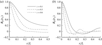
is chosen to be 144. It is important to examine the autocorrelation of the fluid velocity to ensure that the computational domain is sufficient to produce accurate results (Tenneti, Garg & Subramaniam Reference Tenneti, Garg and Subramaniam2011). The streamwise (
 $x$
direction) autocorrelation and the vertical (
 $y$
direction) autocorrelation of the streamwise velocity are depicted in figures 1(a) and 1(b), respectively. It can be seen that all the autocorrelations decay quickly to near zero values except the streamwise autocorrelation for
 $c=0.1$
. This indicates that for small solid volume fractions, more particles and larger computational domains may be required for reduced-period artifacts. However, Tenneti et al. (Reference Tenneti, Garg and Subramaniam2011) have demonstrated that even simulations with 80 particles could produce satisfactory results for
 $c=0.1$
. Therefore, in this work, no attempt has been made to simulate more particles for
 $c=0.1$
. The spanwise (
 $z$
direction) autocorrelation of the streamwise velocity behaves similarly to the vertical one and thus is omitted here.
The autocorrelation functions of the streamwise velocity obtained from the present simulations of steady Stokes flow past a random configuration of spheres at different solid volume fractions. The grid resolution of the simulations is
 $L=192$
;
 $r$
denotes the distance between two points in a specific direction;
 $r_{x}$
and
 $r_{y}$
denote the autocorrelations calculated in the streamwise and vertical directions, respectively. (a) The streamwise autocorrelation of the streamwise velocity,
 $R_{u}(r_{x})$
; (b) the vertical autocorrelation of the streamwise velocity,
 $R_{u}(r_{y})$
.

In order to reduce statistical uncertainty, several random sphere configurations should be simulated for each solid volume fraction. For each configuration, flows in three different directions are simulated to obtain more independent results for ensemble averaging. In this work, the configuration number for each solid volume fraction is usually two or larger, i.e. at least six independent results are obtained for each solid volume fraction of the random-array simulations. Representing the number of independent results by
 $n_{i}$
, the standard deviation of a quantity
 ${\it\phi}$
is calculated from
 ${\rm\Delta}{\it\phi}=\sqrt{\langle ({\it\phi}-\langle {\it\phi}\rangle )^{2}\rangle /(n_{i}-1)}$
, where
 $\langle {\it\phi}\rangle$
is obtained through
 $\langle {\it\phi}\rangle =\sum _{j=1}^{n_{i}}{\it\phi}_{j}/n_{i}$
. In the final average, we intended to omit all values that are outside 2.5 times the standard deviation, as calculated from the initial average. However, no values have been disregarded since all the results are found to be within 2.5 times the standard deviation of the mean. This is attributed to the sophisticated random configuration procedure used in this paper, which is a combination of the standard Monte Carlo procedure (Metropolis et al.
Reference Metropolis, Rosenbluth, Rosenbluth, Teller and Teller1953) and the method of Zinchenko (Reference Zinchenko1994). For details of this procedure, the reader is referred to Hill, Koch & Ladd (Reference Hill, Koch and Ladd2001a
,Reference Hill, Koch and Ladd
b
).
The simulations are initiated with a flow field at rest. A constant pressure gradient
 $\boldsymbol{{\rm\nabla}}p_{e}=\boldsymbol{b}p_{c}{\it\rho}{\it\nu}^{2}/d^{3}$
is imposed to drive the flow through fixed assemblies of spheres, where
 $\boldsymbol{b}$
is a unit vector representing the direction of the pressure gradient and
 $p_{c}$
is used to adjust the magnitude of the constant pressure gradient. In this work,
 $p_{c}$
is chosen such that
 $\mathit{Re}$
of the flow is around or smaller than 0.2. It is found that flows with even smaller
 $\mathit{Re}$
produce indistinguishable forces on spheres, which is consistent with the findings in Van der Hoef, Beetstra & Kuipers (Reference Van der Hoef, Beetstra and Kuipers2005).
To obtain the result for each case, a set of simulations with different grid resolutions is executed. Typically, the grid resolutions used here are
 $L/h=48$
, 72 and 108 for ordered arrays and
 $L/h=108$
, 144 and 192 for random arrays, where
 $L$
and
 $h$
are the size of the computational cube and the lattice spacing, respectively. The retraction distance of
 $r_{d}=0.3h$
is fixed in all the simulations. The final drag force, Magnus lift force and torque for each case are obtained from Richardson extrapolation using the values from the three consecutive meshes (Breugem Reference Breugem2012; Zhou & Fan Reference Zhou and Fan2014). The fluid viscosities adopted in the simulations are computed from
 ${\it\nu}=1.65\text{CFL}/12$
(Zhou & Fan Reference Zhou and Fan2014), where
 $\text{CFL}$
denotes the Courant–Friedrichs–Lewy number. To control the compressibility errors of the LB equation while maintaining the computation stable,
 $\text{CFL}$
is set to 0.8 for solid volume fractions less than 0.3. It is found that compressibility errors grow monotonically with increasing solid volume fraction. Given that compressibility errors can be kept small by either decreasing the fluid viscosity or increasing the ratio of the sphere diameter to the lattice spacing, in this work,
 $\text{CFL}$
is gradually reduced as the solid volume fraction increases to avoid excessively large computational domains. For instance, for random arrays of spheres, the
 $\text{CFL}$
numbers for solid volume fractions
 $c=0.4$
, 0.5, 0.6 and 0.63 are chosen as 0.4, 0.2, 0.15 and 0.1, respectively. To ensure that the compressible errors are negligible, both the maximum magnitude of the divergence of the velocity field
 $\boldsymbol{{\rm\nabla}}\boldsymbol{\cdot }\boldsymbol{u}$
and that of the density fluctuations
 ${\it\delta}{\it\rho}$
are recorded during the simulations. It is found that
 $|\boldsymbol{{\rm\nabla}}\boldsymbol{\cdot }\boldsymbol{u}|_{max}$
and
 $|{\it\delta}{\it\rho}|_{max}$
are usually around
 $1\times 10^{-5}$
and
 $1\times 10^{-4}$
on the finest meshes, respectively, indicating that compressible effects in the simulations can be safely ignored.
2.1. Calculation of the drag force, the Magnus lift force and the torque acting on spheres
The overall force
 $\widetilde{\boldsymbol{F}}$
exerted on a sphere is computed after the flow reaches steady state. In this work, the buoyancy-type force due to the pressure gradient is usually excluded from
 $\widetilde{\boldsymbol{F}}$
. Therefore,
 $\widetilde{\boldsymbol{F}}$
in stage
 $q$
of a time step can be calculated as
 $$\begin{eqnarray}\widetilde{\boldsymbol{F}}^{q}=-\mathop{\sum }_{l}\widetilde{\boldsymbol{F}}_{l}^{q,N_{s}}{\rm\Delta}V_{l}+\frac{\text{d}}{\text{d}t}\left(\int _{V_{p}}{\it\rho}\boldsymbol{u}\text{d}V\right)+V_{p}\boldsymbol{{\rm\nabla}}p_{e},\end{eqnarray}$$
where
 $V_{p}$
is the sphere volume,
 $\boldsymbol{u}$
is the velocity vector of the flow,
 ${\rm\Delta}V_{l}$
is the volume for the
 $l$
th Lagrangian marker,
 $\widetilde{\boldsymbol{F}}_{l}^{q,N_{s}}$
is the force experienced by the
 $l$
th Lagrangian marker, and
 $N_{s}$
represents the total number of force iterations in the multi-direct forcing method. The final value of
 $\widetilde{\boldsymbol{F}}$
is obtained from the following expression:
 $$\begin{eqnarray}\widetilde{\boldsymbol{F}}=\mathop{\sum }_{k=1}^{i}{\it\beta}_{ik}\widetilde{\boldsymbol{F}}^{k},\end{eqnarray}$$
where
 ${\it\beta}_{ik}$
denotes the coefficients of the Runge–Kutta scheme. Here,
 $i=4$
since the four-stage fourth-order Runge–Kutta scheme is used.
It is appropriate to normalize overall force
 $\widetilde{\boldsymbol{F}}$
with the magnitude of the Stokes drag
 $\boldsymbol{F}_{DS}$
. Thus, we have
 $$\begin{eqnarray}\boldsymbol{F}=\widetilde{\boldsymbol{F}}/\left|\boldsymbol{F}_{DS}\right|=\widetilde{\boldsymbol{F}}/3{\rm\pi}d{\it\mu}\left|\boldsymbol{U}\right|,\end{eqnarray}$$
where
 $\boldsymbol{F}$
is used to represent the normalized overall force hereinafter. Also, in the remainder of this paper, all the forces referred to are normalized in the same manner and the word ‘normalized’ is usually omitted for conciseness.
By definition, the drag force
 $\boldsymbol{F}_{D}$
is the force experienced by a sphere in the direction of the flow velocity
 $\boldsymbol{U}$
. Denoting the unit vector in the direction of
 $\boldsymbol{U}$
as
 $$\begin{eqnarray}\boldsymbol{n}_{D}=\boldsymbol{U}/\sqrt{\boldsymbol{U }\boldsymbol{\cdot }\boldsymbol{ U}},\end{eqnarray}$$
the drag force can be calculated from
 $$\begin{eqnarray}\boldsymbol{F}_{D}=F_{D}\boldsymbol{n}_{D}=(\boldsymbol{F}\boldsymbol{\cdot }\boldsymbol{n}_{D})\boldsymbol{n}_{D}.\end{eqnarray}$$
The lift force due to particle rotation will be in the direction of
 $-{\bf\omega}\times \boldsymbol{U}$
. Similarly, the unit vector for
 $-{\bf\omega}\times \boldsymbol{U}$
is defined as
 $$\begin{eqnarray}\boldsymbol{n}_{L}=-{\bf\omega}\times \boldsymbol{U}/\sqrt{({\bf\omega}\times \boldsymbol{ U })\boldsymbol{\cdot }({\bf\omega}\times \boldsymbol{ U })}.\end{eqnarray}$$
Then, the lift force can be calculated from
 $$\begin{eqnarray}\boldsymbol{F}_{L{\it\theta}}=F_{L{\it\theta}}\boldsymbol{n}_{L}=(\boldsymbol{F}\boldsymbol{\cdot }\boldsymbol{n}_{L})\boldsymbol{n}_{L},\end{eqnarray}$$
where
 ${\it\theta}$
is the angle between
 ${\bf\omega}$
and
 $\boldsymbol{U}$
and can be obtained by
 $$\begin{eqnarray}{\it\theta}=\arcsin [\left|{\bf\omega}\times \boldsymbol{U}\right|/(\left|{\bf\omega}\right|\,\left|\boldsymbol{U}\right|)].\end{eqnarray}$$
The lift force
 $\boldsymbol{F}_{L{\it\theta}}$
is denoted as
 $\boldsymbol{F}_{L}$
only when
 ${\bf\omega}$
and
 $\boldsymbol{U}$
are perpendicular to each other, i.e.
 ${\it\theta}={\rm\pi}/2$
. The relation between
 $\boldsymbol{F}_{L{\it\theta}}$
and
 $\boldsymbol{F}_{L}$
can be expressed as
 $$\begin{eqnarray}\boldsymbol{F}_{L{\it\theta}}=\boldsymbol{F}_{L}\sin ({\it\theta}).\end{eqnarray}$$
Theoretically, this relation is valid only when both
 $\mathit{Re}$
and
 $\mathit{Re}_{r}$
are small. However, this work will show that this relation is approximately correct in a wide range of
 $\mathit{Re}_{r}$
when
 $\mathit{Re}$
is small.
In three-dimensional space, the cross-product of two orthogonal unit vectors yields the third unit vector
 $$\begin{eqnarray}\boldsymbol{n}_{R}=\boldsymbol{n}_{D}\times \boldsymbol{n}_{L}.\end{eqnarray}$$
The force along the third unit vector, referred to as the residual force, is calculated from
 $$\begin{eqnarray}\boldsymbol{F}_{R}=F_{R}\boldsymbol{n}_{R}=(\boldsymbol{F}\boldsymbol{\cdot }\boldsymbol{n}_{R})\boldsymbol{n}_{R}.\end{eqnarray}$$
In the low-Reynolds-number regime, the force
 $\boldsymbol{F}_{R}$
vanishes in an ordered-array simulation due to the linearity of the Stokes equations and symmetry considerations. However, in a random-array simulation,
 $\boldsymbol{F}_{R}$
may be non-zero due to the fact that a perfectly isotropic random configuration is difficult to achieve. Generally, an anisotropic configuration may direct the flow away from the direction of the imposed pressure gradient, making
 $\boldsymbol{F}$
deviate from
 $\boldsymbol{U}$
even when particle rotation is not present. This phenomenon has been reported by previous studies (e.g. Kriebitzsch, Van der Hoef & Kuipers Reference Kriebitzsch, Van der Hoef and Kuipers2013; Zhou et al.
Reference Zhou, Xiong, Wang, Wang, Ren and Ge2014). However, the underlying reason behind it has not been elaborated. Essentially, a phenomenon of this kind is quite common in practice. An extreme but simple example of an anisotropic configuration resembles the shape of an aerofoil, which can be formed by stacking a number of spheres in an organized way. When the fluid flows around an aerofoil, it certainly experiences, other than the drag force, a force in a lateral direction, the so-called aerodynamic lift force. The difference is that, in the area of aerodynamics, the generation of the lateral force is not solely due to the anisotropic shape of the aerofoil but also to the boundary layer theory at high Reynolds numbers. Here, we will refer to the force caused by the anisotropy of configurations simply as the ‘configuration force’ and represent it by
 $\boldsymbol{F}_{C}$
. The direction of the configuration force can be quite arbitrary, depending on the specific positioning of the spheres in arrays. For a system without particle rotation,
 $\boldsymbol{F}_{C}$
can be estimated by
 $$\begin{eqnarray}\boldsymbol{F}_{C}=\boldsymbol{F}-\boldsymbol{F}_{D}.\end{eqnarray}$$
For a system with particle rotation, the entire
 $\boldsymbol{F}_{R}$
and part of
 $\boldsymbol{F}_{L}$
come from
 $\boldsymbol{F}_{C}$
. Certainly,
 $\boldsymbol{F}_{C}$
also contributes to
 $\boldsymbol{F}_{D}$
in systems with or without particle rotation. This does not affect the accuracy of
 $\boldsymbol{F}_{D}$
much since
 $\boldsymbol{F}_{C}$
is usually around or less than 1 % of
 $\boldsymbol{F}_{D}$
in magnitude. However,
 $\boldsymbol{F}_{C}$
can be comparable to or even greater than the actual lift force when the rotational Reynolds number is low. This influence on the lift force cannot be appreciably reduced by averaging over limited samples (for details on this issue, see discussions in § 3.2.2). Therefore, to accurately calculate the lift force, a procedure to eliminate the configuration force must be formulated.
Theoretically, in low-Reynolds-number flows, other than the translational movement, the rotational movement of the particles also contributes to the configuration force in anisotropic random arrays. Thus, essentially,
 $\boldsymbol{F}_{C}$
is comprised of
 $\boldsymbol{F}_{C}^{U}$
and
 $\boldsymbol{F}_{C}^{{\it\omega}}$
, which are the average configuration force caused by the translational and rotational movements of the spheres, respectively. To evaluate the magnitude of
 $\boldsymbol{F}_{C}^{{\it\omega}}$
, the direct approach is to simulate systems in which spheres rotate but do not translate, i.e. the systems have a non-zero
 $\mathit{Re}_{r}$
but a literally zero
 $\mathit{Re}$
. However, it is not possible to make
 $\mathit{Re}$
zero without prior knowledge of the force potentially caused by particle rotation. With the linearity of the problem, the configuration force from particle rotation can be easily calculated by conducting simulations with zero pressure gradient. To this end, simulations with
 $\mathit{Re}_{r}=0.1$
are performed at conditions of
 $\boldsymbol{{\rm\nabla}}p_{e}=0$
for various solid volume fractions. It is found that the fluid in steady state still flows in a certain direction with a very small yet non-zero Reynolds number, which is termed
 $\mathit{Re}^{\prime }$
for later use. Since the fluid is flowing with constant velocity, the total force on the fluid should be zero. This yields
 $$\begin{eqnarray}-L^{3}\boldsymbol{{\rm\nabla}}p_{e}-n\boldsymbol{F}_{g\rightarrow s}=0,\end{eqnarray}$$
where
 $\boldsymbol{F}_{g\rightarrow s}$
is the total average force that the fluid exerts on each sphere (including the buoyancy-type force if the pressure gradient is non-zero). From the analysis above, it follows that
 $$\begin{eqnarray}\boldsymbol{F}_{g\rightarrow s}=\boldsymbol{F}_{D}+\boldsymbol{F}_{L}+\boldsymbol{F}_{C}^{U}+\boldsymbol{F}_{C}^{{\it\omega}}-V_{p}\boldsymbol{{\rm\nabla}}p_{e}.\end{eqnarray}$$
It is known that
 $\boldsymbol{F}_{C}^{U}$
is independent of particle rotation and is always minor compared to
 $\boldsymbol{F}_{D}$
. It is also known that for any
 $\mathit{Re}$
, the magnitude of
 $\boldsymbol{F}_{L}$
at
 $\mathit{Re}_{r}=0.1$
is always around
 $10^{-3}$
times of that of
 $\boldsymbol{F}_{D}$
, which is based on the simulation results performed in this work as well as on the theoretical relation (1.4). Keeping these in mind and also considering that
 $\boldsymbol{{\rm\nabla}}p_{e}=0$
, the combination of (2.14) and (2.15) gives
 $$\begin{eqnarray}\boldsymbol{F}_{D}+\boldsymbol{F}_{C}^{{\it\omega}}\approx 0.\end{eqnarray}$$
Therefore, the magnitude of
 $\boldsymbol{F}_{C}^{{\it\omega}}$
can be estimated by that of
 $\boldsymbol{F}_{D}$
, which can be easily determined by
 $\mathit{Re}^{\prime }$
. Through simulations for various solid volume fractions, it is learned that the magnitude of
 $\mathit{Re}^{\prime }$
is generally around
 $O(10^{-6})$
, which is approximately
 $10^{-5}$
times smaller than the Reynolds number used to generate the results in this work, which is around 0.2. This makes the magnitude of
 $\boldsymbol{F}_{C}^{{\it\omega}}$
approximately
 $10^{-5}$
times smaller than that of
 $\boldsymbol{F}_{D}$
obtained at
 $\mathit{Re}\approx 0.2$
due to the linearity of this problem. Also, as just mentioned, the magnitude of
 $\boldsymbol{F}_{L}$
is only around
 $10^{-3}$
times that of
 $\boldsymbol{F}_{D}$
at a small
 $\mathit{Re}_{r}$
of 0.1. All this makes
 $\boldsymbol{F}_{L}$
calculated at
 $\mathit{Re}_{r}=0.1$
and
 $\mathit{Re}\approx 0.2$
approximately
 $10^{2}$
times larger than
 $\boldsymbol{F}_{C}^{{\it\omega}}$
. Moreover, both
 $\boldsymbol{F}_{L}$
and
 $\boldsymbol{F}_{C}^{{\it\omega}}$
are approximately in direct proportion to
 $\mathit{Re}_{r}$
, making
 $\boldsymbol{F}_{C}^{{\it\omega}}$
still negligible compared to
 $\boldsymbol{F}_{L}$
for various
 $\mathit{Re}_{r}$
up to
 $O(10^{2})$
. Therefore, no efforts are made to eliminate
 $\boldsymbol{F}_{C}^{{\it\omega}}$
in this work. These comparisons also indicate that to obtain accurate results for
 $\boldsymbol{F}_{L}$
and
 $\boldsymbol{F}_{D}$
for random arrays,
 $\mathit{Re}_{r}$
and
 $\mathit{Re}$
cannot be chosen arbitrarily small, though, analytically, smaller
 $\mathit{Re}_{r}$
and
 $\mathit{Re}$
yield better linearity of the problem. As far as
 $\boldsymbol{F}_{D}$
is concerned,
 $\mathit{Re}$
may be lowered to around
 $O(10^{-4})$
without significantly affecting the results. However, for better accuracy of
 $\boldsymbol{F}_{L}$
,
 $\mathit{Re}_{r}$
cannot be either too large or too small. A large
 $\mathit{Re}_{r}$
will certainly incur the unwanted nonlinearity. Too small a
 $\mathit{Re}_{r}$
will yield a small
 $\boldsymbol{F}_{L}$
that can be easily contaminated by the configuration force
 $\boldsymbol{F}_{C}^{{\it\omega}}$
. Based on the discussions above, the choice of
 $\mathit{Re}_{r}=0.1$
and
 $\mathit{Re}\approx 0.2$
is used to produce the results in the present work for flows in the Stokes regime.
Other than the drag force and the Magnus lift force, the torque
 $\widetilde{\boldsymbol{T}}$
exerted by the fluid on the rotating sphere is also computed in this work.
 $\widetilde{\boldsymbol{T}}$
in stage
 $q$
of a time step can be calculated as
 $$\begin{eqnarray}\widetilde{\boldsymbol{T}}^{q}=-\mathop{\sum }_{l}\boldsymbol{r}_{l}^{q-1}\times \widetilde{\boldsymbol{F}}_{l}^{q,N_{s}}{\rm\Delta}V_{l}+\frac{\text{d}}{\text{d}t}\left(\int _{V_{p}}\boldsymbol{r}\times ({\it\rho}\boldsymbol{u})\text{d}V\right),\end{eqnarray}$$
where
 $\boldsymbol{r}$
is the position vector relative to the sphere centroid. Similarly to the overall force
 $\widetilde{\boldsymbol{F}}$
, the final value of
 $\widetilde{\boldsymbol{T}}$
is obtained from the following expression:
 $$\begin{eqnarray}\widetilde{\boldsymbol{T}}=\mathop{\sum }_{k=1}^{i}{\it\beta}_{ik}\widetilde{\boldsymbol{T}}^{k}.\end{eqnarray}$$
The torque
 $\widetilde{\boldsymbol{T}}$
due to particle rotation for zero solid volume fraction at low Reynolds numbers has been analytically obtained by Kirchhoff (Reference Kirchhoff1876) and Rubinow & Keller (Reference Rubinow and Keller1961) and given by
 $$\begin{eqnarray}\boldsymbol{T}_{RK}=-{\rm\pi}{\it\mu}d^{3}{\bf\omega}.\end{eqnarray}$$
It is appropriate to normalize the torque
 $\widetilde{\boldsymbol{T}}$
with the magnitude of
 $\boldsymbol{T}_{RK}$
. Hence, the normalized torque
 $\boldsymbol{T}$
can be calculated as
 $$\begin{eqnarray}\boldsymbol{T}=T\boldsymbol{n}_{T}=\widetilde{\boldsymbol{T}}/{\rm\pi}{\it\mu}d^{3}\left|{\bf\omega}\right|,\end{eqnarray}$$
where
 $T$
represents the magnitude of the normalized torque
 $\boldsymbol{T}$
and
 $\boldsymbol{n}_{T}$
is the unit direction vector of
 $\boldsymbol{T}$
. In low-Reynolds-number flows, the present simulations show that the direction of the torque
 $\boldsymbol{T}$
is indistinguishable from the opposite direction of the angular velocity
 ${\bf\omega}$
even when the rotational Reynolds number reaches
 $O(10^{2})$
. Therefore,
 $\boldsymbol{n}_{T}$
can be simply defined by the following expression:
 $$\begin{eqnarray}\boldsymbol{n}_{T}=-{\bf\omega}/\sqrt{{\bf\omega}\boldsymbol{\cdot }{\bf\omega}}.\end{eqnarray}$$
2.2. Procedure to eliminate the configuration force
As mentioned above, the flow is driven by a constant pressure gradient
 $\boldsymbol{{\rm\nabla}}p_{e}$
, whose direction can be prescribed at will. Due to the anisotropy of the generated random arrays, the steady-state flow velocity
 $\boldsymbol{U}$
will not necessarily follow, but instead deviate slightly from, the direction of
 $-\boldsymbol{{\rm\nabla}}p_{e}$
. This means that
 $\boldsymbol{U}$
and hence all the three unit vectors,
 $\boldsymbol{n}_{D}$
,
 $\boldsymbol{n}_{L}$
and
 $\boldsymbol{n}_{R}$
, cannot be determined until steady state of a simulation is obtained. For a simulation with particle rotation in a random array, the force obtained in the direction of
 $\boldsymbol{n}_{L}$
contains both the Magnus lift force and the component of the configuration force in that direction. To calculate and thus eliminate the unwanted configuration force, typically a simulation without particle rotation but with flow in the same direction as the one with particle rotation needs to be performed. Considering that
 $\boldsymbol{U}$
and the three unit vectors may vary as the flow parameters such as
 $\mathit{Re}_{r}$
change, it is very desirable to formulate a procedure that can reproduce the configuration force in arbitrary directions. Thanks to the linearity of Stokes flows, this can be achieved by simulating the flows without particle rotation through the random array in three linearly independent, not necessarily orthogonal, directions. Denoting the three linearly independent directions by
 $\boldsymbol{n}_{DN1}$
,
 $\boldsymbol{n}_{DN2}$
and
 $\boldsymbol{n}_{DN3}$
, an arbitrary direction
 $\boldsymbol{n}_{D}$
in three-dimensional space can be expressed through a linear combination as follows:
 $$\begin{eqnarray}\boldsymbol{n}_{D}={\it\alpha}\boldsymbol{n}_{DN1}+{\it\beta}\boldsymbol{n}_{DN2}+{\it\gamma}\boldsymbol{n}_{DN3}.\end{eqnarray}$$
The coefficients
 ${\it\alpha}$
,
 ${\it\beta}$
and
 ${\it\gamma}$
are solved using the iterative Gauss–Seidel method due to its simplicity and efficiency. Considering the linearity of Stokes flows, the forces exerted on spheres by the fluid flowing in the direction of
 $\boldsymbol{n}_{D}$
can be expressed as
 $$\begin{eqnarray}\boldsymbol{F}_{N}={\it\alpha}\boldsymbol{F}_{N1}+{\it\beta}\boldsymbol{F}_{N2}+{\it\gamma}\boldsymbol{F}_{N3},\end{eqnarray}$$
where
 $\boldsymbol{F}_{N1}$
,
 $\boldsymbol{F}_{N2}$
and
 $\boldsymbol{F}_{N3}$
are the overall force exerted on spheres when the flow is in the direction of
 $\boldsymbol{n}_{DN1}$
,
 $\boldsymbol{n}_{DN2}$
and
 $\boldsymbol{n}_{DN3}$
, respectively. Here, the overall force
 $\boldsymbol{F}_{N}$
is the sum of the drag force and the configuration force. The actual Magnus force
 $\boldsymbol{F}_{L{\it\theta}}$
can then be evaluated by eliminating the contribution from the configuration force in the direction of
 $\boldsymbol{n}_{L}$
, as shown in the expression
 $$\begin{eqnarray}\boldsymbol{F}_{L{\it\theta}}=[(\boldsymbol{F}-\boldsymbol{F}_{N})\boldsymbol{\cdot }\boldsymbol{n}_{L}]\boldsymbol{n}_{L}.\end{eqnarray}$$
Similarly, the influence of particle rotation on residual force can also be evaluated by
 $$\begin{eqnarray}\boldsymbol{F}_{Rr}=[(\boldsymbol{F}-\boldsymbol{F}_{N})\boldsymbol{\cdot }\boldsymbol{n}_{R}]\boldsymbol{n}_{R}.\end{eqnarray}$$
This force essentially is a projection of
 $\boldsymbol{F}_{C}^{{\it\omega}}$
on
 $\boldsymbol{n}_{R}$
by virtue of the analysis in the previous subsection.
To ensure that the unit vectors
 $\boldsymbol{n}_{DN1}$
,
 $\boldsymbol{n}_{DN2}$
and
 $\boldsymbol{n}_{DN3}$
are linearly independent, the pressure gradient used to drive the flow needs to be specified carefully. In this work, the three directions of the pressure gradient for each random array are chosen as follows:
 $$\begin{eqnarray}\boldsymbol{b}_{N1}=(-1,0,0),\quad \boldsymbol{b}_{N2}=(0,-1,0),\quad \boldsymbol{b}_{N3}=(0,0,-1).\end{eqnarray}$$
Naturally, in isotropic arrays, the flow will follow the direction opposite to that of the pressure gradient, resulting in
 $$\begin{eqnarray}\boldsymbol{n}_{DN1}=(1,0,0),\quad \boldsymbol{n}_{DN2}=(0,1,0),\quad \boldsymbol{n}_{DN3}=(0,0,1).\end{eqnarray}$$
However, due to the existence of anisotropy in the computer-generated random arrays, the actual flow directions may slightly deviate from those shown in (2.27). The actual unit vectors can be written as
 $$\begin{eqnarray}\boldsymbol{n}_{DN1}=(n_{11},n_{12},n_{13}),\quad \boldsymbol{n}_{DN2}=(n_{21},n_{22},n_{23}),\quad \boldsymbol{n}_{DN3}=(n_{31},n_{32},n_{33}),\end{eqnarray}$$
in which
 $n_{11}$
,
 $n_{22}$
,
 $n_{33}$
are close to 1 and all other components are near zero, making
 $\boldsymbol{n}_{DN1}$
,
 $\boldsymbol{n}_{DN2}$
and
 $\boldsymbol{n}_{DN3}$
linearly independent. This also ensures that the coefficient matrix of (2.22) is diagonally dominant, guaranteeing that the solution of
 ${\it\alpha}$
,
 ${\it\beta}$
and
 ${\it\gamma}$
can be obtained.
The procedure to eliminate the configuration force from the Magnus lift force may not be exactly valid when
 $\mathit{Re}_{r}$
is in the intermediate range. This is because the linearity property of the flow may have broken down due to the strong disturbance from the fast particle rotation. However, this will not cause a noticeable error in our results since the lift force at relatively large
 $\mathit{Re}_{r}$
has significantly surpassed the configuration force in magnitude. Thus, in the present work, the procedure formulated above is applied to all simulations for random arrays. Moreover, it is found that the effects of the configuration force on the torque are negligible.
For ordered arrays of spheres, no configuration force is involved in the simulations due to the symmetric positioning of spheres. The drag force, Magnus lift force and torque can be obtained directly through (2.6), (2.8) and (2.20). The residual force
 $\boldsymbol{F}_{R}$
used to indicate the magnitude of the configuration force always stays within the machine round-off errors.
3. Results and analysis
3.1. Simulations for ordered arrays of spheres
First, Stokes flows in ordered arrays of spheres are examined without particle rotation. The results for drag forces provide an excellent means of testing the accuracy of the present numerical method over a wide range of solid volume fractions due to the availability of existing theoretical and computational results in the literature. Then, simulations with particle rotation are performed under various conditions.
3.1.1. The drag force
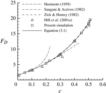
The drag force on spheres in SC arrays is shown in figure 2. It can be seen that the results are in excellent agreement with the theory by Zick & Homsy (Reference Zick and Homsy1982). The differences between the present results and Zick & Homsy’s results are relatively larger at high solid volume fractions, where their analytical computations suffer from limited order approximations. Also shown in the figure are the computational results from Hill et al. (Reference Hill, Koch and Ladd2001a ). Their results scatter around the results of Zick & Homsy, which could be caused by the diameter corrections adopted in their simulations. The analytical results by Hasimoto (Reference Hasimoto1959) and Sangani & Acrivos (Reference Sangani and Acrivos1982) for dilute cases are also provided in figure 2.
The Stokes-flow drag force on non-rotational spheres in SC arrays as a function of the solid volume fraction. The simulation result of Hill et al. (Reference Hill, Koch and Ladd2001a ) and the results from the theories of Hasimoto (Reference Hasimoto1959) and Sangani & Acrivos (Reference Sangani and Acrivos1982) are also shown. The dashed line interpolates the discrete results of Zick & Homsy (Reference Zick and Homsy1982). The solid line represents the fit proposed in this work.

Based on the present simulation results for high solid volume fractions and previous theories for low solid volume fractions, a simple fit for the drag force in the entire packing range is proposed as follows:
 $$\begin{eqnarray}F_{D}=\left\{\begin{array}{@{}l@{}}(1-c)(1-1.7601c^{1/3}+c-1.5593c^{2}+3.9799c^{8/3}-3.0734c^{10/3})^{-1}\quad (c<0.2),\quad \\ 2.812+2.621c+47.99c^{2}+16.99c^{3}\quad (0.2\leqslant c\leqslant {\rm\pi}/6),\quad \end{array}\right.\end{eqnarray}$$
where the equation for
 $c<0.2$
is from Sangani & Acrivos’s theory and
 ${\rm\pi}/6\approx 0.524$
represents the theoretical packing limit of SC arrays of spheres.
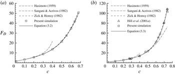
The results for the drag force for BCC and FCC arrays are shown in figure 3, in which it can be seen that the present results agree well with those obtained by Zick & Homsy (Reference Zick and Homsy1982). The expressions
 $$\begin{eqnarray}F_{D}=\left\{\begin{array}{@{}l@{}}(1-c)(1-1.7918c^{1/3}+c-0.3292c^{2})^{-1}\quad (c<0.1),\quad \\ 2.118+6.512c+76.22c^{2}-163.0c^{3}+281.5c^{4}\quad (0.1\leqslant c\leqslant \sqrt{3}{\rm\pi}/8),\quad \end{array}\right.\end{eqnarray}$$
and
 $$\begin{eqnarray}F_{D}=\left\{\begin{array}{@{}l@{}}(1-c)(1-1.7917c^{1/3}+c-0.3020c^{2})^{-1}\quad (c<0.1),\quad \\ \exp (0.6767+5.796c-3.959c^{2}+4.664c^{3})\quad (0.1\leqslant c\leqslant \sqrt{2}{\rm\pi}/6),\quad \end{array}\right.\end{eqnarray}$$
are proposed to fit the present numerical results for BCC and FCC arrays, respectively, in which,
 $\sqrt{3}{\rm\pi}/8$
and
 $\sqrt{2}{\rm\pi}/6$
represent the theoretical packing limit of BCC and FCC arrays, respectively. The theories of Hasimoto (Reference Hasimoto1959) are used in both expressions for higher accuracy in the low range of solid volume fractions (
 $c<0.1$
).
As figure 2, but for (a) BCC and (b) FCC arrays.

3.1.2. The Magnus lift force and the torque due to particle rotation
To calculate the Magnus lift force
 $F_{L}$
, the spheres in arrays are allowed to rotate at various fixed rates from the low to the intermediate range. For each selected solid volume fraction, usually six values of
 $\mathit{Re}_{r}$
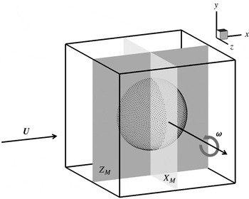
are simulated. Specifically, they are 0.1, 1, 10, 50, 100 and 200. The rotation axis of the spheres is first set perpendicular to the direction of the added pressure gradient, as shown in figure 4. The non-perpendicular case is examined afterwards.
Schematic illustration of flow through SC arrays of rotating spheres. A sphere is positioned in the middle of the computational domain and periodic conditions are implemented in three directions. The angular velocity of the sphere
 ${\bf\omega}$
is in the positive
 $z$
direction. The flow velocity
 $\boldsymbol{U}$
driven by the added pressure gradient is in the positive
 $x$
direction when particle rotation is absent. Two two-dimensional planes
 $X_{M}$
and
 $Z_{M}$
through the centre of the sphere, normal to the
 $x$
and
 $z$
axes, respectively, are also shown.

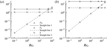
Figure 5 shows the drag force, Magnus lift force and torque acting on the sphere in SC arrays as a function of
 $\mathit{Re}_{r}$
. It can be seen that in general, in the range of
 $\mathit{Re}_{r}$
from practically zero up to
 $O(10^{2})$
, the Magnus lift force linearly increases with
 $\mathit{Re}_{r}$
, whereas the drag force and the torque barely change as
 $\mathit{Re}_{r}$
increases. This indicates that in low-Reynolds-number flows, the nonlinearity caused by the intermediate
 $\mathit{Re}_{r}$
is insignificant. Based on the present results shown in figure 5, the linear dependence of the lift forces on
 $\mathit{Re}_{r}$
can be represented by the following expression:
 $$\begin{eqnarray}F_{L}(\mathit{Re}_{r})=F_{L}|_{Re_{r}=0.1}\mathit{Re}_{r}/0.1,\end{eqnarray}$$
where
 $F_{L}|_{Re_{r}=0.1}$
is the Magnus lift force at
 $\mathit{Re}_{r}=0.1$
. The torque can be expressed as
 $$\begin{eqnarray}T(\mathit{Re}_{r})=T|_{Re_{r}=0.1},\end{eqnarray}$$
and the drag forces can be simply denoted by
 $$\begin{eqnarray}F_{D}(\mathit{Re}_{r})=F_{D}|_{Re_{r}=0},\end{eqnarray}$$
where
 $F_{D}|_{Re_{r}=0}$
is the drag force when particle rotation is absent. Close observation reveals that in high
 $\mathit{Re}_{r}$
ranges for all solid volume fractions, the Magnus lift forces are slightly lower than the linear prediction made by (3.4) (denoted by ‘Straight line 2’ in figure 5). This indicates that the nonlinearity due to high
 $\mathit{Re}_{r}$
is beginning to set in. For high solid volume fractions,
 $F_{L}$
and
 $F_{D}$
start to deviate from the linear predictions of (3.4) and (3.6) at relatively larger
 $\mathit{Re}_{r}$
.
 $T$
is the most insensitive quantity to the increase of
 $\mathit{Re}_{r}$
. For
 $c=0.5$
, the deviations at
 $\mathit{Re}_{r}=200$
from (3.5) are only around 2 %. Generally, in the range of
 $\mathit{Re}_{r}>200$
, the dependence of
 $F_{L}$
,
 $F_{D}$
and
 $T$
on
 $\mathit{Re}_{r}$
tends to be more complicated, and is not pursued in the present paper. Overall, the present results show that the lift force can be very significant in view of the magnitude of the drag force when the sphere rotates at high rates. The figure shows that, for the case of
 $c=0.05$
,
 $F_{L}$
is around 32 % larger than
 $F_{D}$
at
 $\mathit{Re}_{r}=100$
. For
 $c=0.5$
,
 $F_{L}$
is around 39 % and 76 % of
 $F_{D}$
at
 $\mathit{Re}_{r}=100$
and
 $\mathit{Re}_{r}=200$
, respectively. Considering that the maximum
 $\mathit{Re}_{r}$
measured by Wu et al. (Reference Wu, Wang, Luo, Fang and Cen2008) and Shaffer et al. (Reference Shaffer, Shadle and Breault2009) is around two to three hundred, the values of
 $\mathit{Re}_{r}$
simulated here are all within the practical gas–solid flow systems.
The drag force, Magnus lift force and torque as a function of
 $\mathit{Re}_{r}$
in low-Reynolds-number flows for SC arrays of spheres. Three straight lines are drawn for reference. ‘Straight line 1’ is a horizontal line with the constant value of the drag force when particle rotation is absent. ‘Straight line 2’ is governed by (3.4). ‘Straight line 3’ is a horizontal line with the constant value of the torque at
 $\mathit{Re}_{r}=0.1$
. The solid volume fractions for (a) and (b) are 0.05 and 0.5, respectively.

To explore specifically why, at high
 $\mathit{Re}_{r}$
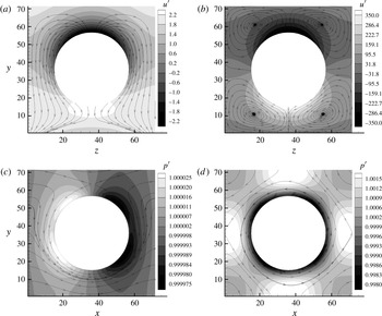
, the Magnus lift force deviates from the linear relation shown in (3.4), both the contours of steady-state normalized streamwise velocity
 $u^{\prime }=u/|\boldsymbol{U}|$
and the streamlines on the middle plane
 $X_{M}$
(see figure 4) are shown in figure 6. Figures 6(a) and 6(b) are the results for
 $\mathit{Re}_{r}=1$
and
 $\mathit{Re}_{r}=100$
, respectively. It can be seen that for both
 $\mathit{Re}_{r}$
,
 $u^{\prime }$
attains negative values at the top and positive values at the bottom of the sphere. This is caused by the particle rotation with
 ${\bf\omega}$
directed in the positive
 $z$
direction (see figure 4). For
 $\mathit{Re}_{r}=1$
, the secondary flow on the middle plane transports the fluid from the top to the bottom of the sphere. This flow helps sustain the
 $u^{\prime }$
distribution caused by particle rotation, which produces the Magnus lift force. However, for
 $\mathit{Re}_{r}=100$
, the secondary flow is dominated by four circulating flows that reside at the corners of the computational cube. This flow pattern hinders the transport of the fluid from the top to the bottom and thus to some degree reduces the difference of
 $u^{\prime }$
at the two sides. Eventually, a Magnus lift force lower than expected from the linear relation will be produced. This flow pattern also explains why the torque increases slightly at large
 $\mathit{Re}_{r}$
(see figure 5) since the inefficient transport of the fluid from the top to the bottom certainly increases the resistance of the rotational motion of the sphere.
(a,b) Contours of the steady-state normalized streamwise velocity
 $u^{\prime }=u/|\boldsymbol{U}|$
and streamlines on the two-dimensional plane
 $X_{M}$
denoted in figure 4. (c,d) Contours of the steady-state normalized pressure
 $p^{\prime }=p/({\it\rho}_{0}/3)$
and streamlines on the two-dimensional plane
 $Z_{M}$
denoted in figure 4. The results are generated from the simulations for a solid volume fraction of 0.1 at the grid resolution of
 $L/h=72$
, where
 $L$
and
 $h$
are the size of the computational cube and the lattice spacing, respectively. For (a,c),
 $\mathit{Re}_{r}=1$
while for (b,d),
 $\mathit{Re}_{r}=100$
.

Figure 6(c,d) shows the distribution of the normalized pressure
 $p^{\prime }$
on the two-dimensional plane
 $Z_{M}$
, where the position of plane
 $Z_{M}$
is denoted in figure 4. In LBM, the pressure is computed as
 ${\it\rho}/3$
and hence the normalized pressure is defined as
 $p^{\prime }=p/({\it\rho}_{0}/3)$
, where
 ${\it\rho}_{0}$
is the initial density of the fluid in the simulation. It can be seen that for
 $\mathit{Re}_{r}=1$
, high and low pressure appears upstream and downstream of the sphere separately, while for
 $\mathit{Re}_{r}=100$
, the pressure distribution becomes approximately symmetric around the sphere. The symmetric pressure distribution is essentially caused by the fast rotation motion of the sphere, which promotes an instant communication of the flow information between upstream and downstream (see the streamlines in figure 6(d)). This pressure distribution tends to decrease the overall force experienced by the sphere and thus the Magnus lift force would be lower than the prediction from the linear relation. Moreover, it is noted that the decreasing trend of
 $F_{L}$
with increasing
 $\mathit{Re}_{r}$
has been observed in experiments at intermediate Reynolds numbers performed by Oesterle & Dinh (Reference Oesterle and Dinh1998). However, definitive explanations of this trend were not given because no information on the flow structure can be obtained from their experiments.
Due to the linear dependence of the lift forces on
 $\mathit{Re}_{r}$
, the expression for
 $F_{L}$
for various solid volume fractions can be developed solely based on the results obtained at small
 $\mathit{Re}_{r}$
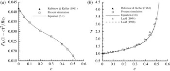
. Figure 7(a) depicts
 $F_{L}$
multiplied by
 $(1-c)^{2}$
divided by
 $\mathit{Re}_{r}$
as a function of
 $c$
. The values are from the computations at
 $\mathit{Re}_{r}=0.1$
, which is small enough to provide accurate proportionalities for higher
 $\mathit{Re}_{r}$
. In order to best fit the present simulation results and also have the correct limiting behaviour for
 $c\rightarrow 0$
, a third-order polynomial is proposed for
 $F_{L}$
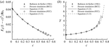
as follows:
 $$\begin{eqnarray}F_{L}(1-c)^{2}/\mathit{Re}_{r}=(-0.287c^{3}+0.228c^{2}-0.0904c+1/24).\end{eqnarray}$$
The largest deviation of this fit from the present numerical results is less than 1 %.
(a) The Magnus lift force
 $F_{L}$
multiplied by the porosity squared divided by the rotational Reynolds number on the rotational spheres in SC arrays as a function of the solid volume fraction. (b) The torque
 $T$
on the rotational spheres in SC arrays as a function of the solid volume fraction: the dashed line is the numerical solution of the Stokes equations (Ladd Reference Ladd1988); the open triangles represent the results obtained using a LBM by Ladd (Reference Ladd1994). Also shown in (a,b) are solid lines representing the best fit to the present results at
 $\mathit{Re}_{r}=0.1$
and the theoretical results calculated by Rubinow & Keller (Reference Rubinow and Keller1961) at zero solid volume fraction.

For the torque, an expression is proposed as follows:
 $$\begin{eqnarray}T=(-14.09c^{4}+10.26c^{3}-2.916c^{2}-0.7480c+1)^{-1}.\end{eqnarray}$$
This fit naturally produces the correct results at the limit of vanishing
 $c$
, which is
 $T=1$
predicted by Rubinow & Keller (Reference Rubinow and Keller1961) as well as Kirchhoff (Reference Kirchhoff1876). The largest deviation of this fit from the present numerical results is less than 1 %. The results for the torque over a wide range of solid volume fractions are also confirmed by the numerical solution of the Stokes equations (Ladd Reference Ladd1988) and the simulation results by Ladd (Reference Ladd1994), which are shown in figure 7(b).
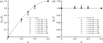
The effect of the angle between the rotation axis of the sphere and the flow direction is also explored in this work. Figure 8 depicts ratios of the Magnus lift force and the torque at several selected angles of
 ${\it\theta}=0$
,
 ${\rm\pi}/6$
,
 ${\rm\pi}/4$
and
 ${\rm\pi}/3$
, to their values at
 ${\it\theta}={\rm\pi}/2$
, respectively. Generally, the torque and the drag force (not shown) stay basically unchanged as
 ${\it\theta}$
varies. The lift force is found to be approximately proportional to
 $\mathit{Re}_{r}\sin ({\it\theta})$
, which is the rotational Reynolds number defined by the component of the angular velocity perpendicular to the flow direction. Thus, for arbitrary rotation axis directions and solid volume fractions, the dependence of the Magnus force on the rotational Reynolds number can be well described by
 $$\begin{eqnarray}F_{L}(\mathit{Re}_{r};{\it\theta};c)=\mathit{Re}_{r}\sin ({\it\theta})(-0.287c^{3}+0.228c^{2}-0.0904c+1/24)/(1-c)^{2}\quad (c\leqslant {\rm\pi}/6).\end{eqnarray}$$
The drag force relation, (3.1), and the torque relation, (3.8), still apply regardless of the values of
 $\mathit{Re}_{r}$
and
 ${\it\theta}$
due to their insensitivity to these rotation-related parameters. It should be mentioned that at high rotational Reynolds numbers, the nonlinearity of the flow starts to set in and produces deviations from (3.8) and (3.9), as one can observe from figures 5 and 8. In the range of smaller rotational Reynolds number,
 $\mathit{Re}_{r}<10$
, (3.1), (3.8) and (3.9) can be used for all the solid volume fractions with less than 1 % error. For larger
 $\mathit{Re}_{r}$
, the errors of these relations generally decrease as the solid volume fraction increases. For low solid volume fractions,
 $c<0.1$
, (3.1), (3.8) and (3.9) can be used in the range of
 $\mathit{Re}_{r}<50$
with errors less than approximately 5 %, 2 % and 15 %, respectively. While for high solid volume fractions,
 $c>0.3$
, with almost the same error thresholds, these relations can be used up to approximately
 $\mathit{Re}_{r}=100$
.
(a) The ratios of the Magnus lift force at several selected angles
 ${\it\theta}=0$
,
 ${\rm\pi}/6$
,
 ${\rm\pi}/4$
and
 ${\rm\pi}/3$
to the Magnus lift force at
 ${\it\theta}={\rm\pi}/2$
; (b) the same as (a), but for the torque.

The results for the Magnus lift force and the torque for BCC and FCC arrays are depicted in figure 9. The proposed expressions for the Magnus lift force for BCC and FCC arrays are
 $$\begin{eqnarray}F_{L}(1-c)^{2}/\mathit{Re}_{r}=(-0.0478c^{3}+0.0853c^{2}-0.0890c+1/24)\quad (c\leqslant \sqrt{3}{\rm\pi}/8)\end{eqnarray}$$
and
 $$\begin{eqnarray}F_{L}(1-c)^{2}/\mathit{Re}_{r}=(-0.0546c^{3}+0.0992c^{2}-0.0930c+1/24)\quad (c\leqslant \sqrt{2}{\rm\pi}/6),\end{eqnarray}$$
respectively. The expressions for the torque for BCC and FCC arrays are
 $$\begin{eqnarray}T=(-2.890c^{4}+2.924c^{3}-1.154c^{2}-0.8444c+1)^{-1}\quad (c\leqslant \sqrt{3}{\rm\pi}/8)\end{eqnarray}$$
and
 $$\begin{eqnarray}T=(-2.280c^{4}+2.568c^{3}-1.093c^{2}-0.8406c+1)^{-1}\quad (c\leqslant \sqrt{2}{\rm\pi}/6),\end{eqnarray}$$
respectively. Similar to SC arrays, more general Magnus lift relations for BCC and FCC arrays accounting for arbitrary rotation axis directions can be obtained.
(a) The Magnus lift force
 $F_{L}$
multiplied by the porosity squared over the rotational Reynolds number on the rotational spheres in BCC and FCC arrays as a function of the solid volume fraction. (b) The torque
 $T$
on the rotational spheres in BCC and FCC arrays as a function of the solid volume fraction. Also shown in (a,b) are the theoretical results calculated by Rubinow & Keller (Reference Rubinow and Keller1961) at zero solid volume fraction.

3.2. Simulations for random arrays of spheres
3.2.1. The drag force
Following the procedure outlined in § 2, simulations without particle rotation are performed to calculate the drag force
 $F_{D}$
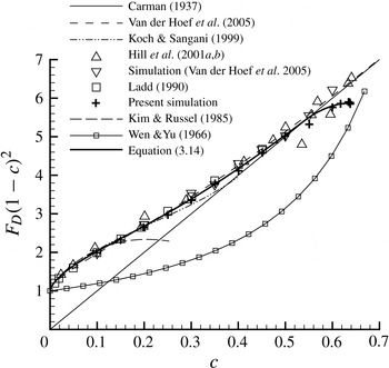
for random arrays of spheres. Figure 10 compares the present results with previous numerical results (Ladd Reference Ladd1990; Hill et al.
Reference Hill, Koch and Ladd2001a
,Reference Hill, Koch and Ladd
b
; Van der Hoef et al.
Reference Van der Hoef, Beetstra and Kuipers2005), theoretical predictions (Carman Reference Carman1937; Kim & Russel Reference Kim and Russel1985; Koch & Sangani Reference Koch and Sangani1999) and an empirical fit based on experimental results (Wen & Yu Reference Wen and Yu1966). The figure shows that the present results agree well with previous numerical values and the Carman relation. The standard errors in
 $F_{D}$
of the present results are typically less than 5 % of the mean (not shown). Based on the present simulation results, the best fit for the drag force in random arrays is proposed as follows:
 $$\begin{eqnarray}F_{D}=\left\{\begin{array}{@{}l@{}}9.9c/(1-c)^{2}+(1-c)^{3}(1+3c^{0.6})\quad (c<0.55),\quad \\ 5.87\sin \left((c/0.637)^{1.75}{\rm\pi}/2\right)/(1-c)^{2}\quad (0.55\leqslant c\leqslant 0.637),\quad \end{array}\right.\end{eqnarray}$$
where 0.637 is the packing limit of a randomly packed bed of mono-disperse spheres in experiments (Scott & Kilgour Reference Scott and Kilgour1969). In the range of
 $c<0.55$
, the present expression takes a similar form to Van der Hoef et al.’s equation. The maximum difference between this expression and the present results is less than 3 %.
The Stokes-flow drag force
 $F_{D}$
(multiplied by the porosity squared) on the non-rotational spheres in random arrays as a function of the solid volume fraction. The simulation results of Ladd (Reference Ladd1990), Hill et al. (Reference Hill, Koch and Ladd2001a
,Reference Hill, Koch and Ladd
b
) and Van der Hoef et al. (Reference Van der Hoef, Beetstra and Kuipers2005) are represented by symbols. The results from the theories of Carman (Reference Carman1937), Kim & Russel (Reference Kim and Russel1985), Koch & Sangani (Reference Koch and Sangani1999) and Van der Hoef et al. (Reference Van der Hoef, Beetstra and Kuipers2005) and the empirical fit of Wen & Yu (Reference Wen and Yu1966) are also shown.

3.2.2. The Magnus lift force and the torque due to particle rotation
For random-array systems, the evaluation of the Magnus lift force can be very complex since, in practical situations, particles may rotate at different speed rates with different rotation axis directions. In this section, a first step is made towards describing the Magnus lift force for practical systems, where all spheres are forced to rotate with the same angular velocity
 ${\bf\omega}$
. Thus, the reported mean Magnus lift force can also be interpreted as an average force experienced by one sphere in various local microstructures due to particle rotation. In the simulations, the rotation axis of the sphere is set to be perpendicular to the direction of the added pressure gradient. However, it may not be perpendicular to the computed superficial flow velocity
 $\boldsymbol{U}$
due to the existence of the configuration force. Since the configuration force is minor relative to the drag force, the angle
 ${\it\theta}$
between
 ${\bf\omega}$
and the steady-state
 $\boldsymbol{U}$
is close to but not necessarily equal to
 ${\rm\pi}/2$
. In this work, it is found that in low-Reynolds-number flows, the relation
 $F_{L{\it\theta}}=F_{L}\sin ({\it\theta})$
(see (2.10)) holds for a wide range of
 $\mathit{Re}_{r}$
not only for ordered arrays but also for random arrays of spheres. Thus, the Magnus lift force at
 ${\it\theta}={\rm\pi}/2$
can be recovered by
 $F_{L}=F_{L{\it\theta}}/\sin ({\it\theta})$
.
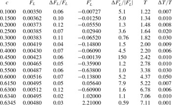
The simulation results of
 $F_{L}$
are given in table 1. The standard deviations in
 $F_{L}$
are also shown in this table, which can be up to approximately 10 % of the mean, especially in the low solid volume fraction range. Also shown in table 1 are the results of the torque
 $T$
and its standard deviation
 ${\rm\Delta}T$
. Typically,
 ${\rm\Delta}T$
is only around 1 % of
 $T$
, indicating that
 $T$
is not as sensitive to different random configurations. The Magnus lift force calculated without the procedure of eliminating the configuration force,
 $F_{L}^{\prime }$
, and its relative standard deviation
 ${\rm\Delta}F_{L}^{\prime }/|F_{L}^{\prime }|$
, are also presented in table 1. It can be seen that
 $F_{L}^{\prime }$
fluctuates in a wide range and
 ${\rm\Delta}F_{L}^{\prime }/|F_{L}^{\prime }|$
attains relatively large values, which indicates that
 $F_{L}^{\prime }$
is not well converged with the limited samples simulated in this work. As pointed out by Tenneti & Subramaniam (Reference Tenneti and Subramaniam2014), even without eliminating the configuration force, ensemble averaging over an adequate number of configurations will yield accurate results. This idea certainly applies to
 $F_{L}$
as well as
 $F_{D}$
and
 $T$
. However, based on the results of
 $F_{L}^{\prime }$
shown in table 1, it can be concluded that to obtain accurate results for
 $F_{L}$
with direct ensemble averaging, many more simulations over different configurations should be performed, which would consume vast computer resources and is not practical.
The Magnus lift force
 $F_{L}$
and torque
 $T$
in random arrays of rotational spheres with
 $\mathit{Re}_{r}=0.1$
at various solid volume fractions
 $c$
.
 $F_{L}^{\prime }$
is the Magnus lift force calculated without eliminating the configuration force.
 ${\rm\Delta}F_{L}$
,
 ${\rm\Delta}F_{L}^{\prime }$
and
 ${\rm\Delta}T$
are the standard deviations in
 $F_{L}$
,
 $F_{L}^{\prime }$
and
 $T$
, respectively.

Similar to ordered arrays, the Magnus lift force increases linearly with increasing
 $\mathit{Re}_{r}$
while the drag force and the torque barely change as
 $\mathit{Re}_{r}$
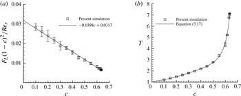
varies. Figure 11(a) depicts the combination
 $F_{L}(1-c)^{2}/\mathit{Re}_{r}$
as a function of the solid volume fraction
 $c$
. The values of
 $F_{L}$
come from the simulations at
 $\mathit{Re}_{r}=0.1$
. Also shown in this figure are the error bars that represent the standard deviations in
 $F_{L}$
. The magnitudes of the error bars are calculated from the results shown in table 1. This figure shows that the dependence of
 $F_{L}(1-c)^{2}/\mathit{Re}_{r}$
on
 $c$
is approximately linear. The best fit to describe this dependence is proposed as follows:
 $$\begin{eqnarray}F_{L}(1-c)^{2}/\mathit{Re}_{r}=-0.0398c+0.0317\quad (c\leqslant 0.637).\end{eqnarray}$$
The maximum difference in the entire range of packing fractions between this relation and the simulation results is only around 5 %, providing good support for the observed linear dependence. It is noted that the Magnus lift force in random arrays is smaller than that in ordered arrays at all solid volume fractions. This is because the random positioning allows some spheres to stay closer to each other and makes spheres hidden behind others experience a smaller flow velocity and consequently, produce less Magnus lift force.
(a) The Magnus lift force
 $F_{L}$
(multiplied by the porosity squared divided by the rotational Reynolds number) on the rotational spheres in random arrays as a function of the solid volume fraction. (b) The torque
 $T$
on the rotational spheres in random arrays as a function of the solid volume fraction. The error bars in (a) and (b) represent the standard deviations in
 $F_{L}$
and
 $T$
, respectively. The results of
 $F_{L}$
and
 $T$
come from the simulations at
 $\mathit{Re}_{r}=0.1$
.

As
 $F_{L{\it\theta}}=F_{L}\sin ({\it\theta})$
yields the Magnus lift force for the case where the angle between the angular velocity
 ${\bf\omega}$
and the steady-state
 $\boldsymbol{U}$
is
 ${\it\theta}$
, a more general Magnus lift relation for arbitrary rotation axis directions and solid volume fractions in random arrays of spheres can be given as
 $$\begin{eqnarray}F_{L}(\mathit{Re}_{r};{\it\theta};c)=\mathit{Re}_{r}\sin ({\it\theta})(-0.0398c+0.0317)/(1-c)^{2}\quad (c\leqslant 0.637).\end{eqnarray}$$
The torque on rotational spheres in random arrays as a function of the solid volume fraction is depicted in figure 11(b). These results also come from the simulations at
 $\mathit{Re}_{r}=0.1$
. It has been illustrated above that
 $T$
remains nearly constant with increasing
 $\mathit{Re}_{r}$
up to
 $O(10^{2})$
and only a slight deviation is observed at large
 $\mathit{Re}_{r}$
. Therefore, the results at a small
 $\mathit{Re}_{r}$
, such as
 $\mathit{Re}_{r}=0.1$
, are sufficient to represent the value of
 $T$
for up to
 $O(10^{2})$
for each solid volume fraction. To best fit the results for all the packing fractions, the following expression is proposed:
 $$\begin{eqnarray}T=(-13.19c^{4}+14.41c^{3}-4.291c^{2}-0.9747c+0.9465)^{-1}\quad (c\leqslant 0.637).\end{eqnarray}$$
The largest deviation of this fit from the present numerical results is less than 1 % for
 $c\leqslant 0.5$
and around 5 % for
 $c>0.5$
. The larger deviation at high
 $c$
is apparently related to the sharp increase of
 $T$
in that range (see figure 11(b)), which essentially is caused by the dramatically shrinking space among spheres as
 $c$
approaches the packing limit. Similar to ordered arrays, the drag relation, (3.14), and the torque relation, (3.17), hold in a wide range of
 $\mathit{Re}_{r}$
regardless of the value of
 ${\it\theta}$
.
3.2.3. Simulations for random arrays of spheres with random angular velocities
In real gas–solid systems, freely moving particles may rotate at different rates with different rotation axis directions. To move a step closer to real-world systems, even in the systems with fixed particles, it is helpful to examine how random angular velocities will affect the results for the systems. In this section, it is assumed that the angular velocities of real systems follow a Gaussian distribution. The assignment of random angular velocities to particles is done as follows. First, all the particles are given the same prescribed mean angular velocity
 ${\bf\omega}$
as done in § 3.2.2. Then, the angular velocity disturbances, which essentially are Gaussian random values with zero mean and a specific standard deviation
 ${\it\sigma}$
, are added to the components in three directions of the angular velocity of all particles. Applying the central limit theorem (Rice Reference Rice1995), the angular velocity disturbances can be generated by repeatedly running Fortran’s random number generator routines. To produce more physically sound results, the standard deviation
 ${\it\sigma}$
of the disturbances is allowed to increase as the magnitude of the mean
 ${\bf\omega}$
increases. Thus, for different
 ${\bf\omega}$
,
 ${\it\sigma}$
is calculated by
 ${\it\sigma}=c_{v}|{\bf\omega}|$
, where
 $c_{v}$
is termed the coefficient of variation. It also needs to be kept in mind that
 $|{\bf\omega}|$
is always determined by (1.5) once
 $\mathit{Re}_{r}$
is prescribed.
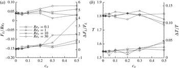
Figure 12 depicts the results for
 $F_{L}/\mathit{Re}_{r}$
and
 $T$
and their relative standard deviations
 ${\rm\Delta}F_{L}/F_{L}$
and
 ${\rm\Delta}T/T$
as a function of
 $c_{v}$
. For each discrete
 $c_{v}$
, four cases with
 $\mathit{Re}_{r}=0.1$
, 1, 10 and 30 are simulated. It can be seen that as
 $c_{v}$
increases, the values of
 $F_{L}/\mathit{Re}_{r}$
and
 $T$
begin to fluctuate around those obtained in the cases of vanishing
 $c_{v}$
, where angular velocity disturbances for particles are absent. This fluctuation of the mean values become more evident when
 $c_{v}$
is larger than 0.1. Due to the relatively stronger nonlinearity associated with larger
 $\mathit{Re}_{r}$
, the magnitude of the fluctuation increases with the increase of
 $\mathit{Re}_{r}$
. For instance, at
 $c_{v}=0.1$
, the maximum deviations of
 $F_{L}/\mathit{Re}_{r}$
and
 $T$
relative to the results at
 $c_{v}=0$
occur at
 $\mathit{Re}_{r}=30$
, which are around 25 % and 1.6 %, respectively. Figure 12 also shows that the relative standard deviations
 ${\rm\Delta}F_{L}/F_{L}$
and
 ${\rm\Delta}T/T$
increase as
 $c_{v}$
increases. It is also noted that the influence of the randomness in the angular velocities on
 $F_{D}$
is not strong and similar to that on
 $T$
. The fluctuation of the mean values and the increase of the relative standard deviations of the results appear to be due to the limited samples (generally six samples) used to generate these results. These phenomena are intrinsically caused by two reasons. One is that the randomness in angular velocities makes the flow possess more microstructures and hence such a system cannot be fully represented with a relatively small number of particles. The other reason is associated with the nonlinearity of the flow brought in by relatively fast-rotating particles, which disturb the local flow strongly and the effects on particles still persist after the average is performed. Moreover, the number of fast-rotating particles increases with increasing
 $c_{v}$
. This adds further complexity to the problem and makes the relative standard deviations even larger.
(a) The Magnus lift force
 $F_{L}/\mathit{Re}_{r}$
on the rotational spheres in random arrays (upper lines) and its relative standard deviation
 ${\rm\Delta}F_{L}/F_{L}$
(lower lines) as a function of the coefficient of variation
 $c_{v}$
. (b) The same as (a), but for the torque
 $T$
and its relative standard deviation
 ${\rm\Delta}T/T$
. The simulations are performed at a solid volume fraction of 0.3.

Simulations in this section are only performed for a solid volume fraction of 0.3. Nevertheless, the results do demonstrate that systems primarily considered in this paper in which particles are all rotating in unison are good approximations of real systems with weak randomness of angular velocities (
 $c_{v}<0.1$
).
3.3. The ratio of the Magnus lift force to the drag force
To clearly identify the importance of the Magnus lift force
 $F_{L}$
relative to the drag force
 $F_{D}$
in both SC arrays and random arrays of spheres, the ratio of
 $F_{L}$
to
 $F_{D}$
is calculated in the entire range of solid volume fractions
 $c$
based on the simulation results as well as the relations proposed in previous subsections. For simplicity, only the values of
 $F_{L}$
at
 ${\it\theta}={\rm\pi}/2$
are used. The results for SC arrays and random arrays of spheres are shown in figures 13(a) and 13(b), respectively. The line in figure 13(a) is calculated by dividing the lift relation, (3.9), by the drag relation, (3.1), while the line in figure 13(b) is calculated by dividing the lift relation, (3.16), by the drag relation, (3.14). For both arrays of spheres, it can be seen that the ratio of
 $F_{L}$
to
 $F_{D}$
first decreases rapidly in the range of
 $c<0.1$
then slows down as
 $c$
further increases. Most of the simulation results agree well with the line calculated from the proposed relations except those at
 $\mathit{Re}_{r}>50$
for low solid volume fractions, which is due, as mentioned above, to the appearance of the nonlinearity of the flow.
Figure 13 shows that the lift force can be very significant and even greater than the drag force when
 $\mathit{Re}_{r}$
is up to
 $O(10^{2})$
, which is still in the practical range as mentioned in the Introduction. Close observation reveals that for both arrays of spheres, when
 $\mathit{Re}_{r}$
reaches 100, the lift-to-drag ratio will be more than unity in the range of
 $c$
of less than approximately 0.17. In the range of high solid volume fractions,
 $c>0.3$
, the lift force can be safely ignored only when
 $\mathit{Re}_{r}$
is less than 10, where the lift-to-drag ratio is generally less than 0.07. However, the lift force can still be significant when spheres are rotating at high rates. For instance, when
 $\mathit{Re}_{r}=100$
, the lift-drag-ratio for
 $c=0.3$
and 0.5 is around 67 % and 39 %, respectively, for SC arrays of spheres, and around 58 % and 23 %, respectively, for random arrays of spheres. The Magnus lift force, appearing in a direction perpendicular to the drag force with a non-negligible magnitude, may appreciably change and complicate the particle fluid dynamics in practical flow systems. Thus, the inclusion of the Magnus lift force is of practical importance in flow simulations. Fortunately, it has been shown that the Magnus lift force can be readily included in the CFD–DPM (Zhu et al.
Reference Zhu, Zhou, Yang and Yu2007). The inclusion of the Magnus lift force in multi-fluid models is somewhat non-trivial due to the fact that rotating speeds of spheres are not tracked in these models. Still, some potential approaches to solving this problem have been proposed in the literature (see Lun Reference Lun1991; Jenkins & Zhang Reference Jenkins and Zhang2002; Sun & Battaglia Reference Sun and Battaglia2006).
The ratio of the Magnus lift force
 $F_{L}$
to the drag force
 $F_{D}$
on the rotational spheres as a function of the solid volume fraction: (a) the results for SC arrays of spheres; (b) the results for random arrays of spheres.

4. Summary
In the present study, steady low-Reynolds-number flows in both ordered arrays and random arrays of non-rotational and rotational spheres are examined over the entire range of packing fractions. The drag forces of the non-rotational spheres in both arrays show good agreement with corresponding existing theories and numerical results. For SC, BCC and FCC arrays of spheres, relations for the drag force equations (3.1)–(3.3), are proposed based on the analytical solutions by Hasimoto (Reference Hasimoto1959) and Sangani & Acrivos (Reference Sangani and Acrivos1982) at low solid volume fractions and the present simulation results at intermediate and high solid volume fractions. These are the first drag force relations that cover the entire solid volume fractions for the three ordered arrays. For random arrays of spheres, based on the present simulation results, a revised relation for the drag force (3.14) is proposed with minor corrections to the one formulated by Van der Hoef et al. (Reference Van der Hoef, Beetstra and Kuipers2005).
To compute the Magnus lift force due to particle rotation, a procedure is formulated to eliminate the influence of the configuration force produced by the anisotropic random arrays of spheres. This procedure applies only for low-Reynolds-number flows where the linearity of the Stokes equations prevails. It is found that the Magnus lift force produced by the rotation movement is approximately in direct proportion to the rotational Reynolds number in the range from practically zero up to
 $O(10^{2})$
, while the drag force and the torque are barely affected by the rotational Reynolds number. Through the evaluation of the ratio between the Magnus lift force and the drag force, it is demonstrated that other than the drag force, the Magnus lift force can be another important factor affecting the overall particle–fluid dynamics. Based on the present simulation results, the Magnus lift force relations, (3.9), (3.10), (3.11) and (3.16), as well as the torque relations, (3.8), (3.12), (3.13) and (3.17), are proposed for the ordered SC, BCC, FCC arrays and random arrays of spheres, respectively. These are the first relations proposed that cover all possible packing fractions. In addition, the effect of the angle between the rotation axis of the sphere and the flow direction is also explored. It is found that the lift force is proportional to the rotational Reynolds number defined by the component of the angular velocity perpendicular to the flow direction. The drag force and the torque are basically unaffected by varying the angle of the rotation axis.
To move a step closer to real-world freely evolving suspensions of mono-disperse spherical particles, the influence of random angular velocities on the results is examined. For random angular velocities with small relative standard deviations (coefficient of variation less than 0.1), the results obtained in systems in which particles are all rotating in unison still persist. For random angular velocities with larger relative standard deviations, the drag force, the Magnus lift force and the torque start to fluctuate and their standard deviations generally increase with the increase of the strength of the randomness in angular velocities. The major reasons for this are discussed in § 3.2.3.
Finally, it should be pointed out that the Magnus lift force has usually been ignored in previous studies of fluid–solid systems. That could be mainly due to unawareness of the fast rotation speeds of particles occurring in practical systems and the lack of Magnus lift force relations for practical random arrays of particles. Recognizing the fast rotation speeds of particles inherently present in the process systems, as experimentally confirmed in the literature and with the relations obtained in this study, the impact of the Magnus lift force on the particle–fluid dynamics in flows can be assessed with ease since the obtained relations can be readily implemented in the CFD–DPM, which is a popular Eulerian–Lagrangian method used for particle–fluid simulations. It should be noted that the present Magnus lift relations can only be used in low-Reynolds-number flows. Calculations of the Magnus lift force in intermediate- and high-Reynolds-number flows are in progress.
Acknowledgements
This work was supported in part by an allocation of computing time from the Ohio Supercomputer Center. The financial support by the US Department of Energy grant no. FE0007520 is gratefully acknowledged. Helpful discussion with Dr K. C. Kwon is appreciated. We would also like to thank Dr A. Z. Zinchenko for his sharing of the code that generates close-packed random sphere configurations used in this work.