2 What is the relation between the local entrainment velocity and the turbulence dissipation?

One might think that the answer to this question is well known and simple and consists of saying that the local entrainment velocity scales as $\unicode[STIX]{x1D708}/\unicode[STIX]{x1D702}_{I}$ as per Corrsin & Kistler (Reference Corrsin and Kistler1955) where the interface thickness $\unicode[STIX]{x1D702}_{I}$ is a length scale, such as for example the Kolmogorov microscale $\unicode[STIX]{x1D702}_{K}\sim (\unicode[STIX]{x1D708}^{3}/\unicode[STIX]{x1D716})^{1/4}$ , which depends on the turbulence dissipation rate $\unicode[STIX]{x1D716}$ . In this section we argue that this answer is too simplistic, if not strictly speaking wrong in general, and we develop a more detailed and complete answer to the question.

It is both rare to find and difficult to obtain fully resolved spatio-temporal three-dimensional (3-D) data of a turbulent flow. It can also be cumbersome and time consuming to store and analyse such data. We therefore develop methods of analysis which can be applied to 2-D planar cuts through the flow, specifically planes orthogonal to the axis of rotational symmetry of an axisymmetric turbulent flow. In this paper we apply our methods to the self-similar axisymmetric turbulent wake.

We start by defining a characteristic local entrainment velocity $v_{n}$ , i.e. characteristic local propagation velocity of the TNT interface, in terms of the time-averaged area $A$ of the fully turbulent region in a plane normal to the axis of symmetry of the flow and the time-averaged length ${\mathcal{L}}$ of the TNT interface in the same plane. This axis of symmetry is aligned with the streamwise direction and coincides with the centreline of the flow. At a streamwise distance $x$ from the wake generator, the rate of change of $A=A(x)$ is given by the integral of the local propagation velocity of the TNT interface over the entire length of the interface. We can express this integral as ${\mathcal{L}}v_{n}$ where the characteristic local entrainment velocity $v_{n}$ is in fact an average local propagation velocity in a sense defined exactly in the appendix A. As the rate of change of $A=A(x)$ can be approximated by $U_{\infty }\,\text{d}A/\text{d}x$ far enough from the wake generator, we write

(2.1) $$\begin{eqnarray}U_{\infty }\frac{\text{d}A}{\text{d}x}={\mathcal{L}}v_{n},\end{eqnarray}$$

where $U_{\infty }$ is the free stream velocity. This equation is derived in the appendix A from first principles, namely incompressibility and the motion of iso-lines.

The instantaneous radial distance $R_{I}$ of the TNT interface from the centreline is a function of streamwise distance $x$ , azimuthal angle $\unicode[STIX]{x1D719}$ around the centreline and time $t$ and is defined in a 2-D plane normal to the centreline. At a distance $x$ from the wake generator, where the turbulent wake is statistically axisymmetric around the centreline, the probability density function (PDF) of $R_{I}$ is independent of $\unicode[STIX]{x1D719}$ and only a function of $x$ . To determine this PDF $P(R_{I};x)$ one can collect statistics over time and $\unicode[STIX]{x1D719}$ in a 2-D plane and test whether this PDF scales with the wake width $\unicode[STIX]{x1D6FF}(x)$ , as first suggested by the intermittency results of Corrsin & Kistler (Reference Corrsin and Kistler1955) and as one might expect in the self-similar region of the turbulence wake, i.e. whether $P(R_{I};x)=\unicode[STIX]{x1D6FF}^{-1}p(R_{I}/\unicode[STIX]{x1D6FF})$ . Such a PDF of $R_{I}$ would suggest that $A(x)\sim \unicode[STIX]{x1D6FF}^{2}(x)$ allowing us to determine the scalings of $v_{n}$ from

(2.2) $$\begin{eqnarray}U_{\infty }\unicode[STIX]{x1D6FF}\frac{\text{d}\unicode[STIX]{x1D6FF}}{\text{d}x}\sim {\mathcal{L}}v_{n}.\end{eqnarray}$$

(The word ‘suggest’ can be replaced by the word ‘imply’ if the interface has only one intersection with nearly every single radial line at nearly every single time in the 2-D plane normal to the $x$ -axis. In such a case, $A(x)$ is the time average of $(\int _{0}^{2\unicode[STIX]{x03C0}}R_{I}^{2}(\unicode[STIX]{x1D719},x,t)\,\text{d}\unicode[STIX]{x1D719})/2$ where $R_{I}(\unicode[STIX]{x1D719},x,t)$ describes the TNT interfacial curve in that 2-D plane at $x$ at time $t$ . Given axisymmetry and ergodicity, it is then possible to write $A(x)=\unicode[STIX]{x03C0}\int _{0}^{\infty }R_{I}^{2}P(R_{I},x)\,\text{d}R_{I}$ which directly implies $A(x)\sim \unicode[STIX]{x1D6FF}^{2}(x)$ if $P(R_{I};x)=\unicode[STIX]{x1D6FF}^{-1}p(R_{I}/\unicode[STIX]{x1D6FF})$ .)

Sreenivasan, Ramshankar & Meneveau (Reference Sreenivasan, Ramshankar and Meneveau1989) introduced and demonstrated the idea that the TNT interface is fractal with a well-defined fractal dimension, which in the case of our 2-D planes would be the fractal dimension $D$ of the TNT interfacial line in the plane, $D$ being such that $1\leqslant D<2$ . The length ${\mathcal{L}}$ of the interfacial line in the 2-D plane at $x$ can therefore be estimated in terms of $D$ , $\unicode[STIX]{x1D6FF}(x)$ and a characteristic thickness $\unicode[STIX]{x1D702}_{I}(x)$ of the interface as follows:

(2.3) $$\begin{eqnarray}{\mathcal{L}}\sim \unicode[STIX]{x1D6FF}(\unicode[STIX]{x1D702}_{I}/\unicode[STIX]{x1D6FF})^{1-D}.\end{eqnarray}$$

To close (2.2) and (2.3) so that $v_{n}(x)$ can be obtained from $\unicode[STIX]{x1D6FF}(x)$ we follow Corrsin & Kistler (Reference Corrsin and Kistler1955) and adopt $\unicode[STIX]{x1D702}_{I}\sim \unicode[STIX]{x1D708}/v_{n}$ . This yields

(2.4) $$\begin{eqnarray}v_{n}/U_{\infty }\sim \left(\frac{\unicode[STIX]{x1D6FF}U_{\infty }}{\unicode[STIX]{x1D708}}\right)^{(1-D)/D}\left(\frac{\text{d}\unicode[STIX]{x1D6FF}}{\text{d}x}\right)^{1/D}.\end{eqnarray}$$

The dependence of the wake width $\unicode[STIX]{x1D6FF}$ on streamwise distance $x$ is critically dependent on the scalings of the centreline turbulence dissipation rate $\unicode[STIX]{x1D716}_{0}(x)$ (see Dairay et al. (Reference Dairay, Obligado and Vassilicos2015), Vassilicos (Reference Vassilicos2015) and references therein). Dairay et al. (Reference Dairay, Obligado and Vassilicos2015) showed, for the axisymmetric self-similar turbulent wake, that

(2.5) $$\begin{eqnarray}\unicode[STIX]{x1D6FF}(x)/\unicode[STIX]{x1D703}\sim \left(\frac{x-x_{0}}{\unicode[STIX]{x1D703}}\right)^{\unicode[STIX]{x1D6FD}}\end{eqnarray}$$

and

(2.6) $$\begin{eqnarray}u_{0}(x)/U_{\infty }\sim \left(\frac{x-x_{0}}{\unicode[STIX]{x1D703}}\right)^{\unicode[STIX]{x1D6FC}},\end{eqnarray}$$

where $\unicode[STIX]{x1D703}$ is the momentum thickness, $x_{0}$ is a virtual origin, $u_{0}$ is the centreline velocity deficit; the exponents $\unicode[STIX]{x1D6FD}=-\unicode[STIX]{x1D6FC}/2=(1+m)/(3+m)$ are determined by the scalings of $\unicode[STIX]{x1D716}_{0}$ , i.e.

(2.7) $$\begin{eqnarray}\unicode[STIX]{x1D716}_{0}(x)\sim \left(\frac{U_{\infty }L_{b}}{\sqrt{K_{0}}\unicode[STIX]{x1D6FF}}\right)^{m}K_{0}^{3/2}/\unicode[STIX]{x1D6FF},\end{eqnarray}$$

where $L_{b}$ is the size of the wake generator and $K_{0}$ is the centreline turbulent kinetic energy. The exponent $m=0$ corresponds to the well-known classical scaling of the turbulence dissipation which is consistent with the Kolmogorov equilibrium theory (see Dairay et al. Reference Dairay, Obligado and Vassilicos2015; Vassilicos Reference Vassilicos2015). The exponent $m=1$ corresponds to the non-equilibrium dissipation scalings found in various high Reynolds number turbulent flows (Goto & Vassilicos Reference Goto and Vassilicos2015; Vassilicos Reference Vassilicos2015) and $m=1/2$ is the exponent reported by Dairay et al. (Reference Dairay, Obligado and Vassilicos2015) and Dairay & Vassilicos (Reference Dairay and Vassilicos2016) for the kind of moderate Reynolds number axisymmetric self-similar turbulent wakes which we study in the following section.

The scalings of $v_{n}$ , obtained from (2.4) and (2.5), are given by

(2.8) $$\begin{eqnarray}v_{n}/U_{\infty }\sim \left(\frac{U_{\infty }L_{b}}{\unicode[STIX]{x1D708}}\right)^{(1-D)/D}\left(\frac{x-x_{0}}{\unicode[STIX]{x1D703}}\right)^{-\unicode[STIX]{x1D6FE}_{e}},\end{eqnarray}$$

where $\unicode[STIX]{x1D6FE}_{e}=(\unicode[STIX]{x1D6FD}(D-1))/D+(1-\unicode[STIX]{x1D6FD})/D$ .

We need to compare these scalings with those of the Kolmogorov velocity $u_{\unicode[STIX]{x1D702}}\sim \unicode[STIX]{x1D708}/\unicode[STIX]{x1D702}_{K}\sim (\unicode[STIX]{x1D708}\unicode[STIX]{x1D716}_{0})^{1/4}$ and to do this we need (2.5), (2.7) and the scalings of $K_{0}$ which can be obtained from (2.5), (2.6) and the Townsend–George relation $K_{0}\sim U_{\infty }u_{0}\,\text{d}\unicode[STIX]{x1D6FF}/\text{d}x$ (see Dairay et al. Reference Dairay, Obligado and Vassilicos2015). (This relation can actually not be found in Townsend (Reference Townsend1976) and George (Reference George, George and Arndt1989) but Townsend (Reference Townsend1976) correctly predicted that $K_{0}$ is proportional to the Reynolds shear stress (the Townsend relation) and George (Reference George, George and Arndt1989) was the first to predict that the Reynolds shear stress scales as $U_{\infty }u_{0}\,\text{d}\unicode[STIX]{x1D6FF}/\text{d}x$ (the George relation). These two relations together give $K_{0}\sim U_{\infty }u_{0}\,\text{d}\unicode[STIX]{x1D6FF}/\text{d}x$ which was ironically predicted by neither Townsend (Reference Townsend1976) nor George (Reference George, George and Arndt1989) who had $K_{0}\sim u_{0}^{2}$ .) We obtain

(2.9) $$\begin{eqnarray}u_{\unicode[STIX]{x1D702}}/U_{\infty }\sim \left(\frac{U_{\infty }L_{b}}{\unicode[STIX]{x1D708}}\right)^{-1/4}\left(\frac{x-x_{0}}{\unicode[STIX]{x1D703}}\right)^{-\unicode[STIX]{x1D6FE}_{\unicode[STIX]{x1D702}}},\end{eqnarray}$$

where $\unicode[STIX]{x1D6FE}_{\unicode[STIX]{x1D702}}=(\unicode[STIX]{x1D6FD}(1+m))/4+((3-m)/8)(\unicode[STIX]{x1D6FD}+1)$ .

The dissipation scaling (2.7) implied by the Kolmogorov equilibrium cascade phenomenology (see Dairay et al. Reference Dairay, Obligado and Vassilicos2015; Vassilicos Reference Vassilicos2015; Obligado et al. Reference Obligado, Dairay and Vassilicos2016) corresponds to $m=0$ which implies $\unicode[STIX]{x1D6FD}=1/3$ and therefore $\unicode[STIX]{x1D6FE}_{\unicode[STIX]{x1D702}}=7/12$ and $\unicode[STIX]{x1D6FE}_{e}=(1+D)/3D$ . There is one and only one value of $D$ for which $\unicode[STIX]{x1D6FE}_{\unicode[STIX]{x1D702}}=\unicode[STIX]{x1D6FE}_{e}$ and therefore $v_{n}/u_{\unicode[STIX]{x1D702}}$ is independent of $x$ and this is $D=4/3$ . This value of $D$ is also the one for which $v_{n}$ and $u_{\unicode[STIX]{x1D702}}$ have the same dependence on global Reynolds number $U_{\infty }L_{b}/\unicode[STIX]{x1D708}$ . Interestingly, this value of $D$ corresponds to the fractal dimension observed experimentally by Sreenivasan et al. (Reference Sreenivasan, Ramshankar and Meneveau1989) and most recently by Mistry et al. (Reference Mistry, Philip, Dawson and Marusic2016) in the far axisymmetric jet (see also references in Mistry et al. (Reference Mistry, Philip, Dawson and Marusic2016) to other papers where such fractal dimension values are found). This value $4/3$ of $D$ is a direct consequence of the Kolmogorov length scale’s $\unicode[STIX]{x1D708}^{3/4}$ dependence on $\unicode[STIX]{x1D708}$ as it also is in the arguments given for it by Sreenivasan et al. (Reference Sreenivasan, Ramshankar and Meneveau1989).

In conclusion, if $m=0$ and $D=4/3$ , then $v_{n}\sim u_{\unicode[STIX]{x1D702}}$ and $\unicode[STIX]{x1D702}_{I}=\unicode[STIX]{x1D708}/u_{e}\sim \unicode[STIX]{x1D702}_{K}$ in the sense that $v_{n}$ and $u_{\unicode[STIX]{x1D702}}$ on the one hand and $\unicode[STIX]{x1D702}_{I}$ and $\unicode[STIX]{x1D702}_{K}$ on the other have the same dependencies on $U_{\infty }L_{b}/\unicode[STIX]{x1D708}$ and $x$ and therefore scale together. This is the case classically envisaged.

However, there are flow regions in various flows where the turbulence dissipation scaling is not the one implied by the Kolmogorov equilibrium cascade but has a new non-equilibrium form (see Dairay et al. Reference Dairay, Obligado and Vassilicos2015; Goto & Vassilicos Reference Goto and Vassilicos2015; Vassilicos Reference Vassilicos2015; Obligado et al. Reference Obligado, Dairay and Vassilicos2016). Such a flow region exists for example in high enough global Reynolds number self-similar axisymmetric turbulent wakes in the range of streamwise distances between approximately $10L_{b}$ and $O(100L_{b})$ where the turbulence dissipation scales as (2.7) with $m=1$ (Dairay et al. Reference Dairay, Obligado and Vassilicos2015; Dairay & Vassilicos Reference Dairay and Vassilicos2016; Obligado et al. Reference Obligado, Dairay and Vassilicos2016). (The $m=0$ scaling appears further downstream (Redford, Castro & Coleman Reference Redford, Castro and Coleman2012) and for reasons different from the Kolmogorov equilibrium cascade, see Goto & Vassilicos (Reference Goto and Vassilicos2016).) The value $m=1$ implies $\unicode[STIX]{x1D6FD}=1/2$ and therefore $\unicode[STIX]{x1D6FE}_{\unicode[STIX]{x1D702}}=5/8$ and $\unicode[STIX]{x1D6FE}_{e}=1/2$ for any value of $D$ . In this case

(2.10) $$\begin{eqnarray}v_{n}/u_{\unicode[STIX]{x1D702}}\sim \left(\frac{U_{\infty }L_{b}}{\unicode[STIX]{x1D708}}\right)^{(1-D)/D+1/4}\left(\frac{x-x_{0}}{\unicode[STIX]{x1D703}}\right)^{1/8}\end{eqnarray}$$

demonstrating clearly that the local entrainment velocity is fundamentally different from $u_{\unicode[STIX]{x1D702}}$ . As in the previous case, though, $v_{n}$ and $u_{\unicode[STIX]{x1D702}}$ have the same Reynolds number dependence if $D=4/3$ but not otherwise.

Interestingly, if one defines a Taylor length scale velocity $u_{\unicode[STIX]{x1D706}}=\unicode[STIX]{x1D708}/\unicode[STIX]{x1D706}$ instead of $u_{\unicode[STIX]{x1D702}}=\unicode[STIX]{x1D708}/\unicode[STIX]{x1D702}_{K}$ , and if one takes $\unicode[STIX]{x1D706}$ to scale according to $\unicode[STIX]{x1D716}_{0}\sim \unicode[STIX]{x1D708}K_{0}/\unicode[STIX]{x1D706}^{2}$ then (2.5), (2.7) and $m=1$ yield $u_{\unicode[STIX]{x1D706}}\sim ((U_{\infty }L_{b})/\unicode[STIX]{x1D708})^{-1/2}(L_{b}/\unicode[STIX]{x1D703})((x-x_{0})/\unicode[STIX]{x1D703})^{-1/2}$ which has the exact same dependence on $x$ as $v_{n}$ . The ratio $v_{n}/u_{\unicode[STIX]{x1D706}}$ is independent of $x$ and depends on Reynolds number according to

(2.11) $$\begin{eqnarray}v_{n}/u_{\unicode[STIX]{x1D706}}\sim \left(\frac{U_{\infty }L_{b}}{\unicode[STIX]{x1D708}}\right)^{(1-D)/D+1/2}.\end{eqnarray}$$

The implication for the characteristic thickness is $\unicode[STIX]{x1D702}_{I}=\unicode[STIX]{x1D708}/v_{n}\sim \unicode[STIX]{x1D706}((U_{\infty }L_{b})/\unicode[STIX]{x1D708})^{-((1-D)/D+1/2)}$ where $\unicode[STIX]{x1D706}\sim ((U_{\infty }L_{b})/\unicode[STIX]{x1D708})^{-1/2}\unicode[STIX]{x1D6FF}$ . The thickness $\unicode[STIX]{x1D702}_{I}$ is therefore effectively $\unicode[STIX]{x1D706}$ in the high Reynolds number non-equilibrium case $m=1$ only if $D=2$ . Otherwise, $\unicode[STIX]{x1D702}_{I}$ and $\unicode[STIX]{x1D706}$ have the same dependence on $x$ but different dependencies on Reynolds number $(U_{\infty }L_{b})/\unicode[STIX]{x1D708}$ , in fact $\unicode[STIX]{x1D702}_{I}/\unicode[STIX]{x1D706}$ is an increasing function of $(U_{\infty }L_{b})/\unicode[STIX]{x1D708}$ but $\unicode[STIX]{x1D702}_{I}/\unicode[STIX]{x1D6FF}\sim ((U_{\infty }L_{b})/\unicode[STIX]{x1D708})^{(1-D)/D}$ is a decreasing function of $(U_{\infty }L_{b})/\unicode[STIX]{x1D708}$ .

The conclusion is that, when $m=1$ , the characteristic thickness $\unicode[STIX]{x1D702}_{I}$ sits between $\unicode[STIX]{x1D706}$ and $\unicode[STIX]{x1D6FF}$ and grows with $x$ in the same way as $\unicode[STIX]{x1D706}$ .

3 DNS of an axisymmetric turbulent wake

In this section we test the assumptions made and results obtained in the previous section with a DNS of a spatially developing axisymmetric turbulent wake generated by a bluff plate placed normal to the incoming laminar free stream. The length $L_{b}$ is the square root of the area of the plate. In such wakes, the turbulence is clearly axisymmetric for $x/L_{b}\geqslant 5$ and the profiles of the mean flow, turbulent kinetic energy, turbulence dissipation and Reynolds shear stress are self-similar for $x/L_{b}$ larger than 10 or 20 (see Dairay et al. Reference Dairay, Obligado and Vassilicos2015; Dairay & Vassilicos Reference Dairay and Vassilicos2016). The relations (2.5), (2.6) and (2.7) are therefore valid for $x/L_{b}\geqslant 10$ and, more specifically, the turbulence dissipation scaling is given by (2.7) with $m=1$ in the range $x/L_{b}=10$ to $x/L_{b}=O(100)$ provided that the Reynolds number $(U_{\infty }L_{b})/\unicode[STIX]{x1D708}$ is large enough, for example $40\,000$ as in the laboratory experiments of Nedić et al. (Reference Nedić, Vassilicos and Ganapathisubramani2013), Dairay et al. (Reference Dairay, Obligado and Vassilicos2015) and Obligado et al. (Reference Obligado, Dairay and Vassilicos2016). At normalised distances $x/L_{b}$ beyond $O(100)$ one expects to find (2.7) with $m=0$ as suggested by the DNS of temporally evolving wakes of Redford et al. (Reference Redford, Castro and Coleman2012).

Unfortunately, current state-of-the-art DNS of spatially developing axisymmetric turbulent wakes cannot reach such high Reynolds numbers and such far downstream distances. The massively parallel such DNS of Dairay et al. (Reference Dairay, Obligado and Vassilicos2015) reached $(U_{\infty }L_{b})/\unicode[STIX]{x1D708}=5000$ and $x/L_{b}=100$ with about $10^{9}$ grid points. The spatial resolution $\unicode[STIX]{x0394}x=\unicode[STIX]{x0394}y=\unicode[STIX]{x0394}z=L_{b}/32$ of the uniform DNS’s Cartesian grid was always below $4\unicode[STIX]{x1D702}_{K}$ between $x/L_{b}=10$ and $x/L_{b}=100$ . The results for $m=0$ and $m=1$ of the previous section are therefore beyond the reach of such DNS. However, in their moderate Reynolds number turbulent wake, Dairay et al. (Reference Dairay, Obligado and Vassilicos2015) reported an intermediate dissipation scaling (2.7) with $m=1/2$ between $x/L_{b}=50$ and $x/L_{b}=100$ . In this work we use the exact same DNS code and same flow configuration and parameters as Dairay et al. (Reference Dairay, Obligado and Vassilicos2015) to test the assumptions made and results obtained in the previous section in the range $50\leqslant x/L_{b}\leqslant 100$ and for $m=1/2$ . Dairay et al. (Reference Dairay, Obligado and Vassilicos2015) validated their simulations of spatially developing axisymmetric turbulent wakes against experimental data.

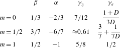
The previous section’s relations (2.5)–(2.9) remain valid for $m=1/2$ but with $\unicode[STIX]{x1D6FD}=3/7$ , $\unicode[STIX]{x1D6FE}_{e}=3/7+1/(7D)$ and $\unicode[STIX]{x1D6FE}_{\unicode[STIX]{x1D702}}\approx 0.61$ (see table 1). In this section we use the DNS to verify our assumptions (i) $P(R_{I};x)=\unicode[STIX]{x1D6FF}^{-1}p(R_{I}/\unicode[STIX]{x1D6FF})$ and $A\sim \unicode[STIX]{x1D6FF}^{2}$ (§ 3.1) and (ii) the fractal nature of the TNT interface with (2.3) and $\unicode[STIX]{x1D702}_{I}\sim \unicode[STIX]{x1D708}/v_{n}$ (§ 3.2); and to test our results (2.8) with $\unicode[STIX]{x1D6FE}_{e}=3/7+1/(7D)$ and (2.9) with $\unicode[STIX]{x1D6FE}_{\unicode[STIX]{x1D702}}\approx 0.61$ (§ 3.3).

Table 1.

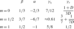
Values of the exponents $\unicode[STIX]{x1D6FD}$ in (2.5),  $\unicode[STIX]{x1D6FC}$ in (2.6),  $\unicode[STIX]{x1D6FE}_{\unicode[STIX]{x1D702}}$ in (2.9) and $\unicode[STIX]{x1D6FE}_{e}$ in (2.8) for different turbulence dissipation scalings (2.7):  $m=0$ in the classical scaling case, $m=1/2$ in the moderate Reynolds number non-equilibrium case and $m=1$ in the high Reynolds number non-equilibrium case. $D$ is the fractal dimension of the TNT interfacial line in the $y$ – $z$ plane; $1\leqslant D<2$ .

A detailed description of the DNS code and flow configuration is given in Dairay et al. (Reference Dairay, Obligado and Vassilicos2015) and references therein and we do not repeat it here for economy of space. The incompressible Navier–Stokes equations are solved with the massively parallel version of the code Incompact3d which is based on sixth-order compact schemes for spatial discretisation on a Cartesian mesh and a third-order Adams–Bashforth scheme for time advancement. An immersed boundary method is used to model the wake-generating bluff plate following the procedure of Parnaudeau et al. (Reference Parnaudeau, Carlier, Heitz and Lamballais2008). The plate is the same as the one used in the DNS and experiments of Dairay et al. (Reference Dairay, Obligado and Vassilicos2015) and Nedić et al. (Reference Nedić, Vassilicos and Ganapathisubramani2013): it has an irregular (fractal-like) periphery which results in higher local Reynolds numbers in the flow for the same global Reynolds number $(U_{\infty }L_{b})/\unicode[STIX]{x1D708}$ . In the present case, the local Taylor length-based Reynolds number $Re_{\unicode[STIX]{x1D706}}$ varies slowly and remains close to 55 throughout the range $50\leqslant x/L_{b}\leqslant 100$ . The DNS of Goto & Vassilicos (Reference Goto and Vassilicos2015) suggest that the non-equilibrium dissipation exponent $m=1$ appears most clearly at values of $Re_{\unicode[STIX]{x1D706}}$ larger that approximately 100 or so. The absence of $m=1$ in the present DNS and those of Dairay et al. (Reference Dairay, Obligado and Vassilicos2015), Dairay & Vassilicos (Reference Dairay and Vassilicos2016) is consistent with this observation.

We adopt inflow/outflow boundary conditions in the streamwise direction with uniform streamwise velocity $U_{\infty }$ without turbulence at the inlet and a 1-D convection equation at the outlet. The streamwise and two lateral directions are all orthogonal to each other and the streamwise size of the computational domain is $L_{x}=120L_{b}$ whereas the lateral sizes are $L_{y}=L_{z}=15L_{b}$ . The plate is located at a distance $10L_{b}$ from the inlet. We collect several variables, including the instantaneous fluid velocity components $u$ in the $x$ direction, $v$ in the $y$ direction and $w$ in the $z$ direction and the modulus $\unicode[STIX]{x1D714}$ of the instantaneous vorticity vector $\unicode[STIX]{x1D735}\times (u,v,w)$ at every grid point of seventeen lateral planes separated by a streamwise distance $5L_{b}$ from $x/L_{b}=20$ to $x/L_{b}=100$ . These planar data are collected every fifth time step in a simulation run of $200\,000$ time steps which corresponds to approximately 109 vortex shedding periods. The initial condition of our simulation is a fully developed instantaneous field obtained and stored by Dairay et al. (Reference Dairay, Obligado and Vassilicos2015).

3.1 DNS results: radial position of interface and area of turbulent region

We define the intersection between the TNT interface and one of our 2-D planar cuts in effectively the same way that various authors have defined the TNT interface in terms of a volume fraction in 3-D space (see da Silva et al. Reference da Silva, Hunt, Eames and Westerweel2014; Watanabe et al. Reference Watanabe, Sakai, Nagata, Ito and Hayase2015, Reference Watanabe, Riley, de Bruyn Kops, Diamessis and Zhou2016). We define the area $A_{t}$ containing all the points in the $y$ – $z$ plane where $\unicode[STIX]{x1D714}$ is larger than a certain threshold $\unicode[STIX]{x1D714}_{th}$ at time $t$ . 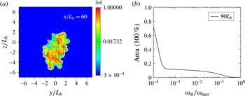Figure 1(a) shows an example of an instantaneous snapshot of the $\unicode[STIX]{x1D714}$ field in the $y$ – $z$ plane at $x/L_{b}=60$ . Similar $\unicode[STIX]{x1D714}$ field snapshots can be obtained at other $x/L_{b}$ locations. The area $A_{t}$ takes different values for different choices of $\unicode[STIX]{x1D714}_{th}$ , but the presence of the TNT interface means that $A_{t}$ will be approximately constant over a significant range of thresholds. Figure 1(b) is a plot of $A$ (normalised by $L_{y}L_{z}$ so as to have an area fraction) defined as the time average of $A_{t}$ conditional on $\unicode[STIX]{x1D714}_{th}(t)/\unicode[STIX]{x1D714}_{max}(t)$ where $\unicode[STIX]{x1D714}_{max}(t)$ is the maximum value of $\unicode[STIX]{x1D714}$ at time $t$ in the plane considered and where $\unicode[STIX]{x1D714}_{th}(t)/\unicode[STIX]{x1D714}_{max}(t)$ is kept constant even though $\unicode[STIX]{x1D714}_{max}(t)$ varies with $t$ . Plots of instantaneous values of $A_{t}/(L_{y}L_{z})$ versus $\unicode[STIX]{x1D714}_{th}/\unicode[STIX]{x1D714}_{max}(t)$ look very similar. A plateau is clearly visible in figure 1(b) between $\unicode[STIX]{x1D714}_{th}/\unicode[STIX]{x1D714}_{max}=4\times 10^{-4}$ and $10^{-2}$ . A similar plateau is also clearly present at all the other streamwise locations where we saved planar data, however over slightly different ranges of $\unicode[STIX]{x1D714}_{th}/\unicode[STIX]{x1D714}_{max}$ for different locations (e.g. between $2\times 10^{-4}$ and $10^{-2}$ at $x/L_{b}=50$ ). (We have repeated the exact same procedure with $\unicode[STIX]{x1D714}_{th}(t)/\unicode[STIX]{x1D714}_{av}(t)$ where $\unicode[STIX]{x1D714}_{av}(t)$ is the instantaneous average of $\unicode[STIX]{x1D714}$ in the $y$ – $z$ plane considered, and with $\unicode[STIX]{x1D714}_{th}/\overline{\unicode[STIX]{x1D714}}(x,0,0)$ where $\overline{\unicode[STIX]{x1D714}}(x,0,0)$ is the time average of $\unicode[STIX]{x1D714}$ at the intersection of the centreline and the $y$ – $z$ plane considered and all our results in this paper remain the same except that the actual values of $\unicode[STIX]{x1D714}_{th}(t)/\unicode[STIX]{x1D714}_{max}(t)$ , $\unicode[STIX]{x1D714}_{th}(t)/\unicode[STIX]{x1D714}_{av}(t)$ and $\unicode[STIX]{x1D714}_{th}/\overline{\unicode[STIX]{x1D714}}(x,0,0)$ are of course different.)

Figure 1.

Definition of interface with examples of the $\unicode[STIX]{x1D714}$ field in a $y$ – $z$ plane (a) and $A/(L_{y}L_{z})$ versus $\unicode[STIX]{x1D714}_{th}/\unicode[STIX]{x1D714}_{max}$ (b). The two plots are given at two different values of $x/L_{b}$ ( $x/L_{b}=60$ on (a) and $x/L_{b}=90$ on (b)) to give a feel for the fact that the interface is well defined at all the values of $x/L_{b}$ considered here. These plots are very similar at all streamwise positions where we saved planar data.

Given the plateau in plots such as figure 1(b), it is possible to define the TNT interface location in a $y$ – $z$ plane with any normalised threshold $\unicode[STIX]{x1D714}_{th}(t)/\unicode[STIX]{x1D714}_{max}(t)$ between $=4\times 10^{-4}$ and $10^{-2}$ . Once such a threshold has been chosen, it is then possible to obtain the radial positions $R_{I}(x,\unicode[STIX]{x1D719},t)$ of the interface from the intersections of the interface with radial straight lines at various azimuthal angles $\unicode[STIX]{x1D719}$ in the $y$ – $z$ plane at $x$ . These radial straight lines start from the centreline’s position $y=z=0$ in this plane. Relatively rarely is there more than one intersection between one of these straight lines and the TNT interface. In such cases the value of $R_{I}$ that we take is the largest one.

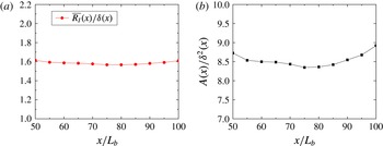
Statistics of $R_{I}$ at a given streamwise location $x/L_{b}$ can be obtained by sampling over $\unicode[STIX]{x1D719}$ and time $t$ . An example is the average interfacial radius $\overline{R_{I}}(x)$ which is a function only of $x$ (averages over $\unicode[STIX]{x1D719}$ and $t$ having been taken). Examples of such average interfacial radii are given in figure 2(a). For this plot, the threshold defining the TNT interface is $\unicode[STIX]{x1D714}_{th}/\unicode[STIX]{x1D714}_{max}=4\times 10^{-4}$ but we have checked that $\overline{R_{I}}(x)$ does not vary significantly if larger values of this normalised threshold are chosen up to approximately $7\times 10^{-3}$ .

Figure 2(a) concentrates attention in the range $x/L_{b}=50{-}100$ where Dairay et al. (Reference Dairay, Obligado and Vassilicos2015) found the $m=1/2$ dissipation scaling and shows that $\overline{R_{I}}(x)\sim \unicode[STIX]{x1D6FF}(x)$ in agreement with original claims by Corrsin & Kistler (Reference Corrsin and Kistler1955). More specifically,

(3.1) $$\begin{eqnarray}\overline{R_{I}}(x)\approx 1.6\unicode[STIX]{x1D6FF}(x)\end{eqnarray}$$

in our case.

The definition of the wake width of an axisymmetric turbulent wake is

(3.2) $$\begin{eqnarray}\unicode[STIX]{x1D6FF}^{2}(x)=\frac{1}{u_{0}}\int _{0}^{\infty }(U_{\infty }-U)r\,\text{d}r,\end{eqnarray}$$

where $U=\overline{u}$ is the mean streamwise velocity averaged over $\unicode[STIX]{x1D719}$ and $t$ and therefore function of $x$ and radius $r$ , and $u_{0}(x)$ equals $U_{\infty }-U(x,r=0)$ where $r=0$ marks the intersection of the plane with the centreline. Following the practical procedure taken in Dairay et al. (Reference Dairay, Obligado and Vassilicos2015) the integral in (3.2) is carried out up to $r=7L_{b}$ , and $U_{\infty }$ in $u_{0}(x)$ and in (3.2) is replaced by $\overline{u}(x,r=7L_{b})$ . This takes care of the finite size of the computational domain and avoids negative values of $U_{\infty }-U$ . The plots in figure 2, where both $\overline{R_{I}}(x)$ and $A$ are normalised by $\unicode[STIX]{x1D6FF}(x)$ , are obtained with this procedure for $\unicode[STIX]{x1D6FF}(x)$ as are all other plots in this paper where $\unicode[STIX]{x1D6FF}(x)$ is required.

Figure 2.

$\overline{R_{I}}(x)/\unicode[STIX]{x1D6FF}(x)$ (a) and $A(x)/\unicode[STIX]{x1D6FF}^{2}(x)$ (b) versus $x/L_{b}$ . These plots were obtained with $\unicode[STIX]{x1D714}_{th}/\unicode[STIX]{x1D714}_{max}=4\times 10^{-4}$ at all $x$ .

Figure 3.

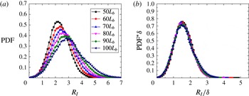
Interfacial radial location PDF: $P(R_{I};x)$ versus $R_{I}$ at different values of $x/L_{b}$ (a) and $\unicode[STIX]{x1D6FF}(x)P(R_{I};x)$ versus $R_{I}/\unicode[STIX]{x1D6FF}(x)$ (b) for different values of $x/L_{b}$ . The normalised threshold $\unicode[STIX]{x1D714}_{th}/\unicode[STIX]{x1D714}_{max}$ used to define the TNT interface at each $x/L_{b}$ varies between $6\times 10^{-4}$ and $10^{-3}$ according to figure 5(a). There is no appreciable difference if these plots are obtained with the same $\unicode[STIX]{x1D714}_{th}/\unicode[STIX]{x1D714}_{max}$ at all $x/L_{b}$ as long as $\unicode[STIX]{x1D714}_{th}/\unicode[STIX]{x1D714}_{max}$ is chosen between $4\times 10^{-4}$ and $7\times 10^{-3}$ (see figure 1).

Figure 2 supports both scalings, $\overline{R_{I}}(x)\approx 1.6\unicode[STIX]{x1D6FF}(x)$ and $A(x)\sim \unicode[STIX]{x1D6FF}^{2}(x)$ , the latter scaling being an important assumption in the theoretical arguments of § 2. The quality of these scalings does not change significantly with normalised threshold $\unicode[STIX]{x1D714}_{th}/\unicode[STIX]{x1D714}_{max}$ . More generally, we find that the PDF $P(R_{I};x)$ takes a self-similar form normalised by $\unicode[STIX]{x1D6FF}(x)$ in the investigated range $50\leqslant x/L_{b}\leqslant 100$ (see figure 3), namely

(3.3) $$\begin{eqnarray}\unicode[STIX]{x1D6FF}(x)P(R_{I};x)=p(R_{I}/\unicode[STIX]{x1D6FF}(x)),\end{eqnarray}$$

where the function $p(R_{I}/\unicode[STIX]{x1D6FF}(x))$ is well approximated by a Gaussian of $R_{I}/\unicode[STIX]{x1D6FF}(x)-1.6$ with a variance of 1.1 in the range $-3/2<R_{I}/\unicode[STIX]{x1D6FF}(x)-1.6<3/2$ . Corrsin & Kistler (Reference Corrsin and Kistler1955) were the first to suggest that this PDF may have an approximate Gaussian form.

Figure 3 includes two plots, one of $P(R_{I};x)$ versus $R_{I}$ at different values of $x/L_{b}$ and one of $\unicode[STIX]{x1D6FF}(x)P(R_{I};x)$ versus $R_{I}/\unicode[STIX]{x1D6FF}(x)$ which demonstrates the collapse according to (3.3). These particular plots have been obtained with normalised thresholds $\unicode[STIX]{x1D714}_{th}/\unicode[STIX]{x1D714}_{max}$ which vary between $6\times 10^{-4}$ and $10^{-3}$ at different streamwise positions $x/L_{b}$ for reasons which are explained in § 3.2. However there is no appreciable difference if these plots are obtained with the same threshold for all streamwise locations as long as $\unicode[STIX]{x1D714}_{th}/\unicode[STIX]{x1D714}_{max}$ is chosen between $4\times 10^{-4}$ and $7\times 10^{-3}$ .

Figure 4.

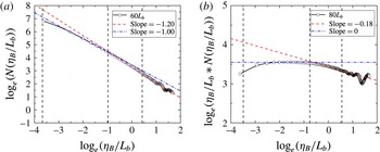
Time-averaged number $N(\unicode[STIX]{x1D702}_{B})$ of squares of side size $\unicode[STIX]{x1D702}_{B}$ needed to cover the TNT interfacial line in the 2-D plane $x/L_{b}=60$ versus $\unicode[STIX]{x1D702}_{B}/L_{b}$ (a) and $\unicode[STIX]{x1D702}_{B}N(\unicode[STIX]{x1D702}_{B})$ versus $\unicode[STIX]{x1D702}_{B}/L_{b}$ for the 2-D plane $x/L_{b}=80$ (b). The $\ln -\ln$ plots (a) and (b) are given for different streamwise positions to give an impression of variability. The fractal dimension is well defined over one decade and found to equal $6/5\pm 0.02$ in the range $x/L_{b}=50$ to $x/L_{b}=100$ . The values $\unicode[STIX]{x1D702}_{B}=\unicode[STIX]{x1D702}_{K}$ , $\unicode[STIX]{x1D706}$ and $\unicode[STIX]{x1D6FF}$ are indicated in the plots for reference.

3.2 DNS results: fractal nature of the TNT interface and $\unicode[STIX]{x1D702}_{I}\sim \unicode[STIX]{x1D708}/v_{n}$

We now test the assumption that the intersection of the TNT interface with a $y$ – $z$ plane is a fractal line over some range of length scales. To test this assumption we use the well-known box-counting algorithm (Mandelbrot Reference Mandelbrot1982; Sreenivasan et al. Reference Sreenivasan, Ramshankar and Meneveau1989; Mistry et al. Reference Mistry, Philip, Dawson and Marusic2016) and count the number of squares of side size $\unicode[STIX]{x1D702}_{B}$ required to cover the TNT interfacial line in the 2-D plane. We repeat this counting for approximately one-fifth of all our time samples and then calculate the average number of such squares of size $\unicode[STIX]{x1D702}_{B}$ . This average number is $N(\unicode[STIX]{x1D702}_{B})$ and it is obtained for a range of $\unicode[STIX]{x1D702}_{B}$ values from $\unicode[STIX]{x1D702}_{K}$ to a few times $\unicode[STIX]{x1D6FF}$ . An example of the outcome of this procedure is given in figure 4(a).

For all the 2-D planes between $x/L_{b}=50$ and $100$ tried here, there is a well-defined range of sizes $\unicode[STIX]{x1D702}_{B}$ where $N(\unicode[STIX]{x1D702}_{B})$ can be fitted as $N(\unicode[STIX]{x1D702}_{B})=N_{\unicode[STIX]{x1D6FF}}(\unicode[STIX]{x1D702}_{B}/\unicode[STIX]{x1D6FF})^{-D}$ with $D>1$ . The exponent $D$ is the fractal dimension of the TNT interfacial line in the 2-D $y$ – $z$ plane and we find it to be equal to $6/5\pm 0.02$ at all the streamwise locations that we have interrogated (see figure 4). At smaller length scales $\unicode[STIX]{x1D702}_{B}$ , the dimension $D$ is close to 1 as it should be. This finding supports the assumption that the TNT interfacial line is fractal in every 2-D lateral plane between $x/L_{b}=50$ and $100$ . Its non-integer fractal dimension is defined over a range of scales which spans one decade. (We checked that the TNT interface is equally wrinkled in parts of $x-y$ and $x-z$ planes extending from $x/L_{b}=50$ to $x/L_{b}=100$ by confirming that the fractal dimension of the TNT interfacial line in such planes is also well defined over an equally broad range of scales and also equal to $6/5\pm 0.02$ .)

Even though $D=6/5\pm 0.02$ irrespective of streamwise position in the streamwise range tested, $N_{\unicode[STIX]{x1D6FF}}$ varies significantly with $x$ if we keep the value of $\unicode[STIX]{x1D714}_{th}/\unicode[STIX]{x1D714}_{max}$ the same for all our 2-D planes (the same happens when we use $\unicode[STIX]{x1D714}_{th}/\unicode[STIX]{x1D714}_{av}$ or $\unicode[STIX]{x1D714}_{th}/\overline{\unicode[STIX]{x1D714}}(x,0,0)$ instead of $\unicode[STIX]{x1D714}_{th}/\unicode[STIX]{x1D714}_{max}$ ). There is no irrefutable reason why the downstream evolution of the interface should be traced with the same threshold $\unicode[STIX]{x1D714}_{th}/\unicode[STIX]{x1D714}_{max}$ (or $\unicode[STIX]{x1D714}_{th}/\unicode[STIX]{x1D714}_{av}$ or $\unicode[STIX]{x1D714}_{th}/\overline{\unicode[STIX]{x1D714}}(x,0,0)$ ) at all streamwise positions $x$ . The dynamics of the interfacial region is actually such that the normalised threshold range over which the time-averaged area $A$ has a plateau in figure 1(b) varies a little with $x$ and $\unicode[STIX]{x1D714}_{max}$ varies with both time and $x$ too. 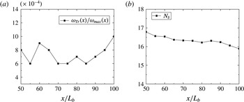However, $N_{\unicode[STIX]{x1D6FF}}$ should remain constant with $x$ for a self-similar turbulent wake. We therefore identify a set of different normalised thresholds $\unicode[STIX]{x1D714}_{th}/\unicode[STIX]{x1D714}_{max}$ for different streamwise positions, see figure 5(a), for which $N_{\unicode[STIX]{x1D6FF}}$ is approximately constant, see figure 5(b). These normalised thresholds are all within the minimal range $4\times 10^{-4}$ and $7\times 10^{-3}$ which is part of the range where $A$ has a plateau for any $x/L_{b}$ between $50$ and $100$ . We have checked that the value of $D$ remains within $6/5\pm 0.02$ with these thresholds. (The results are effectively the same if $\unicode[STIX]{x1D714}_{th}/\unicode[STIX]{x1D714}_{av}$ or $\unicode[STIX]{x1D714}_{th}/\overline{\unicode[STIX]{x1D714}}(x,0,0)$ is used instead of $\unicode[STIX]{x1D714}_{th}/\unicode[STIX]{x1D714}_{max}$ with a similar variation in $\unicode[STIX]{x1D714}_{th}/\unicode[STIX]{x1D714}_{av}$ and $\unicode[STIX]{x1D714}_{th}/\overline{\unicode[STIX]{x1D714}}(x,0,0)$ by a factor of approximately less than 2 but different actual values for $\unicode[STIX]{x1D714}_{th}/\unicode[STIX]{x1D714}_{av}$ or $\unicode[STIX]{x1D714}_{th}/\overline{\unicode[STIX]{x1D714}}(x,0,0)$ .)

Figure 5.

Choice of thresholds $\unicode[STIX]{x1D714}_{th}/\unicode[STIX]{x1D714}_{max}$ ((a) as a function of $x/L_{b}$ ) so that $N_{\unicode[STIX]{x1D6FF}}$ ((b) as a function of $x/L_{b}$ ) remains approximately constant with $x$ .

The fractal nature of the TNT interfacial line enters the theoretical considerations of § 2 via the length ${\mathcal{L}}$ in (2.2) and (2.3). We therefore calculate an estimate of the time-averaged interfacial length at resolution $\unicode[STIX]{x1D702}_{B}$ . This is $L(\unicode[STIX]{x1D702}_{B})=\unicode[STIX]{x1D702}_{B}N(\unicode[STIX]{x1D702}_{B})$ and an example is given in figure 4(b). A maximum value of $\ln L(\unicode[STIX]{x1D702}_{B})$ is clearly visible in figure 4(b) and it is present at all streamwise positions. This maximum demarcates the scales $\unicode[STIX]{x1D702}_{B}$ which are small enough to resolve the line as a set of points from the scales $\unicode[STIX]{x1D702}_{B}$ which are large enough for the line to be perceived as continuous. We take this maximum value of $L(\unicode[STIX]{x1D702}_{B})$ to be the actual time-averaged length of the interface ${\mathcal{L}}$ . 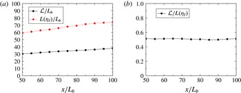(We verified this way of estimating ${\mathcal{L}}$ against a way based on the marching squares algorithm, fully independently of the box-counting algorithm, and found good agreement.) In figure 6(a) we plot ${\mathcal{L}}(x)/L_{b}$ as a function of $x/L_{b}$ . We find, as expected, that ${\mathcal{L}}$ is an increasing function of $x$ .

Equation (2.3) in § 2 follows from ${\mathcal{L}}\sim L(\unicode[STIX]{x1D702}_{B})$ for $\unicode[STIX]{x1D702}_{B}=\unicode[STIX]{x1D702}_{I}$ . Indeed, ${\mathcal{L}}\sim L(\unicode[STIX]{x1D702}_{I})=\unicode[STIX]{x1D702}_{I}N(\unicode[STIX]{x1D702}_{I})$ , $N(\unicode[STIX]{x1D702}_{I})=N_{\unicode[STIX]{x1D6FF}}(\unicode[STIX]{x1D702}_{I}/\unicode[STIX]{x1D6FF})^{-D}$ and $N_{\unicode[STIX]{x1D6FF}}=\text{const.}$ yield (2.3). But the other important assumption in § 2 is that ${\mathcal{L}}\sim L(\unicode[STIX]{x1D702}_{I})$ with $\unicode[STIX]{x1D702}_{I}\sim \unicode[STIX]{x1D708}/v_{n}$ . To verify this assumption, we calculate $v_{n}$ from (2.2) with ${\mathcal{L}}$ estimated as described in the previous paragraph. We then calculate $L(\unicode[STIX]{x1D702}_{I})=\unicode[STIX]{x1D702}_{I}N(\unicode[STIX]{x1D702}_{I})=N_{\unicode[STIX]{x1D6FF}}\unicode[STIX]{x1D6FF}(\unicode[STIX]{x1D702}_{I}/\unicode[STIX]{x1D6FF})^{1-D}$ with $\unicode[STIX]{x1D702}_{I}=\unicode[STIX]{x1D708}/v_{n}$ and compare it to ${\mathcal{L}}$ . The results of this comparison are given in figure 6. We find that ${\mathcal{L}}/L(\unicode[STIX]{x1D702}_{I})$ is approximately constant with $x$ , in support of the way we use $\unicode[STIX]{x1D702}_{I}\sim \unicode[STIX]{x1D708}/v_{n}$ .

In conclusion, our DNS supports all the assumptions made in § 2, in particular $A\sim \unicode[STIX]{x1D6FF}^{2}$ (as shown in § 3.1) and ${\mathcal{L}}\sim \unicode[STIX]{x1D6FF}(\unicode[STIX]{x1D702}_{I}/\unicode[STIX]{x1D6FF})^{1-D}$ with $\unicode[STIX]{x1D702}_{I}\sim \unicode[STIX]{x1D708}/v_{n}$ . The actual value of $\unicode[STIX]{x1D702}_{I}$ for which ${\mathcal{L}}$ is equal (rather than just proportional) to $L(\unicode[STIX]{x1D702}_{I})$ is a value close to $\unicode[STIX]{x1D706}$ as can be inferred from figure 4. However, $\unicode[STIX]{x1D702}_{I}$ does not scale with $\unicode[STIX]{x1D706}$ (nor does it scale with $\unicode[STIX]{x1D702}_{K}$ ) but with $\unicode[STIX]{x1D708}/v_{n}$ . We checked that $(\unicode[STIX]{x1D708}/v_{n})/\unicode[STIX]{x1D706}$ and $(\unicode[STIX]{x1D708}/v_{n})/\unicode[STIX]{x1D702}_{K}$ are not constant and in fact vary significantly with $x$ . The range of length scales where the TNT interfacial line in the 2-D planes $x/L_{b}=50{-}100$ is fractal is bound from below by an inner length scale proportional to $\unicode[STIX]{x1D708}/v_{n}$ and from above by a multiple of $\unicode[STIX]{x1D6FF}$ .

Figure 6.

${\mathcal{L}}/L_{b}$ and $L(\unicode[STIX]{x1D702}_{I})/L_{b}$ (a) and ${\mathcal{L}}/L(\unicode[STIX]{x1D702}_{I})$ (b) versus $x/L_{b}$ . The TNT interfacial line is defined with the thresholds given in figure 5(a) and $\unicode[STIX]{x1D702}_{I}=\unicode[STIX]{x1D708}/v_{n}$ where $v_{n}$ is calculated from (2.2).

3.3 DNS results: Kolmogorov and local entrainment velocities

Having found DNS support for the assumptions made in § 2 we now use our DNS to assess the main results of the theoretical arguments in that section, namely (2.8) and (2.9). As shown by Dairay et al. (Reference Dairay, Obligado and Vassilicos2015), the dissipation scaling in the range $x/L_{b}=50{-}100$ of the axisymmetric turbulent wake of our DNS is such that $m=1/2$ which means that we need to assess (2.8) and (2.9) against our DNS results with $\unicode[STIX]{x1D6FE}_{e}=3/7+1/(7D)$ for (2.8) and $\unicode[STIX]{x1D6FE}_{\unicode[STIX]{x1D702}}\approx 0.607$ for (2.9) (see table 1). Indeed, $m=1/2$ implies $\unicode[STIX]{x1D6FD}=3/7$ which implies $\unicode[STIX]{x1D6FE}_{e}=(\unicode[STIX]{x1D6FD}(D-1))/D+(1-\unicode[STIX]{x1D6FD})/D=3/7+1/(7D)$ and $\unicode[STIX]{x1D6FE}_{\unicode[STIX]{x1D702}}=(\unicode[STIX]{x1D6FD}(1+m))/4+((3-m)/8)(\unicode[STIX]{x1D6FD}+1)\approx 0.607$ .

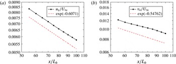
Figure 7(a) shows that the DNS returns an $x$ -dependence of $u_{\unicode[STIX]{x1D702}}/U_{\infty }$ which is in good agreement with (2.9) and $\unicode[STIX]{x1D6FE}_{\unicode[STIX]{x1D702}}=0.607$ in the range $x/L_{b}=50{-}100$ . However, as can be seen in figure 7(b), the agreement between (2.8) with $\unicode[STIX]{x1D6FE}_{e}=(\unicode[STIX]{x1D6FD}(D-1))/D+(1-\unicode[STIX]{x1D6FD})/D=3/7+1/(7D)=0.5476$ (for $D=6/5$ ) and the DNS is less good even though the decreasing downstream nature of $v_{n}/U_{\infty }$ is well captured and is not too far from the data. These data have been produced by calculating the local entrainment velocity $v_{n}$ from (2.2), (2.5) and the previous subsection’s DNS estimate of ${\mathcal{L}}$ . The agreement with (2.8) where $\unicode[STIX]{x1D6FE}_{e}=0.5476$ cannot be expected to be too good given that $D$ varies around $6/5$ from one streamwise position to the other and given the uncertainty on how to exactly follow the TNT interfacial line in terms of vorticity thresholds from one streamwise position to the other. 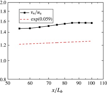Even so, the prediction that $v_{n}/u_{\unicode[STIX]{x1D702}}$ is not constant but a very slowly increasing function of $x$ is supported by our DNS (see figure 8).

Figure 7.

$u_{\unicode[STIX]{x1D702}}/U_{\infty }$ (a) and $v_{n}/U_{\infty }$ (b) versus $x/L_{b}$ . For comparison the dotted line in (a) represents the power-law dependence on $x$ given by (2.9) with $\unicode[STIX]{x1D6FE}_{\unicode[STIX]{x1D702}}\approx 0.607$ and the dotted line in (b) represents the power-law dependence on $x$ given by (2.8) with $\unicode[STIX]{x1D6FE}_{e}=3/7+1/(7D)$ and $D=6/5$ .

Figure 8.

$v_{n}/u_{\unicode[STIX]{x1D702}}$ versus $x/L_{b}$ . For comparison the dotted line represents $(x-x_{0})^{\unicode[STIX]{x1D6FE}_{\unicode[STIX]{x1D702}}-\unicode[STIX]{x1D6FE}_{e}}=(x-x_{0})^{0.059}$ which is the $x$ -dependence predicted for $v_{n}/u_{\unicode[STIX]{x1D702}}$ from (2.8) and (2.9) if $m=1/2$ , $D=6/5$ and $x_{0}$ is the same virtual origin as the one in (2.5) and (2.6).

4 Conclusion and discussion

It is not always true that the local entrainment velocity $v_{n}$ scales with the Kolmogorov velocity $u_{\unicode[STIX]{x1D702}}$ . As we have argued in this paper, this depends on the turbulence dissipation scalings, at least in the case of self-similar axisymmetric turbulent wakes.

Recent studies have shown that the local entrainment velocity scales with the Kolmogorov velocity and that the thickness of the TNT interface scales with the Kolmogorov length scale in some turbulent flows (Holzner & Lüthi Reference Holzner and Lüthi2011; Watanabe et al. Reference Watanabe, Sakai, Nagata, Ito and Hayase2015, Reference Watanabe, Riley, de Bruyn Kops, Diamessis and Zhou2016). This conclusion may have been reached because the regions of the flows studied are such that the turbulence dissipation scalings are classical, as one may for example expect extremely far downstream in a turbulent wake (Redford et al. Reference Redford, Castro and Coleman2012), or because the effect can be imperceptible (see figure 8), as in nearer field axisymmetric self-similar turbulent wakes when the Reynolds number is not high enough.

Our DNS study has concentrated in a region of a turbulent wake where the turbulent flow is statistically axisymmetric and self-similar and where the dissipation scalings are given by (2.7) with $m=1/2$ . We have presented theoretical arguments which demonstrate that the local entrainment velocity and the thickness of the TNT interface do indeed scale with the Kolmogorov velocity and length scale respectively when $m=0$ . This is the dissipation scaling usually considered, for example in textbooks (e.g. Tennekes & Lumley Reference Tennekes and Lumley1972; Townsend Reference Townsend1976; Pope Reference Pope2000). However, the same theoretical arguments lead to the conclusion that $v_{n}$ does not scale with $u_{\unicode[STIX]{x1D702}}$ when $m\not =0$ and that $v_{n}$ has the same dependence on downstream streamwise distance as $\unicode[STIX]{x1D708}/\unicode[STIX]{x1D706}$ when $m=1$ even though it has a different dependence on global Reynolds number. The case $m=1$ corresponds to the non-equilibrium dissipation scaling found in various turbulent flows at high enough Reynolds numbers (Goto & Vassilicos Reference Goto and Vassilicos2015; Vassilicos Reference Vassilicos2015; Obligado et al. Reference Obligado, Dairay and Vassilicos2016).

Our theoretical arguments have been based on the idea, already present in Corrsin & Kistler (Reference Corrsin and Kistler1955), that interfacial statistics scale with the wake width $\unicode[STIX]{x1D6FF}(x)$ and in particular that the time-averaged area $A$ of the fully turbulent region in a plane normal to the mean direction of the flow scales with $\unicode[STIX]{x1D6FF}^{2}$ . Our DNS data have provided good support for $A\sim \unicode[STIX]{x1D6FF}^{2}$ in the range $50\leqslant x/L_{b}\leqslant 100$ . This is the first time that such a result has been obtained by any means, whether experimental or numerical. We have also shown that the PDF of the radial interface location is self-similar and scales with $\unicode[STIX]{x1D6FF}$ , at least in that range. This kind of result finds its roots in Corrsin & Kistler (Reference Corrsin and Kistler1955) and has been verified in various flows since then, such as turbulent jets (Watanabe et al. Reference Watanabe, Sakai, Nagata, Ito and Hayase2014; Mistry et al. Reference Mistry, Philip, Dawson and Marusic2016) and turbulent mixing layers (Attili, Cristancho & Bisetti Reference Attili, Cristancho and Bisetti2014) but this is the first time that it has been obtained in a DNS of a spatially evolving turbulent wake. Furthermore, we find that the PDF of the radial interface location is approximately Gaussian in our flow, in agreement with the original suggestion by Corrsin & Kistler (Reference Corrsin and Kistler1955) and with similar findings in various other turbulent flows including time-evolving wakes (Bisset, Hunt & Rogers Reference Bisset, Hunt and Rogers2002), turbulent boundary layers (Chauhan et al. Reference Chauhan, Philip, de Silva, Hutchins and Marusic2014; Borrell & Jiménez Reference Borrell and Jiménez2016), turbulent jets (Westerweel et al. Reference Westerweel, Fukushima, Pedersen and Hunt2009; Gampert et al. Reference Gampert, Kleinheinz, Peters and Pitsch2014; Watanabe et al. Reference Watanabe, Sakai, Nagata, Ito and Hayase2014; Mistry et al. Reference Mistry, Philip, Dawson and Marusic2016) and turbulent mixing layers (Attili et al. Reference Attili, Cristancho and Bisetti2014).

The other important assumption of our theoretical arguments is that the TNT interfacial line in 2-D planes normal to the mean direction of the flow has fractal properties. Our DNS has provided support for this assumption and has returned a fractal dimension $D=6/5\pm 0.02$ at the streamwise locations $x/L_{b}=50{-}100$ where our DNS study has concentrated attention. The DNS results also support the scaling of the relevant inner length scale $\unicode[STIX]{x1D702}_{I}$ with $\unicode[STIX]{x1D708}/v_{n}$ , somehow echoing the arguments of Corrsin & Kistler (Reference Corrsin and Kistler1955).

It is interesting that $D$ is appreciably different from the more usual value $4/3$ which follows from a Kolmogorov scaling of the TNT interface (see paragraph under (2.9) in § 2). This finding is consistent with the non-Kolmogorov scalings of the TNT interface when $m\not =0$ . In the flow region studied by our DNS, $m=1/2$ . In the same flow region, $m=1$ when the Reynolds number is sufficiently higher (see Dairay et al. Reference Dairay, Obligado and Vassilicos2015; Vassilicos Reference Vassilicos2015; Obligado et al. Reference Obligado, Dairay and Vassilicos2016).

In the DNS of Redford et al. (Reference Redford, Castro and Coleman2012) and Goto & Vassilicos (Reference Goto and Vassilicos2016) and the wind tunnel experiments of Valente & Vassilicos (Reference Valente and Vassilicos2012, Reference Valente and Vassilicos2014) the dissipation scaling morphs quite suddenly from $m=1$ to $m=0$ far enough downstream. The DNS of decaying periodic turbulence of Goto & Vassilicos (Reference Goto and Vassilicos2016) suggest that this happens when the large-scale coherent structures weaken enough for their presence to stop affecting turbulence statistics significantly. This suggests that different local TNT interface scalings for $v_{n}$ and $\unicode[STIX]{x1D702}_{I}$ may exist in the presence or absence of engulfment (see Corrsin & Kistler Reference Corrsin and Kistler1955; da Silva et al. Reference da Silva, Hunt, Eames and Westerweel2014), and that engulfment may be closely related to non-equilibrium turbulence cascade and associated dissipation scaling exponents $m\not =0$ , in particular $m=1$ , whereas the prevalence of nibbling (see Corrsin & Kistler Reference Corrsin and Kistler1955; da Silva et al. Reference da Silva, Hunt, Eames and Westerweel2014) may be associated with the usual dissipation scaling exponent $m=0$ . We are currently pursuing this new research direction and hope to report on it soon.