

1. Introduction
Information on the characteristics of the demand for money is crucial to understanding the evolution of price levels. However, good-quality time series of the variables needed to estimate money demand (such as interest rates, income, wealth) are scarce for any economy prior to the nineteenth century. For this reason, the vast majority of economic historians tried to explain the evolution of prices in pre-industrial Europe by using the Fisher identity (MV = PT) and suggesting hypotheses about what part of the changes in price levels (P) can be assigned to changes in the stock of money (M), the amount of transactions (T), or the velocity of circulation (V).
One important problem with using the Fisher identity in the context of the economic history of modern Europe is that, although there is plenty of reliable information concerning prices, there is little information about T, an incomplete and unreliable series of M, and basically nothing about V (which is usually calculated as a residual once the series of the other three variables are constructed). This implies that − for the entire period between the start of the fifteenth and the first half of the nineteenth century − Fisher's identity can be applied to only a few benchmark years and with wide margins of error. This restricts the analysis of price determination to the level of controlled conjectures (Lindert Reference Lindert1985; Mayhew Reference Mayhew1995).
Another problem with relying only on Fisher's equation to explain the evolution of price levels is that, even if we have reliable time series of the four variables in the equation, it remains difficult to pin down the final determinants of changes in V.Footnote 1 If V is set independently of the other variables of the equation, then the equation M/P = 1/V × T can be considered a demand for money.Footnote 2 This is why changes in the demand for money in modern Europe have usually been linked to changes in total marketed output (T) and to changes in the velocity of circulation (V) (Goldstone Reference Goldstone1984, Reference Goldstone1991). On the one hand, total marketed output would have been affected by relatively well-known processes (population size, degree of specialization, market structure, etc.) and we know that the higher the marketed output, the higher the demand for money. In this case, a relatively more complex economy with a larger tertiary sector would have a higher demand for money because specialization would be higher. On the other hand, the higher the velocity, the lower the demand for money holdings because a smaller amount of money can be used for the same level of transactions. Yet the reasons behind the changes in V are still far from clear. For instance, there is debate about the impact of urbanization on the velocity of circulation: some authors (e.g. Goldstone Reference Goldstone1984) believe that larger cities would have induced more frequent transactions and therefore smaller money holdings, whereas others (e.g. Mayhew Reference Mayhew1995) suggest that urbanization would have increased the opportunities to use money and thus the incentives to hold cash.
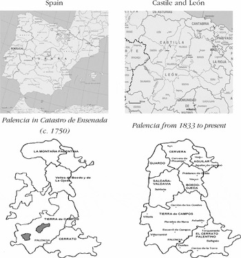
In this article we suggest a novel methodological alternative in order to improve our understanding of monetary phenomena in pre-industrial Europe. The methodology is based on probate inventories, a well-known source that is widely available for different periods and regions in pre-industrial Europe.Footnote 3 Probate inventories have been used to analyse a variety of issues, including wealth distribution, consumption patterns, agricultural practices, characteristics of informal credit markets, and more. Focusing on a set of probate inventories from eighteenth-century Palencia, Spain (see Figure 1), we show that it is possible to estimate a money demand (the first ever estimated for a pre-industrial economy) by relying on several types of information about the deceased person: the money held in cash, financial assets, wealth, age, place of residence (urban or rural) and the economic sector in which the person worked. Following Mulligan and Sala-i-Martín (Reference Mulligan and Sala-i-Martín1992), we devise a cross-section estimate of the money demand that sheds new light on (i) the relationship between wealth and money demand, which can provide important insights into the impact of economic growth on price levels through the change in the level of desired money holdings; and (ii) the validity of some hypotheses about the relation between price levels, money holdings, and non-monetary processes like urbanization and structural change. Our sample is admittedly rather small and covers only a limited period of the eighteenth century. Nonetheless, our approach provides empirically tested results that are relevant to any discussion or hypothesis concerning pre-industrial monetary phenomena and that suggest a new methodology for future research.
Palencia, 1700–1800

The rest of the article is organized as follows. Section 2 briefly reviews the debate over the causes of inflation in pre-industrial economies as well as the debate's underlying assumptions about the money demand. In Section 3 we characterize the economic situation of Palencia (from a comparative perspective) during the eighteenth century. Section 4 describes the process of systematizing the information contained in probate inventories and how these data have been combined with census information from the Catastro de Ensenada to solve potential problems of selection bias. In Section 5 we present our econometric strategy for estimating the demand for money and also the implications of the results. Finally, Section 6 concludes. At the end are the tables with the results as well as an appendix that contains analyses of the implications of some assumptions made in the article.
2. Previous approaches
Most of the debate about what determined price levels in pre-industrial Europe is related in one way or another to the ultimate causes of the sixteenth-century Price Revolution. Probably the first milestone in this debate is the work by Hamilton (Reference Hamilton1934), who hypothesized that inflation in Spain and the rest of Europe during the sixteenth and seventeenth centuries was caused by the inflow of precious metals from America and their diffusion throughout Europe. This hypothesis is based on Fisherian quantity theory (MV = PT), and it is argued that the increase in M fostered by imports of American silver was a much greater factor in inflation than was any change in the velocity of circulation or in real output.Footnote 4
Goldstone (Reference Goldstone1984, Reference Goldstone1991) downplays the role of M and instead proposes an explanation focused on T (level of transactions) and on V (velocity of circulation). His population- and velocity-based explanation states that population growth induced urbanization and specialization between 1500 and 1650 and that these processes should, in turn, have implied not only more transactions (which should have reduced prices) but also − and more importantly − a much higher velocity of circulation (which should have increased prices). In this view, the increase in M is not enough to explain the increase in P once the increase in T is taken into account. Consequently, the increase in prices must result mainly from significant growth in V. Goldstone's hypothesis relies on the relationship between population's density and the complexity of its networks (and the resulting number of links). Empirical support for this hypothesis is, unfortunately, both indirect and inconclusive.
Lindert (Reference Lindert1985) analyses the possible links between population growth (and its connections with velocity in Fisher's equation) and the changes in prices in England between the sixteenth and the nineteenth century. He explicitly uses Fisher's equation and endorses, at least partially, the Goldstone hypothesis regarding the links between population density, urbanization, velocity and price levels. However, Lindert recognizes also that it is difficult to establish a clear-cut link between some historically observed processes (such as population growth, urbanization and institutional change) and any of the equation's variables.Footnote 5
Flynn (Reference Flynn, Irsigler and Cauwenberghe1984) and Doherty and Flynn (Reference Doherty, Flynn and Cauwenberghe1989) argue that the Fisherian approach is difficult to handle in a precise way. These authors claim that the approach is wrong in making an artificial distinction between active and passive money and also that it confuses stocks with flows: whereas Fisher's equation is based on a flow approach (what matters is money in circulation), modern monetary economics is based on stocks (what matters is money holdings at a given moment in time). In this context, Flynn and Doherty insist that price determination depends on the interaction between supply and demand of money stocks; they concede, however, that estimating the demand for money stock is extremely difficult with the data currently available.
Mayhew (Reference Mayhew1995) suggests that V declined sharply in England between 1561 and 1643, so he rejects any association of urbanization and commercialization with a rising V. Mayhew explains this view by discussing the difference between V and the concept of k from the Cambridge school: ‘In truth V is far more likely to fall with the increasing use of money than to rise. The Cambridge school of economics understood this well when they preferred to use the concept of k, the demand for money to hold, instead of V. An increase in the use of money entails a rise in the demand for money and therefore a fall in V (since k is the inverse of V).’
So, until recently, the use of Fisher's equation and the Cambridge approach has been pervasive in the debate surrounding prices in pre-industrial Europe. In this context, any discussions about consequences for the price level of changes in the demand for money should be necessarily focused on (and limited to) changes in k or V.Footnote 6 However, the lack of reliable and consistent data on money stocks makes it impossible to obtain reliable estimates of V; hence scholars have so far been limited to venturing educated guesses about its determinants. Although we have important reasons to believe that economic growth, structural change, population growth and urbanization (among other factors) affect the demand for money holdings and consequently the price level, assessing the direction and magnitude of the effects is virtually impossible with the available data.
In the sections that follow we will suggest that the analysis of probate inventories can be extremely helpful in understanding the determinants of money holdings. Although our example comes from Palencia, a relatively small area in the north of Spain, we argue that it provides an important methodological innovation for assessing and understanding of the effects of urbanization, structural change and economic growth on the demand for money and on price levels.
3. Economic structure and monetary system of eighteenth-century Palencia
In this section, we summarize the main features of the Palencian economy in order to characterize the context in which the households of our data set developed their daily activities. In several dimensions, Palencia was quite standard: its demographic characteristics, its economic structure and its welfare levels do not seem to be much different from those of other areas in modern Europe. The monetary system in Palencia was the one defined by the Spanish crown for all the Castilian territory.
In the second half of the eighteenth century, Palencia had a population of about 120,000 and a relatively high population density: in this it was tenth among the Spanish provinces.Footnote 7 The most populated municipalities in Palencia (1787) were: Palencia (10,345 inhabitants in 1787), Paredes de Nava (3,926 inhabitants) and Villarramiel (2,003 inhabitants).Footnote 8
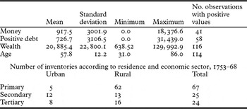
Chronicles of the time classified Palencia as ‘the most industrious province of Castile’ (Larruga 1787). Available data for the working population show that between 60 and 75 per cent of those who live in the city of Palencia were working in the secondary and tertiary sector. According to the Catastro de Ensenada, about 3,000 people based around the La Puebla district of the city − of a total population of more than 9,000 inhabitants − worked in one of the various stages of the textile manufacturing process.Footnote 9 In contrast, in the rural areas this percentage barely rose above 30 per cent because there were few connections between productive processes of the ‘unionized’ urban industry and those of the scattered rural industry (Yun Reference Yun Casalilla1987). In general terms, the region of Tierra de Campos and, to a lesser extent, the Cerrato Palentino (located to the south of Palencia) had quite important secondary and tertiary sectors. In contrast, agricultural and livestock activities were practically the only sources of wealth in the regions of the northern half of the province (except in the valleys of Boedo and La Ojeda, which were of great importance to the local cheap textile industry). The distribution of individuals in our sample fits this pattern quite well: 80 per cent of urban individuals were engaged in activities from the secondary and tertiary sectors; and 68 per cent of those living in rural areas worked in agriculture (see Table 1).
Summary statistics of main variables

Standards of living in Palencia in the second half of the eighteenth century were probably not markedly higher or lower than in other parts of modern Europe. Between 1750 and 1800, the nominal wages of bricklayers in the city of Palencia were similar to those of peones in Madrid (Moreno Reference Moreno and Martínez2002; Hamilton 1947). The absence of comparable price indexes precludes a precise comparison of real wages, but if we assume that price levels differed little between the two cities then real wages should also be fairly alike.Footnote 10 According to Allen (Reference Allen2001), workers’ welfare in Madrid in the second half of the eighteenth century was lower than in other important pre-industrial European cities but was not unusually low: the welfare ratio of building craftsmen in Madrid during 1750–99 was just 63 per cent of the average measured in London between 1500 and 1800 (the second highest in Europe after Antwerp), yet it was 90 and 95 per cent of that average in Milan/Florence and Paris, respectively.Footnote 11 Although the comparison is quite crude, it does suggest that, in the context of pre-industrial Europe, the region of Palencia was not an outlier in terms of standards of living.
During the sixteenth and seventeenth centuries, each political unit within the Kingdom of Spain (Castile, Navarra and Aragon) had its own monetary system. In the first half of the eighteenth century, the Borbones made important efforts to create a unified monetary system based on three different types of coins: the onza, made with gold; the real de a ocho or peso fuerte, made with silver; and the maravedí and the real de vellón, made with bronze. One peso fuerte was equivalent to 640 maravedís, and one real de vellón was equivalent to 34 maravedís. The onza and the real de a ocho were used for large transactions (usually related to international trade) whereas the real de vellón and the maravedí were standard units of account and the typical means of payment for domestic and smaller transactions.
Even though the Spanish colonies in America were the most important producers of silver in the globe, the peso was rather unusual in eighteenth-century Spain, most of whose internal circulation was denominated in maravedí or reales de vellón. This was so because the value of silver relative to gold in Spain (1 to 16) was slightly higher than elsewhere in Europe (1 to 15.5 in France; 1 to 15.2 in England) and much higher than in India and China (1 to 10 and 1 to 12, respectively). As long as low transport costs created the opportunity for arbitrage, coins with high silver content were exported.Footnote 12
The quantity of money in circulation in Spain in the eighteenth century is extremely difficult to determine. Sardá (Reference Sarda1998) estimated that between 10,000 and 15,000 million reales de vellón could have been imported by Spain during the eighteenth century. Canga Argüelles (Reference Canga Argüelles1833) reported that, between 1793 and 1797, 145 million reales de vellón were imported from America to the public system of ‘Hacienda Pública’ in peninsular Spain. How much of this money remained in Spanish circulation? In 1782 a general re-coinage was imposed by Carlos III, but by 1792 a mere 1,269 million reales de vellón had passed through the royal mints. According to Sardá, at the beginning of nineteenth century, the total amount of money in circulation could not have exceeded 4,000 million reales, and most of this would probably be smaller coins with low metallic content.Footnote 13
4. Data from probate inventories and the Catastro de Ensenada
A probate inventory is a comprehensive list of all the goods owned by the deceased at the time of death, and it was usually made by a scribe and certified by a notary or judicial authority within a few days. The historical research in several fields utilizes probate inventories because they are relatively abundant in archives worldwide and include a wide variety of information. Braudel (Reference Braudel1967) declared that probate inventories were truthful documents (documents de vérité) because they contain reliable data about daily life in household economies. This characteristic has contributed to our knowledge of urban domestic spaces (Brown Reference Brown1986; Bedell Reference Bedell2000), to advances in cultural history and history of social identities (Bermingham and Brewer Reference Bermingham and Brewer1995), and to economic history. In the latter discipline, Thirsk (Reference Thirsk1978), Overton (Reference Overton1979, Reference Overton, der Woude and Schuurman1980, Reference Overton and Reed1984, Reference Overton, Mathias and Davis1996), Overton and Campbell (Reference Overton and Campbell1992) and Allen (Reference Allen1988), among others, have used inventories in the studies of agrarian history, agricultural practices, livestock husbandry developments, and productivity levels. Lindert (Reference Lindert1980) has analysed English occupational composition on the eve of the Industrial Revolution combining information from burial registers and probate inventories. Other authors − such as Holderness (Reference Holderness1976), Groves (Reference Groves1994) and Muldrew (Reference Muldrew1998) − have used probate inventories to analyse financial strategies of families and the functioning of informal credit markets.
At the beginning of the 1980s, a number of historians emphasized the importance of consumption in explaining the spreading of the Industrial Revolution; see Thirsk (Reference Thirsk1978) and McKendrick (Reference McKendrick, McKendrick, Brewer and Plumb1982) for the English case and Roche (1989) for the French case. Thereafter, a number of investigations into the history of consumption and the study of the material culture were carried out using probate inventories. In this regard, the studies of Weatherill (Reference Weatherill1988) for England and of Shammas (Reference Shammas1990) for England and the North American colonies stand out. Later, de Vries (Reference Vries, Brewer and Porter1993) pointed out the apparent paradox of the decrease in family purchasing power (via wages) and the growth in domestic consumption as evidenced by probate inventories; using the same source, King (Reference King, Hitchcock, King and Sharpe1997) has confirmed the growth in the stock of durable consumption goods among the English paupers during the eighteenth century. In the Spanish case, Torras and Yun (Reference Torras Elías and Yun Casalilla1999) have studied consumption patterns, commercialization networks, and the standard of living in a pre-industrial society by examining post-mortem inventories and dowries.
In Castile, all possessions of the deceased were officially recorded in a notarized document (protocolo notarial) that included signatures of the scribe, the notary, the witnesses and the appearing parties. Sometimes the inventory included a will that had been previously written and signed by the deceased. At the beginning of the inventory, the place and the date of the document's elaboration are noted together with a list of the persons involved: mainly the designated official, the inheritors and their legal advisors. One inventory in our data set starts with the following description:
In the town of Palencia, on the 14 of September 1755, joined together to make and finalize the settlement, counting and division of the assets and credits, belonging to Mr Felipe Ortega, who was an inhabitant of this town, are Messrs. José Cavezon, town clerk, as the executor, with full authority for this division; Mrs María Alonso, his widow, legatee of half of the third share; Juana, his daughter and inheritor, and Alejandro, his son and inheritor, all of whom are inhabitants of this town and of legal age.Footnote 14
This kind of preamble is followed by a list of all goods along with the valuation of each. The listing often begins with the value of the house followed by the different items present in each room of the house: furniture, equipment, books, decorative objects and so forth. For instance, in the probate inventory of Bernardo Castro, farmer and woollen maker (fabricante de paños) from Prádanos de Ojeda, we find the following items: two chests and coffers (arcas), valued at 4 and 5 reales, respectively; five beds with values ranging from 12 to 40 reales; two candlesticks (8 reales each); four plates (20 reales); one new frying pan (7 reales); a drinking chocolate bowl (chocolatera) valued at 4 reales; and a mirror (20 reales). Also three books appear: ‘The Happy Man’ (3 reales); ‘Family’ (3 reales 17 maravedís) and ‘Catholic Truths’ (7 reales).Footnote 15 Personal items such as clothes, footwear and bedclothes are included, and their description sometimes details the material (fibre), the item's state of wear (new, used, or old), its colour and its origin. Antonio Gutiérrez Blanco, master bag maker (maestro bolsero) from Paredes de Nava (Tierra de Campos), had a new silk overshirt (almilla) valued at 23 reales; a used, blue wool jacket (chupa), 12 reales; a new wool jacket, 28 reales; and a new, dark red wool cape (66 reales). In his inventory there were also such bedclothes as two new linen pillows (14 reales); a linen straw mattress (6 reales); and a used, blue wool blanket (cobertor), 24 reales.Footnote 16 Sometimes the more valuable items (e.g. jewellery and cash) are mentioned in the general description of the room in which they were found, but on other occasions they are listed separately. In the inventory of Felipe Ortega, peddler from Palencia, there was ‘a golden ring with nine stones, eight white ones and a green one, 48 reales’ and ‘3,000 reales in cash’.Footnote 17 Livestock as well as implements and tools related to the economic activity of the deceased person are also included in the list. For example, the inventory of the farmer Pedro Fernández from Lores (Cervera-Guardo) listed the following farm animals: two cows and a calf (valued at 800 reales altogether); a young cow (200 reales); four goats (88 reales); six lambs (60 reales); five pigs (340 reales); and six sheep (90 reales).Footnote 18 Pedro Sánchez Carlón, weaver and organist from Villarramiel (Tierra de Campos), had a clavichord (monacordio) valued in 40 reales in addition to a loom (88 reales) and two spinning wheels (8 reales altogether).Footnote 19
The last part of the inventory typically contains all the debts in favour of the estate, usually mentioning only the amount of the debt but sometimes giving the name of the debtor and details on the transaction that originated the debt.Footnote 20 If one of the inheritors received a portion of the inheritance in advance then it is mentioned in this section. At the end of the inventory, total wealth is calculated and the discounts related with the dowry (if it applies) and the debts against the estate are taken into account. Finally, there is a description of how the remaining wealth is distributed among the inheritors.
The rich description given in the Castilian probate inventories was common until around the middle of the nineteenth century. After this date, the descriptions of durable and semi-durable goods (e.g. personal clothing, property and other household objects) gradually disappeared, their total value becoming an increasingly smaller portion of the total inventoried assets.Footnote 21
We analysed 116 inventories, which are all the inventories available for the province of Palencia during the period 1752–70.Footnote 22 Based on the description of each item in every probate inventory, we defined total wealth as the sum of real estate assets, financial assets, capital assets (or goods) and durable or semi-durable consumption goods. For real estate assets we counted the total of urban and rural properties. Within the category of financial assets we included such items as cash, net credit in account (claims), land rents, expenditures for the funeral service and shares of the estate received by the inheritors in advance. For capital assets we included implements and tools (e.g. farming implements, winemaking and measuring equipment, implements for livestock and for producing textiles), raw textiles, livestock, and so on. Finally, durable and semi-durable consumer goods include all types of clothes, bed linen, table linen, personal items, articles related to household equipment (kitchen and furniture), pictures, books, jewellery, and the like.Footnote 23
Using the information contained in this set of 116 probate inventories, we constructed the following variables to be used in the econometric analysis.
• Money: lmoney is the log of the amount of money in the inventory.
• Total wealth: lwealth is the sum of real assets, net financial assets, capital assets, and durable and semi-durable consumption goods (in logs).
• Positive debts: positdebt is the total sum of claims in favour of the head of the household (credit in account).
• Place of residence: we created a dummy variable urban that is equal to 1 if the household is located in a city of more than 3,000 inhabitants and to 0 otherwise.
• Economic sector: we also created the dummy variables secondary, which equals 1 if the main economic activity of the household head is related to the secondary sector and 0 otherwise, and tertiary, which is defined analogously.Footnote 24
• Age: age is the age of the deceased person.
Descriptive statistics of these variables are summarized in Table 1.
Although a more detailed discussion of the methodological advantages and drawbacks of using probate inventories lies beyond the scope of this study,Footnote 25 there are two characteristics of this kind of historical source that deserve further analysis. One is selection bias, which arises because some population groups are over- or underrepresented in the data set; the other is that inventories may not be complete because (say) some items are concealed before the inventory is written down.
The problem of selection bias arises because the wealthy are usually overrepresented in surviving inventories.Footnote 26 In the terminology of sampling theory, the problem is that surviving inventories are not a random sample: there is a much greater probability of wealthier individuals being included in the data set than their relative size in the population would (randomly) yield. A standard solution for dealing with this problem is to weight all the observations within each group by the ratio of the group's share in the population to the group's share in the data set.Footnote 27
For our data set it is possible to assess population shares in each particular income group by using the Ensenada Land Registry (Catastro de Ensenada). The Catastro was completed between 1749 and 1754, and it registered an imputed annual income for each family in Spain along with other information such as household and demographic characteristics and the type of economic activity performed by household members.Footnote 28
From the information in the Catastro, it is straightforward to calculate the relative size of each predefined income group in Palencia for the period under analysis. It is also possible to combine the information available in the inventory and the information from the Catastro by linking the name of the deceased person with her or his corresponding personal record in the Catastro. It is thus possible to compare, for each income group, its share in the total population and its share in the data-set inventories.
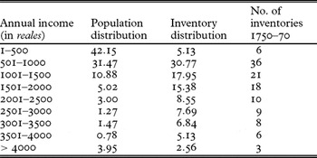
Table 2 summarizes this information: the inventories corresponding to families with annual incomes of 500 reales or less amount to only 4.31 per cent of the total even though 41.15 per cent of the population is in that income range. For family incomes ranging from 501 to 1,000 reales, relative sample size is practically the same as that reflected in the Ensenada Land Registry. Finally, families with annual incomes ranging from 1,001 to 4,000 reales are overrepresented in our sample.
Distribution of population and probate inventories according to annual income as collected in the ‘Ensenada Land Registry’, Palencia (1749–1753)

Source: Ramos (Reference Ramos Palencia2001).
The values in Table 2 were used in the econometric analysis to weight our data set. Thus, each income group is assigned a weight that is equivalent to its share in the total population.Footnote 29
It could be argued that it is risky to attach such a large weight to the poorest group, especially since (i) the size of this group is rather small (it consists of only five observations, and only two of the inventories include any money) and (ii) this group might be atypical in its access to and use of financial assets. Nonetheless, this group seems to exhibit no intrinsically different behavior (in terms of money holding) than the rest of the population: 40 per cent of their inventories include a positive amount of cash, a percentage that is only slightly more than the data set's overall average. Furthermore, although the percentage of net wealth held as cash in this group is the smallest in the data set (0.69 per cent), it is not much below that in other three groups, including the one with incomes between 501 and 1,000 reales (which is the largest group, with 36 observations).Footnote 30 In the first part of the Appendix we present and discuss estimations without weighting; most of the results remain similar to those obtained with the weighted regressions.
The second problem with using probate inventories as a historical source is the risk that cash money may not be registered in the inventory because some heirs (most likely those living in the deceased's household) conceal or steal money before the inventory is taken. On the one hand, inventories were made under the control of official authorities, and heirs − being naturally inclined to protect their own individual interests − serve as a check in this regard; after all, an heir who believes that money has been stolen or an item concealed will have incentive to complain and seek redress.Footnote 31 But on the other hand, some heirs have strong incentives to conceal items prior to the inventory, and money was one of the easiest assets to conceal or steal. We discuss this problem, and present our strategy for dealing with it, in the next section.
5. Estimation and results
The standard approach to estimating money demand assumes that

where Y is a scale variable (usually income or wealth) and i is the interest rate.Footnote 32 The characteristics of our data set make it impossible to include the interest rate in our analysis even though it is a crucial variable in most empirical approaches to money demand. Given that the data set here is based on a cross-section of individuals, the relevant information for our analysis would be the variation in interest rates faced by individuals in the data set. If interest rates are correlated with the dependent variables in our model, then our estimated parameters could be biased.
There is strong reason to believe that richer people face lower interest rates when borrowing because of their reputation and ability to offer collateral. However, the interest rate is relevant when determining the demand for money because it represents the opportunity cost of keeping money in cash. So, the crucial question is whether wealth or other household characteristics (rural versus urban and sector of economy) correlate with interest rates received by lenders (rather than borrowers). It is possible that richer people earn higher interest rates because there are fixed costs associated with accessing the (formal or informal) financial markets; however, there is little clear evidence on this aspect, and research on pre-industrial informal credit market characteristics is rather scarce for Europe (and particularly for Spain).Footnote 33 A more detailed discussion about possible consequences of excluding interest rates in our model is presented in the second part of the Appendix.Footnote 34
The model used in this article to estimate the money demand is

where M is the quantity of money, Y is a measure of wealth, D is a set of dummies providing other information about the characteristics of the household (in our case, D includes the dummy urban and two dummies related to the economic sector, secondary and tertiary), and u is the error term.Footnote 35
There are some advantages of using wealth instead of income when estimating money demand. Given that the endogenous variable (money holdings) is a stock variable, the standard advice of linking stocks with stocks, not stocks with flows, applies. Moreover, some approaches emphasize that money holdings depend more on permanent than on current income and wealth may be a better proxy than current income for permanent income.Footnote 36
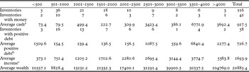
Because we seek to analyse the demand for money, it is important to understand what money was used for in pre-industrial economies and to agree on a definition of money that is relevant for our analysis. It is well known that, in pre-industrial economies, transactions involving basic consumption and day-to-day activities were made with cash but also relied on small debts.Footnote 37 In seventeenth-century England, little money was listed in probate inventories as compared with listed debts; the ratio was 1 to 15 (Muldrew Reference Muldrew1998, p. 100). This suggests a rather sporadic use of money and a more generalized use of debt.Footnote 38 By contrast, in the 116 inventories from Palencia, the average cash holdings were higher than the amounts of money held in debt (917.5 and 726.7 reales, respectively), which suggests a more monetized economy than that of seventeenth-century England.Footnote 39 As it is possible to see in Table 3, on average, the value of money holdings was higher than that of debt instruments across several income groups (according the Catastro de Ensenada), and − except for the poorest − none of the income groups held such ‘positive debts’ worth considerably more than their money held. Money was relatively more abundant in cities than in rural areas: in urban settings, the average cash holding was 1,035 reales while debts averaged 652.6 reales; whereas these quantities were (respectively) 855.7 and 765.7 in the countryside.
Money and positive debt in Probate inventories (in reales)

a Average cash is calculated over all the inventories of the income group (including inventories without cash).
b Average positive debt is calculated over all the inventories of the income group (including inventories without any positive debt).
c Calculated with the information from the Catastro de Ensenada.
Only 39 per cent of the inventories are explicit about the transaction originating the debt. Analysing only those debts for which such details were available reveals that 42 per cent of them are related to labour payments (and these are clearly more abundant in inventories from rural dwellers); 25 per cent of debts were related to the purchase of consumption goods; and 17 per cent were related to payments of rents. The average household had 6.4 of these positive debts in its inventory, and the average value of a debt was quite large: 113 reales.Footnote 40
Given that the use of debt was quite common among all the social classes and that some daily transactions were cancelled with debts instead of money, it would be reasonable to consider debts and money as substitutes. However, when estimating money demand we prefer to use a more restricted definition of money because (i) most of the debts involved relatively large transactions and (ii) there is no evidence, either in the probate inventories or other sources, that the debts were liquid enough to be easily negotiable with third parties. The main results in what follows are not affected if the sum of money and positive debt is used as a proxy for money in our econometric strategy.Footnote 41
Before estimating equation (1) we must decide how to deal with the risk of concealment, as mentioned in Section 4. In our data set only 31 per cent of probate inventories mention cash among belongings, and some inventories of rich individuals include no cash at all, suggesting that a careful analysis of this problem is appropriate.
The very nature of concealment makes it difficult to formulate hypotheses about its characteristics. It is possible for some heirs, in agreement with the rest of the family, to conceal all the money before the inventory is taken; it is also possible that an heir could steal some money yet deliberately leave some just to lend credibility to the final inventory. The possibilities are infinite. To make the issue tractable, we assume that all inventories listing no money are affected by concealment and that all those listing any amount of money are not. Hence the cases without listed money can be regarded as ‘missing observations’ in that we have accurate information about all items in the inventory with the sole exception of money.Footnote 42 Inventories that mention any positive amount of money are assumed to inform accurately about the money holdings (and about all other goods) of the deceased person.
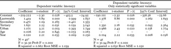
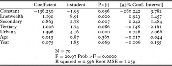
In our application, a simple strategy for econometric analysis is to assume there is no systematic relationship between concealment and other analytical variables, which means we need not model a missing data mechanism for the estimation process. In this case, the simplest procedure is listwise deletion, which removes any observation with missing data from the sample and applies conventional analytical methods to the remaining observations in the data set (Allison Reference Allison2002). Under this assumption, we ran an ordinary least squares (OLS) regression of equation (1) using the 41 observations with positive money holdings. The results are presented in Table 4. The first part of the table presents the output of a regression of the log of money holdings on the log of net wealth, on a dummy for urban dwelling, and on dummies for economic sectors, the age of the deceased person and a time trend. The second part of the table presents the results when the non-significant variables (secondary and age) are excluded from the first regression.
OLS estimation of money demand

*Only 40 observations are included in the regression because one observation does not include the age of the deceased person.
However, suppose concealment is not randomly distributed − for instance, suppose poorer households or rural households tended to conceal more frequently than richer or urban ones. Then bias could arise in our estimates.
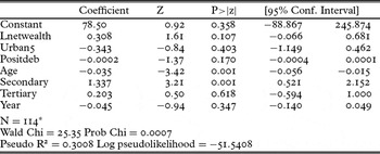
We explore this possibility by first checking whether information in our data set is useful for predicting potential concealment. We estimated a probit model that incorporates a dependent dummy variable of value 1 if some money is included in the inventory (and of value 0 otherwise) as well as all independent variables that could be related to incentives or possibilities for concealing money. See Table 5.
Probit estimation of money demand Dependent variable: du_money

*Only 114 observations are included in the regression because two observations do not include the age of the deceased person.
The only significant variables (at 5 per cent) in this estimation are age (with negative effect) and secondary (with positive effect). This result suggests that, although variables affecting the probability of concealing cash are not the most relevant for estimating money demand, we cannot reject the possibility of a nonrandom sample selection.
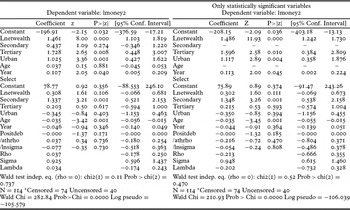
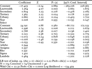
The usual strategy for solving problems of nonrandom sample selection is to apply the Heckman selection model,Footnote 43 for which we need to define, together with the usual regression equation (money demand M = α + βY + γD + u), what is known as the selection equation. This equation states that concealment (m = 0) depends on other variables in the data set. The results of the Heckman estimation are given in Table 6: the first part shows the output of the regression and the selection equations when all possibly relevant variables are included; the second part shows the results when only the statistically significant variables are included in the regression equation.
Heckman estimations of money demand

*Only 114 observations are included in the regression because two observations do not include the age of the deceased person.
There is a strong similarity between the estimated parameters in Table 4 and Table 6. This, together with results of the Wald tests of independent equations in Table 6, suggests that the hypothesis of random distribution of missing observations in our data set is a plausible one.
In what follows we present the quantitative implications of the econometric results obtained using OLS and the Heckman model. Our data set allows us to suggest hypotheses about the relationship between money holdings and characteristics of the deceased person's household such as wealth, type of occupation and place of residence. Because the data set is rather small, we present our results with caution. However, the main risk of a small sample is the possibility of large standard errors and the greater difficulty of rejecting a null hypothesis of parameters being equal to a certain value. Given that our claims are based on those cases in which rejection of the null is possible, we believe that further research with larger data sets will tend to confirm our findings.
One important contribution of this article's methodology is the possibility of estimating the elasticity of money holdings with respect to wealth. Estimates of this elasticity are 1.42 and 1.38 when OLS is used (see Table 4) and 1.46 and 1.49 when the Heckman model is used (Table 6). Confidence intervals in both estimations reveal that we can reject (at the 5 per cent confidence level) not only the null hypothesis of zero elasticity but also the null of unitary elasticity. The only exception is the first equation in the OLS approach, where the lower value of the confidence interval is less than (but still close to) unity.Footnote 44
Because ours is the first money-demand estimation for any period before the nineteenth century, our results can only be compared with empirical analyses of the (second half of the) nineteenth century and the twentieth century. Most of these estimates suggest an income elasticity of demand near 1, but they are based on time-series data and use income as a control variable. Our results are actually quite close to other estimates that use either (i) cross-section data but income as scale variable (with income elasticity between 1.3 and 1.4) or (ii) time-series data and wealth as a scale variable (with a wealth elasticity of 1.32).Footnote 45 This comparison reinforces the plausibility of our results and suggests that the methodological innovation proposed here will prove to be a useful tool for understanding the demand for money.Footnote 46
Our results could yield significant implications if generalized to other pre-industrial economies. Explanations for the evolution of prices, such as the Price Revolution of the sixteenth century, should consider that the demand for money holdings increases more rapidly than wealth and thus, ceteris paribus, that price dampening caused by economic growth is probably more pronounced than suggested by Fisher's equation.Footnote 47
Other estimated parameters in our econometric model facilitate discussion of the nature of the determinants of money holdings with wealth held constant; in the context of the Fisher identity, this would be an indirect way to analyse some determinants of the velocity of circulation. There is no statistically significant relation between the age of a deceased person and money holdings at the time of death.Footnote 48 The time trend is significantly positive and suggests that, all else held equal, cash holdings tend to increase about 10 per cent per year during the period of analysis. With regard to the economic sector, we have included in our model two dummies, tertiary and secondary, that reflect the difference between money holdings of households whose head worked in that sector as compared to households whose head worked in the primary sector (our control group). The implied elasticity of these estimates suggests that people working in the tertiary sector held between 278 per cent and 462 per cent more money than people working in the primary sector.Footnote 49 Estimated parameters for the secondary sector are not significant, indicating that people in primary and secondary sectors had broadly similar money holdings. A rather large tertiary effect is expected, given the money-intensive nature of the tertiary sector, in particular some merchants and small traders whose professional activity required the daily use of rather large quantities of cash.
Our estimates also shed some light on the effect of urbanization. There has been lively debate about whether urbanization implied smaller money holdings (because of more efficient and rapid exchanges) or larger money holdings (because more exchanges imply greater incentive to hold money).Footnote 50 Both econometric models suggest that urbanization leads to an increase in the demand for money: people in cities could have between 162 and 205 per cent more money than those in the countryside.Footnote 51 If our results can be generalized to other areas and periods in pre-industrial Europe, they could offer strong evidence against Goldstone's hypothesis that urbanization pushed price levels up. Indeed, our results show that urbanization increased money demand, suggesting that money became more valuable in terms of goods and that goods became less valuable in terms of money. This dynamic implies declining prices, not rising prices.
6. Conclusions
The main contribution of this article is methodological. We show that it is possible to estimate money demand for pre-industrial economies by using probate inventories, a source available for many places and periods throughout modern Europe. Information provided by probate inventories, although far from perfect, allows a significant advance in understanding the determinants of money demand and the relationships between money holdings and wealth, urbanization and an economy's structure.
With regard to the effect of wealth on money demand, we provide evidence that wealth elasticity is about 1.4 (significantly larger than 1). This implies that economic growth and increased wealth would have produced, ceteris paribus, a larger negative effect on prices than hitherto considered. The estimated effect of urbanization on money holdings is positive, which implies an increase in demand for money and therefore reduced price levels. This initial quantitative evidence regarding the impact of urbanization on the evolution of prices suggests that Goldstone's hypothesis − that a more predominantly urban population increased velocity and thus increased prices − is incorrect. Analysis of the effects of structural change indicates that the tertiary sector is extremely money-intensive, and those in the secondary sector do not hold higher money balances than others in agricultural occupations.
Given that our main contribution is methodological, there is ample room for further research. Two obvious priorities are (i) enlarging the data set and (ii) comparing eighteenth-century Spanish data with data from other periods and other countries. If the use of probate inventories for analysing money demand proves to be the sound idea that we advocate, then a new research area may yield new insights into the monetary history of modern Europe and elsewhere.
Acknowledgements
We wish to thank Dennis Flynn, Lina Gálvez, Jaime Reis, Giovanni Vecchi, Joachim Voth and Eugene White for helpful comments. This article has also benefited from discussions at the Universidad Carlos III de Madrid, Universidad de Tucumán, Universidad de Zaragoza, Universidad de la República (Montevideo), Sciences Po, Universidad Pablo de Olavide, the 5th International Cliometrics in Venice, and the II Iberian Cliometrics Workshop (Iberometrics) in Sigüenza. All remaining errors and omissions are the authors’ responsibility. Esteban Nicolini gratefully acknowledges financial support by the Spanish Ministry of Education and Sciences through Project Consolider-Ingenio 2010, ‘Consolidating Economics’, and through Research Grant ECO2008-02089.
Appendices
1. Results without weighting
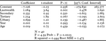
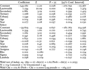
Given the rather small size of the data set and the caveats associated with the weighting strategy, Tables A1 and A2 present the results of estimations (OLS and Heckman models) without weighting observations.
OLS estimation of money demand (equivalent to first equation Table 4 but un-weighted) Dependent variable: lmoney2

Heckman estimation of money demand (equivalent to first equation Table 6 but un-weighted) Dependent variable: lmoney2

In both cases, wealth elasticity is smaller than in the weighted regressions, and urbanization is no longer significant at standard levels; in the Heckman model urbanization is significant at 23 per cent. However most of the estimated parameters remain close to the values obtained with the weighted estimations. The change in the size of the wealth elasticity would suggest that wealth elasticity is not constant but declining in income: when the poorer households are given a smaller weight, income elasticity declines because richer groups ‘dominate’. The small size of the sample precludes the possibility to make a more refined analysis of this hypothesis.
2. Impact of the exclusion of interest rates in the econometric model
The complete equation for a money demand is

where I is the interest rate and the other variables are defined as in Section 5.
If people hold money because of the transactions motive (following, for instance, the approaches of Keynes or Baumol−Tobin), the interest rate should affect money demand because the interest rate is the alternative cost of holding money (i.e. not putting financial wealth into an interest-earning asset). In this context, the higher the interest rate, the lower the demand for money (ψ < 0).
If instead of estimating (A.1) we estimate

then u = ψI + ϵ and, as long as exogenous variables (Y and D) are correlated with the error term, estimated parameters would be biased.
One sensible assumption about why different people face different interest rates in equilibrium is that richer people have better access to financial markets because of fixed costs, reputation, and information advantages. If richer people receive higher interest rates when lending, correlation between Y and u would be positive. Imagine that we represent this lack of orthogonality by assuming that I = φ + θY with θ > 0. Then the true equation would be
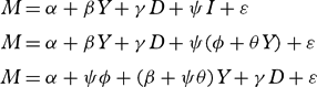
and our estimation of β would be biased. Given that ψθ < 0, our estimation would be biased downwards. However, if sensitivity of money demand to interest rates is low (ψ → 0) or sensitivity of the interest rates to wealth is low (θ → 0), as is probably the case, then bias would be small.
Similar reasoning can be made about possible biases in the estimation of the parameters related to urbanization or economic sector. Probably the most controversial result of our estimation relates to urbanization. If those living in rural settings perceive systematic differences of interest rates vis-à-vis those living in big towns and cities, omission of interest rates in our model would bias our estimation of the impact of urbanization. There is no available evidence supporting the hypothesis of such systematic differences in interest rates; however, common sense suggests higher interest rates for lenders in urban settings because of easier and more flexible access to financial markets. If this is the case, it should be easy to show (following the aforementioned methodology) that the estimation of the parameter related to urbanization is, if anything, biased downward.
3. A broader definition of money
Given the discussion in Section 4, it can be argued that debts and cash were close substitutes and therefore the relevant measure of money holdings should be proxied by the sum of both assets. In Tables A3 and A4 we present the results under this assumption. We have more observations because the set of inventories with positive cash or positive debt is, of course, higher than the set of inventories with positive cash alone. The only change in the qualitative results is associated with the impact of the economic sector: in this setting secondary is positive and statistically significant and tertiary is still positive but its statistical significance drops to 9 per cent. A quantitative change is the higher value of the parameter related to urbanization. The results with the Heckman model are similar to the results with the OLS specification.
OLS estimation of money demand (equivalent to first equation Table 4 but with a broader definition of money) Dependent variable: lm2

Heckman estimation of money demand (equivalent to first equation Table 6 but with a broader definition of money) Dependent variable: lm2