1 Introduction
The dynamical behaviour of plasmas depends markedly on frequencies and scales. At low frequencies and large scales, ions and electrons are locked together and behave like an electrically conducting fluid; this is the regime of magnetohydrodynamics (MHD). At higher frequencies and smaller scales, electrons and ions can move relative to each other, behaving like two separate and interpenetrating fluids: this is the two-fluid regime. However, if the dynamics is supported by non-thermal effects and anisotropies in the velocity space, the more complete kinetic theory is adopted. A notable example is represented by the solar wind, a continuous, highly variable, weakly collisional plasma outflowing at high speed from the Sun. This complex medium is highly structured, with turbulent fluctuations on a wide range of scales, from fractions of a second to several hours, thus covering all the above dynamical ranges.
Spacecraft measurements have revealed that the solar-wind plasma is usually in a state of fully developed turbulence (Marsch Reference Marsch2006; Alexandrova et al. Reference Alexandrova, Chen, Sorriso-Valvo, Horbury and Bale2013; Bruno & Carbone Reference Bruno and Carbone2013). As the turbulent fluctuations expand away from the Sun, these decay and transfer energy to smaller scales. At scales comparable with the ion gyro-radius or the ion inertial length, the MHD approximation fails and kinetic processes involving field–particle interactions take place, along with important cross-scale coupling (Schwartz et al. Reference Schwartz, Hellinger, Bale, Owen, Nakamura, Vaivads, Sorriso-Valvo, Liu, Wimmer-Schweingruber and Fujimoto2011). Furthermore, since the plasma collisionality is quite low, the ion and electron velocity distribution functions (VDFs) can exhibit significant non-Maxwellian signatures. Kinetic processes manifest through the excitation of plasma waves, temperature anisotropy, plasma heating, particle energization, entropy cascade and so on (Vaivads et al. Reference Vaivads, Retinó, Soucek, Khotyaintsev, Valentini and Escoubet2016). Recently, a phenomenological description in terms of cascade in the velocity space, due to highly structured particle distributions, has been proposed (Schekochihin et al. Reference Schekochihin, Parker, Highcock, Dellar, Dorland and Hammett2016; Servidio et al. Reference Servidio, Chasapis, Matthaeus, Perrone, Valentini, Parashar, Veltri, Gershman, Russell and Giles2017). Observations based on the high-resolution ion velocity distribution measurements by the magnetospheric multiscale (MMS) mission in the Earth’s turbulent magnetosheath (Servidio et al. Reference Servidio, Chasapis, Matthaeus, Perrone, Valentini, Parashar, Veltri, Gershman, Russell and Giles2017) have recently confirmed such description, opening new pathways to the understanding of plasma turbulence and dissipation in collisionless plasmas. Numerical simulations are even investigating these features (Cerri et al. Reference Cerri, Kunz and Califano2018; Pezzi et al. Reference Pezzi, Servidio, Perrone, Valentini, Sorriso-Valvo, Greco, Matthaeus and Veltri2018). This cascade may efficiently transfer the energy towards smaller velocity scales, thus producing finer structures in the particle velocity distribution function. The presence of such structures may ultimately enable and enhance the effect of collisions in dissipating the energy (Pezzi et al. Reference Pezzi, Valentini, Perrone and Veltri2013, Reference Pezzi, Valentini, Perrone and Veltri2014, Reference Pezzi, Valentini and Veltri2015a ,Reference Pezzi, Valentini and Veltri b , Reference Pezzi, Valentini and Veltri2016; Pezzi Reference Pezzi2017). Numerical simulations represent an indispensable tool for the understanding of plasma nonlinear dynamics. The use of kinetic numerical simulations is crucial, in fact, when kinetic processes occur in turbulent collisionless plasmas (Parashar et al. Reference Parashar, Shay, Cassak and Matthaeus2009; Camporeale & Burgess Reference Camporeale and Burgess2011; Franci et al. Reference Franci, Verdini, Matteini, Landi and Hellinger2015; Servidio et al. Reference Servidio, Valentini, Perrone, Greco, Califano, Matthaeus and Veltri2015; Cerri et al. Reference Cerri, Califano, Jenko, Told and Rincon2016, Reference Cerri, Servidio and Califano2017; Groselj et al. Reference Groselj, Cerri, Navarro, Willmott, Told, Loureiro, Califano and Jenko2017; Franci et al. Reference Franci, Landi, Verdini, Matteini and Hellinger2018). The Eulerian hybrid Vlasov–Maxwell HVM code (Valentini et al. Reference Valentini, Travnicek, Califano, Hellinger and Mangeney2007; Perrone et al. Reference Perrone, Valentini and Veltri2011) can be used to study the dynamics of a turbulent plasma with typical solar-wind conditions, in order to describe the cross-scale coupling between the MHD turbulence and the small-scale kinetic processes (Valentini et al. Reference Valentini, Veltri, Califano and Mangeney2008; Valentini & Veltri Reference Valentini and Veltri2009; Valentini et al. Reference Valentini, Califano and Veltri2010, Reference Valentini, Califano, Perrone, Pegoraro and Veltri2011a ,Reference Valentini, Perrone and Veltri b ; Perrone et al. Reference Perrone, Valentini and Veltri2011; Greco et al. Reference Greco, Valentini, Servidio and Matthaeus2012; Servidio et al. Reference Servidio, Valentini, Califano and Veltri2012; Perrone et al. Reference Perrone, Valentini, Servidio, Dalena and Veltri2013; Servidio et al. Reference Servidio, Osman, Valentini, Perrone, Califano, Chapman, Matthaeus and Veltri2014; Perrone et al. Reference Perrone, Bourouaine, Valentini, Marsch and Veltri2014a ,Reference Perrone, Valentini, Servidio, Dalena and Veltri b ; Valentini et al. Reference Valentini, Servidio, Perrone, Califano, Matthaeus and Veltri2014; Servidio et al. Reference Servidio, Valentini, Perrone, Greco, Califano, Matthaeus and Veltri2015; Valentini et al. Reference Valentini, Perrone, Stabile, Pezzi, Servidio, De Marco, Marcucci, Bruno, Lavraud and De Keyser2016; Pezzi et al. Reference Pezzi, Malara, Servidio, Valentini, Parashar, Matthaeus and Veltri2017a ,Reference Pezzi, Parashar, Servidio, Valentini, Vásconez, Yang, Malara, Matthaeus and Veltri c ).
For numerical simulations of kinetic turbulence that also include an extended fluid range, the energy level of the small-scale fluctuations may be too low to be investigated with Lagrangian algorithms, unless a large number of particles per cell is used (Franci et al. Reference Franci, Verdini, Matteini, Landi and Hellinger2015). For a convergence study in particle-in-cell (PIC) codes see Haggerty et al. (Reference Haggerty, Parashar, Matthaeus, Shay, Yang, Wan, Wu and Servidio2017). Eulerian-based numerical algorithms might be more suitable for this scope. HVM simulations show that kinetic effects produce, close to reconnection regions, a distortion of the ion velocity distribution, through the generation of accelerated field-aligned beams, temperature anisotropy and trapped particle populations. Moreover, although the addition of heavy ions does not considerably affect the inertial-range turbulent cascade (Perrone et al. Reference Perrone, Valentini, Servidio, Dalena and Veltri2013), departures from the Maxwellian shape are more pronounced for heavy ions than for protons (Perrone et al. Reference Perrone, Valentini, Servidio, Dalena and Veltri2013, Reference Perrone, Valentini, Servidio, Dalena and Veltri2014b ; Valentini et al. Reference Valentini, Perrone, Stabile, Pezzi, Servidio, De Marco, Marcucci, Bruno, Lavraud and De Keyser2016), pointing out that the role of secondary ions must be considered for understanding energy partition in plasmas (Marsch Reference Marsch2006; Kasper et al. Reference Kasper, Lazarus and Gary2008; Araneda et al. Reference Araneda, Maneva and Marsch2009; Maneva et al. Reference Maneva, Vinas, Moya, Wicks and Poedts2015). Although the physical mechanisms of solar-wind turbulence have been a matter of investigation for many decades, both using in situ measurements and numerical experiments, important problems concerning the interconnection between the inertial and kinetic-range processes, as well as the interplay between physical space fluctuations and velocity space perturbations, are still poorly understood.
Solar-wind turbulence is characterized by intermittency (Burlaga Reference Burlaga1991; Frisch Reference Frisch1995), i.e. the spatial inhomogeneity of the energy transfer across scales, that results in the generation of highly energetic, bursty small-scale fluctuations with scale-dependent, non-Gaussian statistics (Sorriso-Valvo et al. Reference Sorriso-Valvo, Carbone, Veltri, Consolini and Bruno1999). Such fluctuations are often referred to as coherent structures, with phase synchronization among a certain number of scales (Greco & Perri Reference Greco and Perri2014; Lion et al. Reference Lion, Alexandrova and Zaslavsky2016; Perrone et al. Reference Perrone, Alexandrova, Mangeney, Maksimovic, Lacombe, Rakoto, Kasper and Jovanovic2016, Reference Perrone, Alexandrova, Roberts, Lion, Lacombe, Walsh, Maksimovic and Zouganelis2017; Roberts et al. Reference Roberts, Li, Alexandrova and Li2016). At smaller scales, below the MHD range, a more variable level of intermittency is observed, whose nature is still under debate (Alexandrova et al. Reference Alexandrova, Carbone, Veltri and Sorriso-Valvo2008; Kiyani et al. Reference Kiyani, Chapman, Khotyaintsev, Dunlop and Sahraoui2009). In recent years, the study of the intermittency and the consequent research on small-scale structures have been performed by using different methods. For example, wavelet analysis (Farge Reference Farge1992; Bruno et al. Reference Bruno, Bavassano, Pietropaolo, Carbone and Veltri1999) provides the local estimation of the scale-dependent energy associated with the magnetic fluctuations, thus allowing the identification of the highly energetic intermittent structures. Alternatively, the partial variance of increments (PVI) technique (Greco et al. Reference Greco, Chuychai, Matthaeus, Servidio and Dimitruk2008) was used to identify discontinuities, current sheets and other intermittent features.
Recently, there is a compelling evidence that the kinetic processes are enhanced in the proximity of the turbulence-generated structures, which carry a larger amount of energy than the turbulent background. Measurements have shown that both ions and electrons are energized in the proximity of the most intense small-scale current sheets (Osman et al. Reference Osman, Matthaeus, Greco and Servidio2011, Reference Osman, Matthaeus, Hnat and Chapman2012; Tessein et al. Reference Tessein, Matthaeus, Wan, Osman, Ruffolo and Giacalone2013; Chasapis et al. Reference Chasapis, Retinò, Sahraoui, Vaivads, Khotyaintsev, Sundkvist, Greco, Sorriso-Valvo and Canu2015, Reference Chasapis, Matthaeus, Parashar, LeContel, Retinò, Breuillard, Khotyaintsev, Vaivads, Lavraud and Eriksson2017). Note that the same behaviour has been observed in HVM numerical simulations (Greco et al. Reference Greco, Valentini, Servidio and Matthaeus2012; Servidio et al. Reference Servidio, Valentini, Califano and Veltri2012; Perrone et al. Reference Perrone, Valentini, Servidio, Dalena and Veltri2014b ). More recently, even reduced models such as gyro-kinetics converged toward this general view (Howes Reference Howes2016; Howes et al. Reference Howes, McCubbin and Klein2018). The processes responsible for such different forms of energization may involve magnetic reconnection (Retinò et al. Reference Retinò, Sundkvist, Vaivads, Mozer, André and Owen2007; Burch et al. Reference Burch, Torbert, Phan, Chen, Moore, Ergun, Eastwood, Gershman, Cassak and Argall2016b ), wave–particle resonances, plasma instabilities (Matteini et al. Reference Matteini, Hellinger, Goldstein, Landi, Velli and Neugebauer2013; Servidio et al. Reference Servidio, Osman, Valentini, Perrone, Califano, Chapman, Matthaeus and Veltri2014; Breuillard et al. Reference Breuillard, Yordanova, Vaivads and Alexandrova2016) and enhancement of collisions (Pezzi et al. Reference Pezzi, Valentini and Veltri2016). These topics are currently debated in the space plasma community (Chen Reference Chen2016).
In order to understand the interconnections between the turbulent structures and the small-scale kinetic processes, a more detailed description of the local energy flux across scales should be defined for plasma turbulence. This possible tool should take into account the complex nature of the nonlinear coupling between the velocity and magnetic field. Recent studies included the contributions from cross-terms, typically associated with Alfvénic fluctuations, to better identify regions of small-scale accumulation of energy (Sorriso-Valvo et al. Reference Sorriso-Valvo, Marino, Lijoi, Perri and Carbone2015).
In MHD, the energy transfer across scales obeys the Politano–Pouquet law (PP) (Politano & Pouquet Reference Politano and Pouquet1998), which prescribes the linear scaling of the mixed third-order moment of the field increments. The proportionality factor is the mean energy transfer rate
 $\langle \unicode[STIX]{x1D716}^{\pm }\rangle$
, the brackets indicating ensemble average. For a two-dimensional field, the standard version of the PP law for the mixed third-order moments
 $Y^{\pm }(l)$
is
 $$\begin{eqnarray}Y^{\pm }(l)=\langle |\unicode[STIX]{x0394}{\boldsymbol{z}^{\pm }}_{l}(\boldsymbol{r})|^{2}\,\unicode[STIX]{x0394}z_{i,l}^{\mp }(\boldsymbol{r})\rangle =-2\langle \unicode[STIX]{x1D716}^{\pm }\rangle l.\end{eqnarray}$$
 $\unicode[STIX]{x0394}\unicode[STIX]{x1D713}_{l}=\unicode[STIX]{x1D713}(\boldsymbol{r}+l\boldsymbol{r}/r)-\unicode[STIX]{x1D713}(\boldsymbol{r})$
is the longitudinal increment of a generic field
 $\unicode[STIX]{x1D713}$
(e.g. the magnetic field
 $\boldsymbol{B}(\boldsymbol{r})$
) across the scale
 $l$
; the subscript
 $i$
indicates the generic component of the field, the field increment being estimated along the same direction;
 $\boldsymbol{z}^{\pm }=\boldsymbol{v}\pm \boldsymbol{B}/\sqrt{4\unicode[STIX]{x03C0}\unicode[STIX]{x1D70C}}$
are the Elsasser variables that couple the plasma velocity
 $\boldsymbol{v}$
and the magnetic field
 $\boldsymbol{B}$
, the latter being expressed in velocity units through the plasma density
 $\unicode[STIX]{x1D70C}$
. The validity of the PP law has been first verified in two-dimensional MHD numerical simulations (Sorriso-Valvo et al.
Reference Sorriso-Valvo, Carbone, Noullez, Politano, Pouquet and Veltri2002), and later also in the solar wind (MacBride et al.
Reference MacBride, Forman, Smith, Fleck, Zurbuchen and Lacoste2005; Sorriso-Valvo et al.
Reference Sorriso-Valvo, Marino, Carbone, Noullez, Lepreti, Veltri, Bruno, Bavassano and Pietropaolo2007; MacBride et al.
Reference MacBride, Smith and Forman2008; Marino et al.
Reference Marino, Sorriso-Valvo, Carbone, Noullez, Bruno and Bavassano2008, Reference Marino, Sorriso-Valvo, D’Amicis, Carbone, Bruno and Veltri2012).
Based on the PP law (1.1), an heuristic proxy of the ‘local’ energy transfer rate (LET) at the scale
 $l$
can be defined by introducing the quantity:
 $$\begin{eqnarray}\unicode[STIX]{x1D716}_{l}(\boldsymbol{r})=-\frac{1}{2l}[|\unicode[STIX]{x0394}\boldsymbol{z}_{l}^{+}(\boldsymbol{r})|^{2}\,\unicode[STIX]{x0394}z_{i,l}^{-}(\boldsymbol{r})+|\unicode[STIX]{x0394}\boldsymbol{z}_{l}^{-}(\boldsymbol{r})|^{2}\,\unicode[STIX]{x0394}z_{i,l}^{+}(\boldsymbol{r})].\end{eqnarray}$$
At a given scale, each field increment in the time series can thus be associated with the local value of
 $\unicode[STIX]{x1D716}_{l}(\boldsymbol{r})$
(Marsch & Tu Reference Marsch and Tu1997; Sorriso-Valvo et al.
Reference Sorriso-Valvo, Marino, Lijoi, Perri and Carbone2015, Reference Sorriso-Valvo, Carbone, Perri, Greco, Marino and Bruno2018). Note that the LET can be expressed in terms of velocity and magnetic field as
 $\unicode[STIX]{x1D716}_{l}(\boldsymbol{r})\propto \unicode[STIX]{x0394}v_{i}(\unicode[STIX]{x0394}v^{2}+\unicode[STIX]{x0394}b^{2})-2\unicode[STIX]{x0394}b_{i}(\unicode[STIX]{x0394}\boldsymbol{v}\boldsymbol{\cdot }\unicode[STIX]{x0394}\boldsymbol{b})$
. The first right-hand side term is associated with the total energy advected by the velocity fluctuations, and is correlated to the total PVI (i.e. including both velocity and magnetic increments). The second term is associated with the velocity–magnetic field correlations coupled to the longitudinal magnetic field fluctuations (Andrés & Sahraoui Reference Andrés and Sahraoui2017; Sorriso-Valvo et al.
Reference Sorriso-Valvo, Carbone, Perri, Greco, Marino and Bruno2018). Recently, by using Helios 2 data, it has been shown that the LET correctly identifies the regions of space in the turbulent solar wind that carry energy towards smaller scales. These regions are characterized by enhanced kinetic processes, resulting in a higher proton temperature (Sorriso-Valvo et al.
Reference Sorriso-Valvo, Carbone, Perri, Greco, Marino and Bruno2018). It is worth noting that in recent works, the third-order law in (1.1) has been extended to include characteristic plasma length scales and compressibility (Andrés et al.
Reference Andrés, Galtier and Sahraoui2018).
The correlation between the local temperature increase and the large amplitude bursts of energy transfer suggests that the proxy defined in (1.2) might play an important role in the understanding of solar-wind turbulent dissipation and heating. Moreover, the comparison between the properties of the PVI and LET has shown that both methods are suitable for the description of the turbulent energy cascade, although the LET carries additional information related to the correlations between velocity magnetic turbulent fluctuations. Additionally, since the LET is a signed variable, in principle it should also carry additional information about the possible direction of the cross-scale energy flow, identifying possible local direct and inverse cascade processes. The latter cannot be studied by using PVI or wavelet-based techniques since these are positive–defined.
The aim of this paper is to explore the link between the MHD turbulent energy cascade and the kinetic processes associated with deviations of the ion velocity distributions from the Maxwellian equilibrium. To this aim, we make use of the LET for interpreting high-resolution data from numerical simulations of the Vlasov–Maxwell multi-component system. The present work is organized as follows. In § 2 the governing equations, the numerical algorithm and the parameters of the Vlasov simulations will be presented. A brief overview on the numerical results will be given. The use of the proxy of the local energy transfer rate will be the topic of § 3, while in § 4 we will discuss our conclusions.
2 HVM multi-component simulations
We use high-resolution Vlasov simulations in order to simulate the turbulent multi-species plasma of the solar wind. First, high spatial resolution is needed in order to follow the evolution of the turbulent cascade up to wavelengths shorter than ion characteristic scales, where kinetic effects presumably govern the physics of the system. Second, high numerical resolution in the velocity domain is required to investigate the distortions of the ion distribution functions. The above two requirements are the main ingredients of the highly performing, extensively tested, HVM code (http://fis.unical.it/hvm/).
2.1 Numerical method
We employ the HVM code which directly integrates the Vlasov equations for both proton and
 $\unicode[STIX]{x1D6FC}$
particle distribution functions while electrons are considered as a massless isothermal fluid. The Vlasov equation for both ion species is combined with the Maxwell system, by assuming quasi-neutrality and by neglecting the displacement current. In particular Ampére and Faraday equations and a generalized Ohm’s law are solved. HVM equations, written in dimensionless form, are the following:
 $$\begin{eqnarray}\displaystyle \frac{\unicode[STIX]{x2202}f_{s}}{\unicode[STIX]{x2202}t}+\boldsymbol{v}\boldsymbol{\cdot }\frac{\unicode[STIX]{x2202}f_{s}}{\unicode[STIX]{x2202}\boldsymbol{r}}+\unicode[STIX]{x1D706}_{s}\left(\boldsymbol{E}+\boldsymbol{v}\times \boldsymbol{B}\right)\boldsymbol{\cdot }\frac{\unicode[STIX]{x2202}f_{s}}{\unicode[STIX]{x2202}\boldsymbol{v}}=0 & & \displaystyle\end{eqnarray}$$
 $$\begin{eqnarray}\displaystyle \boldsymbol{E}=-\left(\boldsymbol{u}_{e}\times \boldsymbol{B}\right)-\frac{\unicode[STIX]{x1D735}P_{e}}{n_{e}}+\unicode[STIX]{x1D702}\boldsymbol{j} & & \displaystyle\end{eqnarray}$$
 $$\begin{eqnarray}\displaystyle \frac{\unicode[STIX]{x2202}\boldsymbol{B}}{\unicode[STIX]{x2202}t}=-\unicode[STIX]{x1D735}\times \boldsymbol{E};\quad \unicode[STIX]{x1D735}\times \boldsymbol{B}=\boldsymbol{j}. & & \displaystyle\end{eqnarray}$$
In the previous equations,
 $f_{s}(\boldsymbol{r},\boldsymbol{v},t)$
is the ion distribution function (the subscript
 $s=p,\unicode[STIX]{x1D6FC}$
refers to protons and
 $\unicode[STIX]{x1D6FC}$
particles, respectively),
 $\boldsymbol{E}(\boldsymbol{r},t)$
and
 $\boldsymbol{B}(\boldsymbol{r},t)$
are the electric and magnetic fields, respectively and
 $\unicode[STIX]{x1D706}_{s}$
is a constant reflecting the charge to mass ratio of each species (
 $\unicode[STIX]{x1D706}_{p}=1$
,
 $\unicode[STIX]{x1D706}_{\unicode[STIX]{x1D6FC}}=1/2$
). The electron bulk speed is
 $\boldsymbol{u}_{e}=(\sum _{s}Z_{s}n_{s}\boldsymbol{u}_{s}-\boldsymbol{j})/n_{e}$
, where
 $Z_{s}$
is the ion charge number (
 $Z_{p}=1$
,
 $Z_{\unicode[STIX]{x1D6FC}}=2$
), the ion density
 $n_{s}$
and the ion bulk velocity
 $\boldsymbol{u}_{s}$
are the zeroth- and first-order moments of the ion distribution function, respectively, and the electron density
 $n_{e}$
is evaluated through the quasi-neutrality condition
 $n_{e}=\sum _{s}Z_{s}n_{s}$
. Furthermore,
 $P_{e}=n_{e}T_{e}$
is the electron pressure (
 $T_{e}$
is homogeneous and stationary) and
 $\boldsymbol{j}=\unicode[STIX]{x1D735}\times \boldsymbol{B}$
is the total current density. The external small resistivity
 $\unicode[STIX]{x1D702}=2\times 10^{-2}$
is introduced to remove spurious numerical instabilities. In (2.1)–(2.3), masses, charges, time, velocities and lengths are respectively normalized to the proton mass,
 $m_{p}$
, and charge,
 $e$
, to the inverse of the proton cyclotron frequency,
 $\unicode[STIX]{x1D6FA}_{cp}^{-1}=m_{p}c/eB_{0}$
(being
 $c$
and
 $B_{0}$
the speed of light and the ambient magnetic field), to the Alfvén velocity,
 $V_{A}=B_{0}/\sqrt{4\unicode[STIX]{x03C0}n_{0,p}m_{p}}$
(being
 $n_{0,p}$
the equilibrium proton density) and to the proton skin depth,
 $d_{p}=V_{A}/\unicode[STIX]{x1D6FA}_{cp}$
.
The described set of (2.1)–(2.3) are solved in a phase space domain with 2.5 spatial and 3 velocity-space dimensions, so that all vector components are retained but they depend only on the two spatial coordinates
 $(x,y)$
. The spatial domain, whose size is
 $L=2\unicode[STIX]{x03C0}\times 20d_{p}$
in both directions, has been discretized with
 $512^{2}$
grid points and, at boundaries, periodic conditions are implemented. Each direction of the velocity domain of each species (protons and
 $\unicode[STIX]{x1D6FC}$
particles) is discretized with
 $71$
grid points in the range
 $v_{j,s}=[-v_{\text{max},s},v_{\text{max},s}]~(j=x,y,z)$
, where
 $v_{\text{max},s}=\pm 5v_{th,s}$
(being
 $v_{th,s}=\sqrt{k_{B}T_{0,s}/m_{s}}$
the ion thermal speed, with
 $T_{0,s}$
the equilibrium temperature). Boundary conditions in velocity space assume
 $f_{s}(|v|>v_{\text{max},s})=0$
in each direction. The time step
 $\unicode[STIX]{x0394}t$
has been chosen in such a way that the Courant–Friedrichs–Lewy (CFL) condition for the numerical stability of the Vlasov algorithm is satisfied (Peyret & Taylor Reference Peyret and Taylor1986). To control the numerical accuracy of the simulation, the basic set of conservation laws of Vlasov equation is continuously monitored during the simulations: relative variation of proton mass,
 $\unicode[STIX]{x1D6FC}$
particle mass, total energy and entropy are approximately
 $2.5\times 10^{-3}\,\%$
,
 $3.5\times 10^{-1}\,\%$
,
 $0.6\,\%$
and
 $0.4\,\%$
, respectively.
At the initial time of the simulation (
 $t=0$
), both ion species have Maxwellian distribution functions, with homogeneous densities, and an uniform background out-of-plane magnetic field
 $\boldsymbol{B}_{\mathbf{0}}=B_{0}\boldsymbol{e}_{z}$
is imposed. In order to mimic the physical conditions of the pristine solar wind, we assume that (i) the
 $\unicode[STIX]{x1D6FC}$
particle to proton density ratio
 $n_{0,\unicode[STIX]{x1D6FC}}/n_{0,p}=5\,\%$
and (ii) we consider
 $\unicode[STIX]{x1D6FC}$
particles, protons and electrons at the same initial temperature
 $T_{0,\unicode[STIX]{x1D6FC}}=T_{0,p}=T_{e}$
. The equilibrium is then perturbed through a 2-D spectrum of Fourier modes in the plane
 $(x,y)$
, for both proton bulk velocity and magnetic field, such that proton bulk velocity and magnetic field are globally uncorrelated. Energy is injected with wavenumbers in the range
 $0.1<k<0.3$
(
 $2\leqslant m\leqslant 6$
, where
 $k=2\unicode[STIX]{x03C0}m/L$
) and random phases. We did not introduce neither density disturbances nor parallel variances, i.e.
 $\unicode[STIX]{x1D6FF}n=\unicode[STIX]{x1D6FF}u_{z}=\unicode[STIX]{x1D6FF}B_{z}=0$
at
 $t=0$
. The root-mean-square (r.m.s.) level of fluctuations is
 $\unicode[STIX]{x1D6FF}B/B_{0}=1/3$
, while
 $\unicode[STIX]{x1D6FD}_{p}=2v_{th,p}^{2}/V_{A}^{2}=0.5$
.
The kinetic evolution of protons and
 $\unicode[STIX]{x1D6FC}$
particles is numerically investigated in a decaying turbulence. During the simulation, nonlinear couplings between fluctuations generate a turbulent cascade, where the injected energy is transferred along the spectrum to smaller, kinetic scales. The time
 $t^{\ast }$
of maximum turbulent activity can be identified as the peak time of the spatially averaged out-of-plane current density,
 $\langle \,j_{z}^{2}\rangle$
, a standard indicator for small-scale magnetic gradients. All the analysis has been performed using one snapshot of the simulation at
 $t^{\ast }\unicode[STIX]{x1D6FA}_{cp}=49$
, when decaying turbulence approaches a quasi-steady state. A more detailed description of the numerical results of the simulation can be found in Valentini et al. (Reference Valentini, Perrone, Stabile, Pezzi, Servidio, De Marco, Marcucci, Bruno, Lavraud and De Keyser2016).
2.2 Numerical results
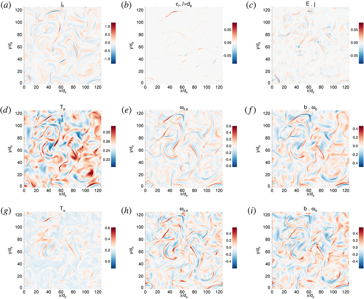
An overview of the differential kinetic dynamics of the ion species, namely protons and
 $\unicode[STIX]{x1D6FC}$
particles, associated with the development of the turbulent cascade, is presented in figure 1. Turbulence leads to the generation of small-scale coherent structures, such as current sheets, filaments or strongly shared flows, which can be recognized in the two-dimensional patterns in physical space. In particular, figure 1(a) shows the shaded contours of the out-of-plane current density,
 $j_{z}$
. The current density becomes very intense in between magnetic islands, where magnetic reconnection can locally occur.
Two-dimensional contour plots for the HVM multi-component simulation at
 $t=t^{\ast }$
. (a) The out-of-plane total current density
 $j_{z}$
; (b) the local energy transfer rate
 $\unicode[STIX]{x1D716}_{d_{p}}$
; (c)
 $\boldsymbol{E}\boldsymbol{\cdot }\boldsymbol{j}$
; (d) the proton temperature
 $T_{p}$
; (e) the out-of-plane proton vorticity
 $\unicode[STIX]{x1D714}_{z,p}$
; (f)
 $\boldsymbol{b}\boldsymbol{\cdot }\unicode[STIX]{x1D714}_{p}$
; (g) the
 $\unicode[STIX]{x1D6FC}$
particle temperature
 $T_{\unicode[STIX]{x1D6FC}}$
; (h) the out-of-plane
 $\unicode[STIX]{x1D6FC}$
particle vorticity
 $\unicode[STIX]{x1D714}_{z,\unicode[STIX]{x1D6FC}}$
; and (i)
 $\boldsymbol{b}\boldsymbol{\cdot }\unicode[STIX]{x1D714}_{\unicode[STIX]{x1D6FC}}$
.

Figure 1(b) shows the contour map of the local energy transfer rate,
 $\unicode[STIX]{x1D716}_{l}(x,y)$
, estimated using the velocity and magnetic field (in Alfvén units) two-point increments at the scale
 $l=d_{p}$
. Positive and negative filaments of strong energy transfer
 $\unicode[STIX]{x1D716}_{l}$
are present, but the spatial correlation with strong current sheets is unclear. There is a shift between the current layers and this cascade-transfer indicator, probably due to the fact that the former are the sites of dissipation, while the LET is high at the very active nonlinear regions, such as the upstream parts of the reconnecting current sheets.
In figure 1(c) we display the contour map of
 $\boldsymbol{E}\boldsymbol{\cdot }\boldsymbol{j}$
, a proxy of energy conversion between fields and particles (Wan et al.
Reference Wan, Matthaeus, Roytershteyn, Karimabadi, Parashar, Wu and Shay2015; Yang et al.
Reference Yang, Matthaeus, Parashar, Wu, Wan, Shi, Chen, Roytershteyn and Daughton2017). Large positive values are observed in the proximity of the strongest current sheets, suggesting that the electromagnetic energy might be converted into kinetic and thermal energy where magnetic reconnection is likely to occur.
Figure 1(d,g) show the maps of proton and
 $\unicode[STIX]{x1D6FC}$
-particle temperature, respectively, defined as the second-order velocity moment of the ion distribution function. Comparison with panel (a) highlights that the presence of strong current sheets corresponds to temperature enhancement of both ions. Although the initial conditions of the simulation infer equal and uniform temperature for the two ion species, during the turbulent evolution of the system both ions show a non-uniform temperature pattern, with similar inhomogeneity as for the current
 $j_{z}$
. Colour bars were chosen so that the initial temperature
 $T_{0}$
is white, while red and blue indicate local heating and cooling, respectively. A definite temperature increase can be observed close to the region of strong magnetic field gradients, meaning that the heating processes are influenced by the topology of the magnetic field. Preferential heating is also evident, as the
 $\unicode[STIX]{x1D6FC}$
particles temperature is nearly twice that of the protons. Moreover, while the protons display roughly equal heating and cooling with respect to the initial temperature
 $T_{0}$
, the
 $\unicode[STIX]{x1D6FC}$
particles show predominant temperature increase.
Enhanced ion heating was recently observed in spatial regions nearby the peaks of the ion vorticity
 $\unicode[STIX]{x1D714}=\unicode[STIX]{x1D735}\times \boldsymbol{v}$
(Servidio et al.
Reference Servidio, Valentini, Perrone, Greco, Califano, Matthaeus and Veltri2015; Franci et al.
Reference Franci, Hellinger, Matteini, Verdini, Landi and Wang2016; Valentini et al.
Reference Valentini, Perrone, Stabile, Pezzi, Servidio, De Marco, Marcucci, Bruno, Lavraud and De Keyser2016). Previous studies have shown the association between viscous-like effects, velocity shears (Markovskii et al.
Reference Markovskii, Vasquez, Smith and Hollweg2006; Del Sarto et al.
Reference Del Sarto, Pegoraro and Califano2016) and vorticity (Huba Reference Huba1996), including the dependence on the sign of
 $\boldsymbol{B}_{0}\boldsymbol{\cdot }\unicode[STIX]{x1D74E}$
(Parashar & Matthaeus Reference Parashar and Matthaeus2016). In particular, it has been shown that the vorticity may enhance local kinetic effects, with a generalized resonance sign-dependence condition for the enhancement or reduction of the ion heating and temperature anisotropy (Parashar & Matthaeus Reference Parashar and Matthaeus2016). In order to explore such correlation, the maps of the out-of-plane ion vorticities
 $\unicode[STIX]{x1D714}_{z,p}$
and
 $\unicode[STIX]{x1D714}_{z,\unicode[STIX]{x1D6FC}}$
, are shown in figure 1(e,h). A pattern of small-scale vorticity structures can be observed, similar to the case of the current. However, a more complex topology is observed for the
 $\unicode[STIX]{x1D6FC}$
particles vorticity, with the splitting of the structures in smaller filaments already observed in Hall-MHD turbulence (Martin Reference Martin, De Vita, Sorriso-Valvo, Dimitruck, Nigro, Primavera and Carbone2013).
Finally, in figure 1(f,i) we show the 2-D contour plot of
 $\boldsymbol{b}\boldsymbol{\cdot }\unicode[STIX]{x1D74E}$
for both protons and
 $\unicode[STIX]{x1D6FC}$
particles, respectively, where
 $\boldsymbol{b}=\boldsymbol{B}-\boldsymbol{B}_{\mathbf{0}}$
indicates the magnetic field fluctuations. A behaviour similar to
 $\unicode[STIX]{x1D714}_{z}$
is observed, so that both positive
 $\unicode[STIX]{x1D714}_{z}$
and
 $\boldsymbol{b}\boldsymbol{\cdot }\unicode[STIX]{x1D74E}$
correspond to increased temperature, for both ion species.
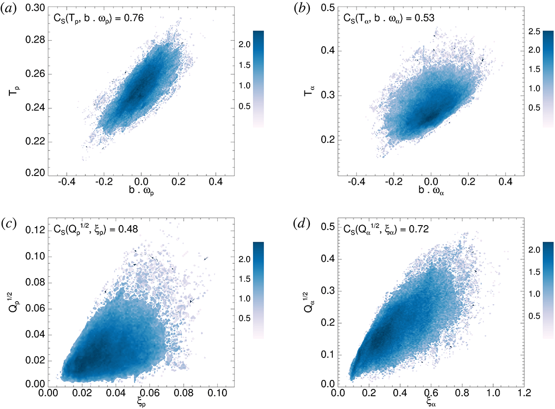
Joint probability distributions for (a)
 $T_{p}$
and
 $\boldsymbol{b}\boldsymbol{\cdot }\unicode[STIX]{x1D74E}_{p}$
; (b)
 $T_{\unicode[STIX]{x1D6FC}}$
and
 $\boldsymbol{b}\boldsymbol{\cdot }\unicode[STIX]{x1D74E}_{\unicode[STIX]{x1D6FC}}$
; (c)
 $Q_{p}^{1/2}$
and
 $\unicode[STIX]{x1D709}_{p}$
; (d)
 $Q_{\unicode[STIX]{x1D6FC}}^{1/2}$
and
 $\unicode[STIX]{x1D709}_{\unicode[STIX]{x1D6FC}}$
.

The overview of the numerical results of the HVM multi-species simulation given in figure 1 highlights a general enhancement of the ion temperature related to the presence of thin current sheets. A more evident correlation is found with the ion out-of-plane vorticity
 $\unicode[STIX]{x1D714}_{s}$
and with
 $\boldsymbol{b}\boldsymbol{\cdot }\unicode[STIX]{x1D714}_{s}$
. To better appreciate the robustness of the observed correlation between
 $T_{s}$
and
 $\boldsymbol{b}\boldsymbol{\cdot }\unicode[STIX]{x1D74E}_{s}$
, in figure 2(a,b) of we show the average joint probability distributions
 $P(T_{p},\boldsymbol{b}\boldsymbol{\cdot }\unicode[STIX]{x1D74E}_{p})$
and
 $P(T_{\unicode[STIX]{x1D6FC}},\boldsymbol{b}\boldsymbol{\cdot }\unicode[STIX]{x1D74E}_{\unicode[STIX]{x1D6FC}})$
, respectively. A good correlation is observed for both ion species, that we quantify through the nonlinear Spearman correlation coefficients,
 $C_{S}$
, indicated in each panel of figure 2. Correlations are stronger for protons
 $[C_{S}(T_{p},\boldsymbol{b}\boldsymbol{\cdot }\unicode[STIX]{x1D74E}_{p})=0.76]$
, than for
 $\unicode[STIX]{x1D6FC}$
particles
 $[C_{S}(T_{\unicode[STIX]{x1D6FC}},\boldsymbol{b}\boldsymbol{\cdot }\unicode[STIX]{x1D74E}_{\unicode[STIX]{x1D6FC}})=0.53]$
. However, the correlation between the temperature and the out-of-plane vorticity (i.e. the vorticity component parallel to the background magnetic field rather than to the magnetic fluctuations) is larger for the
 $\unicode[STIX]{x1D6FC}$
particles:
 $C_{S}(T_{p},\unicode[STIX]{x1D714}_{z,p})=0.49$
and
 $C_{S}(T_{\unicode[STIX]{x1D6FC}},\unicode[STIX]{x1D714}_{z,\unicode[STIX]{x1D6FC}})=0.63$
(joint distributions are not shown for this case). The heating is thus better correlated with the out-of-plane vorticity for the
 $\unicode[STIX]{x1D6FC}$
particles, but with the vorticity component parallel to the local magnetic fluctuations for the protons. This may be related to the heavier
 $\unicode[STIX]{x1D6FC}$
particles being slower than protons in following the magnetic field fluctuations.
The heating mechanisms are also correlated with strong deformation of the ion velocity distribution (Servidio et al. Reference Servidio, Valentini, Califano and Veltri2012; Valentini et al. Reference Valentini, Perrone, Stabile, Pezzi, Servidio, De Marco, Marcucci, Bruno, Lavraud and De Keyser2016). For each ion species and in each point of the simulation domain, the non-Maxwellian measure can be defined as (Greco et al. Reference Greco, Valentini, Servidio and Matthaeus2012; Vasconez et al. Reference Vasconez, Pucci, Valentini, Servidio, Matthaeus and Malara2015; Pucci et al. Reference Pucci, Vasconez, Pezzi, Servidio, Valentini, Matthaeus and Malara2016; Pezzi et al. Reference Pezzi, Parashar, Servidio, Valentini, Vásconez, Yang, Malara, Matthaeus and Veltri2017b ; Valentini et al. Reference Valentini, Vasconez, Pezzi, Servidio, Malara and Pucci2017):
 $$\begin{eqnarray}\displaystyle \unicode[STIX]{x1D709}_{s}=\frac{1}{n_{s}}\sqrt{\int \!(f_{s}-g_{s})^{2}\,\text{d}^{3}v}. & & \displaystyle\end{eqnarray}$$
The above scalar function measures the deviation of the observed distribution
 $f_{s}$
from the associated Maxwellian
 $g_{s}$
, which is built using the local density, bulk velocity and temperature. The latter quantity is also intimately related to the so-called velocity space cascade, recently observed in space plasmas (Servidio et al.
Reference Servidio, Chasapis, Matthaeus, Perrone, Valentini, Parashar, Veltri, Gershman, Russell and Giles2017).
It is useful at this point to consider the agyrotropy of the pressure tensor, i.e. its departure from cylindrical symmetry around the local magnetic field direction. Non-gyrotropy is important as a known source of instabilities, and may help identifying spatial structures in the plasma (Scudder & Daughton Reference Scudder and Daughton2008; Aunai et al.
Reference Aunai, Hesse and Kuznetsova2013; Swisdak Reference Swisdak2016). For both ion species, given the
 $3\times 3$
pressure tensor with elements
 $\unicode[STIX]{x1D617}_{ij}$
in an arbitrary Cartesian system with coordinates
 $(x,y,z)$
, the measure of agyrotropy can be defined as the scalar (Swisdak Reference Swisdak2016):
 $$\begin{eqnarray}\displaystyle \unicode[STIX]{x1D618}_{s}=1-\frac{4I_{2,s}}{(I_{1,s}-P_{\Vert ,s})(I_{1,s}+3P_{\Vert ,s})}, & & \displaystyle\end{eqnarray}$$
with
 $I_{1}=P_{xx}+P_{yy}+P_{zz}$
, and
 $I_{2}=P_{xx}P_{yy}+P_{xx}P_{zz}+P_{yy}P_{zz}-(P_{xy}P_{yx}+P_{xz}P_{zx}+P_{yz}P_{zy})$
.
 $P_{\Vert }$
here represents the parallel pressure, where we have omitted the subscript
 $s$
for simplicity. A good correlation is observed between the non-gyrotropy of the ion pressure tensor,
 $\unicode[STIX]{x1D618}_{s}^{1/2}$
, and the non-Maxwellianity of the ion velocity,
 $\unicode[STIX]{x1D709}_{s}$
, as shown in the joint probability distribution maps in of figure 2(c,d) for protons and
 $\unicode[STIX]{x1D6FC}$
particles, respectively. This mechanism works better for
 $\unicode[STIX]{x1D6FC}$
particles
 $[C_{S}(Q_{\unicode[STIX]{x1D6FC}}^{1/2},\unicode[STIX]{x1D709}_{\unicode[STIX]{x1D6FC}})=0.72]$
with respect to protons
 $[C_{S}(Q_{p}^{1/2},\unicode[STIX]{x1D709}_{p})=0.48]$
, since deviations from Maxwellian are significantly stronger for the
 $\unicode[STIX]{x1D6FC}$
particles than for protons.
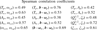
Table 1 collects the Spearman correlation coefficients estimated for pairs of quantities for which
 $C_{S}\gtrsim 0.4$
, namely if at least a significant moderate correlation is present. These also include the temperature anisotropy
 $A_{s}=T_{\bot ,s}/T_{\Vert ,s}$
, defined for both ion species, an important diagnostic for kinetic processes and instabilities. In the table, we have omitted the weakly correlated pairs, for which
 $C_{S}\lesssim 0.4$
.
Nonlinear Spearman correlation coefficients,
 $C_{S}$
, between pairs of quantities for which
 $C_{S}\gtrsim 0.4$
. All quantities are estimated using the HMV simulation results at
 $t=t^{\ast }$
.

To summarize the results of the above analysis, larger values of the deformation of the ion velocity and of the pressure tensor agyrotropy are recovered in spatial positions nearby the peaks of the ion vorticity and close to peaks of the current density. In these regions, differential heating and temperature anisotropy are also observed. Ion heating and kinetic effects are in general more strongly correlated with the vorticity than with the current density profile.
3 Local energy transfer rate in Vlasov–Maxwell simulations
3.1 Properties of the local energy transfer rate
Incompressible and isotropic MHD turbulence in plasmas can be described by the exact relation for the energy flux through the scales (see (1.1)). This Yaglom-like scaling law has been extensively tested in the solar wind, recovering very good agreements. The use of HVM multi-component simulation, described in § 2, can provide a better understanding of the connection between the MHD turbulent cascade and the relative kinetic effects on the ion velocity distributions since the in situ solar-wind measurements have several limitations.
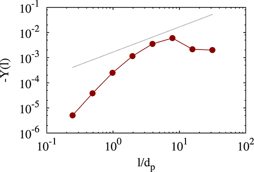
In figure 3, we present the validation of the PP law for the turbulent Vlasov simulation used in this work, as estimated by averaging (1.2). In the range of scales roughly corresponding to the inertial range of MHD turbulence, i.e. for
 $2d_{p}\lesssim l\lesssim 10d_{p}$
, the scaling of
 $-Y(l)$
is compatible with a linear law (figure 3). This suggests that the turbulent energy cascade is well developed in such range, at the time
 $t^{\ast }$
of the simulation. However, the limited extension of the inertial range does not allow a more precise and quantitative estimate (Parashar et al.
Reference Parashar, Matthaeus, Shay and Wan2015). It should be pointed out that the law as defined in (1.1), without absolute value, indicates the direction of the cascade towards small scales. The limited extension of the range observed in the HVM simulation may arise from several facts, which are physically meaningful. First, the system described here is size limited due to computational constraints: the correlation length is limited to roughly 10
 $d_{p}$
– relatively short as compared to the several decades of MHD turbulence commonly observed in the solar wind. Second, the PP law is exact only under the assumption of full isotropy, while our 2-D simulation has a mean magnetic field. Third, the ion skin depth is a characteristic length of the system, which breaks the validity of the MHD law. A more precise description could be obtained in terms of the Hall-MHD version of the PP law (Andrés et al.
Reference Andrés, Galtier and Sahraoui2018). This development is left for a future work. Fourth, in the derivation of these MHD-based scaling laws, isotropy of the pressure tensor is assumed, which does not hold in Vlasov turbulence. Finally, processes such as ion-cyclotron resonances and Landau damping might transfer free energy from the physical space to the velocity space, producing non-Maxwellian effects and, eventually, heating. All these caveats suggest that the analysis in terms of PP law and LET can only be meaningful for increments in the inertial range,
 $l>d_{p}$
. Therefore, part of our analysis will be performed using
 $l=2d_{p}$
.
Yaglom-law validation for turbulent Vlasov simulation (red markers and dashed line). The averaged scaling
 $Y=(Y^{+}+Y^{-})/2$
is shown using bi-logarithmic axes. The black dotted line represents an example of linear scaling, and is shown for reference only.

The local proxy
 $\unicode[STIX]{x1D716}_{l}(x,y)$
has been evaluated at different spatial scales
 $l$
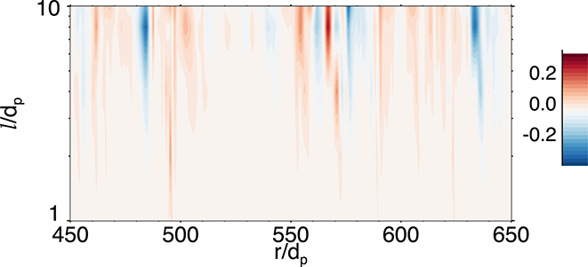
using the HVM simulation results. In figure 4 we show the scalogram of the LET
 $\unicode[STIX]{x1D716}_{l}$
along a one-dimensional cut of the 2-D spatial domain of the simulation. Note that a similar analysis has been performed for the PVI scalograms (Greco et al.
Reference Greco, Perri, Servidio, Yordanova and Veltri2016). Here we consider a diagonal path
 $r$
, normalized to
 $d_{p}$
, that crosses the simulation box several times. The channels of energy being transferred across scales are clearly visible, and reveal the complex, interwoven pattern of positive and negative flux that determines the neat energy flux (Coburn et al.
Reference Coburn, Smith, Vasquez, Forman and Stawarz2014; Sorriso-Valvo et al.
Reference Sorriso-Valvo, Carbone, Perri, Greco, Marino and Bruno2018).
The scalogram of LET
 $\unicode[STIX]{x1D716}_{l}$
, plotted as a colour map at different scales
 $l/d_{p}$
, estimated at different positions
 $r/d_{p}$
along a one-dimensional cut of the simulation domain. The alternate positive and negative energy transfer regions are evident.

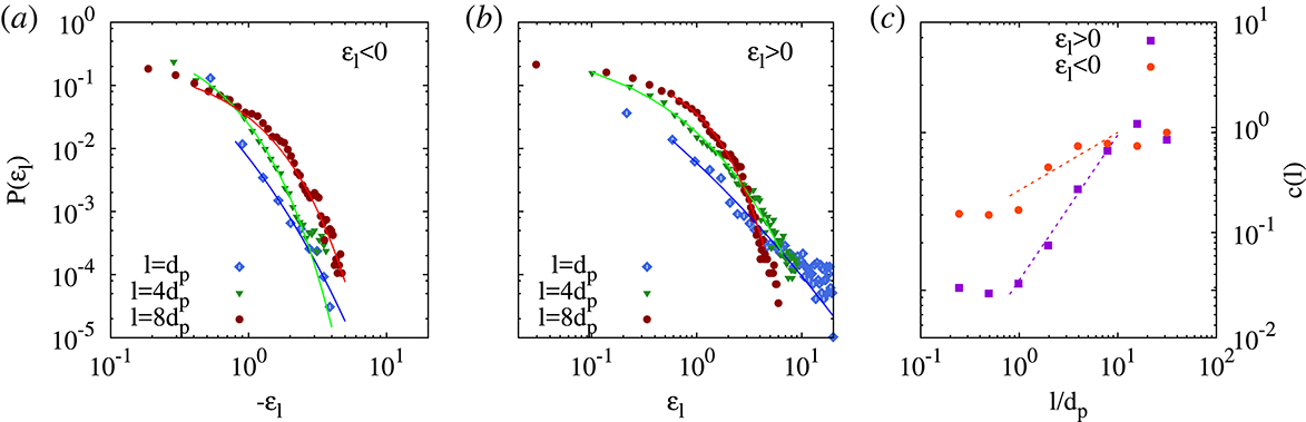
In order to characterize the statistical properties of the local energy transfer rate, in figure 5, we show the probability distribution functions (PDFs) of the negative (a) and positive (b) standardized LET values (i.e.
 $\unicode[STIX]{x1D716}_{l}(x,y)$
has been rescaled to have zero mean and unit standard deviation), for three different scales, namely
 $l=d_{p}$
(blue diamonds),
 $4d_{p}$
(green triangles) and
 $8d_{p}$
(red circles). In agreement with the PP law, for a given scale the positive tails are considerably higher and shallower than the negative ones, indicating the neat energy flux corresponding to the direct turbulent energy cascade towards small scales. This is clearly visible from the PDFs represented in figure 5.
Both positive and negative PDFs behave roughly as stretched exponential functions
 ${\sim}\exp (-b\unicode[STIX]{x1D716}_{l}^{c})$
, where
 $c$
is the parameter that controls the shape of the distribution tails. In particular,
 $c=2$
indicates a Gaussian tail,
 $c=1$
an exponential tail and for
 $c\rightarrow 0$
the tail approaches a power law. The curvature parameter
 $c$
, obtained from the fit at each scale, is shown in figure 5(c). Starting from the exponential value
 $c\sim 1$
at large scales (say for
 $l\gtrsim 10d_{p}$
), its value decreases with the scales, indicating the formation of highly localized small-scale structures, typical of intermittency. The two tails of the PDFs have different scaling, so that the positive tail has a more evident, faster decay than the negative tail. Such difference quantitatively confirms the imbalance already observed through the PDF shape. In the range corresponding to the MHD inertial range, the scaling of
 $c$
for the positive tail is well described by a power law
 $c_{\pm }^{\unicode[STIX]{x1D6FE}}$
, with exponent
 $\unicode[STIX]{x1D6FE}_{+}\sim 0.92\pm 0.06$
. For the negative tail, the scaling is less evident, but can be considered compatible with a power law with exponent
 $\unicode[STIX]{x1D6FE}_{-}\sim 0.37\pm 0.13$
. This confirms that the numerical simulation has reached a stage of fully developed turbulence, with a strongly intermittent energy cascade, whose characteristics are well captured by the LET. Note that a similar behaviour has been recently observed in solar-wind measurements (Sorriso-Valvo et al.
Reference Sorriso-Valvo, Carbone, Perri, Greco, Marino and Bruno2018). At smaller scales, for
 $l\lesssim d_{p}$
, the parameter seems to reach a limiting value for both the positive and negative tails, indicating the saturation of intermittency. In this short range of scales, the positive tail of the PDF is described by
 $c\sim 0.1$
, closer to power-law decay. The negative tail converges towards a slightly larger value
 $c\sim 0.3$
, indicating a faster than power-law decay, and confirming once more the quantitative difference between positive and negative energy transfer rate.
In (a), the probability distribution functions (PDFs) of the standardized, negative
 $\unicode[STIX]{x1D716}_{l}(x,y)$
are shown for three different scales, namely
 $l=d_{p}$
(blue diamonds),
 $4d_{p}$
(green triangles) and
 $8d_{p}$
(red circles), using logarithmic axes. In (b), the PDFs of positive
 $\unicode[STIX]{x1D716}_{l}(x,y)$
are shown for the same scales, with the same symbols. In both panels, the different lines are the stretched exponential fits, obtained through a standard least-
 $\unicode[STIX]{x1D712}^{2}$
procedure. (c) Shows the scaling properties of the curvature parameter
 $c(l)$
, for the positive (violet squares) and negative (orange circles) tails of the PDFs. The inertial-range power-law fits are also indicated as dashed lines, the scaling exponents being respectively
 $\unicode[STIX]{x1D6FE}_{+}=0.92$
and
 $\unicode[STIX]{x1D6FE}_{-}=0.37$
.

3.2 Conditioned analysis of kinetic quantities
After establishing the statistical properties of the LET in our hybrid simulation, we have performed the conditioned average analysis proposed by Osman et al. (Reference Osman, Matthaeus, Hnat and Chapman2012), and recently performed using the LET (Sorriso-Valvo et al.
Reference Sorriso-Valvo, Carbone, Perri, Greco, Marino and Bruno2018). The conditioned analysis is designed to highlight the existence of robust features in the data that might be hidden by the turbulent fluctuations. To this goal, we have selected different values of threshold
 $\unicode[STIX]{x1D703}_{d_{p}}$
of the LET
 $\unicode[STIX]{x1D716}_{d_{p}}$
, estimated at the bottom of the inertial range
 $l\simeq 2d_{p}$
, to identify locations associated with large energy flux at the end of the fluid-like nonlinear turbulent cascade.
Then, for each threshold, some of the variables described in § 2 have been averaged only in those locations where the LET overcomes the threshold:
 $\unicode[STIX]{x1D716}_{d_{p}}\geqslant \unicode[STIX]{x1D703}_{d_{p}}$
for positive thresholds (cascade towards smaller scales), and
 $\unicode[STIX]{x1D716}_{d_{p}}\leqslant \unicode[STIX]{x1D703}_{d_{p}}$
for negative thresholds (cascade towards higher scales). This gives the conditionally averaged values, for example
 $\langle T_{p}|\unicode[STIX]{x1D703}_{d_{p}}\rangle$
in the case of the proton temperature.
Through the above procedure, the turbulent fluctuations are all averaged to their mean value, except where systematic variations are present. The same procedure is repeated using all the points located at a given distances
 $\unicode[STIX]{x1D6FF}$
from the location of large LET, and for different values of
 $\unicode[STIX]{x1D6FF}$
. This provides the average profile of the physical quantities in the vicinity of the bursts of energy flux, as a function of the distance from the LET burst. By repeating the same analysis using different thresholds, it is then possible to determine the role of the energy flux in the robust modification of the physical quantities.
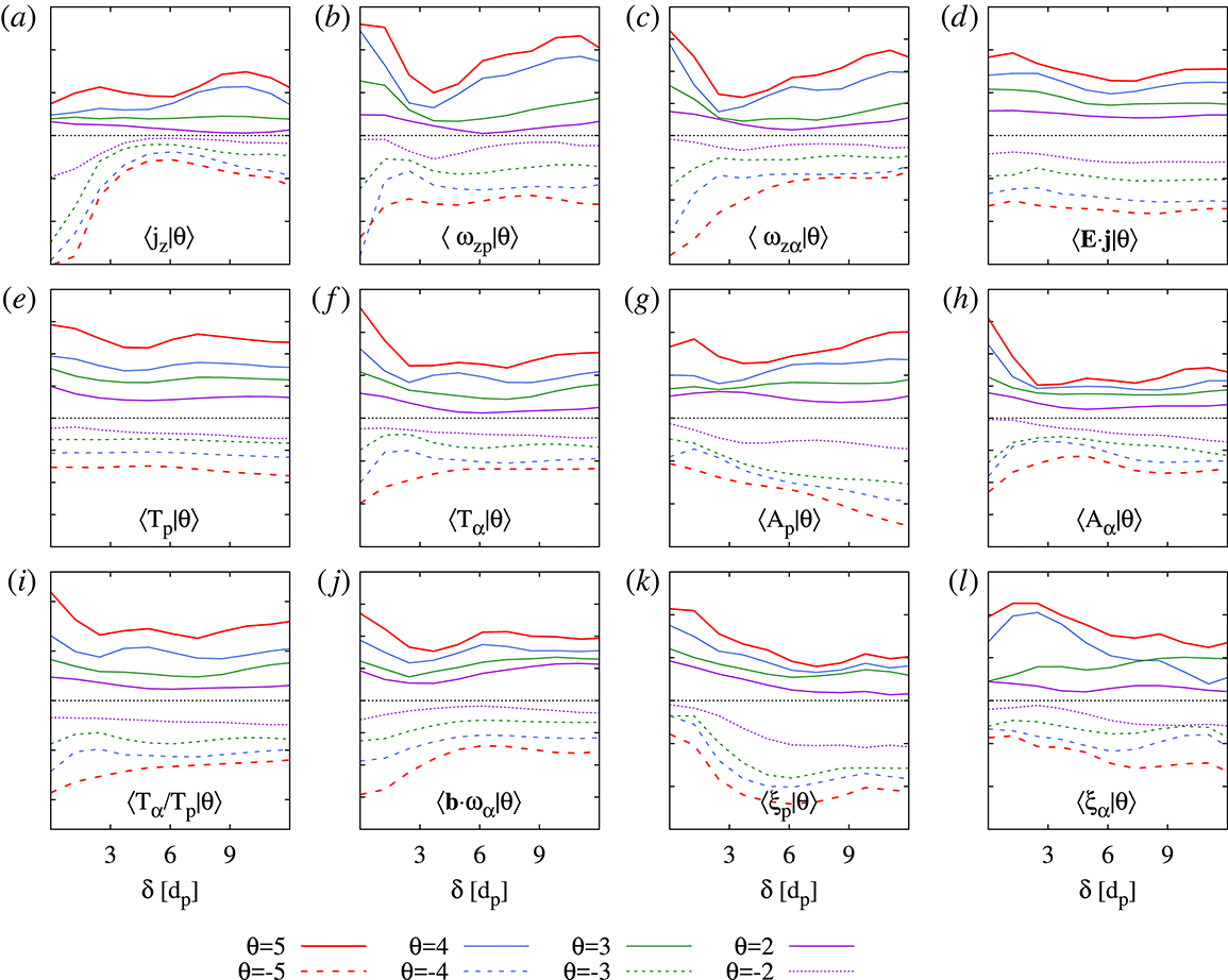
Figure 6(a–l) show the conditioned average profiles obtained using the HVM simulation results, for some of the physical quantities described in § 2 and indicated in each panel. The average has been computed up to a distance
 $\unicode[STIX]{x1D6FF}=12d_{p}$
from the LET peaks. For each panel, the different line styles refer to the different threshold values, as listed at the bottom of the figure. All curves have been vertically shifted for clarity, and are therefore given in arbitrary units. The dotted horizontal line has the only purpose of separating the positive from the negative threshold values. The figure shows that most of the variables have a clear enhancement at
 $\unicode[STIX]{x1D6FF}=0$
in the positive LET peak cases, which is more evident for larger threshold values. At the same time, in most cases the negative LET peaks are associated with a reduction of the conditioned average, again more evident for larger negative thresholds. This observation generally suggests that kinetic processes are more effective within a few
 $d_{p}$
from the intermittent structures, or more precisely from the locations where the fluid-scale turbulent cascade has produced a larger flux of energy.
Conditionally averaged quantities as a function of the distance from the peak of the LET, estimated at the scale
 $l\simeq 2d_{p}$
, for four positive and four negative LET threshold values
 $\unicode[STIX]{x1D703}_{d_{p}}$
(coded in different line colours, as indicated at the bottom of the figure). Each panel refers to one of the physical quantities (see § 2, given in the legend located at the bottom of the panel). All curves have been vertically shifted for clarity, and are thus presented in arbitrary units. In each panel, the curves for larger positive thresholds (full lines) are those shown at upper positions, and the larger negative thresholds (dashed lines) are shown at lower positions. The dotted horizontal line has the sole purpose of separating the curves relative to positive (above the line) and negative (below the line) thresholds.

A more detailed look at the individual panels of figure 6 can provide information that may help uncovering the kinetic processes occurring in the simulation. (a) Shows that the off-plane current
 $j_{z}$
is not well co-located with the positive LET structures, as the conditioned average profiles show a weak peak near
 $\unicode[STIX]{x1D6FF}\simeq 3d_{p}$
. Note that conditioning the average
 $j_{z}$
to large values of the LET estimated at the smallest scale in the simulation results in larger correlations than at
 $l=2d_{p}$
. This is to be expected, and possibly trivial, as the contribution to the LET of the LET term including
 $\unicode[STIX]{x0394}b^{2}$
(strongly correlated to
 $j_{z}$
) and
 $\unicode[STIX]{x0394}v^{2}$
(strongly correlated to
 $\unicode[STIX]{x1D714}_{z}$
) would dominate, since the other term (including the
 $\unicode[STIX]{x0394}v\cdot \unicode[STIX]{x0394}b$
correlations) becomes less meaningful. On the contrary, regions of strong negative LET are associated with smaller current, as evident from the bottom part of (a). This could arise from the fact that negative LET structures are associated with regions where the turbulent production of small scales is locally inhibited, indicating possible equilibrium-like patterns, that results from a process of suppression of nonlinearity (Servidio et al.
Reference Servidio, Matthaeus and Dmitruk2008).
In (b,c), the average proton and
 $\unicode[STIX]{x1D6FC}$
particle vorticity peak at large positive LET locations, and, as for the current, is minimal for large negative LET. This observation confirms previous results, obtained using particle-in-cell simulations, which show that correlations between vorticity structures and kinetic features are stronger than for the current structures (Parashar & Matthaeus Reference Parashar and Matthaeus2016).
Figure 6(d) shows that the exchange of energy between particles and fields, represented here through the quantity
 $\boldsymbol{E}\boldsymbol{\cdot }\boldsymbol{j}$
, is weakly enhanced near the LET positive peaks, but is relatively unaffected by the presence of negative LET peaks. This is in good agreement with previous works, where it has been shown that locally the cascade produces narrow heating and dissipation patterns (Karimabadi et al.
Reference Karimabadi, Roytershteyn, Wan, Matthaeus, Daughton, Wu, Shay, Loring, Borovsky and Leonardis2013).
Figure 6(e,f) display enhanced temperature near the positive LET peaks for both species, which extends up
 $\unicode[STIX]{x1D6FF}\sim$
2–3
 $d_{p}$
from the peaks. For the
 $\unicode[STIX]{x1D6FC}$
particles, there is indication of colder temperature near the large negative LET points, which highlights the possible presence of a differential heating processes of the two species (Kasper et al.
Reference Kasper, Lazarus and Gary2008; Maruca et al.
Reference Maruca, Kasper and Gary2012).
Figure 6(g,h) show the conditioned profiles of the temperature anisotropy
 $A_{s}$
. In (g), the proton temperature anisotropy is only weakly affected by large positive energy transfer, while a general anisotropy increase can be observed in correspondence with large negative LET. On the contrary, as can be seen in (h), the
 $\unicode[STIX]{x1D6FC}$
particle temperature anisotropy increases (decrease) near the large positive (negative) LET structures. In this case, the LET dependence is similar for the temperature anisotropy and for the total temperature. This suggests that the presence of large turbulent energy transfer increases predominantly the perpendicular temperature, indicating for example the possible role of ion-cyclotron or mirror instabilities (Matteini et al.
Reference Matteini, Hellinger, Goldstein, Landi, Velli and Neugebauer2013).
Figure 6(i) quantifies the strong enhancement of the temperature ratio
 $T_{\unicode[STIX]{x1D6FC}}/T_{p}$
near the sites of strong positive energy transfer, and the corresponding decrease at the negative LET peaks. This plot magnifies the difference in the conditionally averaged temperature for the two species, seen in (e,f), and confirms the relevance of differential heating at the sites of strong turbulent activity.
Figure 6(j) shows that the quantity
 $\boldsymbol{b}\boldsymbol{\cdot }\unicode[STIX]{x1D714}_{s}$
has similar conditioned averages as for the vorticity (see b,c), for both protons (not shown) and
 $\unicode[STIX]{x1D6FC}$
particles.
Finally, (k,l) show that the parameter
 $\unicode[STIX]{x1D709}_{s}$
, quantifying the general deviation from Maxwellian velocity distribution function (VDF), is clearly larger at both positive and negative LET structures, and for both ion species. This last observation confirms that the kinetic processes resulting in modification of the ion VDFs are predominantly seen in the proximity of the locations with enhanced turbulent energy flux, where free energy is available for small-scale processes to occur. Additionally, it suggests that regions characterized by absent or reduced direct energy transfer towards small scales (large negative LET) are also characterized by the presence of robustly non-Maxwellian VDF. Whether this indicates that kinetic effect may provide feedback to the larger scales through some form of inverse cascade remains an open question that deserves further analysis.
It is interesting but not surprising to note that, for most of the physical quantities studied here, the observed peaks extend to approximately 2–3
 $d_{p}$
around the LET structures. This indicates that the effects of the kinetic features are typically smeared out within such range.
4 Conclusions
Exploring the details of the cross-scale connections between the MHD turbulent energy cascade and the small-scale kinetic processes is an important key to understand the role of dissipation mechanisms in collisionless plasmas (Schwartz et al. Reference Schwartz, Hellinger, Bale, Owen, Nakamura, Vaivads, Sorriso-Valvo, Liu, Wimmer-Schweingruber and Fujimoto2011; Alexandrova et al. Reference Alexandrova, Chen, Sorriso-Valvo, Horbury and Bale2013; Chen Reference Chen2016). Numerical simulations can provide important insight into general processes, in particular when experimental systems and observations are not easily controlled.
In this article, we have presented the analysis of one snapshot in the quasi-steady state turbulence of a two-dimensional hybrid Vlasov–Maxwell numerical simulation (HVM), with the inclusion of
 $\unicode[STIX]{x1D6FC}$
particles. The range of scales that have been investigated includes both the fluid range, where MHD turbulence transfers energy across scales, and the sub-ion range, where kinetic effects dominate the dynamics. This multi-scale investigation allows us to explore the role of the turbulent energy that reaches the typical ion scales in highly localized regions of space (both in the form of coherent structures and of correlated fluctuations) and the kinetic processes occurring at small scales. The former is represented by means of a proxy of the local energy transfer rate (LET), whose heuristic definition is based on the linear scaling laws of the mixed third-order moment of the MHD fluctuations, and which carries more details on the type of fluctuations associated with the energy transfer with respect to other proxies (e.g. the PVI). The latter are described here through several quantities that can be related to kinetic processes, as for example the ion temperature and its anisotropy with respect to the magnetic field direction, or an index of deviation from Maxwellian particle velocity distribution.
We have initially described the correlations between such kinetic quantities, first by visually comparing their maps, then by looking at some examples of joint probability distributions of such quantities pairs, and finally by estimating the nonlinear correlation coefficients between all the pairs. Several diagnostics show significant correlation. For example, the ion vorticity and the associated temperature show moderate correlation for both species, confirming previous observations that the temperature is enhanced in correspondence of vorticity structures (Servidio et al. Reference Servidio, Valentini, Perrone, Greco, Califano, Matthaeus and Veltri2015; Franci et al. Reference Franci, Hellinger, Matteini, Verdini, Landi and Wang2016; Parashar & Matthaeus Reference Parashar and Matthaeus2016; Valentini et al. Reference Valentini, Perrone, Stabile, Pezzi, Servidio, De Marco, Marcucci, Bruno, Lavraud and De Keyser2016). The deviation from Maxwellian (Servidio et al. Reference Servidio, Valentini, Califano and Veltri2012; Valentini et al. Reference Valentini, Perrone, Stabile, Pezzi, Servidio, De Marco, Marcucci, Bruno, Lavraud and De Keyser2016) is also very well correlated with the pressure tensor anisotropy, revealing its relevant contribution in determining such deviation.
We have then analysed the statistical properties of the energy transfer rate in HVM turbulence. The domain-averaged third-order moment suggests that the turbulent cascade might be fully developed in the range approximately between
 ${\sim}2d_{p}$
and
 ${\sim}10d_{p}$
, where the measured energy flux is compatible with linear scaling. A direct cascade of energy is present (the negative sign of the third-order moment
 $Y$
), in agreement with the expectations for turbulence in the MHD inertial range of scales. However, looking at the space-scale distribution of the local contributions to such scaling law, it is clear that both positive and negative energy fluxes exist, and are in comparable quantity, all across the simulation domain, the negative sign being the global balance between those.
The scaling properties of the LET were modelled in terms of stretched exponential distributions, which provided a satisfactory description of the PDFs at all scales. The imbalance between positive and negative values of
 $\unicode[STIX]{x1D716}$
are well described by the asymmetry of their distributions. Moreover, the shape parameter of the fitted distributions shows power-law scaling in the inertial range, in agreement with previous observations of solar-wind turbulence (Sorriso-Valvo et al.
Reference Sorriso-Valvo, Carbone, Perri, Greco, Marino and Bruno2018) and confirming the reliability of the proxy for the description of the turbulence properties.
Finally, we have explored the presence of correlations between the LET and the quantities described before. To this aim, we have calculated the conditionally averaged profile of each of those quantity, around the locations where the LET exceeds some given thresholds (Osman et al. Reference Osman, Matthaeus, Hnat and Chapman2012; Sorriso-Valvo et al. Reference Sorriso-Valvo, Carbone, Perri, Greco, Marino and Bruno2018). This analysis may provide more detailed information that can help understand which kinetic processes are responsible for the removal (or transformation) of the turbulent energy from the system. These profiles shows that most of the physical quantities related to ‘dissipative’ or kinetic processes are enhanced near regions of large positive LET, indicating a large flux of energy towards small scales. Conversely, these are often reduced near strong negative LET, likely associated with energy being transferred towards large scales, and thus indicating less availability of energy in the kinetic range.
Our results suggest, for example, that peaks of turbulent energy transfer are associated with enhanced temperature. More in particular, the perpendicular temperature increases near the high LET locations, indicating the possible role of ion-cyclotron or mirror instabilities (Matteini et al.
Reference Matteini, Hellinger, Goldstein, Landi, Velli and Neugebauer2013). The typical size of the region where the enhancement is observed is, for most quantities, of the order of 2–3
 $d_{p}$
, while at larger distance their persistent fluctuations are averaged out. It is also clear from the analysis that the vorticity is a better tracer of energy availability than the current density (Servidio et al.
Reference Servidio, Valentini, Perrone, Greco, Califano, Matthaeus and Veltri2015; Franci et al.
Reference Franci, Hellinger, Matteini, Verdini, Landi and Wang2016; Parashar & Matthaeus Reference Parashar and Matthaeus2016; Valentini et al.
Reference Valentini, Perrone, Stabile, Pezzi, Servidio, De Marco, Marcucci, Bruno, Lavraud and De Keyser2016), and that correlations are more evident for the
 $\unicode[STIX]{x1D6FC}$
particles than for protons (Valentini et al.
Reference Valentini, Perrone, Stabile, Pezzi, Servidio, De Marco, Marcucci, Bruno, Lavraud and De Keyser2016). Finally, deviations from Maxwellian VDF are evident for both positive and negative peaks of LET, an interesting feature that deserves further analysis.
The study of the local properties of the turbulent cascade can be a valuable tool for the exploration of the kinetic-range processes in space plasmas. The validation of its use in numerical simulations provided in this work suggests its possible use with the recently available high-quality plasma measurements in the solar wind and in the magnetosphere, provided by the Multiscale Magnetospheric mission MMS (Burch et al. Reference Burch, Moore, Torbert and Giles2016a ). Extension to more complete descriptions of the energy transfer rate could be also used, allowing us, for example, to examine the actual role played by compressive effects (Carbone Reference Carbone, Marino, Sorriso-Valvo, Noullez and Bruno2009; Andrés et al. Reference Andrés, Galtier and Sahraoui2018).
Acknowledgements
This work has been partly supported by the Agenzia Spaziale Italiana under the contract no. ASI-INAF 2015-039-R.O ‘Missione M4 di ESA: Partecipazione Italiana alla fase di assessment della missione THOR’ and by the International Space Science Institute (ISSI) in the framework of International Team 504 entitled ‘Current Sheets, Turbulence, Structures and Particle Acceleration in the Heliosphere’. L.S.-V., D.P., S.S. and I.Z. acknowledge support from the Faculty of the European Space Astronomy Centre (ESAC). Numerical simulations here discussed have been run on the Newton parallel machine at the University of Calabria (Italy).