1 Introduction
Understanding the configuration and evolution of magnetic structures in magnetohydrodynamic (MHD) flows is of fundamental importance for device design and stability analysis in nuclear fusion (e.g. Kruskal et al. Reference Kruskal, Johnson, Gottlieb and Goldman1958; Liewer Reference Liewer1985; Nelson et al. Reference Nelson, Jarboe, Martin, Orvis, Xie, Zhang and Zhou1995; Dinklage et al. Reference Dinklage, Beidler, Helander, Fuchert, Maassberg, Rahbarnia, Pedersen, Turkin, Wolf and Alonso2018) and corona dynamics in astrophysics (e.g. Low Reference Low1996; Braithwaite Reference Braithwaite2009; Yang et al. Reference Yang, Büchner, Santos and Zhang2013; Wang et al. Reference Wang, Cao, Liu, Xu, Liu, Zeng, Chae and Ji2015; Amari et al. Reference Amari, Canou, Aly, Delyon and Alauzet2018; Inoue et al. Reference Inoue, Kusano, Büchner and Skála2018). As representative simplified magnetic structures, several analytical models have been developed for specific magnetic configurations, such as toroidal and knotted confinement vessels (e.g. Taylor Reference Taylor1974; Hudson, Startsev & Feibush Reference Hudson, Startsev and Feibush2014) and unbounded force-free fields (e.g. Marsh Reference Marsh1996).
The knotted flux tube is a typical magnetic configuration with non-trivial topology and relatively simple geometry, so it is often used for investigating essential dynamics in MHD flows (e.g. Arrayás, Bouwmeester & Trueba Reference Arrayás, Bouwmeester and Trueba2017). Moreover, the importance of knots has been underscored in various physical systems, such as classical fluids (Kleckner & Irvine Reference Kleckner and Irvine2013), quantum fluids (Kleckner, Kauffman & Irvine Reference Kleckner, Kauffman and Irvine2016), optical fields (Dennis et al. Reference Dennis, King, Jack, O’Holleran and Padgett2010) and liquid crystals (Martinez et al. Reference Martinez, Ravnik, Lucero, Visvanathan, Z̆umer and Smalyukh2014). In particular, the evolution of magnetic knots in MHD is sensitive to the twist of field lines within the flux tube (see Candelaresi, Sordo & Brandenburg Reference Candelaresi, Sordo and Brandenburg2010; Smiet et al. Reference Smiet, Candelaresi, Thompson, Swearngin, Dalhuisen and Bouwmeester2015), but there is a lack of general methods for constructing knotted flux tubes with arbitrary shape and twist.
For characterizing knotted fields, helicity is a topological measure of the linking and knotting of field lines, and it is a conserved quantity in ideal MHD flows (see Woltjer Reference Woltjer1958; Moreau Reference Moreau1961; Moffatt Reference Moffatt1969), so it is an important constraint to elucidate the evolution mechanisms of magnetic structures. The helicity of an isolated flux tube depends on the geometry, topology and magnetic distribution of field lines within the tube, and its explicit expression is generally hard to derive except for some special cases. For an unknotted magnetic ring consisting of nested toroidal magnetic surfaces, the helicity can be derived based on toroidal and poloidal magnetic fluxes (Kruskal & Kulsrud Reference Kruskal and Kulsrud1958; Berger & Field Reference Berger and Field1984). This explicit expression was generalized to knotted flux tubes by introducing a ‘zero-framed’ coordinate system in Chui & Moffatt (Reference Chui and Moffatt1995) and Maggioni & Ricca (Reference Maggioni and Ricca2009). In general, coiling and twisting of flux tubes are two ingredients determining the helicity (see Berger Reference Berger1999; Scheeler et al. Reference Scheeler, Kleckner, Proment, Kindlmann and Irvine2014, Reference Scheeler, van Rees, Kedia, Kleckner and Irvine2017; Kerr Reference Kerr2018a), but it is difficult to isolate each of them in quantitative analysis.
Thus the construction of knotted flux tubes with an explicit helicity is valuable for quantitative study. There are two theoretical approaches for constructing flux tubes, via the parametric equation and Clebsch potentials. In the former one, Xiong & Yang (Reference Xiong and Yang2019a) extended the method of Chui & Moffatt (Reference Chui and Moffatt1995) to construct the solenoidal vector fields for knotted vortex/flux tubes by specifying the parametric equation of the tube axis and the magnitude distribution within the tube. However, the intrinsic twist of field lines (see Moffatt & Ricca Reference Moffatt and Ricca1992) is not considered in this method. The twist of vortex lines can decay rapidly in viscous hydrodynamic (HD) flows (see Scheeler et al. Reference Scheeler, Kleckner, Proment, Kindlmann and Irvine2014), whereas the twist of field lines can have an impact on magnetic dynamics in MHD flows.
In the latter approach via Clebsch potentials, a solenoidal vector field is mapped to a specific geometric structure using various transformations. In the representation of Clebsch (Reference Clebsch1859), the vector field with vanishing helicity can be locally expressed by a mapping of two scalar potential functions. The Clebsch map containing important geometric information of the vector field is useful for diagnostics and visualization of fluid dynamics (e.g. Yang & Pullin Reference Yang and Pullin2010; Chern et al. Reference Chern, Knöppel, Pinkall and Schröder2017), and it has been augmented into several variants allowing non-vanishing helicity of constructed fields, e.g. the  $n$-dimensional Clebsch map (Zakharov & Kuznetsov Reference Zakharov and Kuznetsov1997; Cartes, Bustamante & Brachet Reference Cartes, Bustamante and Brachet2007), spherical Clebsch map (see Kamchatnov Reference Kamchatnov1982; Chern et al. Reference Chern, Knöppel, Pinkall, Schröder and Weissmann2016, Reference Chern, Knöppel, Pinkall and Schröder2017) and rational maps (see Kedia et al. Reference Kedia, Foster, Dennis and Irvine2016). A major issue of the methods via Clebsch-like maps is the lack of general construction methods for scalar potentials.
The evolution of knotted flux tubes contains essential dynamics in plasmas. For ideal MHD with vanishing magnetic diffusivity, Woltjer (Reference Woltjer1958) proved that a force-free or Beltrami state is the lowest-energy configuration for magnetic fields under the constraint of helicity conservation. Taylor (Reference Taylor1974) conjectured that the plasma with a very low resistivity in a toroidal device relaxes to a lower-energy, linear force-free state under helicity conservation. Moffatt (Reference Moffatt1990) argued that the minimum energy in the relaxation of magnetic knots is solely determined by the topology of the knots. Ricca (Reference Ricca2008) further proved that the minimum energy of zero-framed knots/links is provided by the topological crossing number. Smiet, Candelaresi & Bouwmeester (Reference Smiet, Candelaresi and Bouwmeester2017) found an equilibrium plasma configuration characterized by a lowered pressure in a toroidal region, with field lines lying on surfaces of constant pressure.
For resistive MHD with finite diffusivity, the evolution of magnetic structures can be much more complex than those in ideal MHD flows owing to magnetic reconnection (see Taylor Reference Taylor1986; Biskamp Reference Biskamp1997; Zweibel & Yamada Reference Zweibel and Yamada2016). Beyond the conjecture of Taylor (Reference Taylor1974), recent simulations of flux tubes showed additional topological constraints hindering the relaxation to a force-free state (see Yeates, Hornig & Wilmot-Smith Reference Yeates, Hornig and Wilmot-Smith2010; Smiet et al. Reference Smiet, Candelaresi, Thompson, Swearngin, Dalhuisen and Bouwmeester2015), but the detailed dynamics of flux tubes and its relation to helicity components has not been fully elucidated owing to the insufficient accuracy for numerical construction of knotted flux tubes.
In the present study, we extend the methods of Gold & Hoyle (Reference Gold and Hoyle1960) and Xiong & Yang (Reference Xiong and Yang2019a) to construct knotted flux tubes with arbitrary shape and tunable twist. The central axis of the constructed tube is prescribed by a smooth and non-degenerate closed curve. The helicity and its components have explicit expressions, so we can isolate the effects of coiling and twisting of field lines on the magnetic evolution. Furthermore, we develop an accurate numerical algorithm to construct divergence-free and compactly supported vector fields of knotted flux tubes in Cartesian coordinates. The constructed vector fields can be used as the initial magnetic induction or vorticity field in the direct numerical simulation (DNS) of MHD or HD flows, respectively. In particular, we reveal the effects of the initial twist of field lines on the evolution of trefoil flux tubes, and elucidate the mechanism of topological changes of magnetic fields in resistive MHD.
The outline of this paper is as follows. In § 2, we develop a general method to construct the solenoidal vector field for a knotted flux tube from a given parametric curve, and then derive the expressions for the helicity and its components. Next, § 3 describes numerical methods and set-ups in the DNS of trefoil flux tubes with various twist degrees in MHD flows. In § 4, we elucidate the effects of twist on major statistics and structural changes in the evolution of knotted flux tubes. Some conclusions are drawn in § 5.
2 Construction of coiled and twisted flux tubes
2.1 Parametric curve and coordinate systems
The flux tube is constructed from a given continuous and differentiable closed curve  $C$ without vanishing curvature in three-dimensional Euclidean space
 $\unicode[STIX]{x211D}^{3}$. The parametric equation of
 $C$ is
 $\boldsymbol{x}=\boldsymbol{c}(s)$, where
 $\boldsymbol{x}=(x,y,z)$ denotes spatial Cartesian coordinates and
 $s\in [0,L_{C})$ is the arclength parameter with the length
 $L_{C}$ of
 $C$. The Frenet–Serret frame on
 $C$ is
 $$\begin{eqnarray}\left.\begin{array}{@{}c@{}}{\displaystyle \frac{\text{d}\boldsymbol{T}}{\text{d}s}}=\unicode[STIX]{x1D705}\boldsymbol{N},\\ {\displaystyle \frac{\text{d}\boldsymbol{N}}{\text{d}s}}=-\unicode[STIX]{x1D705}\boldsymbol{T}+\unicode[STIX]{x1D70F}\boldsymbol{B},\\ {\displaystyle \frac{\text{d}\boldsymbol{B}}{\text{d}s}}=-\unicode[STIX]{x1D70F}\boldsymbol{N},\end{array}\right\}\end{eqnarray}$$
where  $\boldsymbol{T}\equiv \text{d}\boldsymbol{c}/\text{d}s$ denotes the unit tangent,
 $\boldsymbol{N}\equiv (\text{d}\boldsymbol{T}/\text{d}s)/|\text{d}\boldsymbol{T}/\text{d}s|$ the unit normal,
 $\boldsymbol{B}\equiv \boldsymbol{T}\times \boldsymbol{N}$ the unit binormal,
 $\unicode[STIX]{x1D705}$ the curvature and
 $\unicode[STIX]{x1D70F}$ the torsion of the curve.
To facilitate the construction of vector field  $\boldsymbol{{\mathcal{B}}}$ for the flux tube, we introduce a curved cylindrical coordinate system
 $(s,\unicode[STIX]{x1D70C},\unicode[STIX]{x1D703})$ in a tubular region surrounding curve
 $C$ (see Chui & Moffatt Reference Chui and Moffatt1995). The system satisfies
 $$\begin{eqnarray}\boldsymbol{x}=\boldsymbol{c}(s)+\unicode[STIX]{x1D70C}\cos \unicode[STIX]{x1D703}\,\boldsymbol{N}(s)+\unicode[STIX]{x1D70C}\sin \unicode[STIX]{x1D703}\,\boldsymbol{B}(s).\end{eqnarray}$$
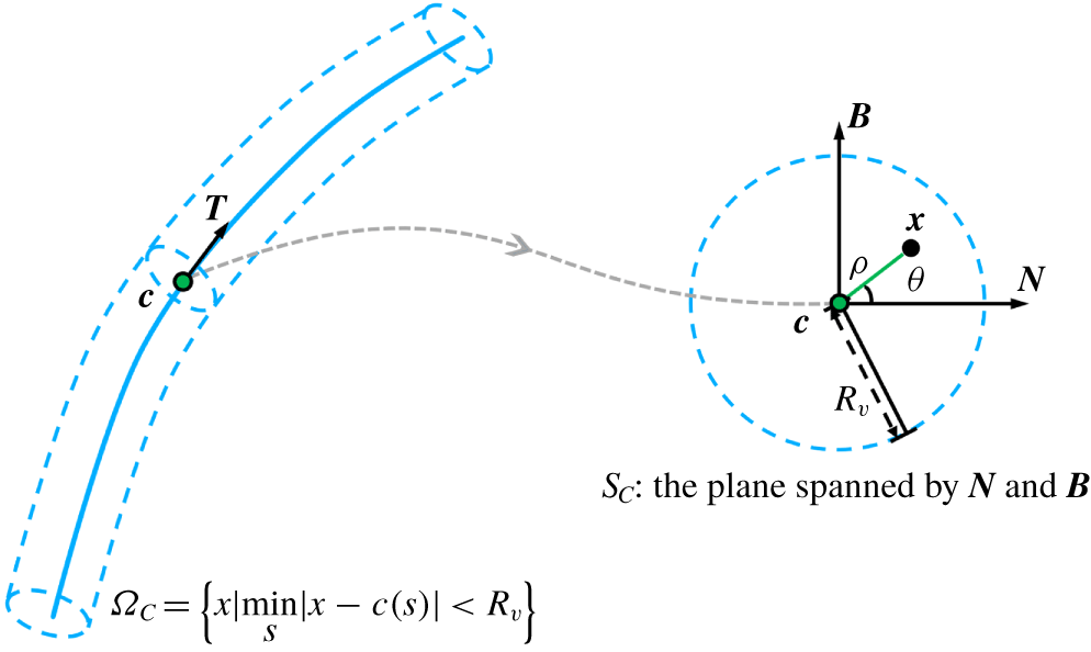
As sketched in figure 1,  $\boldsymbol{x}-\boldsymbol{c}(s)$ is perpendicular to
 $\boldsymbol{T}(s)$,
 $\unicode[STIX]{x1D70C}$ denotes the radial distance from
 $\boldsymbol{c}(s)$ and
 $\unicode[STIX]{x1D703}$ denotes the azimuthal angle from
 $\boldsymbol{N}(s)$ in the plane
 $S_{C}$ spanned by
 $\boldsymbol{N}(s)$ and
 $\boldsymbol{B}(s)$. We specify
 $\boldsymbol{{\mathcal{B}}}$ in terms of
 $(s,\unicode[STIX]{x1D70C},\unicode[STIX]{x1D703})$ in the tubular region,
 $$\begin{eqnarray}\unicode[STIX]{x1D6FA}_{C}=\left\{\boldsymbol{x}\,\Big|\,\boldsymbol{x}\in \unicode[STIX]{x211D}^{3},~\min _{s}|\boldsymbol{x}-\boldsymbol{c}(s)|<R_{v}\right\},\end{eqnarray}$$
where curve  $C$ is the central axis, and
 $R_{v}$ denotes the radius of
 $\unicode[STIX]{x1D6FA}_{C}$ and is set to be small enough so that
 $s$ is uniquely determined by (2.2) (see Xiong & Yang Reference Xiong and Yang2019a).
Schematic diagram of the relation between coordinates  $(s,\unicode[STIX]{x1D70C},\unicode[STIX]{x1D703})$ and
 $(x,y,z)$. The flux tube is sketched by dashed curves, and its central axis is marked by the blue solid curve.

Within  $\unicode[STIX]{x1D6FA}_{C}$, the coordinate systems
 $\boldsymbol{x}$ and
 $(s,\unicode[STIX]{x1D70C},\unicode[STIX]{x1D703})$ are convertible except for the
 $\unicode[STIX]{x1D703}$-component on
 $C$. Xiong & Yang (Reference Xiong and Yang2019a) proved that
 $(s,\unicode[STIX]{x1D70C})$ determined by (2.2) in
 $\unicode[STIX]{x1D6FA}_{C}$ satisfies
 $$\begin{eqnarray}\left.\begin{array}{@{}c@{}}s=\displaystyle \text{arg min}_{\unicode[STIX]{x1D701}}|\boldsymbol{x}-\boldsymbol{c}(\unicode[STIX]{x1D701})|,\\ \unicode[STIX]{x1D70C}=\displaystyle \text{min}_{\unicode[STIX]{x1D701}}|\boldsymbol{x}-\boldsymbol{c}(\unicode[STIX]{x1D701})|,\end{array}\right\}\end{eqnarray}$$
and the azimuthal coordinate can be expressed as
 $$\begin{eqnarray}\unicode[STIX]{x1D703}=\arccos \frac{[\boldsymbol{x}-\boldsymbol{c}(s)]\boldsymbol{\cdot }\boldsymbol{N}(s)}{\unicode[STIX]{x1D70C}}.\end{eqnarray}$$
2.2 Knotted vector field with tunable twist
We develop a general method for constructing a solenoidal vector field
 $$\begin{eqnarray}\boldsymbol{{\mathcal{B}}}=b^{s}(s,\unicode[STIX]{x1D70C},\unicode[STIX]{x1D703})\boldsymbol{e}_{s}+b^{\unicode[STIX]{x1D70C}}(s,\unicode[STIX]{x1D70C},\unicode[STIX]{x1D703})\boldsymbol{e}_{\unicode[STIX]{x1D70C}}+b^{\unicode[STIX]{x1D703}}(s,\unicode[STIX]{x1D70C},\unicode[STIX]{x1D703})\boldsymbol{e}_{\unicode[STIX]{x1D703}}\end{eqnarray}$$
in  $\unicode[STIX]{x1D6FA}_{C}$ on the local frame spanned by unit vectors
 $$\begin{eqnarray}\left.\begin{array}{@{}c@{}}\boldsymbol{e}_{s}=\boldsymbol{T},\\ \boldsymbol{e}_{\unicode[STIX]{x1D70C}}=\cos \unicode[STIX]{x1D703}\boldsymbol{N}+\sin \unicode[STIX]{x1D703}\boldsymbol{B},\\ \boldsymbol{e}_{\unicode[STIX]{x1D703}}=-\sin \unicode[STIX]{x1D703}\boldsymbol{N}+\cos \unicode[STIX]{x1D703}\boldsymbol{B},\end{array}\right\}\end{eqnarray}$$
for the knotted flux tube with finite thickness and tunable twist, where  $b^{s}$,
 $b^{\unicode[STIX]{x1D70C}}$ and
 $b^{\unicode[STIX]{x1D703}}$ are the components of
 $\boldsymbol{{\mathcal{B}}}$ in the axial, radial and azimuthal directions, respectively. In particular, the component
 $b^{\unicode[STIX]{x1D703}}$ characterizes the helix of field lines around the central axis. This method is an extension of the constructions for straight helical tubes in Gold & Hoyle (Reference Gold and Hoyle1960) and for knotted tubes without twist in Xiong & Yang (Reference Xiong and Yang2019a).
Considering the geometry of knotted flux tubes, we propose three constraints as follows:
(i) The axial component of
 $\boldsymbol{{\mathcal{B}}}$ depends only on $\unicode[STIX]{x1D70C}$.
(ii) All the points of a field line of
$\boldsymbol{{\mathcal{B}}}$ have the same distance from the central axis $C$.(iii) On a field line of
$\boldsymbol{{\mathcal{B}}}$, $\unicode[STIX]{x1D703}$ varies with $s$, and its rate of change depends only on $s$.


From constraint (i), we express the axial component of  $\boldsymbol{{\mathcal{B}}}$ in (2.6) as
 $$\begin{eqnarray}b^{s}=\unicode[STIX]{x1D6E4}f(\unicode[STIX]{x1D70C}),\end{eqnarray}$$
where the constant  $\unicode[STIX]{x1D6E4}$ denotes the strength of the toroidal flux along axis
 $C$, and the compactly supported kernel function
 $f(x)$ with
 $x\in [0,\infty )$ satisfies
 $$\begin{eqnarray}\left.\begin{array}{@{}c@{}}f(\unicode[STIX]{x1D706})=0,\quad \unicode[STIX]{x1D706}\geqslant R_{v},\\ 2\unicode[STIX]{x03C0}\displaystyle \int _{0}^{R_{v}}f(\unicode[STIX]{x1D706})\unicode[STIX]{x1D706}\,\text{d}\unicode[STIX]{x1D706}=1.\end{array}\right\}\end{eqnarray}$$
From constraint (ii), an arbitrary field line must be on a surface
 $$\begin{eqnarray}\unicode[STIX]{x1D70C}=C_{\unicode[STIX]{x1D70C}},\end{eqnarray}$$
with constant distance  $C_{\unicode[STIX]{x1D70C}}$ from the central axis
 $C$.
From constraint (iii), the azimuth on a field line changes with  $s$ at rate
 $\unicode[STIX]{x1D709}(s)$. Thus the number of turns of the field line around
 $C$ in the interval
 $[0,s]$ is
 $$\begin{eqnarray}\unicode[STIX]{x1D6EF}(s)=\frac{1}{2\unicode[STIX]{x03C0}}\int _{0}^{s}\unicode[STIX]{x1D709}(\unicode[STIX]{x1D706})\,\text{d}\unicode[STIX]{x1D706}.\end{eqnarray}$$
Namely, an arbitrary field line is on the surface
 $$\begin{eqnarray}\unicode[STIX]{x1D703}=2\unicode[STIX]{x03C0}\unicode[STIX]{x1D6EF}(s)+\unicode[STIX]{x1D703}_{0},\end{eqnarray}$$
where the constant  $\unicode[STIX]{x1D703}_{0}$ represents the azimuth of the field line at
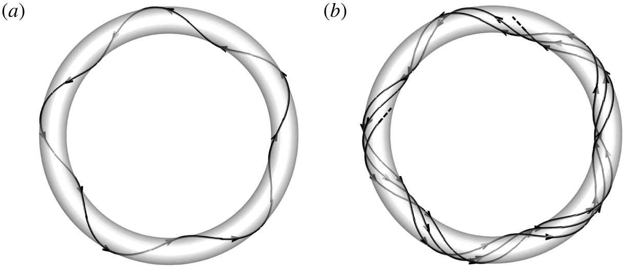
 $s=0$. As illustrated in figure 2, the field line passing through
 $(s,\unicode[STIX]{x1D70C},\unicode[STIX]{x1D703})=(0,C_{\unicode[STIX]{x1D70C}},\unicode[STIX]{x1D703}_{0})$ is on the intersection between surfaces (2.10) and (2.12).

Furthermore, the topology of twisted field lines is related to  $\unicode[STIX]{x1D6EF}(L_{C})$. As illustrated in figure 3, the field line forms a closed curve on the isosurface of
 $\unicode[STIX]{x1D70C}$ for rational
 $\unicode[STIX]{x1D6EF}(L_{C})$, and it is densely distributed for irrational
 $\unicode[STIX]{x1D6EF}(L_{C})$.
Field lines on the isosurface of  $\unicode[STIX]{x1D70C}$ with (a)
 $\unicode[STIX]{x1D6EF}(s)=5s/L_{C}$ and (b)
 $\unicode[STIX]{x1D6EF}(s)=(2+\unicode[STIX]{x03C0})s/L_{C}$.

Substituting (2.10) and (2.12) into (2.2) yields the parametric equation for field lines of  $\boldsymbol{{\mathcal{B}}}$ as
 $$\begin{eqnarray}\boldsymbol{x}(s)=\boldsymbol{c}(s)+C_{\unicode[STIX]{x1D70C}}\cos [2\unicode[STIX]{x03C0}\unicode[STIX]{x1D6EF}(s)+\unicode[STIX]{x1D703}_{0}]\boldsymbol{N}(s)+C_{\unicode[STIX]{x1D70C}}\sin [2\unicode[STIX]{x03C0}\unicode[STIX]{x1D6EF}(s)+\unicode[STIX]{x1D703}_{0}]\boldsymbol{B}(s),\end{eqnarray}$$
and the direction of  $\boldsymbol{{\mathcal{B}}}$ is
 $$\begin{eqnarray}\frac{\text{d}\boldsymbol{x}}{\text{d}s}=\frac{\text{d}\boldsymbol{c}}{\text{d}s}+C_{\unicode[STIX]{x1D70C}}\cos \unicode[STIX]{x1D703}\left(\frac{\text{d}\boldsymbol{N}}{\text{d}s}+2\unicode[STIX]{x03C0}\frac{\text{d}\unicode[STIX]{x1D6EF}}{\text{d}s}\boldsymbol{B}\right)+C_{\unicode[STIX]{x1D70C}}\sin \unicode[STIX]{x1D703}\left(\frac{\text{d}\boldsymbol{B}}{\text{d}s}-2\unicode[STIX]{x03C0}\frac{\text{d}\unicode[STIX]{x1D6EF}}{\text{d}s}\boldsymbol{N}\right).\end{eqnarray}$$
Substituting (2.1), (2.10) and (2.11) into (2.14) yields
 $$\begin{eqnarray}\frac{\text{d}\boldsymbol{x}}{\text{d}s}=(1-\unicode[STIX]{x1D705}\unicode[STIX]{x1D70C}\cos \unicode[STIX]{x1D703})\boldsymbol{e}_{s}+\unicode[STIX]{x1D70C}(\unicode[STIX]{x1D709}+\unicode[STIX]{x1D70F})\boldsymbol{e}_{\unicode[STIX]{x1D703}}.\end{eqnarray}$$
Then using (2.8) and (2.15), we obtain
 $$\begin{eqnarray}b^{\unicode[STIX]{x1D70C}}=0\end{eqnarray}$$
and
 $$\begin{eqnarray}b^{\unicode[STIX]{x1D703}}=\unicode[STIX]{x1D6E4}\frac{f\unicode[STIX]{x1D70C}}{1-\unicode[STIX]{x1D705}\unicode[STIX]{x1D70C}\cos \unicode[STIX]{x1D703}}(\unicode[STIX]{x1D709}+\unicode[STIX]{x1D70F}).\end{eqnarray}$$
Finally substituting (2.8), (2.16) and (2.17) into (2.6), we derive the vector field
 $$\begin{eqnarray}\boldsymbol{{\mathcal{B}}}=\unicode[STIX]{x1D6E4}f(\unicode[STIX]{x1D70C})\left[\boldsymbol{e}_{s}+\frac{\unicode[STIX]{x1D70C}}{1-\unicode[STIX]{x1D705}\unicode[STIX]{x1D70C}\cos \unicode[STIX]{x1D703}}(\unicode[STIX]{x1D709}+\unicode[STIX]{x1D70F})\boldsymbol{e}_{\unicode[STIX]{x1D703}}\right]\end{eqnarray}$$
for coiled and twisted flux tubes. If the tube axis is specified as a knot,  $\boldsymbol{{\mathcal{B}}}$ is knotted and is only non-trivial within the multiply connected domain
 $\unicode[STIX]{x1D6FA}_{C}$ with
 $\unicode[STIX]{x1D70C}<R_{v}$.
The axial part  $\unicode[STIX]{x1D6E4}f\boldsymbol{e}_{s}$ in equation (2.18) corresponds to the vector field with a writhe-dependent helicity (see Xiong & Yang Reference Xiong and Yang2019a), and the azimuthal part
 $\unicode[STIX]{x1D6E4}f\unicode[STIX]{x1D70C}(\unicode[STIX]{x1D709}+\unicode[STIX]{x1D70F})\boldsymbol{e}_{\unicode[STIX]{x1D703}}/(1-\unicode[STIX]{x1D705}\unicode[STIX]{x1D70C}\cos \unicode[STIX]{x1D703})$ normal to the central axis represents the twist of field lines. The twist can be tuned by varying
 $\unicode[STIX]{x1D709}$ in (2.18) and characterized by the twist helicity discussed in § 2.3.
We remark that, if the curvature of the central axis is vanishing and the azimuth of field lines in the flux tube changes at a constant rate  $\unicode[STIX]{x1D709}(s)=\unicode[STIX]{x1D6FE}$, equation (2.18) degenerates into
 $$\begin{eqnarray}\boldsymbol{{\mathcal{B}}}=\unicode[STIX]{x1D6E4}f(\unicode[STIX]{x1D70C})(\boldsymbol{e}_{s}+\unicode[STIX]{x1D70C}\unicode[STIX]{x1D6FE}\boldsymbol{e}_{\unicode[STIX]{x1D703}}),\end{eqnarray}$$
which is consistent with the form of  $\boldsymbol{{\mathcal{B}}}$ for a straight flux tube in Gold & Hoyle (Reference Gold and Hoyle1960).
As proved below, the vector field constructed by (2.18) is solenoidal, which satisfies the definition of flux tubes for magnetic or vorticity fields.
Theorem 1. The vector field  $\boldsymbol{{\mathcal{B}}}$ constructed by (2.18) is divergence-free.
Proof. From (2.1) and (2.2), the Jacobian matrix
 $$\begin{eqnarray}\unicode[STIX]{x1D645}\equiv \left(\begin{array}{@{}ccc@{}}{\displaystyle \frac{\unicode[STIX]{x2202}x}{\unicode[STIX]{x2202}s}} & {\displaystyle \frac{\unicode[STIX]{x2202}x}{\unicode[STIX]{x2202}\unicode[STIX]{x1D70C}}} & {\displaystyle \frac{\unicode[STIX]{x2202}x}{\unicode[STIX]{x2202}\unicode[STIX]{x1D703}}}\\ {\displaystyle \frac{\unicode[STIX]{x2202}y}{\unicode[STIX]{x2202}s}} & {\displaystyle \frac{\unicode[STIX]{x2202}y}{\unicode[STIX]{x2202}\unicode[STIX]{x1D70C}}} & {\displaystyle \frac{\unicode[STIX]{x2202}y}{\unicode[STIX]{x2202}\unicode[STIX]{x1D703}}}\\ {\displaystyle \frac{\unicode[STIX]{x2202}z}{\unicode[STIX]{x2202}s}} & {\displaystyle \frac{\unicode[STIX]{x2202}z}{\unicode[STIX]{x2202}\unicode[STIX]{x1D70C}}} & {\displaystyle \frac{\unicode[STIX]{x2202}z}{\unicode[STIX]{x2202}\unicode[STIX]{x1D703}}}\end{array}\right)\end{eqnarray}$$
between coordinate systems  $(s,\unicode[STIX]{x1D70C},\unicode[STIX]{x1D703})$ and
 $(x,y,z)$ is
 $$\begin{eqnarray}\unicode[STIX]{x1D645}=[(1-\unicode[STIX]{x1D705}\unicode[STIX]{x1D70C}\cos \unicode[STIX]{x1D703})\boldsymbol{T}-\unicode[STIX]{x1D70F}\unicode[STIX]{x1D70C}\sin \unicode[STIX]{x1D703}\,\boldsymbol{N}+\unicode[STIX]{x1D70F}\unicode[STIX]{x1D70C}\cos \unicode[STIX]{x1D703}\,\boldsymbol{B};\cos \unicode[STIX]{x1D703}\,\boldsymbol{N}+\sin \unicode[STIX]{x1D703}\,\boldsymbol{B};-\unicode[STIX]{x1D70C}\sin \unicode[STIX]{x1D703}\,\boldsymbol{N}+\unicode[STIX]{x1D70C}\cos \unicode[STIX]{x1D703}\,\boldsymbol{B}].\end{eqnarray}$$
Applying the inverse function theorem to (2.21), we derive
 $$\begin{eqnarray}\left.\begin{array}{@{}c@{}}\unicode[STIX]{x1D735}s={\displaystyle \frac{\boldsymbol{T}}{1-\unicode[STIX]{x1D705}\unicode[STIX]{x1D70C}\cos \unicode[STIX]{x1D703}}},\\ \unicode[STIX]{x1D735}\unicode[STIX]{x1D70C}=\cos \unicode[STIX]{x1D703}\,\boldsymbol{N}+\sin \unicode[STIX]{x1D703}\,\boldsymbol{B},\\ \unicode[STIX]{x1D735}\unicode[STIX]{x1D703}={\displaystyle \frac{-\unicode[STIX]{x1D70F}}{1-\unicode[STIX]{x1D705}\unicode[STIX]{x1D70C}\cos \unicode[STIX]{x1D703}}}\boldsymbol{T}+{\displaystyle \frac{1}{\unicode[STIX]{x1D70C}}}(-\sin \unicode[STIX]{x1D703}\,\boldsymbol{N}+\cos \unicode[STIX]{x1D703}\,\boldsymbol{B}).\end{array}\right\}\end{eqnarray}$$
Taking the divergence of (2.6) yields
 $$\begin{eqnarray}\unicode[STIX]{x1D735}\boldsymbol{\cdot }\boldsymbol{{\mathcal{B}}}=\mathop{\sum }_{i=s,\unicode[STIX]{x1D70C},\unicode[STIX]{x1D703}}\unicode[STIX]{x1D735}b^{i}\boldsymbol{\cdot }\boldsymbol{e}_{i}+b^{i}\unicode[STIX]{x1D735}\boldsymbol{\cdot }\boldsymbol{e}_{i}.\end{eqnarray}$$
Substituting (2.8), (2.16) and (2.17) into (2.23) yields
 $$\begin{eqnarray}\unicode[STIX]{x1D735}\boldsymbol{\cdot }\boldsymbol{{\mathcal{B}}}=\unicode[STIX]{x1D6E4}\left[\unicode[STIX]{x1D735}f\boldsymbol{\cdot }\boldsymbol{e}_{s}+f\unicode[STIX]{x1D735}\boldsymbol{\cdot }\boldsymbol{e}_{s}+\unicode[STIX]{x1D735}\frac{f\unicode[STIX]{x1D70C}(\unicode[STIX]{x1D709}+\unicode[STIX]{x1D70F})}{1-\unicode[STIX]{x1D705}\unicode[STIX]{x1D70C}\cos \unicode[STIX]{x1D703}}\boldsymbol{\cdot }\boldsymbol{e}_{\unicode[STIX]{x1D703}}+\frac{f\unicode[STIX]{x1D70C}(\unicode[STIX]{x1D709}+\unicode[STIX]{x1D70F})}{1-\unicode[STIX]{x1D705}\unicode[STIX]{x1D70C}\cos \unicode[STIX]{x1D703}}\unicode[STIX]{x1D735}\boldsymbol{\cdot }\boldsymbol{e}_{\unicode[STIX]{x1D703}}\right],\end{eqnarray}$$
and using (2.7) and (2.22), we have
 $$\begin{eqnarray}\unicode[STIX]{x1D735}\boldsymbol{\cdot }\boldsymbol{{\mathcal{B}}}=\unicode[STIX]{x1D6E4}\left[\unicode[STIX]{x1D735}\frac{f\unicode[STIX]{x1D70C}(\unicode[STIX]{x1D709}+\unicode[STIX]{x1D70F})}{1-\unicode[STIX]{x1D705}\unicode[STIX]{x1D70C}\cos \unicode[STIX]{x1D703}}\boldsymbol{\cdot }(-\sin \unicode[STIX]{x1D703}\,\boldsymbol{N}+\cos \unicode[STIX]{x1D703}\,\boldsymbol{B})+\frac{\unicode[STIX]{x1D705}f\unicode[STIX]{x1D70C}(\unicode[STIX]{x1D709}+\unicode[STIX]{x1D70F})\sin \unicode[STIX]{x1D703}}{(1-\unicode[STIX]{x1D705}\unicode[STIX]{x1D70C}\cos \unicode[STIX]{x1D703})^{2}}\right].\end{eqnarray}$$
Applying  $(-\sin \unicode[STIX]{x1D703}\,\boldsymbol{N}+\cos \unicode[STIX]{x1D703}\,\boldsymbol{B})\boldsymbol{\cdot }\unicode[STIX]{x1D735}s=0$ and
 $(-\sin \unicode[STIX]{x1D703}\,\boldsymbol{N}+\cos \unicode[STIX]{x1D703}\,\boldsymbol{B})\boldsymbol{\cdot }\unicode[STIX]{x1D735}\unicode[STIX]{x1D70C}=0$ to (2.25) yields
 $$\begin{eqnarray}\displaystyle & & \displaystyle \unicode[STIX]{x1D735}\frac{f\unicode[STIX]{x1D70C}(\unicode[STIX]{x1D709}+\unicode[STIX]{x1D70F})}{1-\unicode[STIX]{x1D705}\unicode[STIX]{x1D70C}\cos \unicode[STIX]{x1D703}}\boldsymbol{\cdot }(-\sin \unicode[STIX]{x1D703}\,\boldsymbol{N}+\cos \unicode[STIX]{x1D703}\,\boldsymbol{B})\nonumber\\ \displaystyle & & \displaystyle \quad =\frac{\unicode[STIX]{x2202}}{\unicode[STIX]{x2202}\unicode[STIX]{x1D703}}\left(\frac{f\unicode[STIX]{x1D70C}(\unicode[STIX]{x1D709}+\unicode[STIX]{x1D70F})}{1-\unicode[STIX]{x1D705}\unicode[STIX]{x1D70C}\cos \unicode[STIX]{x1D703}}\right)\unicode[STIX]{x1D735}\unicode[STIX]{x1D703}\boldsymbol{\cdot }(-\sin \unicode[STIX]{x1D703}\,\boldsymbol{N}+\cos \unicode[STIX]{x1D703}\,\boldsymbol{B})=-\frac{\unicode[STIX]{x1D705}f\unicode[STIX]{x1D70C}(\unicode[STIX]{x1D709}+\unicode[STIX]{x1D70F})\sin \unicode[STIX]{x1D703}}{(1-\unicode[STIX]{x1D705}\unicode[STIX]{x1D70C}\cos \unicode[STIX]{x1D703})^{2}}.\qquad\end{eqnarray}$$
Finally, substituting (2.26) into (2.25) yields  $\unicode[STIX]{x1D735}\boldsymbol{\cdot }\boldsymbol{{\mathcal{B}}}=0$.☐
In the numerical simulation of flux tubes, we usually specify (2.18) in terms of Cartesian coordinates, so we need to transform  $\boldsymbol{x}$ into
 $(s,\unicode[STIX]{x1D70C},\unicode[STIX]{x1D703})$ by (2.4) and (2.5). The numerical implementation of this transformation and the calculation of (2.18) is described in detail in appendix A. We remark that this numerical algorithm is critical for the smoothness of the constructed field and the accuracy of the helicity calculation.
2.3 Helicity
We demonstrate that the helicity of the constructed vector field  $\boldsymbol{{\mathcal{B}}}$ in (2.18) has an analytic expression distinguishing contributions from the writhe, total torsion and intrinsic twist (see Moffatt & Ricca Reference Moffatt and Ricca1992). The gauge-invariant helicity is defined as
 $$\begin{eqnarray}H\equiv \int _{\unicode[STIX]{x1D6FA}}h\,\text{d}\unicode[STIX]{x1D6FA},\end{eqnarray}$$
where  $h\equiv \boldsymbol{{\mathcal{A}}}\boldsymbol{\cdot }\boldsymbol{{\mathcal{B}}}$ is the helicity density, with the vector potential
 $\boldsymbol{{\mathcal{A}}}$ satisfying
 $\boldsymbol{{\mathcal{B}}}=\unicode[STIX]{x1D735}\times \boldsymbol{{\mathcal{A}}}$, and
 $\unicode[STIX]{x1D6FA}$ denotes the domain containing the knot. This domain is bounded by a surface with
 $\boldsymbol{{\mathcal{B}}}\boldsymbol{\cdot }\boldsymbol{n}=0$ (see Berger & Field Reference Berger and Field1984), where
 $\boldsymbol{n}$ denotes the surface normal.
For the knotted flux tubes consisting of nested toroidal magnetic surfaces, Chui & Moffatt (Reference Chui and Moffatt1995) proposed a feasible approach to derive  $H$ based on a ‘zero-framed’ coordinate system
 $$\begin{eqnarray}\left.\begin{array}{@{}c@{}}\unicode[STIX]{x1D70D}=s,\\ \unicode[STIX]{x1D712}=\unicode[STIX]{x1D719}_{v}(s,\unicode[STIX]{x1D70C},\unicode[STIX]{x1D703}),\\ \unicode[STIX]{x1D719}=\unicode[STIX]{x1D719}_{a}(s,\unicode[STIX]{x1D703}).\end{array}\right\}\end{eqnarray}$$
Here,
 $$\begin{eqnarray}\unicode[STIX]{x1D719}_{v}(s,\unicode[STIX]{x1D70C},\unicode[STIX]{x1D703})=\unicode[STIX]{x1D70C}/R_{v}\end{eqnarray}$$
is a normalized vector-surface field, whose isosurface is an integral surface of  ${\mathcal{B}}$ consisting of field lines. We remark that one of coordinates in the system of Hamada (Reference Hamada1962) or Boozer (Reference Boozer1981) also has this property of
 $\unicode[STIX]{x1D719}_{v}$. The angular variable
 $\unicode[STIX]{x1D719}_{a}(s,\unicode[STIX]{x1D703})$ in (2.28) makes the ribbon-like isosurface of
 $\unicode[STIX]{x1D719}_{a}$ ‘untwisted’. For a smooth curve
 $C$, we take
 $$\begin{eqnarray}\unicode[STIX]{x1D719}_{a}(s,\unicode[STIX]{x1D703})=\unicode[STIX]{x1D703}+\frac{2\unicode[STIX]{x03C0}{\mathcal{L}}_{S}}{L_{C}}s,\end{eqnarray}$$
where the self-linking number (see Pohl Reference Pohl1968; Moffatt & Ricca Reference Moffatt and Ricca1992)
 $$\begin{eqnarray}{\mathcal{L}}_{S}=W_{r}+T_{t}\end{eqnarray}$$
is decomposed into the writhe
 $$\begin{eqnarray}W_{r}=\frac{1}{4\unicode[STIX]{x03C0}}\oint _{C}\oint _{C}\frac{[\boldsymbol{N}(s)\times \boldsymbol{N}(s^{\prime })]\boldsymbol{\cdot }[\boldsymbol{c}(s)-\boldsymbol{c}(s^{\prime })]}{|\boldsymbol{c}(s)-\boldsymbol{c}(s^{\prime })|^{3}}\,\text{d}s\,\text{d}s^{\prime }\end{eqnarray}$$
and the normalized total torsion
 $$\begin{eqnarray}T_{t}=\frac{1}{2\unicode[STIX]{x03C0}}\oint _{C}\unicode[STIX]{x1D70F}\,\text{d}s.\end{eqnarray}$$
Substituting (2.18) into the explicit expressions of toroidal and poloidal flux functions  $T(x)$ and
 $P(x)$ in the zero-framed coordinate system (see Kruskal & Kulsrud Reference Kruskal and Kulsrud1958; Berger & Field Reference Berger and Field1984; Chui & Moffatt Reference Chui and Moffatt1995), after some algebra (see Xiong & Yang Reference Xiong and Yang2019a) we have
 $$\begin{eqnarray}\left.\begin{array}{@{}c@{}}T(x)=F(R_{v}x),\\ P(x)=[{\mathcal{L}}_{S}+\unicode[STIX]{x1D6EF}(L_{C})]F(R_{v}x),\end{array}\right\}\end{eqnarray}$$
with
 $$\begin{eqnarray}F(\unicode[STIX]{x1D70C})=2\unicode[STIX]{x03C0}\unicode[STIX]{x1D6E4}\int _{0}^{\unicode[STIX]{x1D70C}}f(\unicode[STIX]{x1D706})\unicode[STIX]{x1D706}\,\text{d}\unicode[STIX]{x1D706}.\end{eqnarray}$$
Additionally, the ‘zero-twist’ coordinate system (see Maggioni & Ricca Reference Maggioni and Ricca2009) also can be used to calculate  $T(x)$ and
 $P(x)$.
Finally, substituting (2.34) into the general expression of helicity (see Chui & Moffatt Reference Chui and Moffatt1995)
 $$\begin{eqnarray}H=2\int _{0}^{1}T(x)\frac{\text{d}P(x)}{\text{d}x}\,\text{d}x\end{eqnarray}$$
in the zero-framed coordinate system, we derive an explicit expression for the helicity decomposition
 $$\begin{eqnarray}H=\unicode[STIX]{x1D6E4}^{2}(W_{r}+T_{w}).\end{eqnarray}$$
Here, the twist
 $$\begin{eqnarray}T_{w}=T_{t}+\unicode[STIX]{x1D6EF}(L_{C})\end{eqnarray}$$
is further decomposed into the total torsion  $T_{t}$ and the intrinsic twist
 $\unicode[STIX]{x1D6EF}(L_{C})$. The geometric interpretation of the components
 $W_{r}$,
 $T_{t}$ and
 $\unicode[STIX]{x1D6EF}(L_{C})$ for a closed and self-linked ribbon is illustrated in figure 12 in Moffatt & Ricca (Reference Moffatt and Ricca1992), and these components can be computed from (2.32), (2.33) and (2.11) with given
 $\boldsymbol{c}(s)$ and
 $\unicode[STIX]{x1D709}(s)$.
Sometimes terms  $\unicode[STIX]{x1D6E4}^{2}W_{r}$ and
 $\unicode[STIX]{x1D6E4}^{2}T_{w}$ in (2.37) are referred to as the ‘centreline helicity’ and ‘twist helicity’, respectively (e.g. Scheeler et al. Reference Scheeler, Kleckner, Proment, Kindlmann and Irvine2014). In the following numerical simulation, we study the effects of the sum of
 $T_{t}$ and
 $\unicode[STIX]{x1D6EF}(L_{C})$, namely the twist helicity, on the dynamical evolution of knotted structures. In addition,
 $H$ in (2.37) for a closed tube with constant
 $P(x)/T(x)$ is consistent with an experimentally accessible form
 $H=\unicode[STIX]{x1D6E4}\oint _{C}\boldsymbol{{\mathcal{A}}}\boldsymbol{\cdot }\text{d}\boldsymbol{l}$ in Bretherton (Reference Bretherton1970) and Scheeler et al. (Reference Scheeler, van Rees, Kedia, Kleckner and Irvine2017), where
 $\text{d}\boldsymbol{l}$ denotes a line element.
As another theoretical approach, the derivations of (2.18) and (2.37) are re-expressed using Clebsch potentials in appendix B, and then the present method for constructing  $\boldsymbol{{\mathcal{B}}}$ is compared with other methods via Clebsch-like potentials in appendix C.
3 Numerical construction and simulation
3.1 Numerical construction of trefoil flux tubes
Using the method proposed in § 2, we construct trefoil flux tubes with various  $T_{w}$ from the parametric equation for
 $\boldsymbol{c}(\unicode[STIX]{x1D701})=(c_{x},c_{y},c_{z})$ as
 $$\begin{eqnarray}\left.\begin{array}{@{}c@{}}c_{x}(\unicode[STIX]{x1D701})=\unicode[STIX]{x03C0}+[1+0.5\cos (3\unicode[STIX]{x1D701})]\cos (2\unicode[STIX]{x1D701}),\\ c_{y}(\unicode[STIX]{x1D701})=\unicode[STIX]{x03C0}+[1+0.5\cos (3\unicode[STIX]{x1D701})]\sin (2\unicode[STIX]{x1D701}),\\ c_{z}(\unicode[STIX]{x1D701})=\unicode[STIX]{x03C0}-0.5\sin (2\unicode[STIX]{x1D701}).\end{array}\right\}\end{eqnarray}$$
Here,  $\unicode[STIX]{x1D701}\in [0,2\unicode[STIX]{x03C0})$ is not an arclength parameter, but it does not affect the numerical construction in appendix A.
The writhe  $W_{r}=3.52$ and the normalized total torsion
 $T_{t}=2.48$ of the curve (3.1) are calculated by (2.32) and (2.33) (see Xiong & Yang Reference Xiong and Yang2019a), respectively, and then the self-linking number
 ${\mathcal{L}}_{S}=6$ is obtained by (2.31).
In the corresponding magnetic field  $\boldsymbol{{\mathcal{B}}}$ in (2.18), we set
 $\unicode[STIX]{x1D6E4}=1$ for the strength of magnetic flux and
 $$\begin{eqnarray}f(\unicode[STIX]{x1D706})=\frac{1}{2\unicode[STIX]{x03C0}\unicode[STIX]{x1D70E}^{2}}\exp \left(-\frac{\unicode[STIX]{x1D706}^{2}}{2\unicode[STIX]{x1D70E}^{2}}\right)\end{eqnarray}$$
for the flux distribution, with  $\unicode[STIX]{x1D70E}=1/(16\sqrt{2\unicode[STIX]{x03C0}})\approx 0.025$. The radius of the flux tube is estimated as
 $R_{v}\approx 5\unicode[STIX]{x1D70E}$, and the flux tube with this small
 $R_{v}$ contains over 99.999 % of the toroidal flux in (2.18). We clip the value of
 $\boldsymbol{{\mathcal{B}}}$ outside the flux tube with
 $R_{v}$, so that
 $\boldsymbol{{\mathcal{B}}}$ can be considered as compactly supported.
We construct the trefoil flux tubes in a periodic box of sides  $L=2\unicode[STIX]{x03C0}$. This computational domain
 $\unicode[STIX]{x1D6FA}$ encloses
 $\unicode[STIX]{x1D6FA}_{C}$, and is discretized on uniform grid points
 $N^{3}$ with
 $N=512$. The solenoidal vector potential with the Coulomb gauge is calculated by the Biot–Savart law with the spectral method
 $$\begin{eqnarray}\boldsymbol{{\mathcal{A}}}={\mathcal{F}}^{-1}\left(\frac{\text{i}\boldsymbol{k}\times \widehat{\boldsymbol{{\mathcal{B}}}}}{|\boldsymbol{k}|^{2}}\right),\end{eqnarray}$$
where  ${\mathcal{F}}^{-1}$ denotes the operator of inverse Fourier transform,
 $\boldsymbol{k}$ the wavenumber in Fourier space, and
 $\widehat{\boldsymbol{{\mathcal{B}}}}={\mathcal{F}}(\boldsymbol{{\mathcal{B}}})$ the Fourier coefficient of
 $\boldsymbol{{\mathcal{B}}}$ with the Fourier transform operator
 ${\mathcal{F}}$.
We set up six cases to study the effect of twist on the evolution of magnetic knots. Since the total torsion  $T_{t}$ for the same trefoil knot (3.1) is fixed,
 $T_{w}$ in (2.38) is tuned by varying the intrinsic twist as
 $\unicode[STIX]{x1D709}=-\unicode[STIX]{x1D70F}$, 0,
 $5\times (2\unicode[STIX]{x03C0}/L_{C})$,
 $10\times (2\unicode[STIX]{x03C0}/L_{C})$,
 $20\times (2\unicode[STIX]{x03C0}/L_{C})$ and
 $30\times (2\unicode[STIX]{x03C0}/L_{C})$, with the total length
 $L_{C}=15.95$ for (3.1). We list
 $H$,
 $T_{w}$,
 $\unicode[STIX]{x1D709}$ and
 $\unicode[STIX]{x1D6EF}(L_{C})$ of the six trefoil flux tubes in table 1, and we can see that
 $H$ grows with
 $T_{w}$ in the present study, as implied from (2.37). The helicity
 $H$ is calculated by (2.27) with the numerical integration of the product of
 $\boldsymbol{{\mathcal{A}}}$ computed by (3.3) and
 $\boldsymbol{{\mathcal{B}}}$ over the periodic box. This helicity is gauge-invariant owing to the vanishing flux of
 $\boldsymbol{{\mathcal{B}}}$ across the boundary of the integral domain (see Berger & Field Reference Berger and Field1984).
Parameters and relative errors in the numerical construction of six trefoil flux tubes.

It is noted that the effects of the geometry and topology of the central axis of knotted tubes on the helicity have been investigated in Kerr (Reference Kerr2018a) and Xiong & Yang (Reference Xiong and Yang2019a). In particular, the case with  $T_{w}=0$ in table 1 corresponds to the knot construction in Xiong & Yang (Reference Xiong and Yang2019a) with
 $\boldsymbol{{\mathcal{B}}}=\unicode[STIX]{x1D6E4}f(\unicode[STIX]{x1D70C})\boldsymbol{e}_{s}$ and
 $H=\unicode[STIX]{x1D6E4}^{2}W_{r}$, where the intrinsic twist cancels out the total torsion in (2.38).
We assess the numerical construction and helicity calculation of trefoil flux tubes using (2.37). The relative numerical error in (2.37) is defined as
 $$\begin{eqnarray}\unicode[STIX]{x1D716}_{H}\equiv \frac{|H-\unicode[STIX]{x1D6E4}^{2}(W_{r}+T_{w})|}{|H|},\end{eqnarray}$$
and the negligible errors in table 1 indicate that the numerical construction is very accurate. In the numerical implementation,  $\langle |\unicode[STIX]{x1D735}\boldsymbol{\cdot }\boldsymbol{{\mathcal{B}}}|\rangle \sim O(10^{-7})$ computed from the six knotted fields are negligible, consistent with Theorem 1.
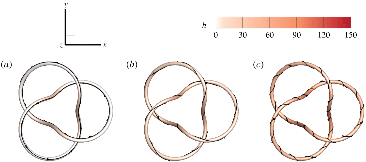
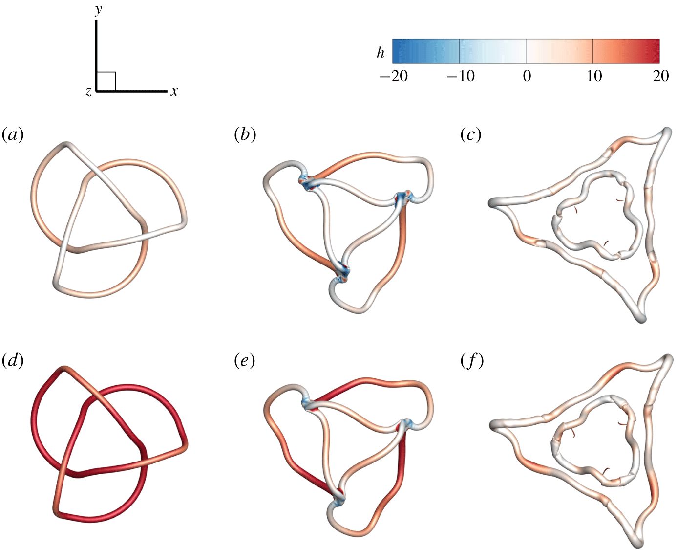
Figure 4 shows isosurfaces of  $F(\unicode[STIX]{x1D70C})=0.9$ for three typical trefoil flux tubes in table 1. We observe that the magnetic field is smooth and compact, so the constructed trefoil flux tubes are suitable for initial conditions of DNS. The isosurfaces are colour coded by the helicity density, and all the flux tubes have
 $h>0$, indicating the same chirality of
 $\boldsymbol{{\mathcal{B}}}$ and
 $\boldsymbol{{\mathcal{A}}}$. Some field lines are integrated from points on the isosurfaces, and they are on the tubes implied by (B 5).
Isosurfaces of  $F(\unicode[STIX]{x1D70C})=0.9$ of initial knotted flux tubes with (a)
 $T_{w}=0$, (b)
 $T_{w}=12.48$ and (c)
 $T_{w}=32.48$. The isosurfaces are colour coded by the helicity density. Some field lines are integrated on the surfaces.

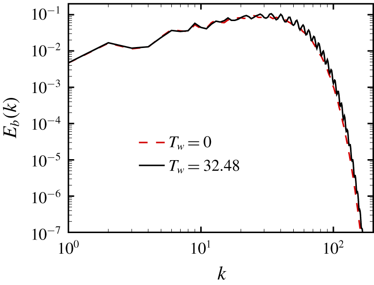
Figure 5 plots the spectrum  $E_{b}(k)$ of
 $\boldsymbol{{\mathcal{B}}}$ for the initial trefoil flux tubes. The spectrum with
 $T_{w}=0$ decays smoothly at high wavenumbers owing to the Gaussian profile
 $f(\unicode[STIX]{x1D70C})$ in (2.18) (see Melander & Hussain Reference Melander and Hussain1989; Hussain & Duraisamy Reference Hussain and Duraisamy2011; Yao & Hussain Reference Yao and Hussain2020). The spectrum with
 $T_{w}=32.48$ has slight oscillations at high wavenumbers owing to the small-scale structures generated by helical field lines surrounding the tube axis in figure 4.
Spectra of  $\boldsymbol{{\mathcal{B}}}$ for trefoil flux tubes with different
 $T_{w}$.

3.2 DNS of MHD flows
The MHD equations for an incompressible flow of constant unit density in terms of the dimensionless velocity  $\boldsymbol{u}$ and magnetic induction
 $\boldsymbol{b}$ read (e.g. Priest & Forbes Reference Priest and Forbes2000)
 $$\begin{eqnarray}\left.\begin{array}{@{}c@{}}{\displaystyle \frac{\unicode[STIX]{x2202}\boldsymbol{u}}{\unicode[STIX]{x2202}t}}+\boldsymbol{u}\boldsymbol{\cdot }\unicode[STIX]{x1D735}\boldsymbol{u}=-\unicode[STIX]{x1D735}p+\boldsymbol{j}\times \boldsymbol{b}+\unicode[STIX]{x1D708}\unicode[STIX]{x1D6FB}^{2}\boldsymbol{u},\\ {\displaystyle \frac{\unicode[STIX]{x2202}\boldsymbol{b}}{\unicode[STIX]{x2202}t}}=\unicode[STIX]{x1D735}\times (\boldsymbol{u}\times \boldsymbol{b})+\unicode[STIX]{x1D708}_{m}\unicode[STIX]{x1D6FB}^{2}\boldsymbol{b},\end{array}\right\}\end{eqnarray}$$
together with  $\unicode[STIX]{x1D735}\boldsymbol{\cdot }\boldsymbol{u}=0$ and
 $\unicode[STIX]{x1D735}\boldsymbol{\cdot }\boldsymbol{b}=0$, where
 $p$ denotes the pressure,
 $t$ the time,
 $\unicode[STIX]{x1D708}$ the kinematic viscosity,
 $\unicode[STIX]{x1D708}_{m}$ the magnetic diffusivity and
 $\boldsymbol{j}=\unicode[STIX]{x1D735}\times \boldsymbol{b}$ the current density. We set
 $\unicode[STIX]{x1D708}=\unicode[STIX]{x1D708}_{m}=0.01$. The magnetic Reynolds number is
 $Re_{m}\equiv \unicode[STIX]{x1D6E4}/\unicode[STIX]{x1D708}_{m}=100$, and the magnetic Prandtl number is
 $Pr_{m}\equiv \unicode[STIX]{x1D708}/\unicode[STIX]{x1D708}_{m}=1$.
The initial fluid is quiescent with
 $$\begin{eqnarray}\boldsymbol{u}_{0}(\boldsymbol{x})\equiv \boldsymbol{u}(\boldsymbol{x},t=0)=\mathbf{0},\end{eqnarray}$$
and the fluid motion is induced by the Lorentz force in (3.5). The initial magnetic induction is
 $$\begin{eqnarray}\boldsymbol{b}_{0}\equiv \boldsymbol{b}(\boldsymbol{x},t=0)=\boldsymbol{{\mathcal{B}}}\end{eqnarray}$$
for the trefoil flux tubes constructed in § 3.1.
The DNS of MHD flows is carried out in the periodic box  $\unicode[STIX]{x1D6FA}$ discretized on uniform grid points
 $N^{3}=512^{3}$. A symmetric form of (3.5) with Elsässer variables
 $\boldsymbol{z}^{\pm }=\boldsymbol{u}\pm \boldsymbol{b}$ (see Elsässer Reference Elsässer1950) is solved using the pseudo-spectral method (see Aluie Reference Aluie2009; Hao, Xiong & Yang Reference Hao, Xiong and Yang2019). Aliasing errors are removed using the two-thirds truncation method with the maximum wavenumber
 $k_{max}\approx N/3$. The Fourier coefficient of the velocity is advanced in time using a second-order Runge–Kutta scheme, and the time step is chosen to ensure that the Courant–Friedrichs–Lewy number is less than 0.5 for numerical stability and accuracy.
In order to ensure that the present grid can fully resolve the flow evolution, we did a convergence test by conducting another DNS with the same flow parameters on grid points  $N^{3}=1024^{3}$, and the statistics presented in § 4.1 are almost identical with those on
 $N^{3}=512^{3}$ (not shown).
4 Evolution of knotted flux tubes
4.1 Flow statistics
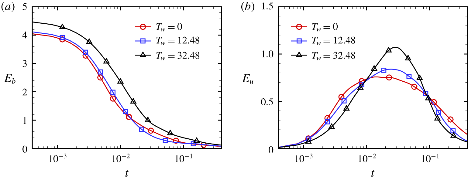
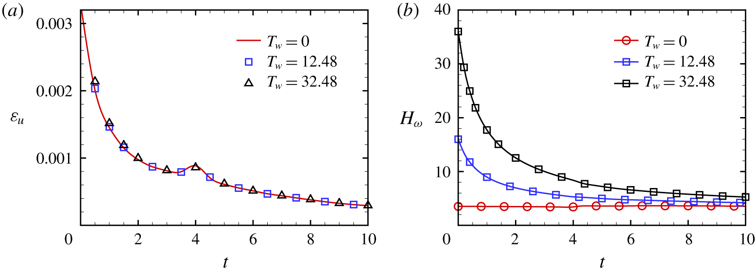
We present major flow statistics for the three typical cases  $T_{w}=0$, 12.48 and 32.48 listed in table 1. Figure 6 plots the temporal evolution of the magnetic energy
 $E_{b}=\sum _{\boldsymbol{k}}|\widehat{\boldsymbol{b}}(\boldsymbol{k})|^{2}/2$ and kinetic energy
 $E_{u}=\sum _{\boldsymbol{k}}|\widehat{\boldsymbol{u}}(\boldsymbol{k})|^{2}/2$, with Fourier coefficients
 $\widehat{\boldsymbol{b}}={\mathcal{F}}(\boldsymbol{b})$ and
 $\widehat{\boldsymbol{u}}={\mathcal{F}}(\boldsymbol{u})$. We observe that
 $E_{b}$ monotonically decays in all the cases, because a part of
 $E_{b}$ is converted into
 $E_{u}$ through the magnetic relaxation. At the mean time,
 $E_{u}$ first increases owing to the energy conversion and peaks around
 $t=0.03$. Subsequently, the system gradually becomes stable and
 $E_{u}$ decays at late times owing to the viscous dissipation, indicating the end of the relaxation process.
The temporal evolution of the (a) magnetic energy and (b) kinetic energy in the DNS of three trefoil flux tubes.

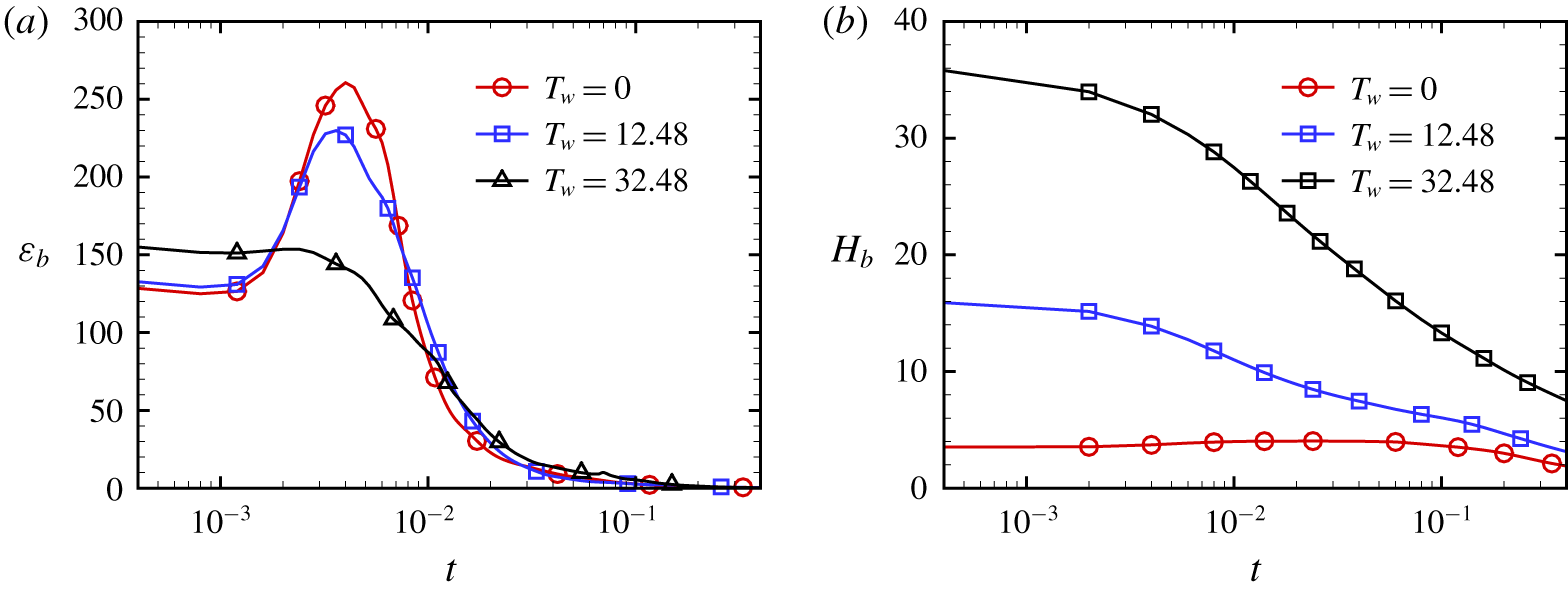
Figure 7 shows the evolution of the magnetic dissipation rate  $\unicode[STIX]{x1D700}_{b}=\unicode[STIX]{x1D708}_{m}\sum _{\boldsymbol{k}}(|\boldsymbol{k}||\widehat{\boldsymbol{b}}(\boldsymbol{k})|)^{2}$ and magnetic helicity
 $H_{b}=\int _{\unicode[STIX]{x1D6FA}}\boldsymbol{a}\boldsymbol{\cdot }\boldsymbol{b}\,\text{d}\unicode[STIX]{x1D6FA}$ with
 $\boldsymbol{a}={\mathcal{F}}^{-1}(\text{i}\boldsymbol{k}\times \widehat{\boldsymbol{b}}/|\boldsymbol{k}|^{2})$. The maximum magnetic dissipation decreases with
 $T_{w}$, and the peaks of
 $\unicode[STIX]{x1D700}_{b}$ generally coincide with the important events of topological changes of magnetic fields, which will be explained in §§ 4.2 and 4.3.
The temporal evolution of the (a) magnetic dissipation rate and (b) magnetic helicity in the DNS of three trefoil flux tubes.

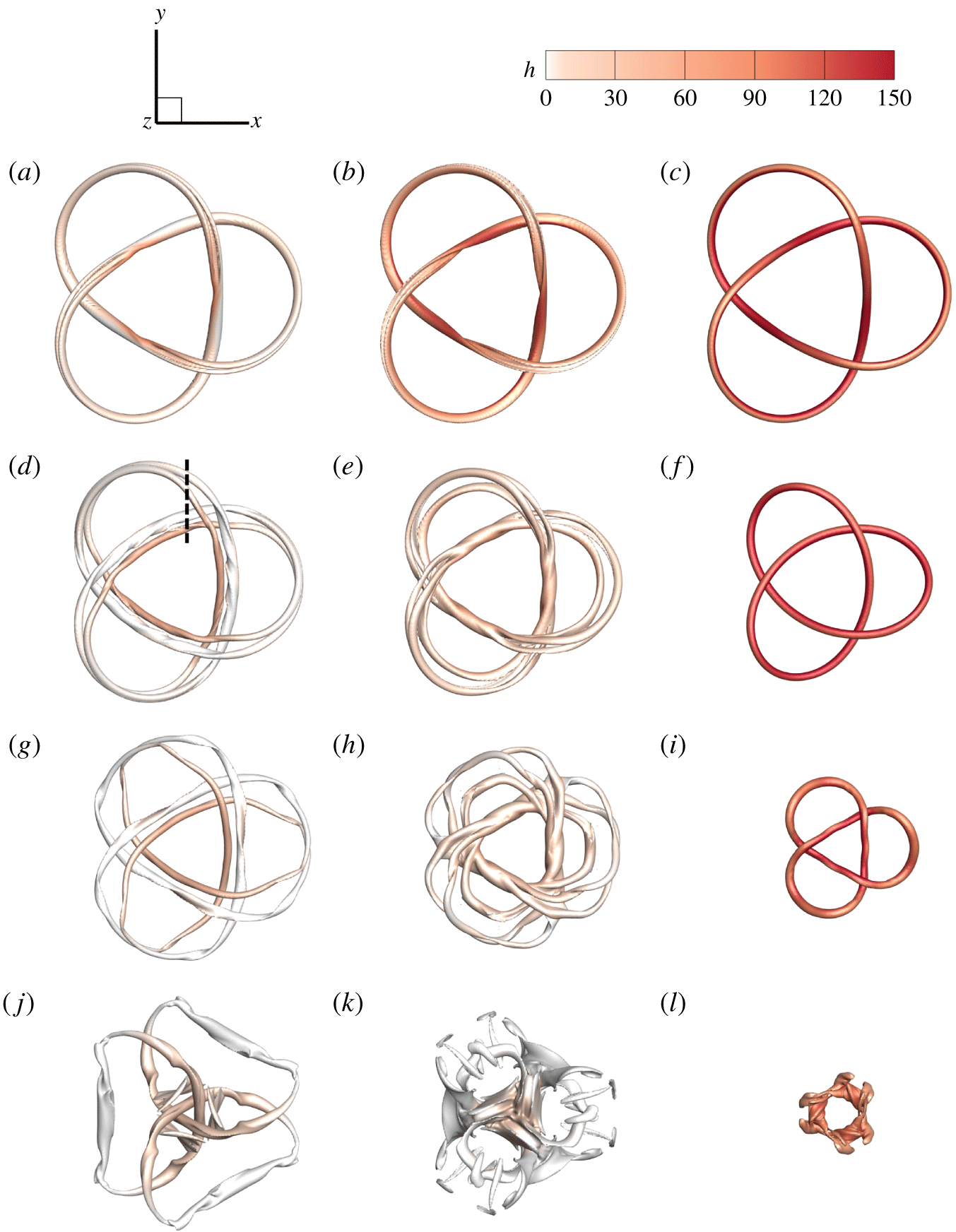
Isosurfaces of  $|\boldsymbol{b}|$ in the temporal evolution of trefoil flux tubes with
 $T_{w}=0$, 12.48 and 32.48 (columns from left to right) at
 $t=0.006$, 0.02, 0.04 and 0.1 (rows from top to bottom). All the isosurfaces are colour coded by the helicity density. The isocontour values of
 $|\boldsymbol{b}|$ are (a) 65, (b) 65, (c) 60, (d) 35, (e) 26, (f) 65, (g) 30, (h) 16, (i) 50, (j) 13, (k) 10 and (l) 33.

The evolution of  $H_{b}$ depends on the conversion between centreline and twist helicities in (2.37), and it can be non-monotonic owing to the cancellation of positive and negative
 $h$ in the integral of (2.27) (see Laing, Ricca & Sumners Reference Laing, Ricca and Sumners2015; Kerr Reference Kerr2018b). Despite the presence of dissipation effects,
 $H_{b}$ for the magnetic trefoil knot with
 $T_{w}=0$ is remarkably conserved, which is similar to the evolution of the trefoil vortex knot in viscous HD flows (see Scheeler et al. Reference Scheeler, Kleckner, Proment, Kindlmann and Irvine2014; Xiong & Yang Reference Xiong and Yang2019a). On the other hand,
 $H_{b}$ with imposed large
 $T_{w}=12.48$ and
 $32.48$ decays rapidly from the beginning.
4.2 Morphology of flux tubes
Next we discuss the relation between the major flow statistics and the morphology of the flux tubes. Under the induction of the Lorentz force, the initially quiescent flux tubes start to evolve, and their motion and morphology are significantly affected by the twisting degree  $T_{w}$ of field lines. Figure 8 depicts the evolution of isosurfaces of
 $|\boldsymbol{b}|$ colour coded by
 $h$ at
 $t=0.006$, 0.02, 0.04 and 0.1. In the early stage at
 $t\leqslant 0.02$, the magnetic knot with
 $T_{w}=0$ splits into a pair of connected trefoil flux tubes. Similarly, some parts of the knot with
 $T_{w}=12.48$ split into three offspring tubes, but some parts with high
 $h$ are still connected. By contrast, the knot with
 $T_{w}=32.48$ does not split but only shrinks, similar to the relaxation of knotted magnetic filaments in ideal MHD flows (see Moffatt Reference Moffatt1990). Therefore, the twist of field lines with large
 $T_{w}$ appears to inhibit the splitting of flux tubes.
In addition, although the cases for highly twisted flux tubes (e.g.  $T_{w}=32.48$) can exceed the threshold of the kink instability, such as the limit of Hood & Priest (Reference Hood and Priest1979), the evolution of magnetic knots is still stable owing to the numerical accuracy and symmetric configuration in our simulations without initial perturbation modes.
In figures 7(a) and 8(a,b), the occurrence of tube splitting with  $T_{w}=0$ and
 $T_{w}=12.48$ coincides with the peaks of
 $\unicode[STIX]{x1D700}_{b}$ at
 $t\approx 0.003$, consistent with the coincidence between the vortex reconnection and the peak of the dissipation rate in the evolution of vortex knots in HD flows (see Xiong & Yang Reference Xiong and Yang2019a). For large
 $T_{w}=32.48$,
 $\unicode[STIX]{x1D700}_{b}$ of the knot without tube splitting in figure 8(c) has no obvious peak.
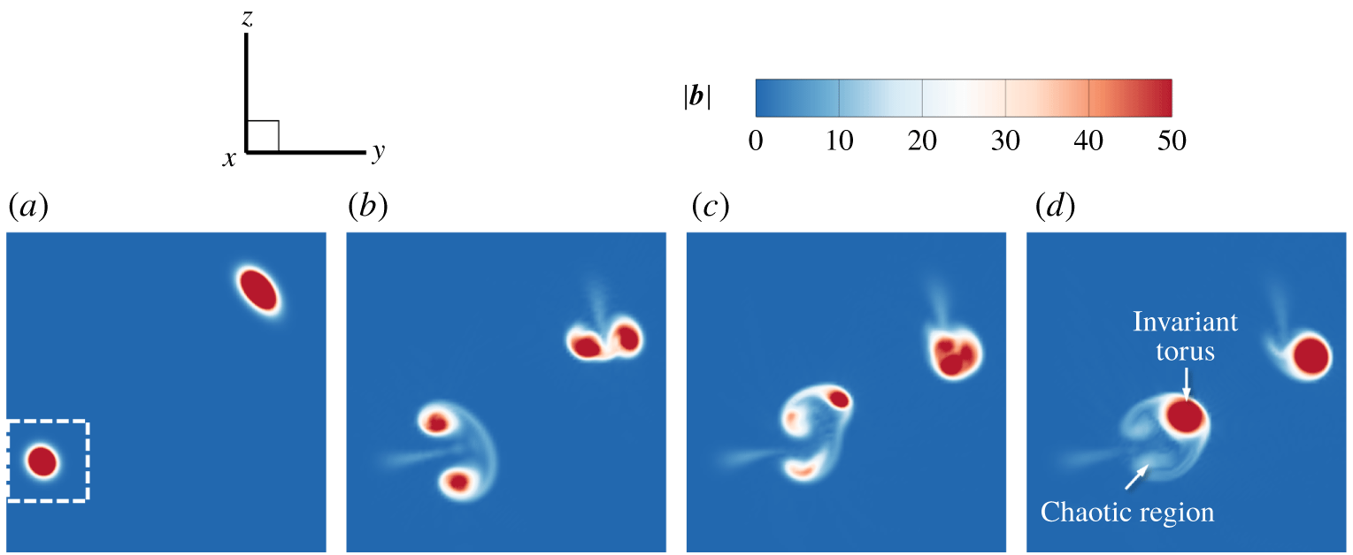
Figure 9 plots plane cuts of the contour of  $|\boldsymbol{b}|$ at
 $x=\unicode[STIX]{x03C0}$. At
 $t=0$, the contour for
 $T_{w}=0$ in figure 9(a) is almost identical to those for other
 $T_{w}$. At
 $t=0.02$, two cross-sections of each flux tube at
 $t=0$ tend to approach to each other for all the cases, implying shrinking of the knots. In cases
 $T_{w}=0$ and 12.48, each cross-section splits into two and three parts with concentrated
 $|\boldsymbol{b}|$, respectively. In case
 $T_{w}=32.48$, the cross-section of
 $|\boldsymbol{b}|$ does not split, consistent with the observation in figure 8.
Plane cuts of the contour of  $|\boldsymbol{b}|$ at
 $x=\unicode[STIX]{x03C0}$: (a)
 $T_{w}=0$ at
 $t=0$; (b)
 $T_{w}=0$ at
 $t=0.02$; (c)
 $T_{w}=12.48$ at
 $t=0.02$; and (d)
 $T_{w}=32.48$ at
 $t=0.02$. The range of the contours is marked by the dashed line in figure 8(d).

At a later time  $t=0.04$, separations of the split flux tubes with
 $T_{w}=0$ and
 $T_{w}=12.48$ are more notable, whereas the tube with
 $T_{w}=32.48$ remains the initial topology. Finally, at
 $t=0.1$, both
 $E_{b}$ and
 $E_{u}$ are low in figure 6, so dissipation processes with finite
 $\unicode[STIX]{x1D708}_{m}$ and
 $\unicode[STIX]{x1D708}$ dominate. The isosurfaces of
 $|\boldsymbol{b}|$ for all the cases deviate from flux tubes and their geometry becomes more complex.
We remark that the morphology of the isosurface of  $|\boldsymbol{b}|$ can be different from that of field lines (see Xiong & Yang Reference Xiong and Yang2019b), and next we will discuss the detailed dynamics of field lines inside flux tubes.
4.3 Effects of twist on the splitting of flux tubes
We elucidate how the flux tubes split under the Lorentz force  $\boldsymbol{f}_{L}\equiv \boldsymbol{j}\times \boldsymbol{b}$. Since
 $\boldsymbol{u}$ is very small at early times, we rewrite the momentum equation in (3.5) with only the leading-order terms of
 $\boldsymbol{u}$ as
 $$\begin{eqnarray}\frac{\unicode[STIX]{x2202}\boldsymbol{u}}{\unicode[STIX]{x2202}t}-\unicode[STIX]{x1D708}\unicode[STIX]{x1D6FB}^{2}\boldsymbol{u}=\boldsymbol{f}_{L}-\unicode[STIX]{x1D735}p.\end{eqnarray}$$
Taking the divergence of (4.1) for the incompressible flow, we have
 $$\begin{eqnarray}\unicode[STIX]{x1D735}\boldsymbol{\cdot }(\,\boldsymbol{f}_{L}-\unicode[STIX]{x1D735}p)=0.\end{eqnarray}$$
Thus the force exerted on flux tubes can be interpreted as a projection of  $\boldsymbol{f}_{L}$ onto divergence-free space.
The Lorentz force after the divergence-free projection can be expressed as
 $$\begin{eqnarray}\boldsymbol{f}_{p}\equiv \boldsymbol{f}_{L}-\unicode[STIX]{x1D735}\unicode[STIX]{x1D6F7},\end{eqnarray}$$
with  $\unicode[STIX]{x1D6F7}=\unicode[STIX]{x0394}^{-1}\boldsymbol{f}_{L}$. In the numerical implementation,
 $\boldsymbol{f}_{p}$ is calculated by
 $$\begin{eqnarray}\boldsymbol{f}_{p}=\boldsymbol{f}_{L}-{\mathcal{F}}^{-1}\left(\frac{\widehat{\boldsymbol{f}}_{L}\boldsymbol{\cdot }\boldsymbol{k}}{|\boldsymbol{k}|^{2}}\boldsymbol{k}\right),\end{eqnarray}$$
with  $\widehat{\boldsymbol{f}}_{L}={\mathcal{F}}(\,\boldsymbol{f}_{L})$.
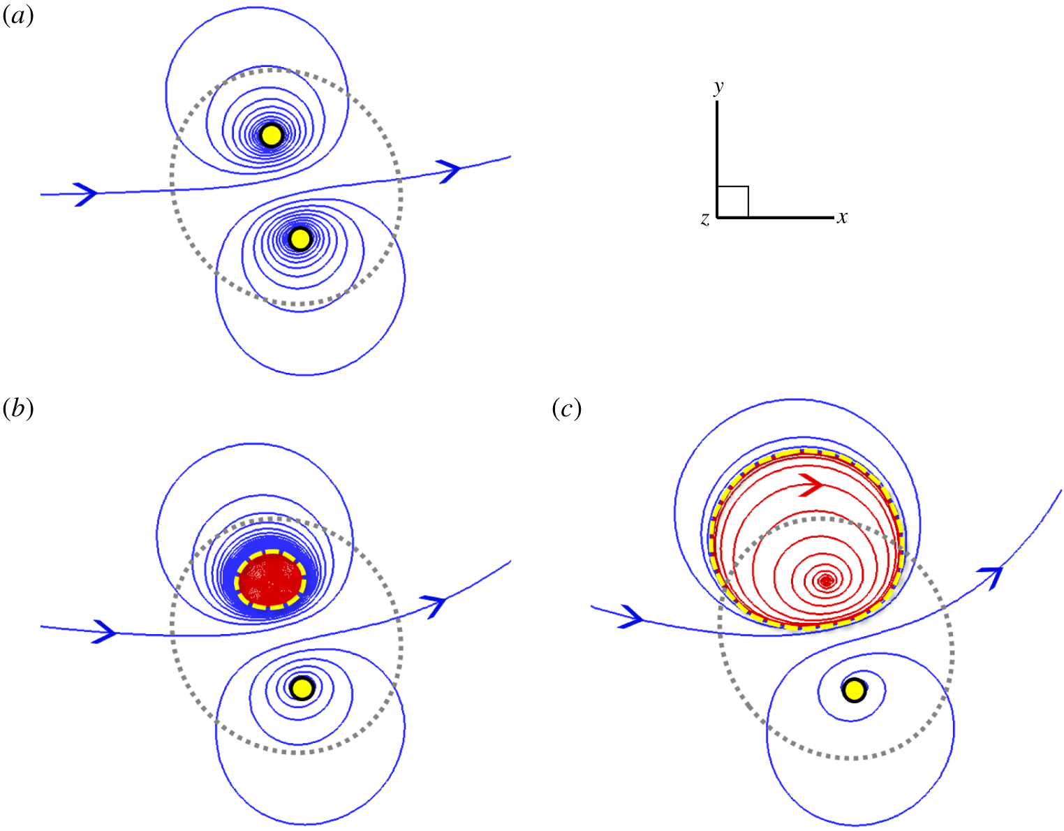
Figure 10 plots the projection of integral lines of  $\boldsymbol{f}_{p}$ on the plane at
 $x=\unicode[STIX]{x03C0}$ for the three magnetic knots at
 $t=0$. These force lines for
 $T_{w}=0$ form a counter-rotating, dipole-like pattern and drive a bundle of field lines inside the flux tube to split into two, also shown as the splitting tubes in figures 8(d) and 9(b).
Projection of the integral lines of  $\boldsymbol{f}_{p}$ onto the plane at
 $x=\unicode[STIX]{x03C0}$ for three magnetic knots with (a)
 $T_{w}=0$, (b)
 $T_{w}=12.48$ and (c)
 $T_{w}=32.48$ at
 $t=0$. The range of each panel is marked by the dotted box in figure 9(a). The grey dotted circle denotes the isosurface of
 $|\boldsymbol{b}|=5\,\%\,|\boldsymbol{b}|_{max}$, as the boundary of flux tubes. The yellow circle and the dashed curve, respectively, denote the spiral point and the limit cycle in the phase portrait for
 $\boldsymbol{f}_{p}$.

We find that  $T_{w}$ has an impact on the phase portrait for the nonlinear characteristic equation of
 $\boldsymbol{f}_{L}$. Figure 10(a) for
 $T_{w}=0$ shows stable and unstable spiral points at the dipole centres on the phase plane at
 $x=\unicode[STIX]{x03C0}$, and the two critical points have nearly mirror symmetry. For
 $T_{w}>0$, the stable spiral point becomes a limit cycle in figure 10(b), and this Hopf bifurcation breaks the mirror symmetry of
 $\boldsymbol{f}_{p}$ in the phase portrait. Furthermore, the area of the limit cycle grows with
 $T_{w}$ in figure 10(c).
Implied from figures 9 and 10, the limit cycle appears to move faster than the stable spiral point and carry the major potion of high-intensity field lines in the evolution of flux tubes. The structural transition with  $T_{w}$ in the phase portrait corresponds to the morphology of splitting/unsplitting flux tubes in figure 8(d–f).
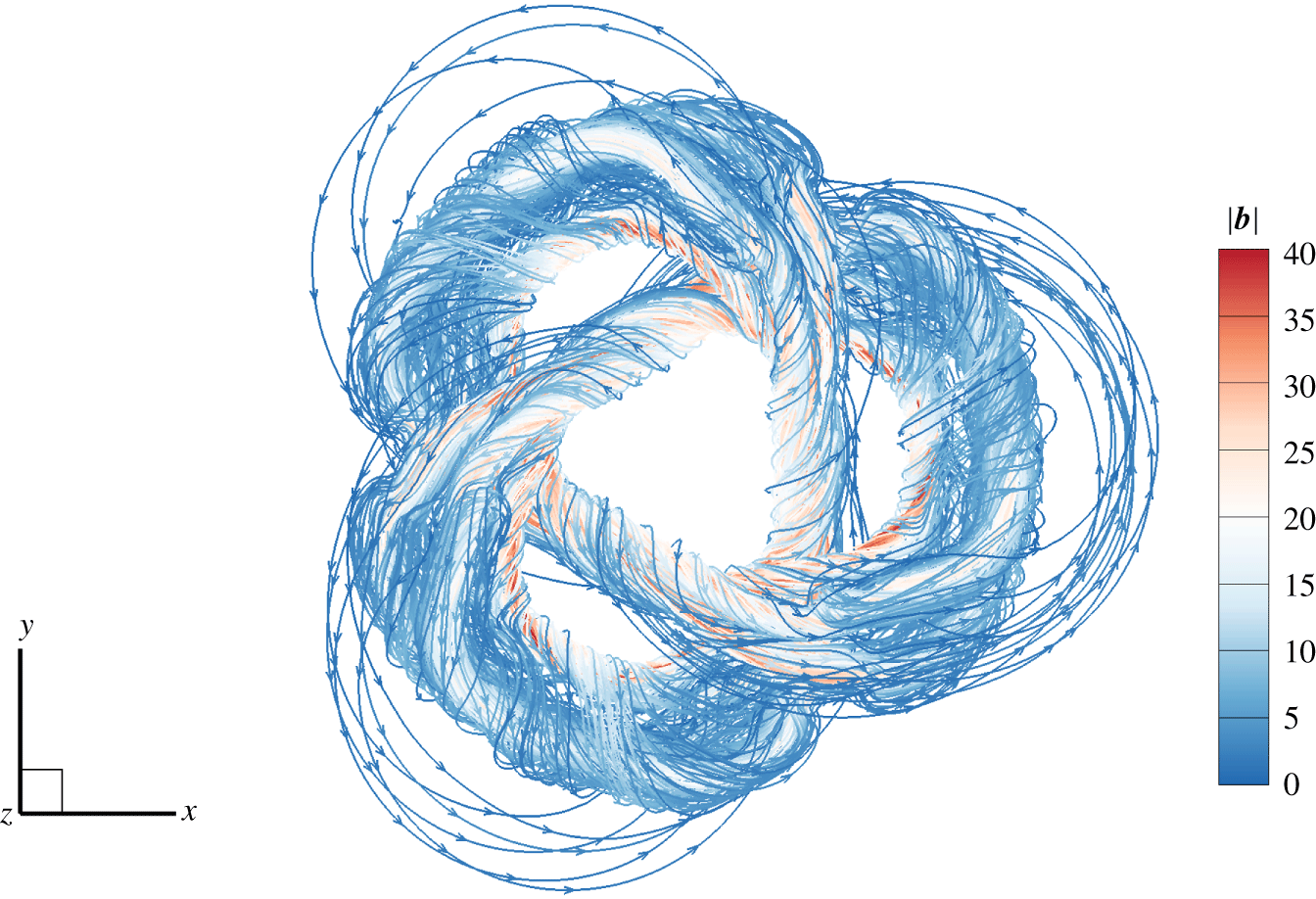
Inside the flux tube, the spiral  $\boldsymbol{f}_{L}$ can drive the initially parallel field lines into chaotic ones. For example, figure 11 depicts a highly chaotic and braided field line for the knot with
 $T_{w}=12.48$ at
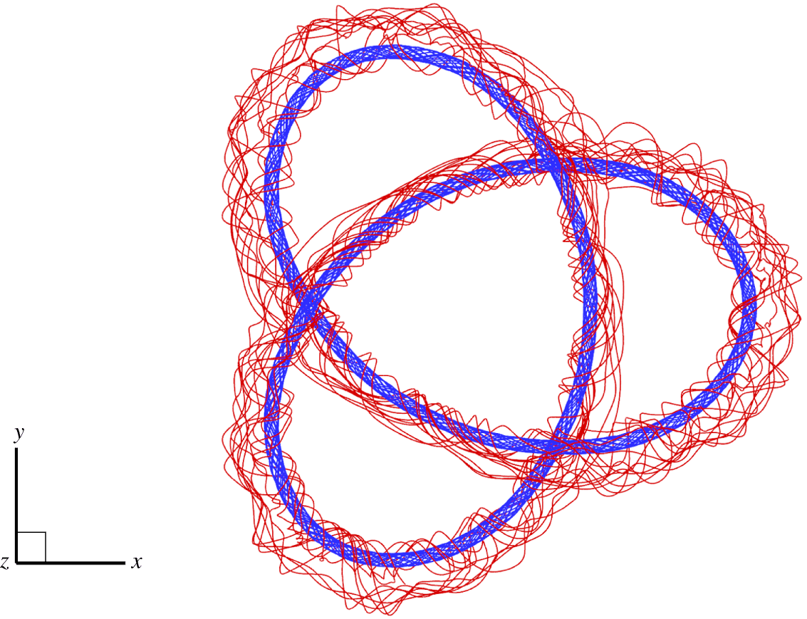
 $t=0.04$, and the chaos of field lines can be further quantified (see Smiet et al. Reference Smiet, Candelaresi, Thompson, Swearngin, Dalhuisen and Bouwmeester2015). On the other hand, the field lines inside the limit cycle are very stable without chaos. Figure 12 depicts the coexistence of an inner invariant torus and an outer chaotic field line. Considering that field lines at high
 $Re_{m}$ move with the fluid from the Alfvén theorem, the mechanism for the transition to chaos is similar to the chaotic mixing for passive scalars (see Aref Reference Aref1984).
A chaotic field line colour coded by  $|\boldsymbol{b}|$ for the magnetic knot with
 $T_{w}=12.48$ at
 $t=0.04$.

An inner field line (blue) on an invariant torus and an outer field line (red) in the chaotic region for the magnetic knot with  $T_{w}=32.48$ at
 $t=0.04$.

The splitting of flux tubes and the chaotic rearrangement of field lines for  $T_{w}=0$ and
 $T_{w}=12.48$ contribute to the rise of
 $\unicode[STIX]{x1D700}_{b}$ in figure 7(a) and the relatively low peaks of
 $E_{u}$ in figure 6(b). Therefore, increasing
 $T_{w}$ can achieve more stable field lines and less energy loss in the relaxation of flux tubes, which could be useful for the design of tokamaks (see Strauss Reference Strauss1976; Wesson Reference Wesson1976; Wingen et al. Reference Wingen, Wilcox, Seal, Unterberg, Cianciosa, Delgado-Aparicio, Hirshman and Lao1976).
Moreover, in contrast to the significant influence of  $T_{w}$ on the evolution of magnetic knots, the twist with varying
 $\unicode[STIX]{x1D709}$ in table 1 has negligible effects on the evolution of vortex knots in HD flows, which is discussed in appendix D.
5 Conclusions
We develop a general method for constructing knotted flux tubes with finite thickness, arbitrary shape and tunable twist. From the parametric equation of a given smooth and non-degenerate closed curve, we construct a vector field based on a curved cylindrical coordinate system along the curve. The vector has axial and azimuthal components. The axial component is determined by a given kernel function, which decays with the radial distance from the curve. The azimuthal component is derived from our proposed constraints. We prove that this vector field is strictly divergence-free, so it can be used as the initial field of a magnetic/vortex tube whose central axis is prescribed by the curve.
Within the framework of Chui & Moffatt (Reference Chui and Moffatt1995), we derive the expression of  $H$ for the constructed vector field. This helicity can be explicitly decomposed into writhe, normalized total torsion and intrinsic twist, so we can isolate the effect of each component in the investigation of helicity.
Corresponding to the theoretical construction, we extend the algorithm in Xiong & Yang (Reference Xiong and Yang2019a) to construct knotted flux tubes with tunable twist in Cartesian coordinates. The relative numerical errors in the helicity calculation of trefoil flux tubes with a range of  $T_{w}$ from 0 to 32.48 are negligible in a periodic box.
We use the constructed vector fields as initial magnetic inductions in DNS, and calculate the evolution of trefoil magnetic flux tubes with various  $T_{w}$ in resistive MHD flows. We find that
 $T_{w}$ has an impact on the evolution of magnetic knots. For large
 $T_{w}$, the magnetic knot gradually shrinks to a tight stable state, similar to the relaxation process in ideal MHD flows. For small
 $T_{w}$, the knotted flux tube splits and reconnects at early times, accompanied by the drastic release of the magnetic energy.
The effect of twist on the tube splitting is elucidated by the phase portrait of the Lorentz force projected onto the divergence-free space. The initial counter-rotating  $\boldsymbol{f}_{p}$ drives a bundle of field lines inside the flux tube into two for
 $T_{w}=0$. With increasing
 $T_{w}$, an unstable spiral point of
 $\boldsymbol{f}_{p}$ becomes a limit cycle via the Hopf bifurcation. The field lines inside the limit cycle form invariant tori, whereas the field lines outside the limit cycle become chaotic. The split of flux tubes and the chaotic rearrangement of field lines for low
 $T_{w}$ lead to the rise of the magnetic dissipation rate.
In future work, the proposed method can be used to construct vortex/magnetic tubes in highly complex configurations. Furthermore, we expect to carry out a detailed, quantitative study (e.g. Moffatt Reference Moffatt2014; Laing et al. Reference Laing, Ricca and Sumners2015) to elucidate the conversion between writhe and twist in the helicity evolution.
Acknowledgements
Numerical simulations were carried out on the TH-2A supercomputer in Guangzhou, PR China. This work has been supported in part by the National Natural Science Foundation of China (grant nos 11925201, 91952108 and 91841302).
Declaration of interests
The authors report no conflict of interest.
Appendix A. Numerical algorithm for computing $\boldsymbol{{\mathcal{B}}}$

We construct a solenoidal  $\boldsymbol{{\mathcal{B}}}$ for a flux tube surrounding the central axis described by a given characteristic equation. The coil of the flux tube is determined by the central axis, and the local twist is determined by the helical component
 $b^{\unicode[STIX]{x1D703}}$ in (2.18) around the central axis. The algorithm for computing
 $\boldsymbol{{\mathcal{B}}}$ in (2.18) is an extension of that in Xiong & Yang (Reference Xiong and Yang2019a) by incorporating the tunable twist. The idea behind the algorithm is that, for a given
 $\boldsymbol{x}$ and a parametric curve
 $C\boldsymbol{ : }\boldsymbol{c}(\unicode[STIX]{x1D701})$, we seek all the stationary points of
 $|\boldsymbol{x}-\boldsymbol{c}(\unicode[STIX]{x1D701})|$ as a set
 $$\begin{eqnarray}S_{\unicode[STIX]{x1D701}}(\boldsymbol{x})=\{\unicode[STIX]{x1D701}\mid (\boldsymbol{x}-\boldsymbol{c}(\unicode[STIX]{x1D701}))\boldsymbol{\cdot }\boldsymbol{T}(\unicode[STIX]{x1D701})=0\}.\end{eqnarray}$$
Here, it is not necessary for  $\unicode[STIX]{x1D701}$ to be an arclength parameter (see Xiong & Yang Reference Xiong and Yang2019a).
For each  $\unicode[STIX]{x1D701}\in S_{\unicode[STIX]{x1D701}}$, the corresponding pole distance and azimuthal coordinate in the plane
 $S_{C}$ normal to curve
 $C$ are
 $$\begin{eqnarray}\unicode[STIX]{x1D70C}_{\unicode[STIX]{x1D701}}=|\boldsymbol{x}-\boldsymbol{c}(\unicode[STIX]{x1D701})|\end{eqnarray}$$
and
 $$\begin{eqnarray}\unicode[STIX]{x1D703}_{\unicode[STIX]{x1D701}}=\arccos \frac{[\boldsymbol{x}-\boldsymbol{c}(\unicode[STIX]{x1D701})]\boldsymbol{\cdot }\boldsymbol{N}(\unicode[STIX]{x1D701})}{\unicode[STIX]{x1D70C}_{\unicode[STIX]{x1D701}}},\end{eqnarray}$$
respectively. Then (2.18) is calculated as
 $$\begin{eqnarray}\boldsymbol{{\mathcal{B}}}(\boldsymbol{x})=\mathop{\sum }_{\unicode[STIX]{x1D701}\in S_{\unicode[STIX]{x1D701}}(\boldsymbol{x})}\boldsymbol{{\mathcal{B}}}_{\unicode[STIX]{x1D701}},\end{eqnarray}$$
where  $\boldsymbol{{\mathcal{B}}}_{\unicode[STIX]{x1D701}}$ is calculated by substituting
 $(\unicode[STIX]{x1D701},\unicode[STIX]{x1D70C}_{\unicode[STIX]{x1D701}},\unicode[STIX]{x1D703}_{\unicode[STIX]{x1D701}})$ into (2.18). Note that one
 $\boldsymbol{x}$ may correspond to multiple
 $\unicode[STIX]{x1D701}$ in
 $S_{\unicode[STIX]{x1D701}}(\boldsymbol{x})$, but only one
 $\unicode[STIX]{x1D701}$ with
 $\unicode[STIX]{x1D70C}_{\unicode[STIX]{x1D701}}<R_{v}$ contributes to the summation in (A 4) via the non-trivial kernel function
 $f(\unicode[STIX]{x1D70C}_{\unicode[STIX]{x1D701}})$ defined in (2.9). We remark that, if
 $R_{v}$ is too large, the constructed flux tube may self-intersect, corresponding to multiple non-vanishing terms in (A 4), and we can still compute a smooth vector field by (A 4) (see Xiong & Yang Reference Xiong and Yang2019a).
Next we give technical details for computing (A 4) with the discretization of  $C$. For a given, closed parametric curve
 $C\boldsymbol{ : }\boldsymbol{c}(\unicode[STIX]{x1D701})$ with
 $\unicode[STIX]{x1D701}\in [0,L_{\unicode[STIX]{x1D701}})$, we divide
 $C$ into
 $N_{C}$ segments by
 $N_{C}$ dividing points
 $$\begin{eqnarray}\boldsymbol{c}_{i}=\boldsymbol{c}(\unicode[STIX]{x1D701}_{i}),\quad i=1,2,\ldots ,N_{C},\end{eqnarray}$$
with  $\unicode[STIX]{x1D701}_{i}=(i-1)\unicode[STIX]{x0394}\unicode[STIX]{x1D701}$ and
 $\unicode[STIX]{x0394}\unicode[STIX]{x1D701}=L_{\unicode[STIX]{x1D701}}/N_{C}$. If
 $N_{C}$ is large enough, curve
 $C$ can be approximated as a fold line connecting all the dividing points. Then the space in the proximity of curve
 $C$ can be divided into
 $N_{C}$ subdomains,
 $$\begin{eqnarray}\unicode[STIX]{x1D6FA}_{i}=\{\boldsymbol{x}\mid (\boldsymbol{x}-\boldsymbol{c}_{i})\boldsymbol{\cdot }\boldsymbol{T}_{i}\geqslant 0\text{ and }(\boldsymbol{x}-\boldsymbol{c}_{i+1})\boldsymbol{\cdot }\boldsymbol{T}_{i+1}<0\},\end{eqnarray}$$
with
 $$\begin{eqnarray}\boldsymbol{T}_{i}=\frac{\boldsymbol{c}_{i+1}-\boldsymbol{c}_{i}}{|\boldsymbol{c}_{i+1}-\boldsymbol{c}_{i}|},\quad i=1,2,\ldots ,N_{C},\end{eqnarray}$$
where subscripts  $N_{C}+1$ and 1 are equivalent.
For a given  $\boldsymbol{x}$, we first use (A 6) to determine the subdomains
 $\unicode[STIX]{x1D6FA}_{i}$ containing
 $\boldsymbol{x}$. The subscripts of all the
 $\unicode[STIX]{x1D6FA}_{i}$ containing
 $\boldsymbol{x}$ are denoted by a set
 $$\begin{eqnarray}\widetilde{I}_{\unicode[STIX]{x1D701}}(\boldsymbol{x})=\{j\mid \boldsymbol{x}\in \unicode[STIX]{x1D6FA}_{j}\}.\end{eqnarray}$$
For each  $j\in \widetilde{I}_{\unicode[STIX]{x1D701}}(\boldsymbol{x})$, the parameter of curve
 $C$ is approximated by
 $$\begin{eqnarray}\widetilde{\unicode[STIX]{x1D701}}_{j}=\frac{\unicode[STIX]{x1D701}_{j+1}(\boldsymbol{x}-\boldsymbol{c}_{j})\boldsymbol{\cdot }\boldsymbol{T}_{j}+\unicode[STIX]{x1D701}_{j}(\boldsymbol{c}_{j+1}-\boldsymbol{x})\boldsymbol{\cdot }\boldsymbol{T}_{j}}{|\boldsymbol{c}_{j+1}-\boldsymbol{c}_{j}|},\end{eqnarray}$$
and the discretized point set of  $\unicode[STIX]{x1D701}$ for (A 1) is collected by
 $$\begin{eqnarray}S_{\unicode[STIX]{x1D701}}(\boldsymbol{x})=\{\widetilde{\unicode[STIX]{x1D701}}_{j}\mid j\in \widetilde{I}_{\unicode[STIX]{x1D701}}(\boldsymbol{x})\}.\end{eqnarray}$$
At  $\widetilde{\boldsymbol{c}}_{j}=\boldsymbol{c}(\widetilde{\unicode[STIX]{x1D701}}_{j})$, we use the second-order finite difference scheme to calculate the Frenet–Serret frame
 $$\begin{eqnarray}\left.\begin{array}{@{}c@{}}\widetilde{\boldsymbol{T}}_{j}=\boldsymbol{T}(\widetilde{\unicode[STIX]{x1D701}}_{j}),\\ \widetilde{\boldsymbol{N}}_{j}=\boldsymbol{N}(\widetilde{\unicode[STIX]{x1D701}}_{j}),\\ \widetilde{\boldsymbol{B}}_{j}=\boldsymbol{B}(\widetilde{\unicode[STIX]{x1D701}}_{j}),\end{array}\right\}\end{eqnarray}$$
as well as the curvature, torsion and the rate of change  $\unicode[STIX]{x1D709}$ of the azimuth in (2.18) as
 $$\begin{eqnarray}\left.\begin{array}{@{}c@{}}\widetilde{\unicode[STIX]{x1D705}}_{j}=\unicode[STIX]{x1D705}(\widetilde{\unicode[STIX]{x1D701}}_{j}),\\ \widetilde{\unicode[STIX]{x1D70F}}_{j}=\unicode[STIX]{x1D70F}(\widetilde{\unicode[STIX]{x1D701}}_{j}),\\ \widetilde{\unicode[STIX]{x1D709}}_{j}=\unicode[STIX]{x1D709}(\widetilde{\unicode[STIX]{x1D701}}_{j}).\end{array}\right\}\end{eqnarray}$$
In addition, the distance from  $\boldsymbol{c}(\widetilde{\unicode[STIX]{x1D701}}_{j})$ is calculated by
 $$\begin{eqnarray}\widetilde{\unicode[STIX]{x1D70C}}_{j}=|\boldsymbol{x}-\widetilde{c}_{j}|,\end{eqnarray}$$
and azimuth-related functions are calculated by
 $$\begin{eqnarray}\left.\begin{array}{@{}c@{}}\cos \widetilde{\unicode[STIX]{x1D703}}_{j}={\displaystyle \frac{(\boldsymbol{x}-\widetilde{c}_{j})\boldsymbol{\cdot }\widetilde{\boldsymbol{N}}_{j}}{\widetilde{\unicode[STIX]{x1D70C}}_{j}}},\\ \sin \widetilde{\unicode[STIX]{x1D703}}_{j}={\displaystyle \frac{(\boldsymbol{x}-\widetilde{c}_{j})\boldsymbol{\cdot }\widetilde{\boldsymbol{B}}_{j}}{\widetilde{\unicode[STIX]{x1D70C}}_{j}}}.\end{array}\right\}\end{eqnarray}$$
Finally, we approximate equation (A 4) as
 $$\begin{eqnarray}\boldsymbol{{\mathcal{B}}}(\boldsymbol{x})=\mathop{\sum }_{j\in \widetilde{I}_{\unicode[STIX]{x1D701}}(\boldsymbol{x})}\widetilde{\boldsymbol{{\mathcal{B}}}}_{j},\end{eqnarray}$$
with
 $$\begin{eqnarray}\widetilde{\boldsymbol{{\mathcal{B}}}}_{j}=\left\{\begin{array}{@{}ll@{}}\unicode[STIX]{x1D6E4}f(\widetilde{\unicode[STIX]{x1D70C}}_{j})\left[\widetilde{\boldsymbol{T}}_{j}+{\displaystyle \frac{\widetilde{\unicode[STIX]{x1D70C}}_{j}(\widetilde{\unicode[STIX]{x1D709}}_{j}+\widetilde{\unicode[STIX]{x1D70F}}_{j})}{1-\widetilde{\unicode[STIX]{x1D705}}_{j}\widetilde{\unicode[STIX]{x1D70C}}_{j}\cos \widetilde{\unicode[STIX]{x1D703}}_{j}}}(-\sin \widetilde{\unicode[STIX]{x1D703}}_{j}\,\widetilde{\boldsymbol{N}}_{j}+\cos \widetilde{\unicode[STIX]{x1D703}}_{j}\,\widetilde{\boldsymbol{B}}_{j})\right],\quad & 1>\widetilde{\unicode[STIX]{x1D705}}_{j}\widetilde{\unicode[STIX]{x1D70C}}_{j}\cos \widetilde{\unicode[STIX]{x1D703}}_{j},\\ \mathbf{0},\quad & 1\leqslant \widetilde{\unicode[STIX]{x1D705}}_{j}\widetilde{\unicode[STIX]{x1D70C}}_{j}\cos \widetilde{\unicode[STIX]{x1D703}}_{j}.\end{array}\right.\end{eqnarray}$$
The procedure for the numerical construction of  $\boldsymbol{{\mathcal{B}}}(\boldsymbol{x})$ is summarized in algorithm 1.

Appendix B. Construction of knotted fields using Clebsch potentials
We provide another perspective for the derivation of the knotted field (2.18) and its helicity (2.37) via Clebsch potentials (Clebsch Reference Clebsch1859). This reformulation gives a geometric interpretation of (2.18), and is useful for comparing our method to some existing ones (see appendix C).
A solenoidal vector field
 $$\begin{eqnarray}\boldsymbol{{\mathcal{B}}}=\unicode[STIX]{x1D735}F\times \unicode[STIX]{x1D735}G,\end{eqnarray}$$
except for  $\boldsymbol{{\mathcal{B}}}=0$ (see Graham & Henyey Reference Graham and Henyey2000), can be locally expressed by a pair of Clebsch potentials
 $F$ and
 $G$. Given
 $\boldsymbol{{\mathcal{B}}}$ in (2.18) and
 $F$ in (2.35), we derive
 $$\begin{eqnarray}G=-\int _{\unicode[STIX]{x1D6E4}_{\unicode[STIX]{x1D70C}}}\frac{\unicode[STIX]{x1D73B}\times \boldsymbol{{\mathcal{B}}}\boldsymbol{\cdot }\text{d}\boldsymbol{x}}{\unicode[STIX]{x1D73B}\boldsymbol{\cdot }\unicode[STIX]{x1D735}F}\end{eqnarray}$$
from (11.5) in Truesdell (Reference Truesdell1954), where  $\unicode[STIX]{x1D73B}$ is a continuous vector field with
 $\unicode[STIX]{x1D73B}\boldsymbol{\cdot }\unicode[STIX]{x1D735}F\neq 0$, and
 $\unicode[STIX]{x1D6E4}_{\unicode[STIX]{x1D70C}}$ is the integration path lying on an isosurface of
 $F$. Setting
 $\unicode[STIX]{x1D73B}=\unicode[STIX]{x1D701}^{s}\boldsymbol{e}_{s}+\unicode[STIX]{x1D701}^{\unicode[STIX]{x1D70C}}\boldsymbol{e}_{\unicode[STIX]{x1D70C}}+\unicode[STIX]{x1D701}^{\unicode[STIX]{x1D703}}\boldsymbol{e}_{\unicode[STIX]{x1D703}}$ with
 $\unicode[STIX]{x1D701}^{\unicode[STIX]{x1D70C}}\neq 0$, and substituting it into (B 2) yields
 $$\begin{eqnarray}G=\int _{\unicode[STIX]{x1D6E4}_{\unicode[STIX]{x1D70C}}}\frac{\text{d}\unicode[STIX]{x1D703}}{2\unicode[STIX]{x03C0}}-\,\text{d}\unicode[STIX]{x1D6EF}.\end{eqnarray}$$
A particular (B 3) can be
 $$\begin{eqnarray}G=\frac{\unicode[STIX]{x1D703}}{2\unicode[STIX]{x03C0}}-\unicode[STIX]{x1D6EF}(s).\end{eqnarray}$$
Thus the intersection of isosurfaces of  $F$ and
 $G$ represents the field line (see figure 2), and each isosurface consists of field lines, e.g.
 $$\begin{eqnarray}\boldsymbol{{\mathcal{B}}}\boldsymbol{\cdot }\unicode[STIX]{x1D735}F(\unicode[STIX]{x1D70C})=0.\end{eqnarray}$$
The representations of Clebsch potentials and vector-surface fields are useful for flow diagnostics (e.g. Yang & Pullin Reference Yang and Pullin2010) and visualization (e.g. Chern et al. Reference Chern, Knöppel, Pinkall and Schröder2017).
Using (B 1), the vector potential can be expressed as
 $$\begin{eqnarray}\boldsymbol{{\mathcal{A}}}=F\unicode[STIX]{x1D735}G+\unicode[STIX]{x1D735}\unicode[STIX]{x1D6F9},\end{eqnarray}$$
where  $\unicode[STIX]{x1D6F9}$ is a multi-valued function defined in
 $\unicode[STIX]{x1D6FA}_{C}$ (see Rosner et al. Reference Rosner, Low, Tsinganos and Berger1989). We remark that, although
 $G$ and
 $\unicode[STIX]{x1D6F9}$ are multi-valued functions,
 $F\unicode[STIX]{x1D735}G$ and
 $\unicode[STIX]{x1D735}\unicode[STIX]{x1D6F9}$ are single-valued smooth ones in
 $\unicode[STIX]{x1D6FA}_{C}$, so (B 1) and (B 6) are still smooth in
 $\unicode[STIX]{x1D6FA}_{C}$.
Substituting (B 6) into (2.27) and using  $F\unicode[STIX]{x1D735}G\boldsymbol{\cdot }\boldsymbol{{\mathcal{B}}}=0$ from (B 1) yields
 $$\begin{eqnarray}H=\int _{\unicode[STIX]{x1D6FA}_{C}}\unicode[STIX]{x1D735}\unicode[STIX]{x1D6F9}\boldsymbol{\cdot }\boldsymbol{{\mathcal{B}}}\,\text{d}\unicode[STIX]{x1D6FA}=\int _{\unicode[STIX]{x1D6FA}_{C}}\unicode[STIX]{x1D735}\boldsymbol{\cdot }(\unicode[STIX]{x1D6F9}\boldsymbol{{\mathcal{B}}})\,\text{d}\unicode[STIX]{x1D6FA}.\end{eqnarray}$$
Applying the divergence theorem to (B 7) in the multiply connected domain  $\unicode[STIX]{x1D6FA}_{C}$ for a knotted tube, we have
 $$\begin{eqnarray}H=\int _{\unicode[STIX]{x2202}\unicode[STIX]{x1D6FA}_{C}}\unicode[STIX]{x1D6F9}\boldsymbol{{\mathcal{B}}}\boldsymbol{\cdot }\boldsymbol{n}\,\text{d}S+\int _{S_{c}}\unicode[STIX]{x1D6FF}\unicode[STIX]{x1D6F9}\boldsymbol{{\mathcal{B}}}\boldsymbol{\cdot }\boldsymbol{n}\,\text{d}S,\end{eqnarray}$$
where  $S_{c}$ is a cross-section cutting the tube at
 $s=\text{const.}$ with
 $(\unicode[STIX]{x1D70C},\unicode[STIX]{x1D703})\in [0,1]\times [0,2\unicode[STIX]{x03C0})$, and
 $\unicode[STIX]{x1D6FF}\unicode[STIX]{x1D6F9}$ denotes the difference of
 $\unicode[STIX]{x1D6F9}$ on the two sides of
 $S_{c}$. Considering
 $\boldsymbol{{\mathcal{B}}}=\mathbf{0}$ on the boundary
 $\unicode[STIX]{x2202}\unicode[STIX]{x1D6FA}_{C}$ for the field compactly supported in
 $\unicode[STIX]{x1D6FA}_{C}$, (B 8) becomes
 $$\begin{eqnarray}H=\int _{S_{c}}\unicode[STIX]{x1D6FF}\unicode[STIX]{x1D6F9}\boldsymbol{{\mathcal{B}}}\boldsymbol{\cdot }\boldsymbol{n}\,\text{d}S.\end{eqnarray}$$
In general,  $\unicode[STIX]{x1D6FF}\unicode[STIX]{x1D6F9}$ depends on the gauge
 $\unicode[STIX]{x1D6F9}$, but an arbitrary
 $\unicode[STIX]{x1D6F9}$ may prevent
 $\boldsymbol{{\mathcal{A}}}$ in (B 6) from smoothly extending to a simply connected region
 $\unicode[STIX]{x1D6FA}$ containing
 $\unicode[STIX]{x1D6FA}_{C}$. Thus we impose a restriction on
 $\unicode[STIX]{x1D6F9}$ so that
 $\boldsymbol{{\mathcal{A}}}$ can be smoothly extended to
 $\unicode[STIX]{x1D6FA}$ and the extended
 $\boldsymbol{{\mathcal{A}}}$ (still denoted as
 $\boldsymbol{{\mathcal{A}}}$) is curl-free outside
 $\unicode[STIX]{x1D6FA}_{C}$. Then we will prove that
 $\unicode[STIX]{x1D6FF}\unicode[STIX]{x1D6F9}$ is independent of
 $\unicode[STIX]{x1D6F9}$, i.e. the helicity calculated by (B 9) is gauge-invariant.
We derive  $\unicode[STIX]{x1D6FF}\unicode[STIX]{x1D6F9}$ at
 $\boldsymbol{x}=(\unicode[STIX]{x1D70D}_{x},\unicode[STIX]{x1D712}_{x},\unicode[STIX]{x1D719}_{x})$ in
 $\unicode[STIX]{x1D6FA}_{C}$ using the zero-framed coordinate system defined in (2.28). First,
 $\unicode[STIX]{x1D735}\unicode[STIX]{x1D6F9}=\boldsymbol{{\mathcal{A}}}-F\unicode[STIX]{x1D735}G$ from (B 6) is integrated along path
 $\unicode[STIX]{x1D6E4}_{\unicode[STIX]{x1D719}}=\{(\unicode[STIX]{x1D70D},\unicode[STIX]{x1D712},\unicode[STIX]{x1D719})\mid \unicode[STIX]{x1D70D}\in [0,L_{C}],~\unicode[STIX]{x1D712}=\unicode[STIX]{x1D712}_{x},~\unicode[STIX]{x1D719}=\unicode[STIX]{x1D719}_{x}\}$ (see Xiong & Yang Reference Xiong and Yang2019a) as
 $$\begin{eqnarray}\unicode[STIX]{x1D6FF}\unicode[STIX]{x1D6F9}(\boldsymbol{x})=\oint _{\unicode[STIX]{x1D6E4}_{\unicode[STIX]{x1D719}}}\boldsymbol{{\mathcal{A}}}\boldsymbol{\cdot }\text{d}\boldsymbol{l}-\oint _{\unicode[STIX]{x1D6E4}_{\unicode[STIX]{x1D719}}}F\unicode[STIX]{x1D735}G\boldsymbol{\cdot }\text{d}\boldsymbol{l}.\end{eqnarray}$$
Applying the Stokes theorem to the first term on the right-hand side of (B 10) yields
 $$\begin{eqnarray}\oint _{\unicode[STIX]{x1D6E4}_{\unicode[STIX]{x1D719}}}\boldsymbol{{\mathcal{A}}}\boldsymbol{\cdot }\text{d}\boldsymbol{l}=\int _{S_{\unicode[STIX]{x1D719}}}\boldsymbol{{\mathcal{B}}}\boldsymbol{\cdot }\boldsymbol{n}\,\text{d}S,\end{eqnarray}$$
where  $S_{\unicode[STIX]{x1D719}}$ is a surface spanned by
 $\unicode[STIX]{x1D6E4}_{\unicode[STIX]{x1D719}}$, e.g. the Seifert surface. Since
 $\boldsymbol{{\mathcal{B}}}$ vanishes outside
 $\unicode[STIX]{x1D6FA}_{C}$, we take
 $S_{\unicode[STIX]{x1D719}}=R_{\unicode[STIX]{x1D719}}(1)\setminus R_{\unicode[STIX]{x1D719}}(\unicode[STIX]{x1D712}_{x})$, the set difference of
 $R_{\unicode[STIX]{x1D719}}(1)$ and
 $R_{\unicode[STIX]{x1D719}}(\unicode[STIX]{x1D712}_{x})$, where
 $R_{\unicode[STIX]{x1D719}}(\unicode[STIX]{x1D712}_{x})$ denotes a ribbon at
 $\unicode[STIX]{x1D719}=\unicode[STIX]{x1D719}_{x}$ with
 $(\unicode[STIX]{x1D70D},\unicode[STIX]{x1D712})\in [0,L_{C})\times [0,\unicode[STIX]{x1D712}_{x}]$ (see Xiong & Yang Reference Xiong and Yang2019a). Thus (B 11) becomes
 $$\begin{eqnarray}\int _{R_{\unicode[STIX]{x1D719}}(1)}\boldsymbol{{\mathcal{B}}}\boldsymbol{\cdot }\boldsymbol{n}\,\text{d}S-\int _{R_{\unicode[STIX]{x1D719}}(\unicode[STIX]{x1D712}_{x})}\boldsymbol{{\mathcal{B}}}\boldsymbol{\cdot }\boldsymbol{n}\,\text{d}S=P(1)-P(\unicode[STIX]{x1D712}_{x}),\end{eqnarray}$$
where the definition of the poloidal flux function  $P(\unicode[STIX]{x1D712}_{x})$ in Xiong & Yang (Reference Xiong and Yang2019a) is used. Substituting (B 4) into the second term on the right-hand side of (B 10) and using (2.29), (2.30) and (2.34) yields
 $$\begin{eqnarray}\oint _{\unicode[STIX]{x1D6E4}_{\unicode[STIX]{x1D719}}}F\unicode[STIX]{x1D735}G\boldsymbol{\cdot }\text{d}\boldsymbol{l}=-F(R_{v}\unicode[STIX]{x1D712}_{x})[{\mathcal{L}}_{S}+\unicode[STIX]{x1D6EF}(L_{C})]=-P(\unicode[STIX]{x1D712}_{x}).\end{eqnarray}$$
Then substituting (B 12) and (B 13) into (B 10) and using (2.9), (2.34), (2.31) and (2.38), we obtain that
 $$\begin{eqnarray}\unicode[STIX]{x1D6FF}\unicode[STIX]{x1D6F9}=P(1)=\unicode[STIX]{x1D6E4}[{\mathcal{L}}_{S}+\unicode[STIX]{x1D6EF}(L_{C})]=\unicode[STIX]{x1D6E4}(W_{r}+T_{w})\end{eqnarray}$$
is a constant in  $\unicode[STIX]{x1D6FA}_{C}$ for a given
 $\boldsymbol{{\mathcal{B}}}$, which implies that the helicity calculated by (B 9) is gauge-invariant. Finally, substituting (B 14) into (B 9) yields
 $$\begin{eqnarray}H=\unicode[STIX]{x1D6E4}(W_{r}+T_{w})\int _{S_{c}}\boldsymbol{{\mathcal{B}}}\boldsymbol{\cdot }\boldsymbol{n}\,\text{d}S=\unicode[STIX]{x1D6E4}^{2}(W_{r}+T_{w}),\end{eqnarray}$$
where  $\int _{S_{c}}\boldsymbol{{\mathcal{B}}}\boldsymbol{\cdot }\boldsymbol{n}\,\text{d}S=\unicode[STIX]{x1D6E4}$ is the toroidal flux strength through
 $S_{c}$. Therefore, the helicity expressions (2.37) and (B 15) are identical.
We remark that the knotted field  $\boldsymbol{{\mathcal{B}}}$ in (2.18) with
 $H\neq 0$ is represented by a Clebsch potential pair (2.35) and (B 4) in the multiply connected domain
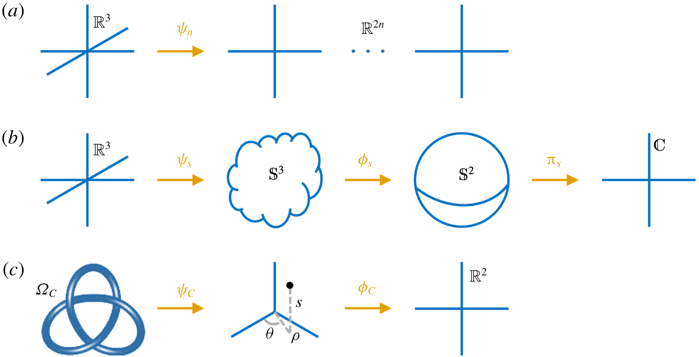
 $\unicode[STIX]{x1D6FA}_{C}$, where (B 4) is a multi-valued function. If the Clebsch potentials are restricted to be globally smooth and single-valued, multiple Clebsch pairs (see Zakharov & Kuznetsov Reference Zakharov and Kuznetsov1997; Cartes et al. Reference Cartes, Bustamante and Brachet2007) or spherical Clebsch maps (see Chern et al. Reference Chern, Knöppel, Pinkall and Schröder2017) are required for representing a knotted field with
 $H\neq 0$, which is further discussed in appendix C.
Schematic comparison of the maps for transforming a solenoidal vector field into Clebsch-like potentials: (a)  $n$-dimensional Clebsch map, (b) spherical Clebsch map and (c) the present method.

Appendix C. Construction methods via Clebsch-like maps
Besides the present Clebsch map in (B 1), there are several existing ones for constructing vector fields that are related to Clebsch potentials. The basic idea is to transform a vector field into Clebsch-like potentials using various mappings, as sketched in figure 13 and elaborated below. Next we briefly review these methods and then stress the advantages of our proposed method.
C.1 The $n$-dimensional Clebsch map

The original potentials of Clebsch (Reference Clebsch1859) cannot globally represent knotted fields with non-vanishing helicity (see He & Yang Reference He and Yang2016) and may not exist near points with  $\boldsymbol{{\mathcal{B}}}=\mathbf{0}$ (see Graham & Henyey Reference Graham and Henyey2000). A natural generalization (see Zakharov & Kuznetsov Reference Zakharov and Kuznetsov1997; Cartes et al. Reference Cartes, Bustamante and Brachet2007) uses
 $n$-dimensional functions
 $\unicode[STIX]{x1D74D}_{n}=(\unicode[STIX]{x1D736},\unicode[STIX]{x1D737}):\unicode[STIX]{x211D}^{3}\rightarrow \unicode[STIX]{x211D}^{2n}$,
 $n\geqslant 1$,
 $\unicode[STIX]{x1D736}=(\unicode[STIX]{x1D6FC}_{1},\ldots ,\unicode[STIX]{x1D6FC}_{n})$,
 $\unicode[STIX]{x1D737}=(\unicode[STIX]{x1D6FD}_{1},\ldots ,\unicode[STIX]{x1D6FD}_{n})$, to construct a vector field
 $$\begin{eqnarray}\boldsymbol{{\mathcal{B}}}=\mathop{\sum }_{i=1}^{n}\unicode[STIX]{x1D735}\unicode[STIX]{x1D6FC}_{i}\times \unicode[STIX]{x1D735}\unicode[STIX]{x1D6FD}_{i},\end{eqnarray}$$
with non-vanishing helicity. On the other hand, this generalized Clebsch presentation (with  $n\geqslant 2$) contains less geometric information than the original one in the form of (B 1), because field lines and vector surfaces cannot be presented by isosurfaces of these scalar functions.
C.2 Spherical Clebsch map
This type of method involves the mapping between spherical domains (see Chern et al. Reference Chern, Knöppel, Pinkall and Schröder2017). Based on the mapping of Hopf (Reference Hopf1931), Kamchatnov (Reference Kamchatnov1982) proposed a special magnetic configuration consisting of closed field lines for describing topological solitons in MHD flows. In the construction of the magnetic field, a three-dimensional sphere  $\unicode[STIX]{x1D54A}^{3}$ is first embedded into a four-dimensional Euclidean space. Then the connection between
 $\unicode[STIX]{x1D54A}^{3}$ and
 $\unicode[STIX]{x211D}^{3}$ is established by the inverse transformation of a stereographic projection
 $\unicode[STIX]{x1D74D}_{s}:\unicode[STIX]{x211D}^{3}\rightarrow \unicode[STIX]{x1D54A}^{3}$, and the three-dimensional sphere
 $\unicode[STIX]{x1D54A}^{3}$ is further transformed into a two-dimensional sphere
 $\unicode[STIX]{x1D54A}^{2}=\{(s_{1},s_{2},s_{3})\mid s_{1}^{2}+s_{2}^{2}+s_{3}^{2}=1\}$ by the Hopf mapping
 $\unicode[STIX]{x1D753}_{s}\boldsymbol{ : }\unicode[STIX]{x1D54A}^{3}\rightarrow \unicode[STIX]{x1D54A}^{2}$. From mappings
 $\unicode[STIX]{x1D74D}_{s}$ and
 $\unicode[STIX]{x1D753}_{s}$, Kamchatnov (Reference Kamchatnov1982) obtained
 $$\begin{eqnarray}\boldsymbol{{\mathcal{B}}}=\frac{1}{4\unicode[STIX]{x03C0}}(s_{1}\unicode[STIX]{x1D735}s_{2}\times \unicode[STIX]{x1D735}s_{3}+s_{2}\unicode[STIX]{x1D735}s_{3}\times \unicode[STIX]{x1D735}s_{1}+s_{3}\unicode[STIX]{x1D735}s_{1}\times \unicode[STIX]{x1D735}s_{2}).\end{eqnarray}$$
By projecting  $\unicode[STIX]{x1D54A}^{2}$ onto a complex plane
 $\unicode[STIX]{x2102}$ with the stereographic projection
 $\unicode[STIX]{x1D745}_{s}\boldsymbol{ : }\unicode[STIX]{x1D54A}^{2}\rightarrow \unicode[STIX]{x2102}=\{\unicode[STIX]{x1D753}=\unicode[STIX]{x1D719}_{r}+\text{i}\unicode[STIX]{x1D719}_{i}\mid \unicode[STIX]{x1D719}_{r},\unicode[STIX]{x1D719}_{i}\in \unicode[STIX]{x211D}\}$ with
 $$\begin{eqnarray}\unicode[STIX]{x1D719}_{r}=\frac{s_{1}}{1-s_{3}}\quad \text{and}\quad \unicode[STIX]{x1D719}_{i}=\frac{s_{2}}{1-s_{3}},\end{eqnarray}$$
equation (C 2) can be expressed in terms of Clebsch potentials as (see Ranada Reference Ranada1989)
 $$\begin{eqnarray}\boldsymbol{{\mathcal{B}}}=\unicode[STIX]{x1D735}\left(\frac{1}{4\unicode[STIX]{x03C0}\text{i}}\log \frac{\unicode[STIX]{x1D753}}{\unicode[STIX]{x1D753}^{\ast }}\right)\times \unicode[STIX]{x1D735}\left(\frac{\unicode[STIX]{x1D753}\unicode[STIX]{x1D753}^{\ast }}{1+\unicode[STIX]{x1D753}\unicode[STIX]{x1D753}^{\ast }}\right).\end{eqnarray}$$
This field can be knotted with non-vanishing helicity due to the singularity of  $\log (\unicode[STIX]{x1D753}/\unicode[STIX]{x1D753}^{\ast })/(4\unicode[STIX]{x03C0}\text{i})$.
Several recent studies adapted Kamchatnov’s approach to the numerical construction of knotted flux tubes. Chern et al. (Reference Chern, Knöppel, Pinkall, Schröder and Weissmann2016, Reference Chern, Knöppel, Pinkall and Schröder2017) developed a numerical algorithm for reconstructing mapping  $\unicode[STIX]{x1D74D}_{s}$, but in principle the constructed field can only have quantized helicity. Other similar methods, such as rational mappings (see Kedia et al. Reference Kedia, Foster, Dennis and Irvine2016) and exponential mappings (see Smiet et al. Reference Smiet, Candelaresi, Thompson, Swearngin, Dalhuisen and Bouwmeester2015, Reference Smiet, Candelaresi and Bouwmeester2017), modify mappings
 $\unicode[STIX]{x1D753}_{s}$ and
 $\unicode[STIX]{x1D745}_{s}$. A major issue of the methods via spherical Clebsch maps is the lack of a general method for constructing scalar potentials.
C.3 The present method
In the present study, the entire Euclidean space  $\unicode[STIX]{x211D}^{3}$ is divided into a compactly supported tubular domain and a null one. In the closed tube
 $\unicode[STIX]{x1D6FA}_{C}$, equations (2.4) and (2.5) can be viewed as a mapping
 $\unicode[STIX]{x1D74D}_{C}:\unicode[STIX]{x1D6FA}_{C}\rightarrow C_{C}$ of
 $\unicode[STIX]{x1D6FA}_{C}$ in Cartesian coordinates to a cylinder
 $C_{C}$ in
 $(s,\unicode[STIX]{x1D70C},\unicode[STIX]{x1D703})$ with
 $0\leqslant s<L_{C}$ and
 $\unicode[STIX]{x1D70C}<R_{v}$. Subsequently, the cylinder is mapped to a two-dimensional Euclidean space by
 $\unicode[STIX]{x1D753}_{C}:C_{C}\rightarrow \unicode[STIX]{x211D}^{2}$ with scalar functions
 $F$ in (2.35) and
 $G$ in (B 4). Thus the Clebsch presentation (B 1) is obtained through the two maps sketched in figure 13(c). It is noted that the tubular domain
 $\unicode[STIX]{x1D6FA}_{C}$ is multiply connected, so the corresponding
 $\boldsymbol{{\mathcal{B}}}$ can have non-vanishing helicity, e.g. (B 15).
Furthermore, for rational  $\unicode[STIX]{x1D6EF}(L_{C})$ in (2.11) (see figure 3a), we link (B 1) and (C 2) by setting
 $\unicode[STIX]{x1D6EF}(L_{C})=p/q$ with co-prime integers
 $(p,q)$ and
 $$\begin{eqnarray}\left.\begin{array}{@{}c@{}}s_{1}=2\sqrt{{\displaystyle \frac{F}{\unicode[STIX]{x1D6E4}}}\left(1-{\displaystyle \frac{F}{\unicode[STIX]{x1D6E4}}}\right)}\cos (2\unicode[STIX]{x03C0}qG),\\ s_{2}=2\sqrt{{\displaystyle \frac{F}{\unicode[STIX]{x1D6E4}}}\left(1-{\displaystyle \frac{F}{\unicode[STIX]{x1D6E4}}}\right)}\sin (2\unicode[STIX]{x03C0}qG),\\ s_{3}=1-2{\displaystyle \frac{F}{\unicode[STIX]{x1D6E4}}},\end{array}\right\}\end{eqnarray}$$
so that (B 1) can be expressed in the form of (C 2) as
 $$\begin{eqnarray}\boldsymbol{{\mathcal{B}}}=\frac{\unicode[STIX]{x1D6E4}}{4\unicode[STIX]{x03C0}q}(s_{1}\unicode[STIX]{x1D735}s_{2}\times \unicode[STIX]{x1D735}s_{3}+s_{2}\unicode[STIX]{x1D735}s_{3}\times \unicode[STIX]{x1D735}s_{1}+s_{3}\unicode[STIX]{x1D735}s_{1}\times \unicode[STIX]{x1D735}s_{2}),\end{eqnarray}$$
with globally smooth, single-valued functions  $s_{1}$,
 $s_{2}$ and
 $s_{3}$. For irrational
 $\unicode[STIX]{x1D6EF}(L_{C})$ (see figure 3b), the discontinuous field
 $(s_{1},s_{2},s_{3})$ in (C 5) in
 $\unicode[STIX]{x211D}^{3}$ cannot be used to define a continuous field from (C 6), which implies that (B 1) is more generalized than (C 6) for constructing twisted flux tubes.
Compared with existing methods, our method has the following advantages:
(i) The knotted flux tube is characterized by a given parametric equation instead of multiple scalar functions, which is more feasible than the methods relying on tailored scalar potentials in the forms of (C 1) and (C 4).
(ii) The helicity of flux tubes can have any value, instead of the restrictions to the vanishing helicity in the original Clebsch presentation or quantized helicity in (C 4).
(iii) The components of helicity, i.e. the writhe, normalized total torsion and intrinsic twist, have analytic expressions.
(iv) The strength of the flux tube is specified by a compactly supported smooth function, and the radius of the tube is constant, which facilitate the numerical simulation of the flux tube on uniform grid points.
Appendix D. Evolution of trefoil vortex tubes in viscous HD flows
In order to show the effect of twist on different fluid systems, we show the evolution of trefoil vortex tubes in viscous HD flows with various  $T_{w}$ and
 $\boldsymbol{b}_{0}=\mathbf{0}$. The DNS solver is the same as that in § 3.2.
The vorticity field  $\unicode[STIX]{x1D74E}$ at
 $t=0$ is set to
 $\boldsymbol{{\mathcal{B}}}$ for three trefoil vortex tubes with
 $T_{w}=0$, 12.48 and 32.48. The isosurfaces of initial
 $|\unicode[STIX]{x1D74E}|$ are the same as those in figure 4. The initial velocity field for (3.5) is solved by the Biot–Savart law. In the present DNS of HD flows, we take
 $\unicode[STIX]{x1D708}=0.0004$, and the Reynolds number is
 $Re\equiv \unicode[STIX]{x1D6E4}/\unicode[STIX]{x1D708}=2500$.
The temporal evolution of the (a) kinetic dissipation rate and (b) helicity in the DNS of three trefoil vortex tubes in HD viscous flows.

The vortex dynamics of the trefoil vortex tube with  $T_{w}=0$ was described in detail in Xiong & Yang (Reference Xiong and Yang2019a). Figure 14 plots the temporal evolution of the mean dissipation rate
 $\unicode[STIX]{x1D700}_{u}=\unicode[STIX]{x1D708}_{m}\sum _{\boldsymbol{k}}(|\boldsymbol{k}||\widehat{\boldsymbol{u}}(\boldsymbol{k})|)^{2}$ and the helicity
 $H_{\unicode[STIX]{x1D714}}=\int _{\unicode[STIX]{x1D6FA}}\boldsymbol{u}\boldsymbol{\cdot }\unicode[STIX]{x1D74E}\,\text{d}\unicode[STIX]{x1D6FA}$. The dissipation rate
 $\unicode[STIX]{x1D700}_{u}$ generally decays but has an intermediate peak related to the knot untying. We find that
 $T_{w}$ has negligible effects on
 $\unicode[STIX]{x1D700}_{u}$. Although the initial
 $H_{\unicode[STIX]{x1D714}}$ for three knots are very different, the twist helicity decays rapidly with time.
Figure 15 compares the evolution of isosurfaces of  $|\unicode[STIX]{x1D74E}|$ for vortex knots with
 $T_{w}=0$ and
 $T_{w}=32.48$. Unlike the knotted flux tubes in figure 8, the evolutionary geometry and topology of vortex knots are almost unaffected by
 $T_{w}$. Therefore, the centreline helicity dominates the dynamics of knotted vortex tubes, and the twist dissipates rapidly with time and has negligible effects on the flow evolution.
We remark that the variation of  $T_{w}$ in this study is mainly contributed by that of the intrinsic twist, and the effect of the total torsion on the evolution of vortex knots and coiled rings was investigated in Kerr (Reference Kerr2018a,Reference Kerrb).
Isosurfaces of  $|\unicode[STIX]{x1D74E}|$ in the temporal evolution of trefoil vortex knots with
 $T_{w}=0$ (a–c) and 32.48 (d–f) at
 $t=2$, 4 and 6 (columns from left to right). All the isosurfaces are colour coded by the helicity density. The isocontour values of
 $|\unicode[STIX]{x1D74E}|$ are 30, 25 and 17 at
 $t=2$, 4 and 6, respectively.