2.1 Libration-driven flows

Libration is a periodic modulation of the rotation rate of a body. We consider in our experiments the most simple form,

(2.1) $$\begin{eqnarray}\unicode[STIX]{x1D734}=\unicode[STIX]{x1D6FA}_{0}(1+\unicode[STIX]{x1D700}\sin (f\unicode[STIX]{x1D6FA}_{0}t))\boldsymbol{e}_{z},\end{eqnarray}$$

where $\boldsymbol{e}_{z}$ is a unit vector and $\unicode[STIX]{x1D700}$ and $f$ are dimensionless parameters controlling respectively the amplitude and the frequency of the rotation rate modulation. When observed from a frame of reference rotating at $\unicode[STIX]{x1D734}_{0}=\unicode[STIX]{x1D6FA}_{0}\boldsymbol{e}_{z}$ , the solid outer boundary of the fluid periodically oscillates with an amplitude angle $\unicode[STIX]{x0394}\unicode[STIX]{x1D711}=\unicode[STIX]{x1D700}/f$ .

Librations drive an oscillating flow in tidally distorted fluid interiors. To describe the flow driven by such a rotation rate modulation, let us consider an ellipsoid with principle axes of length $a$ , $b$ and $c$ , the third direction being parallel to $\boldsymbol{e}_{z}$ . In the librating frame, i.e. in the frame in which the outer boundary is fixed, consider a system of axes $(OXYZ)$ aligned with the principal axes of the ellipsoid. The inviscid libration-driven flow $\boldsymbol{U}_{b}^{\ell }$ , determined with the method of Hough (Reference Hough1895), reads (Grannan et al. Reference Grannan, Le Bars, Cébron and Aurnou2014)

(2.2) $$\begin{eqnarray}\boldsymbol{U}_{b}^{\ell }=[U,V,0]=-\frac{2ab}{a^{2}+b^{2}}\unicode[STIX]{x1D6FA}_{0}\unicode[STIX]{x1D700}\sin (\unicode[STIX]{x1D6FA}_{0}ft)\left[-\displaystyle \frac{a}{b}Y,\displaystyle \frac{b}{a}X,0\right]\end{eqnarray}$$

or equivalently using the ellipticity of the deformation $\unicode[STIX]{x1D6FD}=(a^{2}-b^{2})/(a^{2}+b^{2})$

(2.3) $$\begin{eqnarray}\boldsymbol{U}_{b}^{\ell }=-\unicode[STIX]{x1D6FA}_{0}\unicode[STIX]{x1D700}\sin (\unicode[STIX]{x1D6FA}_{0}ft)[-(1+\unicode[STIX]{x1D6FD})Y,(1-\unicode[STIX]{x1D6FD})X,0].\end{eqnarray}$$

The flow (2.2) or (2.3) satisfies the full Navier–Stokes equation in the bulk of the fluid, but is neither a no-slip nor a stress free solution with a rigid outer boundary, for which viscous corrections are needed (see for instance the discussion in Sauret & Le Dizès (Reference Sauret and Le Dizès2013)). Note that in the absence of elliptical deformation, i.e.  $\unicode[STIX]{x1D6FD}=0$ , the flow would be an oscillating solid-body rotation corresponding to the absence of flow in the bulk of the fluid in the mean rotation rate frame of reference.

The other frame of reference relevant to the study of libration-driven flows is the mean rotation frame, rotating at rate $\unicode[STIX]{x1D6FA}_{0}$ . This frame with axes $(Oxyz)$ is deduced from the preceding one via a rotation around the axis $(Oz)$ of angle $\unicode[STIX]{x1D703}_{\ell }$ such that

(2.4) $$\begin{eqnarray}\unicode[STIX]{x1D703}_{\ell }(t)=-\unicode[STIX]{x0394}\unicode[STIX]{x1D711}\cos (\unicode[STIX]{x1D6FA}_{0}ft)=-\frac{\unicode[STIX]{x1D700}}{f}\cos (\unicode[STIX]{x1D6FA}_{0}ft).\end{eqnarray}$$

The coordinate change along with velocity composition leads to the following expression for the velocity field at lowest order in $\unicode[STIX]{x1D700}$ (Grannan et al. Reference Grannan, Le Bars, Cébron and Aurnou2014):

(2.5) $$\begin{eqnarray}\boldsymbol{U}_{b}^{\unicode[STIX]{x1D6FA}}=\unicode[STIX]{x1D6FA}_{0}\unicode[STIX]{x1D700}\unicode[STIX]{x1D6FD}\sin (\unicode[STIX]{x1D6FA}_{0}ft)[y,x,0].\end{eqnarray}$$

The equation (2.5) clearly shows that the libration-driven flow in the mean rotation frame is a periodic, standing strain, whose amplitude is proportional to the ellipticity of the deformation. It also leads to defining an input Rossby number $Ro_{i}$ based on the amplitude of the libration flow,

(2.6) $$\begin{eqnarray}Ro_{i}=\unicode[STIX]{x1D6FD}\unicode[STIX]{x1D700}\sim \frac{|\boldsymbol{U}_{b}^{\unicode[STIX]{x1D6FA}}|}{\unicode[STIX]{x1D6FA}_{0}a}.\end{eqnarray}$$

In the rotating frame of reference, the libration base flow vanishes as $\unicode[STIX]{x1D6FD}$ goes to zero.

Lastly, as it will prove useful later, the libration-driven base flow (2.5) may also be written in cylindrical coordinates $(r,\unicode[STIX]{x1D719},z)$ as

(2.7) $$\begin{eqnarray}\boldsymbol{U}_{b}^{\unicode[STIX]{x1D6FA}}=2\unicode[STIX]{x1D6FA}_{0}\unicode[STIX]{x1D700}\unicode[STIX]{x1D6FD}r\sin (\unicode[STIX]{x1D6FA}_{0}ft)(\sin 2\unicode[STIX]{x1D719}\boldsymbol{e}_{r}+\cos 2\unicode[STIX]{x1D719}\boldsymbol{e}_{\unicode[STIX]{x1D719}}),\end{eqnarray}$$

which shows that it has an $m=2$ azimuthal wavenumber, as does the tidal perturbation of the shape of the container.

2.2 Instabilities of libration-driven flows

Previous experimental (Noir et al. Reference Noir, Cébron, Bars, Sauret and Aurnou2012; Grannan et al. Reference Grannan, Le Bars, Cébron and Aurnou2014), numerical (Cébron et al. Reference Cébron, Le Bars, Noir and Aurnou2012b ; Favier et al. Reference Favier, Grannan, Le Bars and Aurnou2015) and theoretical (Cébron et al. Reference Cébron, Vantieghem and Herreman2014) studies have demonstrated that the flow $\boldsymbol{U}_{b}^{\unicode[STIX]{x1D6FA}}$ is unstable. The standing oscillating strain is known for driving a parametric subharmonic resonance of inertial modes whose amplitude grows exponentially and which eventually breaks down into turbulence. Inertial modes are spontaneous oscillations of rotating fluids caused by the restoring action of the Coriolis force. Their existence may be formally deduced from the linearised Euler equation and mass conservation in an incompressible fluid rotating at $\unicode[STIX]{x1D734}_{0}$ governing the velocity and pressure fields $\boldsymbol{u}$ and $p$ ,

(2.8) $$\begin{eqnarray}\unicode[STIX]{x2202}_{t}\boldsymbol{u}+2\unicode[STIX]{x1D734}_{\mathbf{0}}\times \boldsymbol{u}=-\unicode[STIX]{x1D735}p\quad \text{and}\quad \unicode[STIX]{x1D735}\boldsymbol{\cdot }\boldsymbol{u}=0,\end{eqnarray}$$

which can be transformed into the Poincaré equation (Poincaré Reference Poincaré1885),

(2.9) $$\begin{eqnarray}\unicode[STIX]{x2202}_{tt}\unicode[STIX]{x1D6FB}^{2}\boldsymbol{u}+4\unicode[STIX]{x1D6FA}_{0}^{2}\unicode[STIX]{x2202}_{zz}\boldsymbol{u}=0.\end{eqnarray}$$

This equation has eigenmode solutions $\text{e}^{\text{i}\unicode[STIX]{x1D714}t}\unicode[STIX]{x1D731}_{\unicode[STIX]{x1D714}}(\boldsymbol{r})$ ( $\boldsymbol{r}$ being the position) called ‘inertial modes’, whose frequency lies between $-2\unicode[STIX]{x1D6FA}_{0}$ and $2\unicode[STIX]{x1D6FA}_{0}$ (Greenspan Reference Greenspan1968). In the parametric subharmonic resonance process, two inertial modes $\unicode[STIX]{x1D731}_{j}$ and $\unicode[STIX]{x1D731}_{k}$ couple with the base flow $\boldsymbol{U}_{b}^{\unicode[STIX]{x1D6FA}}$ provided their frequencies match the following condition:

(2.10) $$\begin{eqnarray}|\unicode[STIX]{x1D714}_{j}-\unicode[STIX]{x1D714}_{k}|=f\unicode[STIX]{x1D6FA}_{0}.\end{eqnarray}$$

Their growth rate (normalised by the rotation rate) is then proportional to the input Rossby number $Ro_{i}=\unicode[STIX]{x1D700}\unicode[STIX]{x1D6FD}$ (Cébron et al. Reference Cébron, Vantieghem and Herreman2014). Note that at finite forcing amplitude, this resonance condition is broadened so that near-resonant modes, that is, modes whose frequencies are such that $|\unicode[STIX]{x1D714}_{j}-\unicode[STIX]{x1D714}_{k}|-f\unicode[STIX]{x1D6FA}_{0}=O(Ro_{i})$ , may also be unstable (see for instance Cébron et al. (Reference Cébron, Vantieghem and Herreman2014)).

In addition, a significant spatial overlap between the resonant modes and the base flow is required to ensure a fast growth of the modes. The base flow has a $m=2$ azimuthal wavenumber (see (2.7)), which provides an additional resonance condition on the modes’ azimuthal structure. The azimuthal variations of an inertial mode may be decomposed into a superposition of periodic oscillations with integer wavenumbers $m$ , i.e. a linear combination of functions $\exp (\text{i}m\unicode[STIX]{x1D719})$ . In a sphere, an inertial mode would be described by a single wavenumber $m$ . In the present case, since the container we consider is not invariant under rotation, the radial and azimuthal variations are no longer separable and an infinite superposition of azimuthal wavenumbers is required to describe a mode. For modes $j$ and $k$ to be resonant, an optimal spatial overlap with the base flow is ensured provided that their most energetic wavenumbers, say $m_{j}$ and $m_{k}$ , satisfy the following relation:

(2.11) $$\begin{eqnarray}|m_{j}-m_{k}|=2,\end{eqnarray}$$

where $2$ stands for the wavenumber of the libration base flow (see relation (2.7)).

In this study, we focus on the libration frequency $f=4$ , for which the growing modes have opposite frequencies such that $\unicode[STIX]{x1D714}_{j}=-\unicode[STIX]{x1D714}_{k}=2\unicode[STIX]{x1D6FA}_{0}$ . Both frequencies are at the edge of the inertial wave spectrum. These modes have a spatial structure made of several horizontal layers with alternating velocities that are perpendicular to the rotation axis (see for instance Favier et al. (Reference Favier, Grannan, Le Bars and Aurnou2015), Grannan et al. (Reference Grannan, Favier, Le Bars and Aurnou2017), Vidal & Cébron (Reference Vidal and Cébron2017) and Vidal, Cébron & Schaeffer (Reference Vidal, Cébron and Schaeffer2017)). For these particular modes, the growth rate of the instability is maximal (Cébron et al. Reference Cébron, Vantieghem and Herreman2014), which thus facilitates the exploration of the turbulent saturation of the instability in the low forcing, low dissipation regime.

2.3 The saturation of the instability

Two possible routes have been foreseen for the saturation of the elliptical instability after previous studies including Barker & Lithwick (Reference Barker and Lithwick2013, Reference Barker and Lithwick2014), Favier et al. (Reference Favier, Grannan, Le Bars and Aurnou2015) and Le Reun et al. (Reference Le Reun, Favier, Barker and Le Bars2017). As their amplitudes saturate, the inertial modes may transfer energy to daughter inertial modes via a mechanism called triadic resonances (Smith & Waleffe Reference Smith and Waleffe1999; Smith & Lee Reference Smith and Lee2005; Bordes et al. Reference Bordes, Moisy, Dauxois and Cortet2012; Lin, Noir & Jackson Reference Lin, Noir and Jackson2014). The latter are nonlinear three mode interactions happening over long time scales for which one inertial mode $i$ gives rise to two other ones $j$ and $k$ provided their frequencies satisfy the following resonance condition:

(2.12) $$\begin{eqnarray}\unicode[STIX]{x1D714}_{j}+\unicode[STIX]{x1D714}_{k}=\unicode[STIX]{x1D714}_{i}.\end{eqnarray}$$

Very similarly to the resonance condition for the elliptical instability, at finite (dimensionless) amplitude $A_{i}$ of the mode $i$ , the triadic resonance condition (2.12) is extended to near-resonant modes within a tolerance $O(A_{i}\unicode[STIX]{x1D6FA}_{0})$ on the frequencies (Smith & Lee Reference Smith and Lee2005; Vanneste Reference Vanneste and Grimshaw2005). More precisely, the modes $j$ and $k$ are in near-resonant interaction with the mode $i$ when $\unicode[STIX]{x1D714}_{j}+\unicode[STIX]{x1D714}_{k}-\unicode[STIX]{x1D714}_{i}=O(A_{i}\unicode[STIX]{x1D6FA}_{0})$ . In the low dissipation and low forcing (or low Rossby number) regime, the successive generation of daughter modes by resonant and near-resonant triadic interactions should give rise to a continuum of inertial waves, with a continuous spectrum of wavelengths and frequencies, a state called ‘inertial wave turbulence’ (Galtier Reference Galtier2003; Nazarenko Reference Nazarenko2011).

Conversely, the unstable modes could as well lead to the emergence of strong geostrophic vortices, as observed for instance by Barker & Lithwick (Reference Barker and Lithwick2013) and Le Reun et al. (Reference Le Reun, Favier, Barker and Le Bars2017). The vortices correspond to the zero frequency limit of inertial waves, and are quasi-steady flows invariant along the rotation axis. As stated in the introduction, they are ubiquitously observed in rotating turbulent flows, but their emergence out of a set of inertial modes is not fully elucidated. It is known for instance that two modes cannot produce a zero frequency mode, or equivalently, that the latter cannot be involved in three mode interaction in the limit of vanishing Rossby and Ekman numbers (Greenspan Reference Greenspan1969). Alternative mechanisms have been proposed to explain their presence such as direct nonlinear interaction in the boundary layer (Tilgner Reference Tilgner2007; Morize et al. Reference Morize, Le Bars, Le Gal and Tilgner2010; Sauret et al. Reference Sauret, Le Bars and Le Gal2014), near-resonant interactions (Smith & Lee Reference Smith and Lee2005) or the geostrophic instability of Kerswell (Reference Kerswell1999).

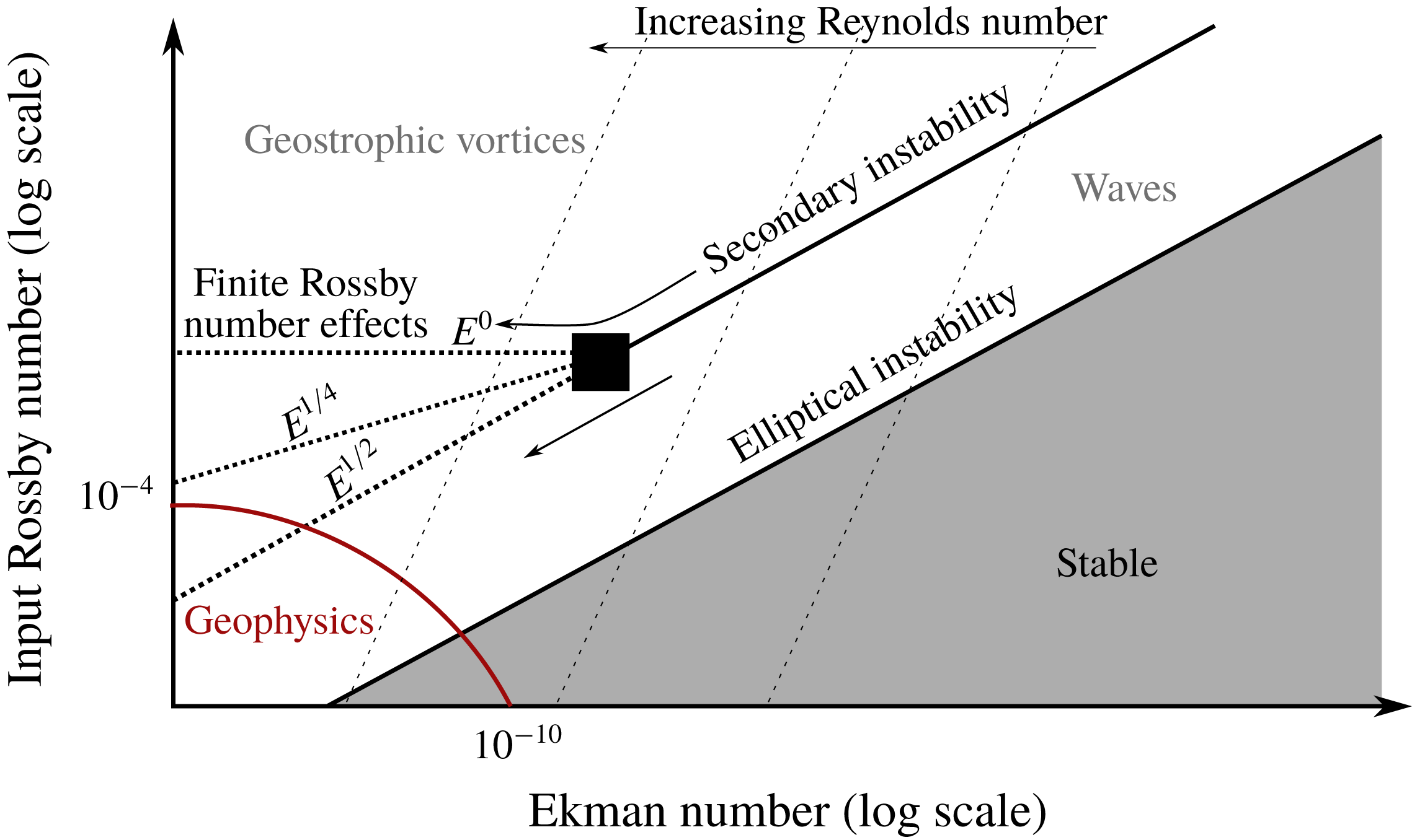
Our experimental set-up aims at understanding under which conditions these two possible nonlinear saturation states are observed. It has been designed to draw closer to low forcing and low dissipation regimes, which are relevant to planetary interiors.

3.1 The experimental set-up

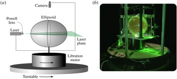
The experiments of libration-driven elliptical instability are carried out in a scaled-up version of the set-up previously implemented by Noir et al. (Reference Noir, Hemmerlin, Wicht, Baca and Aurnou2009, Reference Noir, Cébron, Bars, Sauret and Aurnou2012), Grannan et al. (Reference Grannan, Le Bars, Cébron and Aurnou2014) and Grannan et al. (Reference Grannan, Favier, Le Bars and Aurnou2017). It is depicted in figure 1. The tri-axial ellipsoid is made of two halves, each one being carved out of a polymethyl methacrylate (PMMA) block down to a sheet of thickness 7 mm with a precision of 0.05 mm, which is approximately one order of magnitude smaller than the expected boundary layer thickness. The two sides have been glued together. The lengths of the principal axes of the ellipsoid are $a=254$  mm, $b=178$  mm and $c=215$  mm, where the axis $c$ is parallel to the rotation axis. The ellipticity of the horizontal deformation $\unicode[STIX]{x1D6FD}$ is therefore 0.34. A 5 mm diameter hole in the ellipsoid allows to fill or empty it with pure water. Moreover, the ellipsoid is enclosed in a rectangular box filled with water to reduce optical distortion.

Figure 1.

Schematic cartoon (a) and photograph (b) of the experimental set-up to implement libration-driven elliptical instability. A rigid, transparent ellipsoidal container is mounted on a turntable and a secondary oscillating motor, thus producing a rotation rate with harmonic disturbances. The ellipsoid is enclosed in a rectangular box filled with water (not shown on the cartoon for clarity), which limits refraction and ensuing image distortion. For scale, the vertical extent of the ellipsoid is $2c=430$  mm. Note that there was no water in the outer box at the time the picture was taken, and that the laser sheet was vertical instead of horizontal.

In the present experiment, the ellipsoid sits on a turntable whose rotation rate ranges from 10 rotations per minute (RPM) to 40 RPM. The modulation of the rotation rate $\unicode[STIX]{x1D6FA}$ is operated by a 3.1 kW ring-style, direct-drive, servomotor (Yaskawa SGMCS-2ZN3A11). The sinusoidal motion is controlled via a card (Servopack SGD7S) and is discretised on 2000 points per period. This motor is able to produce oscillations of a system weighting around 100 kg with lateral extent of 30 cm, with a rate ranging from 0 to 180 oscillations per minute. The typical crest-to-crest amplitude of the oscillations used in this study ranges from $0^{\circ }$ to $12^{\circ }$ , although larger amplitudes can easily be reached (the system has been tested up to $50^{\circ }$ at 0.5 Hz). Relative variations of the rotation rate of the primary turntable due to the oscillations of the servo-motor do not exceed 0.4 %. The range of turntable rotation rates and libration amplitudes are indicated in table 1.

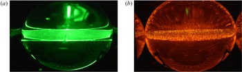
To measure the velocity of the flow, we use particle image velocimetry (PIV). A green laser beam is transformed into a 2 mm-thick homogeneous sheet with a Powell lens; the sheet cuts the ellipsoid through the equatorial plane (see figure 1) and lights PIV particles with a fluorescent coating (Cospheric UVPMS-BO-1.00, 53– $63~\unicode[STIX]{x03BC}\text{m}$ ). The fluorescent coating is such that it absorbs the green light to emit in orange; filtering out the green light allows us to capture only the particles and to get rid of parasitic reflections of the sheet on the ellipsoid (see figure 2).

High-resolution images ( $2560\times 1600$ pixels) of the laser plane are taken with a camera (Dantec SpeedSense 341) placed above the ellipsoid, the CCD sensor being at a distance of 38.7 cm from the equatorial plane. It is mounted with a 28 mm Zeiss lens. The camera is attached to a structure bound to the secondary motor, so that a fixed-shape ellipsoid is seen through the camera. The framerate used in our experiments ranges from 20 frames per second (fps) for the lowest rotation rate, to 50 fps for the highest. Image acquisition is controlled by Dantec’s software DynamicStudio. Note that the duration of a recording is limited by the available memory in the camera (32 Gbytes). The data transfer from the camera to the computer must be completed before a new recording is started, which hence prevents long and continuous acquisitions. The DynamicStudio software is used to process the images into velocity fields, via an adaptive PIV algorithm. The PIV algorithm is performed on $78\times 50$ boxes of $64\times 64$ pixels size. Note that the number of PIV particles in the ellipsoid is such that there are always approximately 3 to 5 particles inside these boxes. Lastly, both the camera and the servomotor are controlled by a computer lying on the turntable, which is monitored remotely via WiFi.

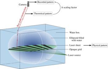
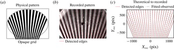
The calibration of the PIV field of view could not be achieved using a classical grid pattern, as the interior of the ellipsoid can be accessed only via a 5 mm hole. Instead, we have developed a non-invasive method based on the creation of a light pattern and on numerical ray path construction. This special method which provides a satisfying calibration is detailed in the Appendix.

A summary of the experimental parameters is given in table 1. We present in particular the values of the libration amplitude, the input Rossby number and the Ekman number which compares the effects of viscosity and Coriolis force. We emphasise the fact that our set-up allows us to reach values of the Ekman number that are approximately one order of magnitude below those of Grannan et al. (Reference Grannan, Le Bars, Cébron and Aurnou2014). This is made possible by the increase in the size of the ellipsoidal container, and the use of the most powerful servo-motor of its category.

Figure 2.

Photographs taken without (a) and with (b) an orange filter of the laser sheet lighting the fluorescent PIV particles. Using PIV particles absorbing the green light and emitting in red allows us to filter out the reflections of the sheet on the surface of the ellipsoid, thus improving the overall quality of the images taken by the high-resolution camera. Note that there was no water in the outer box at the time the pictures are taken.

Table 1.

Summary of the different input parameters used in the experiment and the corresponding dimensionless parameters. The rotation rate is in rotations per minute (RPM). The Ekman number is defined as $E=\unicode[STIX]{x1D708}/(a^{2}\unicode[STIX]{x1D6FA}_{0})$ , where $\unicode[STIX]{x1D708}$ is the viscosity of water, considered to be $1.0\times 10^{-6}~\text{m}^{2}~\text{s}^{-1}$ at room temperature; it compares the effects of viscosity to those of the Coriolis force. Note that the typical relative uncertainty on the value of the libration angle is approximately 1.5 %.

3.2 The experimental procedure

To study the nonlinear saturation of the elliptical instability, we proceed as follows. We first turn on the turntable and wait for the fluid inside the ellipsoid to reach solid-body rotation. We then turn on the secondary motor which imposes oscillations at a dimensionless rate $f=4$ with a desired amplitude $\unicode[STIX]{x0394}\unicode[STIX]{x1D711}$ . Between two experiments carried out at the same rotation rate, the secondary motor is turned off, and we wait for the remaining flow inside the ellipsoid to dissipate before starting a new run.

4.1 Measuring the libration flow

In order to characterise each experiment and to quantify the flows excited by the elliptical instability, the amplitude and the phase of the libration base flow must be precisely known. These two quantities are determined from the experimental data in the early phase of each experiment when libration is imposed but no instability has significantly grown yet: the experimental base flow is fitted to the analytical formula (2.2) in order to determine the amplitude and phase. We detail this process in the following and also illustrate the agreement between the theoretical expression and the experimental measurement of the libration base flow.

From measurements performed in the librating frame, we first define a transformed base flow $\tilde{\boldsymbol{U}}_{b}^{\ell }=(\tilde{U} ,\tilde{V})$ and a transformed position $\tilde{\boldsymbol{X}}=(\tilde{X},{\tilde{Y}})$ such that

(4.1a-d ) $$\begin{eqnarray}\tilde{U} =U/a,\quad \tilde{V}=V/b,\quad \tilde{X}=X/a,\quad {\tilde{Y}}=Y/b,\end{eqnarray}$$

where $U$ and $V$ are respectively the $X$ and $Y$ components of the measured libration base flow in the libration frame of reference. Applying this transformation to the theoretical base flow (2.2) yields

(4.2) $$\begin{eqnarray}\tilde{\boldsymbol{U}}_{b}^{\ell }=\frac{-2ab}{a^{2}+b^{2}}\unicode[STIX]{x1D6FA}_{0}\unicode[STIX]{x1D700}\sin (\unicode[STIX]{x1D6FA}_{0}ft)[-{\tilde{Y}},\tilde{X},0]=\frac{-2ab}{a^{2}+b^{2}}\unicode[STIX]{x1D6FA}_{0}\unicode[STIX]{x1D700}\sin (\unicode[STIX]{x1D6FA}_{0}ft)\tilde{r}\tilde{\boldsymbol{e}}_{\unicode[STIX]{x1D719}}=\tilde{\unicode[STIX]{x1D6FA}}(t)\tilde{r}\tilde{\boldsymbol{e}}_{\unicode[STIX]{x1D719}},\end{eqnarray}$$

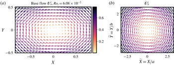
which is an oscillating solid-body rotation with effective rotation rate $\tilde{\unicode[STIX]{x1D6FA}}$ , and where we have introduced $\tilde{r}=\sqrt{\tilde{X}^{2}+{\tilde{Y}}^{2}}$ and $\tilde{\boldsymbol{e}}_{\unicode[STIX]{x1D719}}$ an orthoradial vector in the transformed coordinates. Experimental PIV fields of the base flow $\boldsymbol{U}_{b}^{\ell }$ are shown in figure 3 along with the flow transformed according to (4.1). They are in good agreement with the theoretical expressions (2.2) and (4.2).

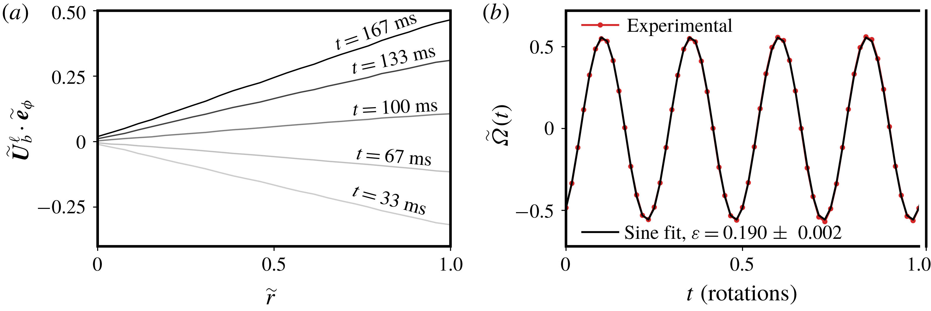
To determine the axis of rotation, the field $(\tilde{\boldsymbol{U}}_{b}^{\ell })^{2}$ is fitted to an axisymmetric parabola with adjustable central position; the location of the centre is then averaged over the whole set of velocity fields. The same transformed field is used to determine $\unicode[STIX]{x1D700}$ and the phase of the libration forcing: the position is sorted in 30 rings centred on the axis of rotation, on which the orthoradial transformed velocity is averaged. The result of this process is shown over half a libration period in figure 4(a). Fitting the averaged orthoradial velocity with a line gives the effective rotation rate $\tilde{\unicode[STIX]{x1D6FA}}(t)$ which is represented in figure 4(b). The time series of $\tilde{\unicode[STIX]{x1D6FA}}$ is fitted to a sinusoidal function to measure the amplitude of libration $\unicode[STIX]{x1D700}$ and the phase. The agreement between the experimental data and the sinusoidal function is within 1.5 % relative error.

Figure 3.

Experimental measurement of the libration base flow $\boldsymbol{U}_{b}^{\ell }$  (a) and the transformed base flow $\tilde{\boldsymbol{U}}_{b}^{\ell }$  (b) for an input Rossby number $Ro_{i}=6.08\times 10^{-2}$ . Note that $X$ and $Y$ are normalised by $a$ , and that the velocity is scaled by the typical libration velocity $Ro_{i}a\unicode[STIX]{x1D6FA}_{0}$ .

Figure 4.

(a) Experimental measurement of $\tilde{\boldsymbol{U}}_{b}^{\ell }\boldsymbol{\cdot }\tilde{\boldsymbol{e}}_{\unicode[STIX]{x1D719}}$ over half a period of libration. Each curve is labelled by the time $t$ at which the quantity is determined, given in milliseconds. (b) Experimental measurement of the effective rotation rate $\tilde{\unicode[STIX]{x1D6FA}}$ defined in (4.2) and best sinusoidal fit yielding $\unicode[STIX]{x1D700}=0.190\pm 0.002$ in this case. The fitting parameters are the phase and the amplitude of the sine. The agreement between the fit and the experimental data is within 1.5 %.

4.2 Transformation from the libration to the rotating frame

Although the camera is in the librating frame of reference for experimental convenience, the best frame to study the dynamics of the nonlinear saturation of the elliptical instability is the rotating frame in which inertial waves and the geostrophic modes are well defined. The transformation of the PIV fields from one frame to another is performed in the post-processing phase. The position in the rotating frame is deduced from the position in the libration frame by a rotation of angle $\unicode[STIX]{x1D703}_{\ell }$ as defined in (2.4). The velocity at this rotating position is computed from interpolation of the PIV field with third-order two-dimensional splines using the RectBivariateSpline function of the Python library SciPy (Jones et al. Reference Jones, Oliphant and Peterson2001). 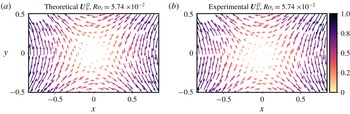This transformation also includes a velocity composition: a solid-body rotation associated with the rotation of varying angle $\unicode[STIX]{x1D703}_{\ell }$ is removed from the measured velocity. A snapshot of the base flow transformed into the rotating frame is shown in figure 5. It is compared to the theoretical base flow at the same time and the overall agreement between the two fields is satisfactory. Discrepancies may be noticed around the line $y=0$ that are due to the line where the two parts of the ellipsoid are glued together and where the optical distortion is important. Other discrepancies may be noticed in the centre where the particle displacement are small and the direction of their motion is therefore difficult to determine from the PIV algorithm. Nevertheless, the relative error between the theoretical and the experimental base flow in the rotating frame computed with $L^{2}$ norm is as low as 3 %.

Figure 5.

Snapshot of the theoretical (a) and experimental (b) libration base flow $\boldsymbol{U}_{b}^{\unicode[STIX]{x1D6FA}}$ transformed into the rotating frame, for an input Rossby number $Ro_{i}=5.74\times 10^{-2}$ . The theoretical base flow is given by formula (2.5). In this frame, the libration base flow is a standing strain field. The velocity is normalised by a typical libration velocity $Ro_{i}a\unicode[STIX]{x1D6FA}_{0}$ and the distances are normalised by $a$ .

5.1 Kinetic energy time series

To describe in general the saturation of the libration-driven elliptical instability, we track the evolution of the kinetic energy over time. In particular, we focus on the kinetic energy of the fluctuations around the libration base flow. These fluctuations are measured directly in the libration frame, i.e. there is no need to proceed to a change of frame of reference to carry out this measurement. Let us call $\boldsymbol{u}$ the fluctuations, such that the total flow $\boldsymbol{U}^{\ell }$ in the libration frame of reference is written

(5.1) $$\begin{eqnarray}\boldsymbol{U}^{\ell }(\boldsymbol{X})=\boldsymbol{U}_{b}^{\ell }(\boldsymbol{X})+\boldsymbol{u}(\boldsymbol{X}).\end{eqnarray}$$

The flow in the rotating frame is deduced from (5.1) by a coordinate rotation $\boldsymbol{X}\mapsto \boldsymbol{x}$ and a velocity composition with the solid-body rotation

(5.2) $$\begin{eqnarray}\boldsymbol{U}_{rot}=\unicode[STIX]{x1D6FA}_{0}\unicode[STIX]{x1D700}\sin (\unicode[STIX]{x1D6FA}_{0}ft)[-y,x,0].\end{eqnarray}$$

The total flow in the rotating frame of reference, $\boldsymbol{U}^{\unicode[STIX]{x1D6FA}}$ , is therefore

(5.3) $$\begin{eqnarray}\boldsymbol{U}^{\unicode[STIX]{x1D6FA}}(\boldsymbol{x})=\boldsymbol{U}_{b}^{\ell }(\boldsymbol{x})-\boldsymbol{U}_{rot}(\boldsymbol{x})+\boldsymbol{u}(\boldsymbol{x})=\boldsymbol{U}_{b}^{\unicode[STIX]{x1D6FA}}(\boldsymbol{x})+\boldsymbol{u}(\boldsymbol{x}),\end{eqnarray}$$

where $\boldsymbol{U}_{b}^{\unicode[STIX]{x1D6FA}}(\boldsymbol{x})$ is the base flow measured in the mean rotation rate frame of reference. It is therefore equivalent to measure the kinetic energy of the fluctuations in these two frames. We therefore define a fluctuation kinetic energy ${\mathcal{E}}$ and a base flow kinetic energy ${\mathcal{E}}_{b}$ ,

(5.4a,b ) $$\begin{eqnarray}{\mathcal{E}}=\frac{1}{2}\langle \boldsymbol{u}^{2}\rangle \quad \text{and}\quad {\mathcal{E}}_{b}=\frac{f\unicode[STIX]{x1D6FA}_{0}}{2\unicode[STIX]{x03C0}}\int _{0}^{2\unicode[STIX]{x03C0}/f\unicode[STIX]{x1D6FA}_{0}}\left\langle \frac{1}{2}(\boldsymbol{U}_{b}^{\unicode[STIX]{x1D6FA}})^{2}\right\rangle \,\text{d}t,\end{eqnarray}$$

where the operation $\langle \cdot \rangle$ denotes a summation over all the points of the velocity field obtained from the PIV measurements, located in the equatorial plane of the ellipsoid.

Figure 6.

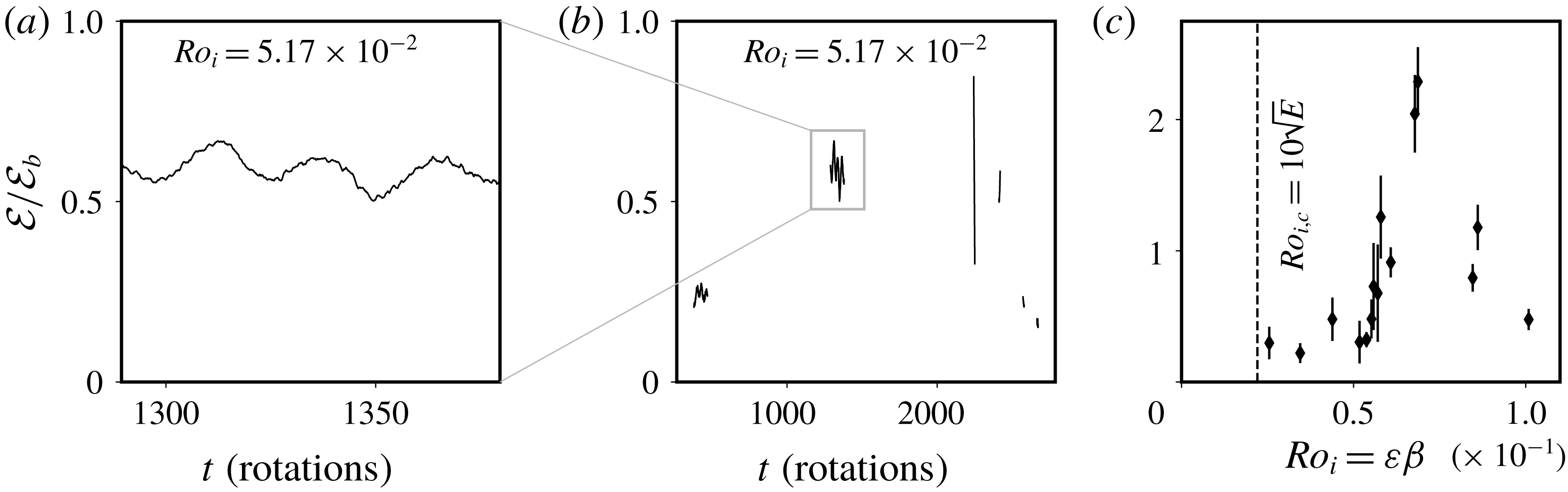
(a) Kinetic energy variation over a hundred rotation times at an Ekman number $E=5.0\times 10^{-6}$ , $f=4$ and $Ro_{i}=5.17\pm 0.07\times 10^{-2}$ . (b) Several successive time series of the kinetic energy for the same experimental run as in (a). This panel highlights the long-time variability of the saturation flow. The minimum separation between two successive recordings of the velocity field is set by the time needed to transfer the data from the camera to the computer. This data set comprises long (5476 images) and short (500 images) recordings at a frame rate of 30 fps. Note that these time series include the one shown in (a). For both panels, the time series are low-pass filtered by a sliding average over one rotation period. (c) Mean value of the kinetic energy in the saturation phase of the instability at 30 RPM and $f=4$ for all the experimental values of the input Rossby number $Ro_{i}$ . The error bar is given by the standard deviation of kinetic energy considering all successive recordings for each experiment (see for instance the central panel). The vertical dashed line gives the approximate viscous threshold of the instability according to Le Bars et al. (Reference Le Bars, Lacaze, Le Dizès, Le Gal and Rieutord2010) and Favier et al. (Reference Favier, Grannan, Le Bars and Aurnou2015), which is $Ro_{i,c}\sim 10\sqrt{E}$ , and below which the flow is experimentally observed to be stable.

The result of computing the ratio ${\mathcal{E}}/{\mathcal{E}}_{b}$ is shown in figure 6 where we represent time series of this quantity and its mean value for several experiments at an Ekman number $E=5.0\times 10^{-6}$ (see table 1). The quantity ${\mathcal{E}}$ undergoes fluctuations over time, be it at time scales as short as the rotation period or at very long times scales, similar to the slow nonlinear time scale $2\unicode[STIX]{x03C0}(Ro_{i}\unicode[STIX]{x1D6FA})^{-1}$ ranging from 60 to 200 rotation periods. In addition, the ratio ${\mathcal{E}}/{\mathcal{E}}_{b}$ is of order 1, which indicates that the amplitude of the fluctuations is of order $Ro_{i}$ . This result is expected from balancing the nonlinear term $|\boldsymbol{u}\boldsymbol{\cdot }\unicode[STIX]{x1D735}\boldsymbol{u}|\sim u^{2}/\unicode[STIX]{x1D706}$ (where $\unicode[STIX]{x1D706}$ is the resonant mode wavelength) with forcing terms $|\boldsymbol{U}_{b}^{\unicode[STIX]{x1D6FA}}\boldsymbol{\cdot }\unicode[STIX]{x1D735}\boldsymbol{u}+\boldsymbol{u}\boldsymbol{\cdot }\unicode[STIX]{x1D735}\boldsymbol{U}_{b}^{\unicode[STIX]{x1D6FA}}|\sim Ro_{i}u/\unicode[STIX]{x1D706}$ leading to a saturation velocity perturbation $u\sim Ro_{i}$ . A similar saturation amplitude was already observed in previous experiments and simulations (Barker & Lithwick Reference Barker and Lithwick2013; Grannan et al. Reference Grannan, Favier, Le Bars and Aurnou2017). These two features of the kinetic energy attest to the fact that the saturation phase is dominated by nonlinear transfers, and is potentially turbulent. Variations around the simple scaling ${\mathcal{E}}/{\mathcal{E}}_{b}=O(1)$ are noticeable in figure 6 but remain difficult to explain since our set-up only allows us to measure horizontal motions in a plane. In particular, the vertical motions along the rotation axis and their dependence on $Ro_{i}$ are not accessible.

In this section, we are interested in the saturation flow for forcing amplitudes that are above the threshold of the instability but which remain relatively small (typically $Ro_{i}<5.58\times 10^{-2}$ at $E=5.0\times 10^{-6}$ ). Figure 6(c) proves that even close to the threshold the kinetic energy of the perturbation flow $\boldsymbol{u}$ reaches significant values ( ${\mathcal{E}}/{\mathcal{E}}_{b}>0.3$ ) and undergoes temporal variability.

5.2 Spectral content of the flow: inertial waves in resonant interaction

To refine the analysis of the nonlinear saturation flow we explore its spectral content in the temporal domain and in the rotating frame of reference. It is a natural analysis to perform because many features of the flow have a specific frequency signature: the libration forcing appears at $\unicode[STIX]{x1D714}=f=4$ , and inertial waves are restrained to the domain $[-2,2]$ (time being normalised by the rotation time scale $\unicode[STIX]{x1D6FA}_{0}^{-1}$ ).

To determine the spectral content of the flow, we randomly select a set of 300 locations in the rotating frame of reference where the two components of the velocity are recorded. Prior to performing the temporal Fourier transform, the local velocity time series are multiplied by the Hann windowing function ${\mathcal{H}}$ defined as

(5.5) $$\begin{eqnarray}{\mathcal{H}}(t)=\frac{1}{2}-\frac{1}{2}\cos \left(\frac{2\unicode[STIX]{x03C0}}{T}t\right),\end{eqnarray}$$

where we have assumed that the local velocity time series span a time interval $[0,T]$ . This windowing avoids the emergence of artificial secondary maxima around peaked frequencies, due to the non-periodicity of the experimental signals. Lastly, we perform an ensemble average over the set of 300 power spectra, yielding a quantity denoted as $\hat{E}(\unicode[STIX]{x1D714})$ . These power spectra are scaled by a typical local energy of the base flow $e_{b}$ that is defined as the total base flow kinetic energy ${\mathcal{E}}_{b}$ divided by the number of PIV boxes composing the field of view.

Figure 7.

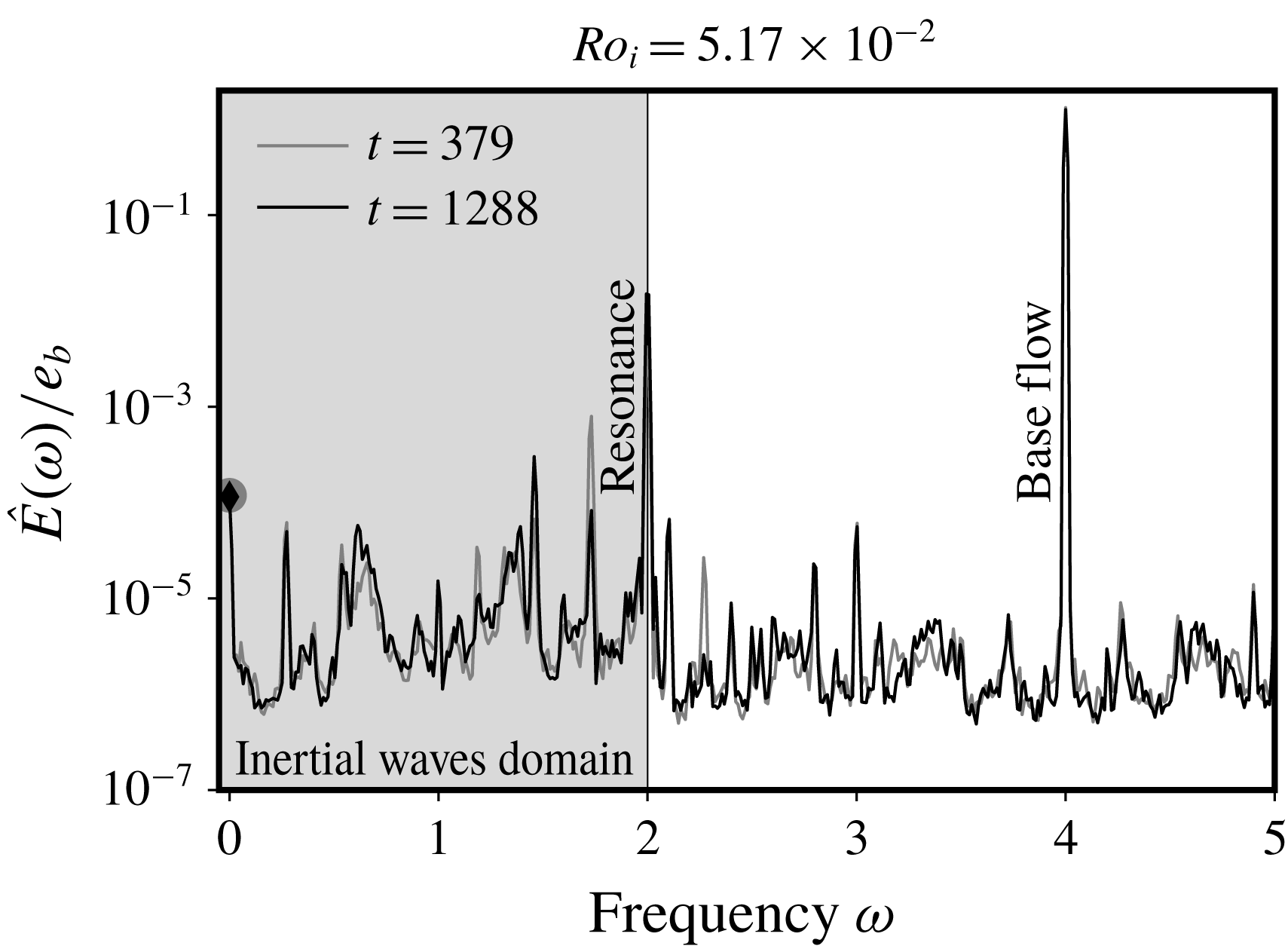
Ensemble average of temporal spectra at a forcing amplitude $Ro_{i}=5.17\times 10^{-2}$ , a libration frequency $f=4$ and an Ekman number $E=5.0\times 10^{-6}$ . The frequency $\unicode[STIX]{x1D714}$ is given in rotation units, so that $\unicode[STIX]{x1D714}=1$ corresponds to a frequency of $\unicode[STIX]{x1D6FA}_{0}$ . Two different power spectra are displayed, they correspond to two different recordings around a time $t$ indicated in rotation periods in order to enhance robust features. Among the clear peaks are the base flow at $\unicode[STIX]{x1D714}=f=4$ peaking at $\hat{E}(f)/e_{b}\sim 1$ , and the resonant mode at $\unicode[STIX]{x1D714}=f/2=2$ . The shaded area denotes the domain of existence of inertial waves. The two symbols at $\unicode[STIX]{x1D714}=0$ highlight the value taken by both spectra at this frequency, their colour being the same as the corresponding spectra. The typical frequency resolution is approximately $1.1\times 10^{-2}$ .

A typical result of this process for an Ekman number $E=5.0\times 10^{-6}$ , a libration frequency $f=4$ and an input Rossby number $Ro_{i}=5.17\times 10^{-2}$ is shown in figure 7. As anticipated, the peaks associated with the libration flow ( $\unicode[STIX]{x1D714}=f=4$ ) and the resonant modes ( $\unicode[STIX]{x1D714}=f/2=2$ ) appear clearly in the power spectra. In addition, superposing power spectra for the same experiment but at different times reveals the overall reproducibility of this measurement.

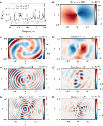
The peaks, in particular in the inertial modes range, and the low background noise, indicate that the saturation at low forcing is chaotic or weakly turbulent, and includes persistent inertial modes. Furthermore, we notice in figure 8(a) that their position is not random but persists at different Ekman numbers provided the forcing remains small. Besides, the peaks can be paired together so that their frequencies $\unicode[STIX]{x1D714}_{1}$ and $\unicode[STIX]{x1D714}_{2}$ satisfy

(5.6) $$\begin{eqnarray}\unicode[STIX]{x1D714}_{1}+\unicode[STIX]{x1D714}_{2}=2.\end{eqnarray}$$

This suggests that the paired structures are inertial waves in triadic resonant interactions with the resonant mode, as explained in § 2.3 (see in particular relation (2.12)).

Figure 8.

(a) Power spectra with labelled peaks. The spectrum at $E=5.0\times 10^{-6}$ is the same as in figure 7 ( $Ro_{i}=5.17\times 10^{-2}$ ). The $E=7.4\times 10^{-6}$ spectrum is determined from an experiment at input Rossby number $Ro_{i}=5.90\times 10^{-2}$ , it has been vertically shifted to facilitate the comparison. Several pairs of triadic resonance relations can be noticed, such as $0.27+1.73$ , $0.54+1.46$ , $0.61+1.39$ and $0.66+1.34$ . (b) Azimuthal component of the resonant wave. (c–g) Pairs of structures $\hat{\boldsymbol{u}}(\boldsymbol{r};\unicode[STIX]{x1D714})$ satisfying the triadic resonance condition on the frequency (relation (2.12)). For each frequency, including $\unicode[STIX]{x1D714}=2$ , we show the component which has the largest amplitude among the imaginary and real parts of the radial ( $\hat{u} _{r}$ ) and azimuthal ( $\hat{u} _{\unicode[STIX]{x1D719}}$ ) velocities. Lastly, in all velocity maps, distance is normalised by $a$ and velocity by $Ro_{i}a\unicode[STIX]{x1D6FA}_{0}$ .

To further support our claim that the temporal power spectra present evidence for triadic resonant interactions, we extract from the PIV fields the structure at the peaked frequency. The structure oscillating at frequency $\unicode[STIX]{x1D714}$ , i.e. the Fourier component of the flow at this frequency $\hat{\boldsymbol{u}}(\unicode[STIX]{x1D714})$ , is extracted using the following operation:

(5.7) $$\begin{eqnarray}\hat{\boldsymbol{u}}(\boldsymbol{r};\unicode[STIX]{x1D714})=\int _{t_{0}}^{t_{1}}\boldsymbol{U}^{\unicode[STIX]{x1D6FA}}(\boldsymbol{r},t)\text{e}^{\text{i}\unicode[STIX]{x1D714}t}\,\text{d}t,\end{eqnarray}$$

where $t_{0}$ and $t_{1}$ are the start and end times of a PIV recording and $\boldsymbol{U}$ is the total velocity field measured in the rotating frame. The result of such a process is shown for several pairs of frequencies in figure 8. The spatial structures extracted at the peaked frequencies show a spatially periodic organisation which is typical of inertial modes. Comparison with theoretical structures remains nevertheless complicated because the viscous inertial modes of a tri-axial ellipsoid are not known theoretically and require complicated numerical computation (Vidal & Cébron Reference Vidal and Cébron2017; Vidal et al. Reference Vidal, Cébron and Schaeffer2017).

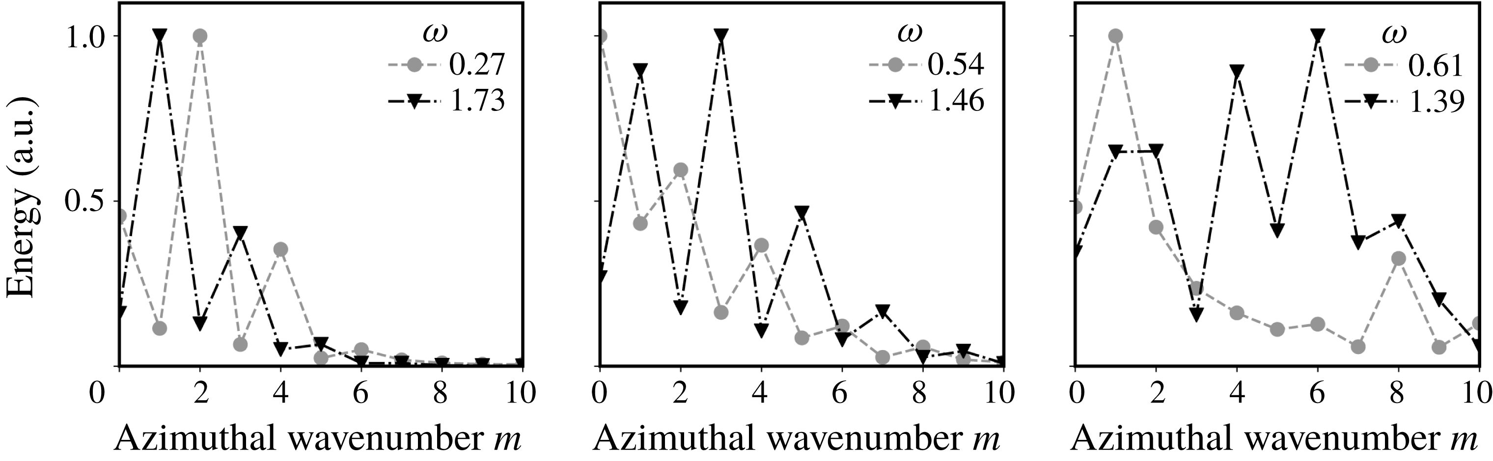
In addition, the ability of the paired modes to interact with the resonant one may be assessed by examining their principal azimuthal wavenumbers. The latter is determined for a mode $\hat{\boldsymbol{u}}(\boldsymbol{r};\unicode[STIX]{x1D714})$ by transformation into polar coordinates $(r,\unicode[STIX]{x1D719})$ , and Fourier transform along $\unicode[STIX]{x1D719}$ to obtain the following decomposition of the mode:

(5.8) $$\begin{eqnarray}\hat{\boldsymbol{u}}(r,\unicode[STIX]{x1D719};\unicode[STIX]{x1D714})=\mathop{\sum }_{m}\hat{\boldsymbol{u}}_{m}(r)\text{e}^{\text{i}m\unicode[STIX]{x1D719}}.\end{eqnarray}$$

Because the fluid container is not invariant under rotation, such decomposition necessarily comprises more than one wavenumber, but we can still identify the largest contributions to the azimuthal wavenumber decomposition by computing the energy of the coefficients by radial integration, that is,

(5.9) $$\begin{eqnarray}\int _{r<r_{max}}|\hat{\boldsymbol{u}}_{m}(r)|^{2}r\,\text{d}r,\end{eqnarray}$$

where $r_{max}$ is a maximum radius over which the integration is performed. We choose $r_{max}=0.5a$ , which approximately corresponds to the radius of the largest circle fitting inside the PIV field.

Note that no coordinate transformation correcting for the elliptical distortion is applied. Such a transformation is not required as it complicates the wavenumber decomposition of smaller scales modes such as the one at $\unicode[STIX]{x1D714}=0.61$ (see figure 8 g), and leads to qualitatively similar decomposition for larger scales modes such as those shown in figure 8(c–f).

Calling $m_{i}$ the wavenumber of the resonant mode (here $\pm 1$ , see figure 8 b) and $m_{j,k}$ the daughter waves’, significant nonlinear interaction is ensured provided that

(5.10) $$\begin{eqnarray}m_{j}+m_{k}=m_{i},\end{eqnarray}$$

which is very similar to the condition on frequency (2.12). In the present case, the mode $i$ is the resonant one, for which $m_{i}=\pm 1$ , so that the difference between absolute value of the main wavenumbers of paired modes should be $\pm 1$ . The result of computing the azimuthal wavenumber decomposition is shown in figure 9, and is, at least for two pairs of modes, consistent with the relation (5.10).

Figure 9.

Computation of the azimuthal wavenumber decomposition (see formulae (5.8) and (5.9)) of the paired structures shown in figure 8. The energy contained in the wavenumbers is shown in arbitrary units. Note that these maps are symmetric respective to $m=0$ , so that the energy contained in the $m$ and $-m$ modes is the same. For these structures to significantly interact with the resonant mode, the gap between the displayed principal wavenumbers numbers must be $\pm 1$ (see relation (5.10)), which is indeed observed for the first two pairs, but less obvious for the last one. Note that in the computation of the energy, the radial integration has been restricted to radii below $0.5a$ , which corresponds to the radius of the largest circle fitting inside the PIV fields.

Lastly, regardless of considerations on the azimuthal structures, it is striking in figure 8 that only modes with similar scales are observed to couple in triadic resonances. This is coherent with the fact that, as the resonant mode at $\unicode[STIX]{x1D714}=2$ has almost no horizontal variations, the two daughter modes must have matching horizontal wavenumbers to ensure a significant spatial overlap and efficient energy transfer.

To conclude, the spatio-temporal analysis of the flow at low forcing amplitudes provides significant evidence that, in this regime, the nonlinear saturation of the elliptical instability is a superposition of daughter waves that are in triadic resonant interaction with the unstable mode. This state is robust as the Ekman number is changed, provided the forcing remains small. It could be seen as discrete inertial wave turbulence (Kartashova Reference Kartashova2009), which should lead to inertial wave turbulence in the low dissipation and forcing regime, as shown by Le Reun et al. (Reference Le Reun, Favier, Barker and Le Bars2017) with an idealised numerical model.

To finish with, one could argue that in the present set-up, some hypotheses of classical wave turbulence theory (Nazarenko Reference Nazarenko2011) are not satisfied. First, the flow is not statistically homogeneous in space, as we observe modes whose structures are influenced by boundaries. It is neither statistically homogeneous in time because the system is by essence forced at a single frequency. Lastly, as discussed above, dissipation is still too high and prevents energy cascade in a large range of scales. Some of these limitations are inherent to the experimental approach used here, but may be irrelevant in the asymptotic geophysical regime. Note also that none of the previous numerical or experimental set-ups studying rotating turbulence have yet reported a regime dominated by inertial waves only and without a dominant geostrophic component (see Godeferd & Moisy (Reference Godeferd and Moisy2015) for a review) as we observe here. We thus argue that this work is a first step towards reaching an inertial wave turbulence regime.

6.1 Spectral content of the saturation flow at large forcing amplitude

Figure 10.

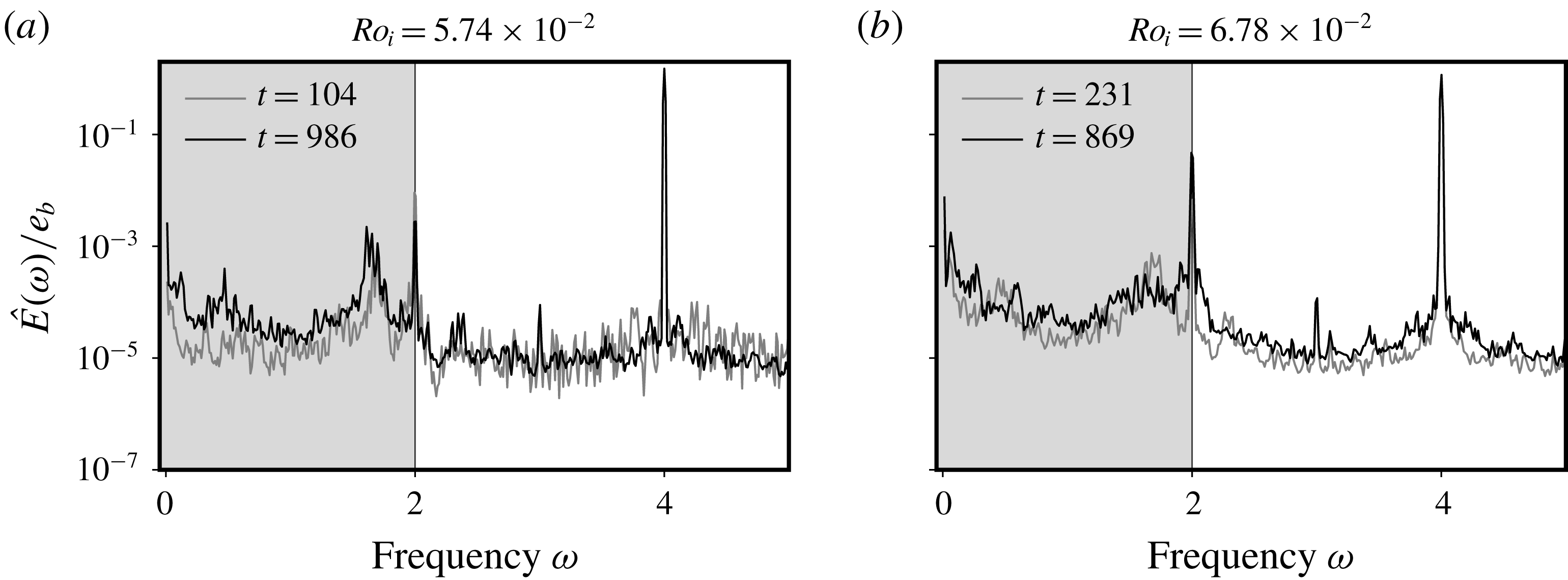
Temporal spectra of the saturation flow obtained at $E=5.0\times 10^{-6}$ with the same process as in figure 7, but with higher forcing amplitudes or $Ro_{i}$ values. As earlier, the inertial wave domain is highlighted in grey, and the base flow and resonant peaks are clearly identifiable.

We reproduce the temporal analysis of the saturation flow detailed in § 5.2, now applied to the larger forcing experiments. Several striking changes appear in these power spectra displayed in figure 10 compared to what has been obtained at lower forcing (see figure 7). First, the number of peaks in the inertial wave domain is reduced, and the remaining ones are wider. Moreover, the ratio between the background level and the forcing peak (at $\unicode[STIX]{x1D714}=f=4$ ) increases with the forcing, thus suggesting that the flow becomes more turbulent. Lastly, the gap between the mean flow (at $\unicode[STIX]{x1D714}=0$ ) and the resonant mode reduces from two to less than one order of magnitude between low (figure 7) and large forcing.

It is thus clear that the saturation flow has transitioned towards another regime: the many triadic resonances that clearly appeared in the inertial modes domain in figures 7 and 8 are no longer present.

6.2 The emergence of a strong geostrophic anticyclonic vortex

Figure 11.

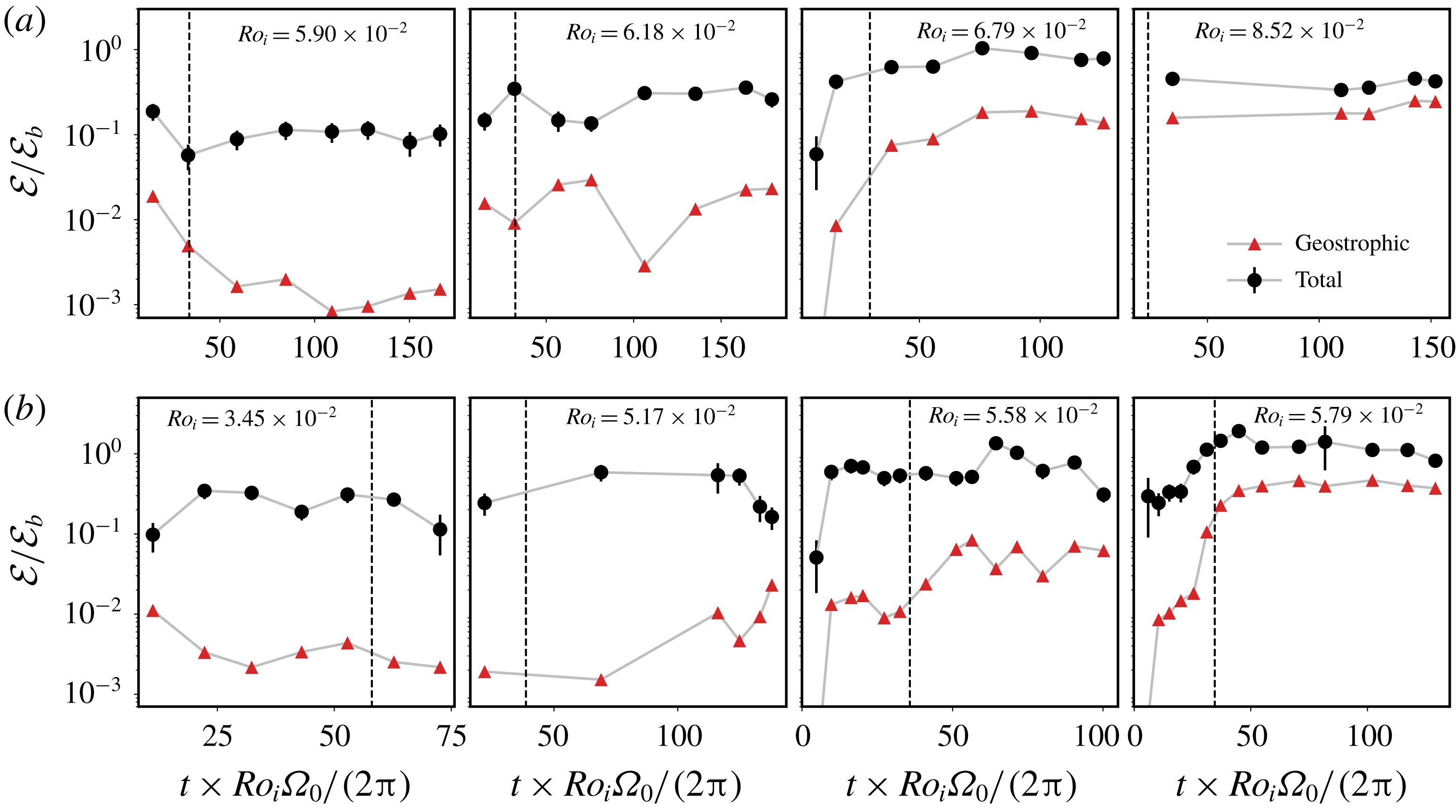
Long-term evolution of the kinetic energy of the total perturbation flow $\boldsymbol{u}$ (see § 5.1) and the geostrophic component for experiments carried out at $E=7.4\times 10^{-6}$ (a) and $E=5.0\times 10^{-6}$ (b). Each experimental run consists in a succession of recordings from which the average total kinetic energy and the mean flow kinetic energy are extracted. They are normalised by the base flow energy ${\mathcal{E}}_{b}$ defined in (5.3). Note that the spectra shown in figures 7 and 8(a) correspond to the time series $E=5.0\times 10^{-6}$ , $Ro_{i}=5.17\times 10^{-2}$ and $E=7.4\times 10^{-6}$ , $Ro_{i}=5.90\times 10^{-2}$ . The error bars on the total kinetic energy correspond to its standard deviation over each recording. For each experiment, time is normalised by a nonlinear time scale $2\unicode[STIX]{x03C0}/(\unicode[STIX]{x1D6FA}_{0}Ro_{i})$ . The vertical dashed line denotes a long nonlinear time scale $2\unicode[STIX]{x03C0}/(\unicode[STIX]{x1D6FA}_{0}Ro_{i}^{2})$ .

The key to the transition out of the wave-dominated regime is the rise of the geostrophic mean flow amplitude, a feature noticed in figure 10. The aim of the present paragraph is to explain the properties of this particular component of the saturation flow and to quantify its evolution when the forcing amplitude, or equivalently $Ro_{i}$ , is changed.

The geostrophic component of the flow $\overline{\boldsymbol{U}}$ is extracted by time averaging the velocity fields over a sufficiently long time period. It is found that 5 rotation periods are sufficient to average a representative mean flow, although we perform the averaging operation over the full length of a recording, which typically ranges from tens to approximately a hundred rotation periods.

As an experimental run comprises several successive recordings, we can characterise the long-term evolution of the geostrophic component of the flow. We show in figure 11 time series of the kinetic energy of the geostrophic component extracted from the saturation flow for increasing forcing amplitude or $Ro_{i}$ . The average over each recording of kinetic energy of the total perturbation flow $\boldsymbol{u}$ , computed in § 5.1, is also given for reference. To facilitate the comparison between experiments with different forcing amplitudes $Ro_{i}$ , time is normalised by the nonlinear time scale $2\unicode[STIX]{x03C0}/(\unicode[STIX]{x1D6FA}_{0}Ro_{i})$ . For the majority of the experiments, both the total and mean flow kinetic energy time series reach a statistically steady state within a few tens of nonlinear time scales. Furthermore, we notice a gradual and clear change in the energy of the mean flow as $Ro_{i}$ is increased. At low forcing amplitude, the geostrophic kinetic energy remains approximately two orders of magnitude smaller than the base flow kinetic energy. A quite rapid transition is observed between $Ro_{i}=5.90\times 10^{-2}$ and $Ro_{i}=6.79\times 10^{-2}$ at $E=7.4\times 10^{-6}$ , and between $Ro_{i}=5.17\times 10^{-2}$ and $Ro_{i}=5.79\times 10^{-2}$ at $E=5.0\times 10^{-6}$ , where the geostrophic kinetic energy increases by two orders of magnitude.

Figure 12.

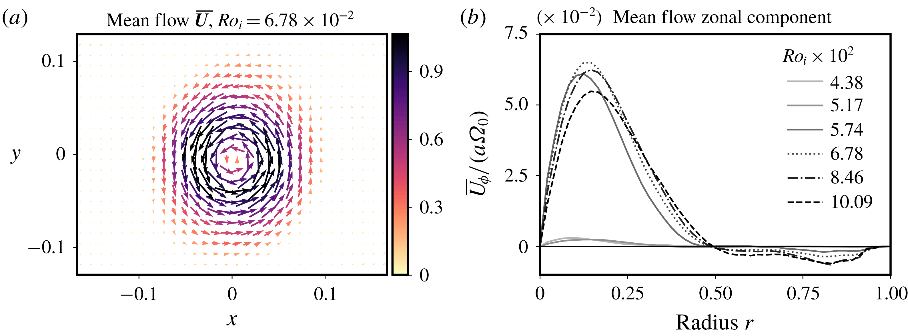
(a) Mean flow $\overline{\boldsymbol{U}}$ extracted by averaging of the saturation flow observed at an Ekman number $E=5.0\times 10^{-6}$ and an input Rossby number $Ro_{i}=6.78\times 10^{-2}$ . The colour scale of the arrows gives the norm of the velocity, normalised by the base flow velocity $Ro_{i}\unicode[STIX]{x1D6FA}a$ . The rotation of the turntable being clockwise, the observed vortex is an anticyclone. Lengths are normalised by $a$ . (b) Zonal average of the mean flow orthoradial velocity at the same Ekman number; it is normalised by $a\unicode[STIX]{x1D6FA}_{0}$ , independently of $Ro_{i}$ , which enhances the sharp change in the mean flow amplitude.

Regardless of the forcing amplitude and the rotation rate, the mean flow $\overline{\boldsymbol{U}}$ always adopts the shape of an anticyclonic zonal wind, i.e. a stationary flow with mostly azimuthal velocity and which rotates counter-clockwise (while the rotation of the turntable is clockwise). A typical view of the mean flow is given in figure 12(a) for a value of the forcing amplitude $Ro_{i}$ where the geostrophic energy reaches a high value. To better quantify the structure and the amplitude of the mean flow $\overline{\boldsymbol{U}}$ , we consider its zonal average $\overline{U}_{\unicode[STIX]{x1D719}}(r)$ , defined as

(6.1) $$\begin{eqnarray}\overline{U}_{\unicode[STIX]{x1D719}}(r)=\frac{1}{2\unicode[STIX]{x03C0}}\int _{\unicode[STIX]{x1D719}=0}^{2\unicode[STIX]{x03C0}}\overline{\boldsymbol{U}}\boldsymbol{\cdot }\boldsymbol{e}_{\unicode[STIX]{x1D719}}\,\text{d}\unicode[STIX]{x1D719}.\end{eqnarray}$$

It is computed by dividing the PIV field in concentric rings of radius $r$ and averaging the quantity $\overline{\boldsymbol{U}}\cdot \boldsymbol{e}_{\unicode[STIX]{x1D719}}$ on each ring. This zonal average is pictured in figure 12(b). We retrieve a clear transition from the lowest values of the input Rossby number ( $Ro_{i}<5.28\times 10^{-3}$ in figure 12 b) with very weak vortex amplitude to larger values where a strong mean flow develops. A similar strong anticyclonic vortex was also observed by Grannan et al. (Reference Grannan, Le Bars, Cébron and Aurnou2014) and Favier et al. (Reference Favier, Grannan, Le Bars and Aurnou2015) in the turbulent saturation of the libration-driven elliptical instability, at Ekman numbers ranging from $5\times 10^{-5}$ to $10^{-4}$ and at a single input Rossby number $Ro_{i}=0.272$ .

To further quantify the transition, we introduce two diagnostic quantities. The first one is the root mean square value of the mean flow ${\mathcal{U}}_{rms}^{2d}$ defined as

(6.2) $$\begin{eqnarray}({\mathcal{U}}_{rms}^{2d})^{2}=\langle \overline{\boldsymbol{U}}^{2}\rangle ,\end{eqnarray}$$

where the symbol $\langle \,\cdot \,\rangle$ denotes averaging over the whole PIV field, which we recall is in the equatorial plane of the ellipsoid. The second one is the central vorticity of the mean flow to quantify the central rotation rate of the geostrophic vortex. The average radial vorticity profile $\overline{\unicode[STIX]{x1D714}}_{z}(r)$ is computed as

(6.3) $$\begin{eqnarray}\overline{\unicode[STIX]{x1D714}}_{z}(r)=\frac{\overline{U}_{\unicode[STIX]{x1D719}}}{r}+\frac{\text{d}\overline{U}_{\unicode[STIX]{x1D719}}}{\text{d}r}.\end{eqnarray}$$

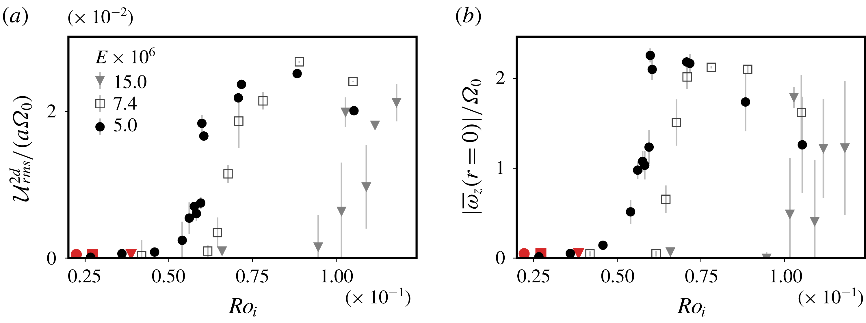
Close to the centre, it is computed via fitting a third-order polynomial to the zonal velocity profile $\overline{U}_{\unicode[STIX]{x1D719}}$ , as with those depicted in figure 12; $\overline{\unicode[STIX]{x1D714}}_{z}(r=0)$ is then twice the first-order coefficient of the polynomial fit. For each experiment, these two diagnostic quantities are averaged over the last half of the recordings, for which a statistically steady state is usually obtained (see figure 11). The evolution of the mean flow r.m.s. and central vorticity is shown in figure 13. In (a,b), a clear transition from a negligible amplitude mean flow to a strong mean flow is observed, with a critical Rossby number $Ro_{i,c}$ depending on the Ekman number. This proves the existence of a secondary transition of the geostrophic anticyclone that builds on the turbulent saturation of the libration-driven elliptical instability.

Figure 13.

(a) Experimental measurements of the root mean square (r.m.s.) value ${\mathcal{U}}_{rms}^{2d}$ of the mean flow, defined in (6.2), as a function of the input Rossby number $Ro_{i}$ ; it is normalised by $a\unicode[STIX]{x1D6FA}_{0}$ instead of $Ro_{i}a\unicode[STIX]{x1D6FA}_{0}$ so that the amplitude of the r.m.s. value is independent of $Ro_{i}$ . The red symbols show the approximate critical Rossby number $10\sqrt{E}$ at the Ekman number corresponding to the shape of the symbol. (b) Experimental measurements of the central vorticity of the mean flow $\overline{\unicode[STIX]{x1D714}}_{z}(r=0)$ (see formula (6.3)) as a function of $Ro_{i}$ . It is normalised by the rotation rate $\unicode[STIX]{x1D6FA}_{0}$ . Note the mean flow is an anticyclonic vortex and has therefore a vertical vorticity opposite to the rotation. For both panels, the error bars indicate the typical variability in the saturation phase by computing the standard deviation of ${\mathcal{U}}_{rms}^{2d}$ and $\overline{\unicode[STIX]{x1D714}}_{z}(r=0)$ when more than one data set was available.

Below the secondary transition, the variations of the central vorticity with $Ro_{i}$ do not match any scaling $\overline{\unicode[STIX]{x1D714}}_{z}(r)\propto Ro_{i}^{2}$ that has been proposed and measured for mean flows driven by the libration base flow alone (Busse Reference Busse2010; Sauret et al. Reference Sauret, CéBron, Morize and Le Bars2010; Sauret & Le Dizès Reference Sauret and Le Dizès2013) or by nonlinear self-interaction of a single inertial mode in the laminar regime (Tilgner Reference Tilgner2007; Morize et al. Reference Morize, Le Bars, Le Gal and Tilgner2010; Sauret et al. Reference Sauret, Le Bars and Le Gal2014). This shows that the mean flow does not result from nonlinear self-interaction in the boundary layer of simple structures such as the base flow or a single inertial mode.

For input Rossby numbers above the secondary transition, the central vorticity reaches a plateau at the value of ${\sim}-2\unicode[STIX]{x1D6FA}_{0}$ , meaning that the core of the vortex cancels out on average the rotation of the fluid. It is striking that the central vorticity saturates at this value for which anticyclones are marginally stable according to the Rayleigh criterion for centrifugal instability (Afanasyev & Peltier Reference Afanasyev and Peltier1998; Drazin & Reid Reference Drazin and Reid2004). Such a saturation value emerging out of a turbulent saturation may be reminiscent of self-organised criticality (Bak, Tang & Wiesenfeld Reference Bak, Tang and Wiesenfeld1987), an idea that is for instance invoked in stratified turbulence where flows are thought to be maintained close to marginal stability respective to shear instability (see for instance Salehipour, Peltier & Caulfield (Reference Salehipour, Peltier and Caulfield2018)).

Beyond this plateau, a slight decrease of both the r.m.s. and the central vorticity of the mean flow is observed at higher $Ro_{i}$ , at least for Ekman numbers $E=5.0\times 10^{-6}$ and $E=7.4\times 10^{-6}$ . It is possibly linked to a transition from rotating to isotropic turbulence as the Rossby number draws closer to 1 (Yokoyama & Takaoka Reference Yokoyama and Takaoka2017). As observed for instance by Barker & Lithwick (Reference Barker and Lithwick2013), increasing the amplitude of the forcing leads to the destabilisation of the strong vortices produced by the saturation of the elliptical instability. Nevertheless, in our set-up, the transition from a purely two-dimensional vortex to three-dimensional structures with possible vertical motion is difficult to further quantify.

6.3 Building a regime diagram of the saturation flow

Figure 14.

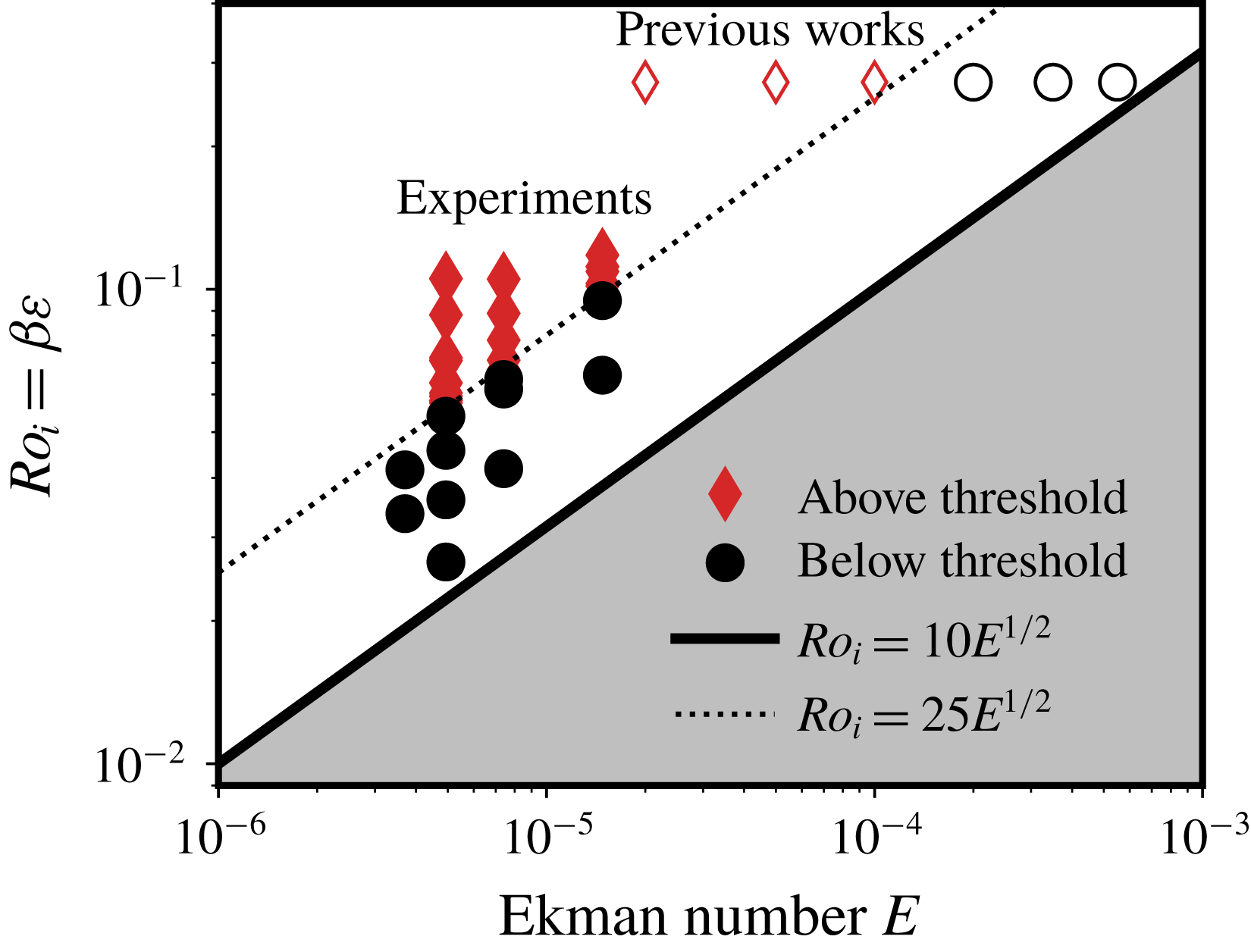
Experimental determination of the position of the secondary transition of the geostrophic vortex as a function of the Ekman number $E$ and the input Rossby number $Ro_{i}$ . The shaded area denotes the values of the control parameters for which the libration base flow is stable, its upper bound is a line $Ro_{i}=10\sqrt{E}$ . The empty symbols stand for the control parameters of Grannan et al. (Reference Grannan, Le Bars, Cébron and Aurnou2014) and Favier et al. (Reference Favier, Grannan, Le Bars and Aurnou2015) for which a central anticyclone similar to what is observed here is obtained in the nonlinear saturation. As it can be noticed in the data of Favier et al. (Reference Favier, Grannan, Le Bars and Aurnou2015) (figure 5), there exists a sharp increase in the central vorticity; points below this transition are black circles and points above are red diamonds. To determine the location of the transition in our experiments, we consider that the threshold is reached when the energy of the mean flow is larger than 15 % of its largest value over a whole set of experiments carried out at the same Ekman number but different input Rossby numbers. Varying this threshold, say from 5 % to 20 %, may change the nature of the points around the dashed line, but does not affect the overall trend for the separation between the two regimes.

As noted in figure 13, the secondary transition between a wave-dominated and a geostrophic-dominated regimes is characterised by a sudden increase in the mean flow r.m.s. velocity and vorticity. The critical value of $Ro_{i}$ at which this transition occurs varies with the Ekman number. Our experiments therefore allow to propose a regime diagram of the saturation of the instability based on the mean flow diagnostic quantities.

We show in figure 14 the location of all the experiments that have been carried out at a forcing frequency of $f=4$ with different input Rossby numbers $Ro_{i}$ and at different rotation rates or Ekman numbers (see table 1). The experiments below and above the secondary transition are discriminated by setting a threshold on ${\mathcal{U}}_{rms}^{2d}$ to 15 % of the maximal value over all the experiments performed at the same rotation rate. This regime diagram reveals that the critical value of the input Rossby number for the secondary transition $Ro_{i,c}$ follows a power law respective to the Ekman number, that is,

(6.4) $$\begin{eqnarray}Ro_{i,c}\propto E^{1/2},\end{eqnarray}$$

although a definitive power law would require a larger range of Ekman numbers. We also report for comparison in figure 14 the location of the control parameters explored by Grannan et al. (Reference Grannan, Le Bars, Cébron and Aurnou2014) and Favier et al. (Reference Favier, Grannan, Le Bars and Aurnou2015) and the points at which they observed either a strong or weak vorticity mean flow. The location of the secondary transition they report is consistent with ours. Note however that the state they observed below the secondary transition could not be convincingly described as an inertial wave turbulence due to the larger values of the Ekman number and input Rossby number they explore.

6.4 Back-reaction of the geostrophic vortex on the resonant modes

Figure 15.

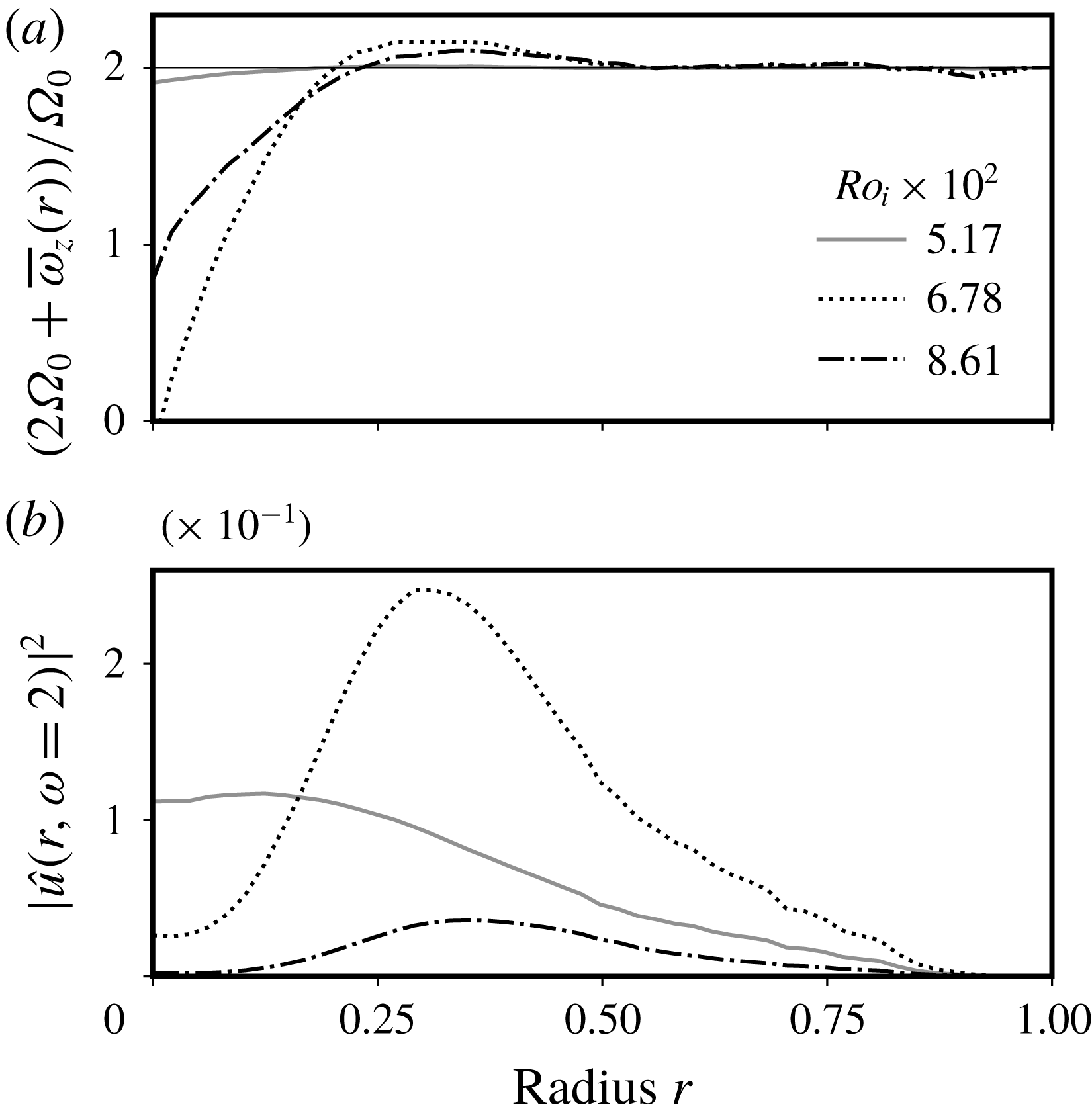
(a) Total vertical vorticity $2\unicode[STIX]{x1D6FA}_{0}+\overline{\unicode[STIX]{x1D714}}_{z}(r)$ of the fluid inside the ellipsoid as a function of the radius. (b) Local kinetic energy of the resonant mode at $\unicode[STIX]{x1D714}=2$ as a function of the radius. The energy is normalised by $(Ro_{i}a\unicode[STIX]{x1D6FA}_{0})^{2}$ and the radius by $a$ .

As may be noticed from the previous results, one of the striking consequences of the emergence of a strong geostrophic anticyclone is the loss of the numerous and well-defined triadic resonances detailed in the previous paragraph. The blurring of triadic resonances by geostrophic vortices is a well-known feature of randomly forced rotating turbulence: advection of inertial waves by these slowly evolving modes Doppler shifts their frequencies and forces them out of resonant interaction (Campagne et al. Reference Campagne, Gallet, Moisy and Cortet2014; Oks et al. Reference Oks, Mininni, Marino and Pouquet2017). Nevertheless, the present case is different from usual rotating turbulence since energy is only supplied to the system through a pair of inertial modes via the elliptical instability resonance. In addition, the vortex is persistent and drastically changes the local rotation rate of the fluid at the centre of the ellipsoid.

Figure 16.

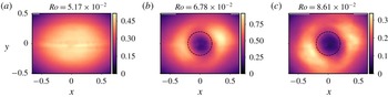
Norm of the velocity of the resonant wave extracted by temporal filtering of the saturation field below (a) and above (b,c) the threshold of the secondary transition on the geostrophic anticyclone. The dashed circle shows the radius at which the global vorticity is always below $2\unicode[STIX]{x1D6FA}_{0}$ , i.e.  $r/a\sim 0.2$ (see figure 15). The colour scale gives the norm of the velocity normalised by $Ro_{i}a\unicode[STIX]{x1D6FA}_{0}$ .

To better quantify the reaction of the waves to the existence of the strong anticyclone, we first consider the total vertical vorticity $2\unicode[STIX]{x1D6FA}_{0}+\overline{\unicode[STIX]{x1D714}}_{z}(r)$ , which is shown in figure 15, and where $\overline{\unicode[STIX]{x1D714}}_{z}$ is determined with (6.3). There exists a radius below which the global vorticity remains significantly below $2\unicode[STIX]{x1D6FA}_{0}$ , at the core of the anticyclonic vortex. Once the secondary transition develops, the core of the anticyclone cannot sustain the resonant mode at $\unicode[STIX]{x1D714}=2$ since the maximal frequency cannot exceed the total vertical vorticity. As a consequence, the radial structure of the resonant mode, which is constantly excited by the elliptical instability, changes as the secondary transition develops. This is illustrated in figures 15 and 16, where it appears clearly that the central amplitude of the resonant mode drops as the anticyclone emerges. Moreover, the spatial area affected by the drop in amplitude corresponds to the typical size of the vortex.

To conclude, the growth of the secondary transition alters the spatial structure of the resonant modes. The strong anticyclone that emerges significantly alters the global vorticity, and hence the structure of inertial modes. If they still exist, triadic resonances cannot be the same compared to the low forcing case as the structure of the modes has to account for the differential rotation introduced by the geostrophic flow.