

1. Introduction
Waves are ubiquitous in rotating and stratified fluids and participate in the dynamics of a very large variety of geophysical and astrophysical flows. In addition to transporting momentum, they are expected to be involved in mixing and dissipation processes. Of special interest are the viscous harmonic wave beams that are created from critical surfaces and boundary singularities because they are very thin and possess a universal transverse structure (Moore & Saffman Reference Moore and Saffman1969; Thomas & Stevenson Reference Thomas and Stevenson1972; Le Dizès & Le Bars Reference Le Dizès and Le Bars2017). The goal of the present article is to analyse the reflection of such beams on a flat boundary in order to understand how second-harmonic and meanflow corrections are created during the reflection process.
In the ocean, the tidal motion of water on submarine topography is an important source of waves (Wunsch Reference Wunsch1975). Supercritical topographies, that is, topographies steeper than the direction of propagation of the waves, are of particular interest because they are known to create strong concentrated beams. These beams and their role in tidal conversion have been studied experimentally (Zhang, King & Swinney Reference Zhang, King and Swinney2007; King, Zhang & Swinney Reference King, Zhang and Swinney2009; Echeverri & Peacock Reference Echeverri and Peacock2010) as well as theoretically (Llewellyn Smith & Young Reference Llewellyn Smith and Young2003; StLaurent etal. Reference St Laurent, Stringer, Garrett and Perrault-Joncas2003; Balmforth & Peacock Reference Balmforth and Peacock2009). Similar concentrated wave beams are also found in rotating fluids (Kerswell Reference Kerswell1995; Le Dizès & Le Bars Reference Le Dizès and Le Bars2017). They have mainly been studied in spherical geometries (Calkins etal. Reference Calkins, Noir, Eldredge and Aurnou2010; Koch etal. Reference Koch, Harlander, Egbers and Hollerbach2013; Cébron etal. Reference Cébron, Laguerre, Noir and Schaeffer2019; Lin & Noir Reference Lin and Noir2020) in the context of planetary applications (Le Bars, Cébron & Le Gal Reference Le Bars, Cébron and Le Gal2015). These wave beams are the temporal equivalent of the thin shear layers found at the periphery of Taylor–Proudman columns between differentially rotating discs or spheres (Proudman Reference Proudman1956; Stewartson Reference Stewartson1966). They have been the subject of works by Kerswell (Reference Kerswell1995), Walton (Reference Walton1975), Tilgner (Reference Tilgner2000) and Le Dizès (Reference Le Dizès2015) among others. Moore & Saffman (Reference Moore and Saffman1969) and Thomas & Stevenson (Reference Thomas and Stevenson1972) found independently for a rotating fluid and a stratified fluid, respectively, a self-similar viscous solution describing such a wave beam. These solutions were further studied and used by Peat (Reference Peat1978), Tabaei & Akylas (Reference Tabaei and Akylas2003), Voisin (Reference Voisin2003), Cortet, Lamriben & Moisy (Reference Cortet, Lamriben and Moisy2010) and Machicoane etal. (Reference Machicoane, Cortet, Voisin and Moisy2015). In Le Dizès & Le Bars (Reference Le Dizès and Le Bars2017), it was shown that these self-similar solutions are able to describe the wave beams that are created at the edge of a librating disc and at the critical latitude of a librating sphere in an open domain.
As soon as the domain is closed, the problem becomes more complex as beams reflect on boundaries. Depending on the geometry, concentrated beams can then also be formed as the result of a focusing process on an attractor (Maas etal. Reference Maas, Benielli, Sommeria and Lam1997; Rieutord, Georgeot & Valdettaro Reference Rieutord, Georgeot and Valdettaro2001; Grisouard, Staquet & Pairaud Reference Grisouard, Staquet and Pairaud2015; Beckebanze etal. Reference Beckebanze, Brouzet, Sibgatullin and Maas2018).
The reflection process of a wave beam has been documented (e.g. Phillips Reference Phillips1966). In contrast to a beam of light, a wave beam conserves its angle of propagation with respect to the direction of stratification or of the rotation axis. The beam structure is also expected to be conserved during the reflection process (Kistovich & Chashechkin Reference Kistovich and Chashechkin1994) except in thecritical situation where the boundary is aligned with the direction of propagation of the reflected beam (Dauxois & Young Reference Dauxois and Young1999). A viscous correction is also created during the reflection process that was first calculated by Beckebanze etal. (Reference Beckebanze, Brouzet, Sibgatullin and Maas2018).
Although a plane wave is known to be generically unstable by triadic resonance (Davis & Acrivos Reference Davis and Acrivos1967; Staquet & Sommeria Reference Staquet and Sommeria2002), a thin wave beam is less sensitive to such an instability (McEwan & Plumb Reference McEwan and Plumb1977; Dauxois etal. Reference Dauxois, Joubaud, Odier and Venaille2018). Moreover, it is also very weakly affected by nonlinear effects (Tabaei & Akylas Reference Tabaei and Akylas2003). Nonlinearities seem to be created mainly when two beams interact (Lamb Reference Lamb2004). This interaction process has been analysed theoretically by Tabaei, Akylas & Lamb (Reference Tabaei, Akylas and Lamb2005) and Jiang & Marcus (Reference Jiang and Marcus2009) in order to determine the amplitude and direction of propagation of nonlinearly generated waves. The case of a reflected beam is a particular case because the interacting beams have the same frequency. The first-order interaction therefore creates meanflow and second-harmonic corrections. In two dimensions, the meanflow correction tends to remain localized (Tabaei etal. Reference Tabaei, Akylas and Lamb2005) so many works have focused on the second-harmonic wave beam generated during the reflection process (Peacock & Tabaei Reference Peacock and Tabaei2005; Gostiaux etal. Reference Gostiaux, Dauxois, Didelle, Sommeria and Viboud2006; Rodenborn etal. Reference Rodenborn, Kiefer, Zhang and Swinney2011). Yet, non-local meanflow corrections could a priori be created in a stratified fluid, or a rotating fluid. In a stratified fluid, they take the form of horizontal layers. Bretherton (Reference Bretherton1969), Bordes etal. (Reference Bordes, Venaille, Joubaud, Odier and Dauxois2012) and Kataoka & Akylas (Reference Kataoka and Akylas2015) have shown they are amplified by three-dimensional effects. In a rotating fluid, they take the form of columnar flows. They seem to be generated by the nonlinear interaction occurring in the viscous boundary layer. They have been documented for precession (Busse Reference Busse1968; Hollerbach & Kerswell Reference Hollerbach and Kerswell1995; Noir, Jault & Cardin Reference Noir, Jault and Cardin2001), libration (Busse Reference Busse2010; Sauret etal. Reference Sauret, Cébron, Morize and Le Bars2010; Sauret & Le Dizès Reference Sauret and Le Dizès2013; Lin & Noir Reference Lin and Noir2020) and tides (Tilgner Reference Tilgner2007; Morize etal. Reference Morize, Le Bars, Le Gal and Tilgner2010; Favier etal. Reference Favier, Barker, Baruteau and Ogilvie2014).
In the present paper, we consider the generic situation of an axisymmetric (or two-dimensional) oscillating viscous beam, described by the self-similar solution of Moore & Saffman (Reference Moore and Saffman1969) and Thomas & Stevenson (Reference Thomas and Stevenson1972), impacting an axisymmetric (or planar) surface in a stratified and rotating fluid. Our objective is to analyse the weakly nonlinear structure of the solution generated during the reflection process. More specifically, we provide the scalings and the equations governing the meanflow and second-harmonic corrections in the limit of small Ekman numbers.
The paper is organized as follows. In § 2, we provide the theoretical framework and describe the reflection process of the self-similar wave beam solution. We show that a viscous correction is created during the reflection. The Reynolds stress responsible for the generation of a second-harmonic and of a meanflow correction is also discussed in this section. In § 3, we analyse the second-harmonic correction while § 4 is devoted to the meanflow correction. The structure of the meanflow correction is found to be particular when the fluid is non-rotating or non-stratified. These cases are treated in §§ 4.2 and 4.3. The results are briefly summarized in § 5 and compared to those of other works in § 6.
2. Framework
We consider an incompressible viscous fluid, rotating around an axis  $Ox$ with an angular velocity
 $\Omega$ and stably stratified along this axis with a constant buoyancy frequency
 $N$. The fluid is characterized by a kinematic viscosity
 $\nu$ and a diffusivity
 $\kappa$. In the rotating frame, the velocity field
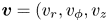 ${{\boldsymbol {v}}}=(v_r,v_\phi ,v_z$), the pressure
 $p$ and the buoyancy
 $b$ of the fluid perturbations are governed, under the Boussinesq approximations, by the equations
 \begin{gather} \frac{\textrm{D}{{\boldsymbol{v}}}}{\textrm{D}t} + 2\Omega {\boldsymbol{e_z}}\times{{\boldsymbol{v}}} = - \boldsymbol{\nabla} p - b {\boldsymbol{e_z}} + \nu {\nabla}^{2} {{\boldsymbol{v}}}, \end{gather}
 \begin{gather} \boldsymbol{\nabla} \boldsymbol{\cdot} {{\boldsymbol{v}}}=0, \end{gather}
 \begin{gather} \frac{\textrm{D}b}{\textrm{D}t} = N^{2} v_z + \kappa {\nabla}^{2} b, \end{gather}
where  $\textrm {D}/\textrm {D}t=(\partial /\partial t + {{\boldsymbol {v}}}\boldsymbol{\cdot} \boldsymbol {\nabla })$. Vanishing buoyancy and no-slip boundary conditions are assumed on solid boundaries.
We consider a thin oscillating wave beam in the form of an oscillating viscous internal shear layer. Its frequency  $\omega$ is related to the angle
 $\theta$ of propagation with respect to the horizontal plane by the relation
 \begin{equation} \omega^{2} = N^{2} \sin^{2}\theta + 4 \Omega^{2} \cos\theta^{2}. \end{equation}
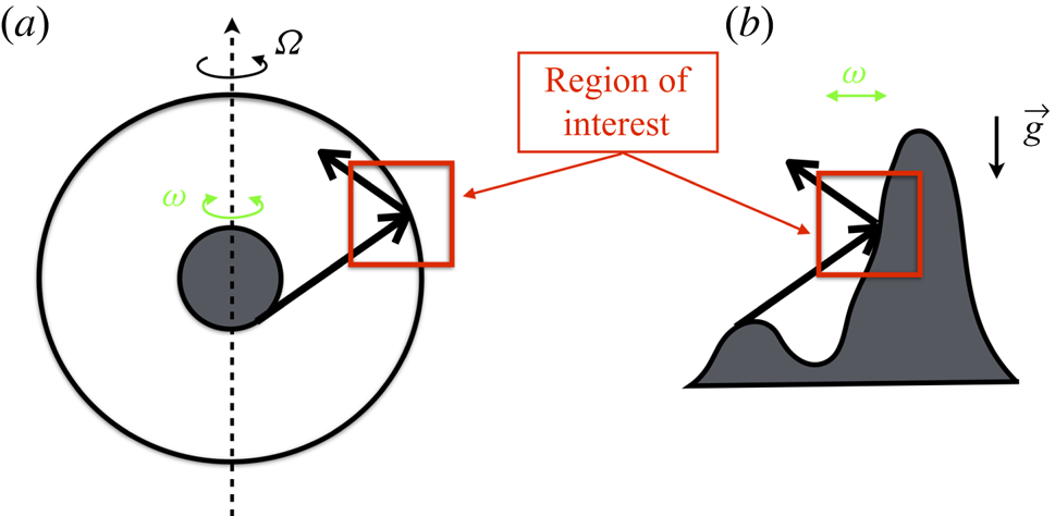
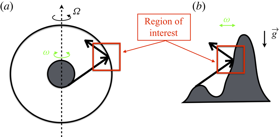
We consider a generic case for which  $0<\theta < {\rm \pi} /2$. As explained in the introduction, these internal shear layers are generated from oscillating objects or supercritical topographies in typical situations illustrated in figure 1. In this work, we are interested in the reflection of such a wave beam on an axisymmetric boundary making an angle
 $\alpha$ with respect to the horizontal plane. Our objective is to quantify the nonlinear corrections which are created during the reflection process. The presentation is provided for an axisymmetric beam in a cylindrical geometry but the same analysis can be done if the beam possesses another azimuthal symmetry, or if the beam and the boundary have a planar geometry.
Sketches of typical applications.  $(a)$ Reflection on an outer boundary of a wave beam generated by the libration of an inner core.
 $(b)$ Reflection on a mountain of a wave beam generated by a tidal wave on a supercritical topography.
2.1. Incident beam structure
The incident beam is assumed to be described by the similarity solution of Moore & Saffman (Reference Moore and Saffman1969) and Thomas & Stevenson (Reference Thomas and Stevenson1972).
Using the notation introduced in Le Dizès & Le Bars (Reference Le Dizès and Le Bars2017), this harmonic solution can be written as  ${{\boldsymbol {X}}} ^{(i)} = {\rm Re} (({{\boldsymbol {v}}}^{(i)},b^{(i)},p^{(i)}) \textrm {e}^{-{\textrm {i}} \omega t})$, where the velocity
 $v_{\parallel }^{(i)}$ along the direction of propagation, the azimuthal velocity
 $v_{\phi }^{(i)}$ and the buoyancy
 $b^{(i)}$ are all proportional to
 \begin{equation} H_{\mu}(x_{\perp}^{(i)},x_\parallel^{(i)},r) = \frac{1}{\sqrt{r} \left(x_\parallel^{(i)}\right)^{\mu /3}} {\boldsymbol{h_{\mu }}}\left(\frac{x_\perp^{(i)}}{\left(L_d^{2} x_\parallel^{(i)}\right)^{1/3}}\right) \end{equation}
with
 \begin{equation} v_{\parallel}^{(i)}= \varepsilon^{(i)} H_{\mu},\quad v_{\phi}^{(i)} = -\frac{2\Omega{\textrm{i}} \cos\theta}{\omega} \varepsilon^{(i)} H_{\mu},\quad b^{(i)} = \frac{ N^{2} {\textrm{i}} \sin \theta}{\omega} \varepsilon^{(i)} H_{\mu}. \end{equation}
In (2.3),  $r$ is the radial coordinate and
 $x_\parallel ^{(i)}$ and
 $x_\perp ^{(i)}$ are the coordinates parallel and normal to the direction of propagation of the incident wave beam in the
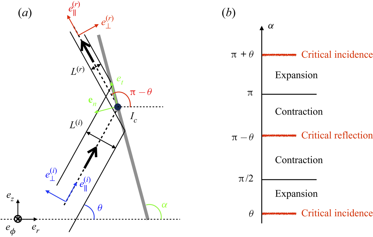
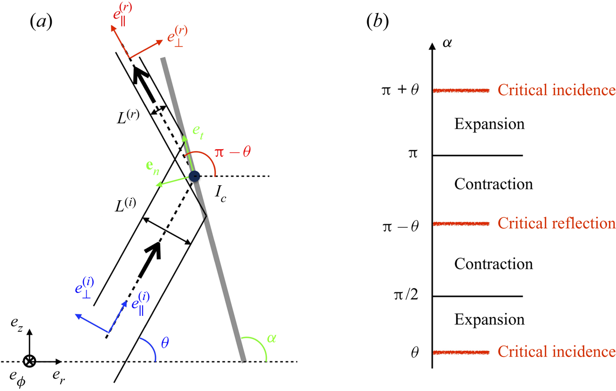
 $(r,z)$ plane (see figure 2
 $a$).
Reflection process.  $(a)$ Definition of the coordinate systems for
 $0 < \theta < \alpha {\rm \pi} -\theta$. Here the reflected beam is contracted because
 ${\rm \pi} /2<\alpha < {\rm \pi} -\theta$. The relationships between the various coordinate systems are provided in appendix A.
 $(b)$ Characteristic of the reflection process according to
 $\alpha$ (assuming
 $0<\theta <{\rm \pi} /2$).
The function  ${\boldsymbol {h_{\mu }}}$ is given by
 \begin{equation} {\boldsymbol{h_{\mu }}}(\zeta) = \frac{\textrm{e}^{-{\textrm{i}} \mu {\rm \pi}/2}}{(\mu -1)!} \int_0^{+\infty} \textrm{e}^{{\textrm{i}}p \zeta - p^{3}} p^{\mu -1}\, \textrm{d}p. \end{equation}
The index  $\mu$ characterizes the nature of the singularity which has given birth to the beam (Moore & Saffman Reference Moore and Saffman1969; Thomas & Stevenson Reference Thomas and Stevenson1972). For instance, an axisymmetric Dirac source is known to be associated with an index
 $\mu =1$ (Tilgner Reference Tilgner2000; Le Dizès Reference Le Dizès2015). Stronger singularities associated with larger values of
 $\mu$ can also be found. Le Dizès & Le Bars (Reference Le Dizès and Le Bars2017) demonstrated that the singularity associated with the critical latitude on a sphere gives rise to an index
 $\mu = 5/4$ (this situation is illustrated in figure 1
 $a$). Expression (2.4a--c) is also encountered in the far field of any localized source (Voisin Reference Voisin2003). In that case, the index
 $\mu$ characterizes the multipole order of the source (Machicoane etal. Reference Machicoane, Cortet, Voisin and Moisy2015); it is an integer in two dimensions, with
 $\mu =1$ for a dipole, but a half-integer in three dimensions, with
 $\mu =3/2$ for a dipole (Voisin Reference Voisin2003).
The constant  $L_d$ is given by
 \begin{equation} L_d^{2}= \frac{ N^{2}\sin^{2}\theta (\nu +\kappa) + 8 \Omega^{2} \nu \cos^{2}\theta}{2 \sin\theta\cos\theta (4 \Omega^{2}-N^{2}) \omega}. \end{equation}
Its norm defines a characteristic diffusion scale. In the non-stratified case ( $N=0$),
 $L_d^{2}= \nu /(2\Omega \sin \theta )$. In the non-rotating case (
 $\Omega =0$),
 $L_d^{2}= -(\nu +\kappa )/(2 N \cos \theta )$. When
 $L_d^{2}<0$, the quantity
 $(L_d^{2} x_\parallel ^{(i)})^{1/3}$ in (2.3) is defined as
 $-|L_d^{2} x_\parallel ^{(i)} |^{1/3}$.
The beam gets wider and wider as it propagates. We consider its characteristics at a typical distance  $l_c= x_{\parallel c}^{(i)}$ from its source. If we use a characteristic frequency
 $f_c$ (say
 $\max (2 \Omega ,N)$) and define the Ekman number by
 \begin{equation} E=\frac{\nu}{f_c l_c^{2}}, \end{equation}
the characteristic width of the beam is given by
 \begin{equation} L^{(i)} = E^{1/3} \Lambda l_c, \end{equation}
where  $\Lambda$ is a positive dimensionless number given by
 \begin{equation} \Lambda= \left| \frac{ N^{2}f_c\sin^{2}\theta (1 +{Pr}^{-1}) + 8 \Omega^{2} f_c\cos^{2}\theta}{2 \sin\theta\cos\theta (4 \Omega^{2}-N^{2}) \omega} \right|^{1/3}, \end{equation}
in which  ${Pr}= \nu /\kappa$ is the Prandtl number.
In the following, we assume that  $E\ll 1$ and that
 $\Lambda$ is neither zero nor infinite. The Prandtl number
 ${Pr}$ is assumed to be a fixed non-zero constant. The beam is therefore thin with a width scaling as
 $E^{1/3}$. This similarity solution is a leading-order approximation of a viscous solution in the limit
 $E\rightarrow 0$. The pressure
 $p^{(i)}$ and the normal velocity
 $v_\perp ^{(i)}$ are
 $O(E^{1/3})$ as the first-order correction to the similarity solution.
Note that the present similarity solution is a special case of a general expression of the form
 \begin{equation} v_\parallel = \frac{1}{\sqrt{r}} \int_{0}^{+\infty} G(k) \exp\left({{\textrm{i}} \epsilon_o k x_{\perp}/L^{(i)}}\right) \exp\left({- k^{3} x_{\parallel} /l_c}\right)\,\textrm{d}k, \end{equation}
which describes a viscous beam propagating in the direction of positive  $x_{\parallel }$. For our similarity solution,
 $G(k)= \varepsilon ^{(i)} \textrm {e}^{-{\textrm {i}} \mu {\rm \pi} /2} k^{\mu -1}/(\mu -1)!$. With the frame convention shown in figure 2
 $(a)$, the parameter
 $\epsilon _o$ is equal to
 $1$ if
 $N<2 \Omega$ and to
 $-1$ if
 $N>2 \Omega$. The singular case
 $N=2 \Omega$ is not considered in the present work.
In the following, all the spatial and temporal variables are assumed to have been non-dimensionalized using  $l_c$ and
 $f_c$.
2.2. Reflection on an inclined boundary
After having covered a distance  $l_c$, the incident beam reaches an inclined boundary and is reflected as illustrated in figure 2
 $(a)$. This reflection process is analogous to that described by Phillips (Reference Phillips1966) for a plane wave in a non-rotating fluid, and further analysed by Kistovich & Chashechkin (Reference Kistovich and Chashechkin1994) and Tabaei etal. (Reference Tabaei, Akylas and Lamb2005). According to the boundary inclination angle
 $\alpha$, the beam is expected to expand or contract (see figure 2
 $b$). As in Kistovich & Chashechkin (Reference Kistovich and Chashechkin1994), we assume that the beam keeps its self-similar structure (2.3) with new variables
 $x_{\parallel }^{(r)}$ and
 $x_\perp ^{(r)}$ associated with the direction of the reflected beam. We consider the situation illustrated in figure 2
 $(a)$ where
 $\theta ^{(i)}= \theta$ and
 $\theta ^{(r)}= {\rm \pi} -\theta$ and look for a solution
 ${{\boldsymbol {X}}} ^{(r)} = {\rm Re} (({{\boldsymbol {v}}}^{(r)},b^{(r)},p^{(r)}) \textrm {e}^{-{\textrm {i}} \omega t})$ with
 \begin{equation} v_{\parallel}^{(r)}= \varepsilon^{(r)} H_{\mu},\quad v_{\phi}^{(r)} = \frac{2\Omega{\textrm{i}} \cos\theta}{\omega} \varepsilon^{(r)} H_{\mu},\quad b^{(r)} = \frac{ N^{2} {\textrm{i}} \sin \theta}{\omega} \varepsilon^{(r)} H_{\mu}. \end{equation}
The reflected beam amplitude  $\varepsilon ^{(r)}$ and the value
 $x_{\parallel c}^{(r)}$ of
 $x_{\parallel }^{(r)}$ at the impact point
 $I_c(r_c,z_c)$ should be chosen such that the sum of incident and reflected beams satisfies the condition of non-penetrability on the surface. To apply this condition, it is convenient to introduce local variables tangential and normal to the boundary (see figure 2a):
 \begin{equation} x_t= \cos\alpha (r-r_c) + \sin\alpha (z-z_c),\quad x_n= -\sin\alpha (r-r_c) + \cos\alpha (z-z_c), \end{equation}
such that the condition  $v_n(x_n=0)=0$ gives
 \begin{align} & -\sin(\alpha -\theta) \varepsilon^{(i)} H_{\mu}(\sin(\alpha-\theta) x_t, x_{\parallel _c}^{(i)},r_c)\nonumber\\ &\qquad + \sin(\alpha +\theta) \varepsilon^{(r)} H_{\mu} (\sin(\alpha + \theta) x_t,x_{\parallel _c}^{(r)},r_c ) =0. \end{align}
This equation is satisfied if and only if
 \begin{equation} \frac{x_{\parallel c}^{(i)}}{x_{\parallel c}^{(r)}} = K^{3},\quad \frac{\varepsilon^{(i)}}{\varepsilon^{(r)}} =K^{\mu -1}, \end{equation}
with
 \begin{equation} K= \frac{\sin(\alpha -\theta)}{\sin(\alpha +\theta)}. \end{equation}
Equations (2.14) were already obtained by Kistovich & Chashechkin (Reference Kistovich and Chashechkin1994). They noted that the reflected beam can be interpreted as a beam generated by a virtual source of the same nature as the incident beam but located at a distance  $x_{\parallel c}^{(r)}$ from the reflection point given by (2.14). Close to the impact point, the width of the reflected beam is given by
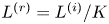 $L^{(r)} = L^{(i)}/K$. The coefficient
 $K$ is therefore the contraction factor of the reflected beam. We can indeed check that the reflected beam expands (
 $0<K<1$) for
 $\theta <\alpha <{\rm \pi} /2$ and contracts (
 $K>1$) for
 ${\rm \pi} /2<\alpha < {\rm \pi} - \theta$ in agreement with figure 2(b). This formula for the contraction factor is not new and is related to the wavelength contraction factor that a plane wave experiences at reflection (Phillips Reference Phillips1966).
In a region of order  $E^{1/3}$ around the impact point that we call the interaction region, a compact expression of the total harmonic field composed of the incident and reflected beams can be obtained. If we redefine
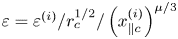 $\varepsilon = \varepsilon ^{(i)}/r_c^{1/2}/\left (x_{\parallel c}^{(i)}\right )^{\mu /3}$, and introduce the local variables
 $\tilde {r} = (r-r_c)/E^{1/3}$ and
 $\tilde {z} =(z -z_c)/E^{1/3}$, we can write the leading-order expression of the velocity and buoyancy fields in the interaction region as
 \begin{equation} ({{\boldsymbol{v}}}, b) \sim \varepsilon \left(\boldsymbol{\tilde{v}}_0, \tilde{b}_0\right) = \varepsilon \left(\boldsymbol{\tilde{v}}_0^{(i)}+ \boldsymbol{\tilde{v}}_0^{(r)}, \tilde{b}_0^{(r)} + \tilde{b}_0^{(i)}\right), \end{equation}
 \begin{gather} {\tilde{v}}_{0r} = \cos \theta \left( \tilde{h}_{\mu}^{(i)} - \tilde{h}_{\mu}^{(r)} \right), \end{gather}
 \begin{gather} {\tilde{v}}_{0\phi } = - \frac{2 \Omega \cos\theta }{\omega} \left( \tilde{h}_{\mu}^{(i)} - \tilde{h}_{\mu}^{(r)} \right), \end{gather}
 \begin{gather} {\tilde{v}}_{0z} = \sin \theta \left( \tilde{h}_{\mu}^{(i)} + \tilde{h}_{\mu}^{(r)} \right), \end{gather}
 \begin{gather} \tilde{b}_0= {\textrm{i}} \frac{N^{2} \sin \theta}{\omega} \left( \tilde{h}_{\mu}^{(i)} + \tilde{h}_{\mu}^{(r)} \right) \end{gather}
and
 \begin{equation} \tilde{h}_{\mu }^{(i)} = {\boldsymbol{h_{\mu }}}\left(\frac{-\sin\theta \tilde{r} + \cos \theta \tilde{z} }{\Lambda} \right) ,\quad \tilde{h}_{\mu }^{(r)} = K {\boldsymbol{h_{\mu }}}\left(K\frac{\sin\theta \tilde{r} + \cos \theta \tilde{z} }{\Lambda} \right). \end{equation}
Note that in terms of local boundary layer variables 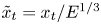 $\tilde {x}_t=x_t/E^{1/3}$ and
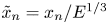 $\tilde {x}_n=x_n/E^{1/3}$,
 $\tilde {h}_{\mu }^{(i)}$ and
 $\tilde {h}_{\mu }^{(r)}$ can also be written as
 \begin{gather} \tilde{h}_{\mu}^{(i)}= {\boldsymbol{h_{\mu }}} \left(\frac{\sin(\alpha-\theta)}{\Lambda}(\tilde{x}_t + \cot (\alpha -\theta) \tilde{x}_n ) \right) , \end{gather}
 \begin{gather} \tilde{h}_{\mu} ^{(r)} = K {\boldsymbol{h_{\mu }}}\left(\frac{\sin(\alpha-\theta)}{\Lambda}\left(\tilde{x}_t + \cot (\alpha +\theta) \tilde{x}_n \right) \right) , \end{gather}
and the tangential and normal velocity components read
 \begin{gather} \tilde{v}_{0t} = \cos ( \alpha-\theta) \tilde{h}_{\mu}^{(i)} - \cos(\alpha+\theta) \tilde{h}_{\mu} ^{(r)} , \end{gather}
 \begin{gather} \tilde{v}_{0n} = -\sin ( \alpha-\theta) \tilde{h}_{\mu}^{(i)} +\sin (\alpha+\theta) \tilde{h}_{\mu} ^{(r)}. \end{gather}
It is worth mentioning that the above solution is a leading-order approximation obtained by applying slip boundary conditions. This solution does not satisfy the vanishing buoyancy and no-slip boundary conditions. This means that a viscous/diffusive boundary layer is expected close to boundary. In the next subsection, we show that this viscous boundary layer is responsible for a viscous correction to the reflected beam. More precisely, we shall see that the reflected beam expands in the interaction region as
 \begin{equation} ({{\boldsymbol{v}}}^{(r)}, b^{(r)}) = \varepsilon \left[\left(\boldsymbol{\tilde{v}}_0^{(r)}, \tilde{b}_0^{(r)}\right) + E^{1/6} \left(\boldsymbol{\tilde{v}}_1^{(r)}, \tilde{b}_1^{(r)}\right) + O\left(E^{1/3}\right) \right], \end{equation}
whereas the incident beam is just
 \begin{equation} ({{\boldsymbol{v}}}^{(i)}, b^{(i)}) = \varepsilon \left[\left(\boldsymbol{\tilde{v}}_0^{(i)}, \tilde{b}_0^{(i)}\right) + O\left(E^{1/3}\right) \right]. \end{equation}
2.3. Viscous correction to the reflected beam
As long as the slope inclination is not critical, that is,  $\alpha$ is different from
 $\theta$ and
 ${\rm \pi} - \theta$, the width of the viscous boundary layer is
 $O(E^{1/2})$. In the viscous boundary layer, the relevant variables are the local tangent variable
 $\tilde {x}_t$ and the viscous boundary variable
 $\bar {x} _n = E^{-1/6}\tilde {x}_n = E^{-1/2} x_n$. The form of the solution can be obtained by expanding the leading-order expression (2.17) as
 $\tilde {x} _n \rightarrow 0$ using the viscous boundary variable. Using (2.20), we observe that
 $\tilde {v}_{0t}$,
 $\tilde {v}_{0\phi }$,
 $\tilde {b}_0$ remain
 $O(1)$ whereas
 $\tilde {v}_{0n}\sim \tilde {x}_n \partial _{\tilde {x}_n}\tilde {v}_{0n}(\tilde {x}_t,0) = E^{1/6} \bar {x}_n \partial _{\tilde {x}_n}\tilde {v}_{0n}(\tilde {x}_t,0)$ as
 $\tilde {x} _n \rightarrow 0$. It follows that one can look for a viscous boundary solution of the form
 \begin{gather} v_t = \varepsilon \big(\tilde{v}_{0t0}(\tilde{x}_t) + \bar{v}_{0t}(\tilde{x}_t,\bar{x}_n) \big) , \end{gather}
 \begin{gather} v_n= \varepsilon E^{1/6} \bar{v}_{1n}\left(\tilde{x}_t,\bar{x}_n\right), \end{gather}
 \begin{gather} v_\phi = \varepsilon \left(\tilde{v}_{0\phi 0}\left(\tilde{x}_t\right) + \bar{v}_{0\phi}\left(\tilde{x}_t,\bar{x}_n\right) \right) , \end{gather}
 \begin{gather} b = \varepsilon \left(\tilde{b}_{00}\left(\tilde{x}_t\right) + \bar{b}_{0}\left(\tilde{x}_t,\bar{x}_n\right)\right) , \end{gather}
 \begin{gather} p = \varepsilon E^{1/3} \left(\tilde{p}_{00}\left(\tilde{x}_t\right) + E^{1/6} \bar{p}_1\left(\tilde{x}_t,\bar{x}_n\right) \right), \end{gather}
where  $\tilde {v}_{0t0}$,
 $\tilde {v}_{0\phi 0}$,
 $\tilde {b}_{00}$ and
 $\tilde {p}_{00}$ are the expressions as
 $\tilde {x}_n$ goes to 0 of the leading-order solution in the interaction region. Only
 $\tilde {p}_0$ has not been provided above. Its exact expression will turn out not to be necessary for the analysis.
The governing equations reduce to
 \begin{gather} -{\textrm{i}} \omega \bar{v}_{0t} -2 \Omega \bar{v}_{0\phi} \cos\alpha - \bar{b}_0 \sin\alpha - \displaystyle\frac{\partial ^{2}{\bar{v}_{0t}}}{\partial {\bar{x}_n}^{2}} =0 , \end{gather}
 \begin{gather} -{\textrm{i}} \omega \bar{v}_{0\phi} +2 \Omega \bar{v}_{t 0} \cos\alpha - \displaystyle\frac{\partial ^{2}{\bar{v}_{0\phi}}}{\partial {\bar{x}_n}^{2}} = 0 , \end{gather}
 \begin{gather} 2 \Omega \bar{v}_{0\phi} \sin\alpha - \bar{b}_0 \cos\alpha + \displaystyle\frac{\partial {\bar{p}_1}}{\partial {\bar{x}_n}} =0, \end{gather}
 \begin{gather} -{\textrm{i}} \omega \bar{b}_{0} -2 \Omega \bar{v}_{0\phi} \cos\alpha - N^{2} \bar{v}_{0t} \sin\alpha - \frac{1}{{Pr}} \displaystyle\frac{\partial ^{2}{\bar{b}_{0}}}{\partial {\bar{x}_n}^{2}} = 0 , \end{gather}
 \begin{gather} \displaystyle\frac{\partial {\bar{v}_{1n}}}{\partial {\bar{x}_n}} + \displaystyle\frac{\partial {\left(\tilde{v}_{0t0} +\bar{v}_{0t}\right)}}{\partial {\tilde{x}_t}} = 0 , \end{gather}
which give
 \begin{align} & \left[\left( {\textrm{i}} \omega + \displaystyle\frac{\partial ^{2}{}}{\partial {\bar{x}_n}^{2}} \right)^{2}\left( {\textrm{i}} \omega + \displaystyle\frac{1}{{Pr}}\displaystyle\frac{\partial ^{2}{}}{\partial {\bar{x}_n}^{2}} \right) + 4\Omega^{2} \cos^{2}\alpha \left( {\textrm{i}} \omega + \displaystyle\frac{1}{{Pr}}\displaystyle\frac{\partial ^{2}{}}{\partial {\bar{x}_n}^{2}} \right) \right.\nonumber\\ &\qquad \left. + N^{2} \sin^{2}\alpha \left( {\textrm{i}} \omega + \displaystyle\frac{\partial ^{2}{}}{\partial {\bar{x}_n}^{2}} \right) \right] \bar{v} _{0t} =0. \end{align}
Among the six independent solutions, three correspond to exponentially decreasing solutions of the form  $\textrm {e}^{-\lambda _j \bar {x}_n}$,
 $j=1,2,3$ with
 $\mathrm {Re}(\lambda _j) >0$. The solution for
 $\bar {v}_{0t}$ can then be written as
 $\bar {v}_{0t} =\sum _{j=1}^{3} \bar {a}_j(\tilde {x}_t) \textrm {e}^{-\lambda _j\bar {x}_n}$, which gives similar expressions for
 $\bar {v}_{0\phi }$ and
 $\bar {b}_{0}$ using (2.24a), (2.24b) and (2.24d). The conditions that
 $v_{t}$,
 $v_\phi$ and
 $b$ vanish at
 $\bar {x}_n=0$ then provide the functions
 $\bar {a}_j$,
 $j=1,2,3$ as linear combinations of
 $\tilde {v}_{0t0}$,
 $\tilde {v}_{0\phi 0}$ and
 $\tilde {b}_{00}$. Note that if
 ${Pr} =\infty$, (2.25) is of fourth order. There are then two unknown functions, which are obtained by applying the boundary conditions at
 $\bar {x} _n=0$ on
 $v_{t}$ and
 $v_\phi$ only.
To get  $\bar {v}_{1n}$, we use (2.24e) which gives
 \begin{equation} \bar{v}_{1n} = -\tilde{v}_{0t0}'(\tilde{x}_t) \bar{x}_n - \sum_{j=1}^{3} \bar{a}'_j(\tilde{x}_t) \frac{1 - \textrm{e}^{-\lambda_j \bar{x}_n}}{\lambda_j}. \end{equation}
The first term automatically matches the expression of the normal velocity in the interaction region as  $\tilde {x}_n\rightarrow 0$. It is the second term that gives the viscous correction for which we are looking. As
 $\bar {x}_n \rightarrow \infty$, this term tends to a function
 $\bar {u}_{1n}^{\infty }(\tilde {x}_t)= - \sum _{j=1}^{3} \bar {a}'_j(\tilde {x}_t) /\lambda _j$ that should match a contribution in the interaction region. Using the fact that
 $\bar {a}_j(\tilde {x}_t)$,
 $j=1,2,3$ are a linear combination of
 $\tilde {v}_{0t0}$,
 $\tilde {v}_{0\phi 0}$ and
 $\tilde {b}_{00}$, they can be written as
 $C_j {\boldsymbol {h_{\mu }}}(\sin (\alpha -\theta ) \tilde {x}_t/\Lambda )$ (see (2.17) and (2.19)). It then immediately follows that
 \begin{equation} \bar{u}_{1n}^{\infty}(\tilde{x}_t)= C_{1n}^{\infty} {\boldsymbol{h_{\mu +1}}}( \sin(\alpha-\theta) \tilde{x}_t/\Lambda), \end{equation}
where  $C_{1n}^{\infty }$ is a complex constant. Such a normal flow can be matched in the interaction region to a solution of the same form as the reflected beam (2.11) by changing
 $\mu$ into
 $\mu +1$. More precisely, if we have (2.27), the viscous correction to the reflected beam would read in the interaction region as
 \begin{equation} \left( \begin{array}{@{}c@{}} v_{1r}^{(r)} \\ v_{1\phi}^{(r)} \\ v_{1z}^{(r)} \\ b_1^{(r)} \end{array} \right) = \varepsilon E^{1/6} C_{1n}^{\infty} \left( \begin{array}{@{}c@{}} \cos\theta \\ (2{\textrm{i}} \Omega / \omega) \cos\theta \\ \sin\theta \\ ({\textrm{i}}N^{2} /\omega) \sin\theta \end{array} \right) \tilde{h}_{\mu +1}^{(r)} , \end{equation}
where  $\tilde {h}_{\mu }^{(r)}$ has been defined in (2.19b). It is worth mentioning that this
 $O(E^{1/6})$ viscous correction is larger than the first viscous correction to the similarity solution describing the beam, which is
 $O(E^{1/3})$.
A viscous correction to the reflected beam was calculated by Beckebanze etal. (Reference Beckebanze, Brouzet, Sibgatullin and Maas2018) in the purely stratified case. By comparing their expression (6.9) with ours, one can see that both expressions are similar. They obtained that the spectral density of the viscous correction is  $k\hat {U}(k)$ if the spectral density of the incident beam is
 $\hat {U}(k)$ (our function
 $G(k)$ in (2.10)): this corresponds to the passage from
 ${\boldsymbol {h_{\mu }}}$ to
 ${\boldsymbol {h_{\mu +1}}}$ in our analysis.
2.4. Reynolds stress
In this section, our objective is to estimate the nonlinear terms  $\boldsymbol {v} \boldsymbol{\cdot} \boldsymbol {\nabla } \boldsymbol {v}$ and
 $\boldsymbol {v} \boldsymbol{\cdot} \boldsymbol {\nabla } b$, or Reynolds stress, that appear in the governing equations (2.1a)–(2.1c). Owing to the particular form of the similarity solution, it is straightforward to show that these terms are at most
 $O(\varepsilon ^{2})$ everywhere except close to the source, the rotation axis and the reflection point. As already mentioned, our interest is in a reflection point distinct from the beam source and the rotation axis.
In the interaction region, the two beams interact with each other, making the Reynolds stress of order  $\varepsilon ^{2} E^{-1/3}$. Simple expressions for the Reynolds stress can be obtained using (2.17a)–(2.17d) and (2.28). As expected, the Reynolds stress is composed of a steady and a second-harmonic part:
 \begin{equation} \boldsymbol{\mathcal{N}} = \boldsymbol{\mathcal{N}}^{(0)}+ \left(\boldsymbol{\mathcal{N}}^{(2)}\textrm{e}^{-2{\textrm{i}} \omega t} +\hbox{c.c.}\right), \end{equation}
where
 \begin{equation} \boldsymbol{\mathcal{N}}^{(0)} = \boldsymbol{v} \boldsymbol{\cdot} \boldsymbol{\nabla} \left( \begin{array}{@{}c@{}} v_r ^{*}\\ v_\phi^{*} \\ v_z ^{*}\\ b^{*} \end{array} \right) +\hbox{c.c.};\quad \boldsymbol{\mathcal{N}}^{(2)} = \boldsymbol{v}\boldsymbol{\cdot} \boldsymbol{\nabla} \left( \begin{array}{c} v_r \\ v_\phi \\ v_z \\ b \end{array} \right), \end{equation}
the superscript  $^{*}$ denoting the complex conjugate. The expressions of
 $\boldsymbol {\mathcal {N}}^{(0)}= \varepsilon ^{2}E^{-1/3}(\boldsymbol {\mathcal {N}}_0^{(0)} + E^{1/6}\boldsymbol {\mathcal {N}}_1^{(0)} + \cdots )$ and
 $\boldsymbol {\mathcal {N}}^{(2)} = \varepsilon ^{2}E^{-1/3}\boldsymbol {\mathcal {N}}_0^{(2)} + \cdots$ are given in appendix B.
2.5. Notation
We have introduced a number of notations that we shall use in the rest of the paper.
Whereas the harmonic solution is denoted without a superscript, the second-harmonic correction as well as the amplitude of the terms oscillating at a frequency  $2\omega$, such as the second-harmonic part of the Reynolds stress
 $\boldsymbol {\mathcal {N}}^{(2)}$, will be denoted with the superscript
 ${(2)}$. The meanflow correction and the steady terms such as
 $\boldsymbol {\mathcal {N}}^{(0)}$ will always be indicated by the superscript
 ${(0)}$.
The subscripts will be of three types. The letters and special characters  $\perp$ and
 $\parallel$ indicate the system of coordinates used for the velocity components. Three different systems of coordinates are used:
 $(r,\phi ,z)$ for the global cylindrical coordinate system,
 $(x_t,\phi ,x_n)$ for the boundary coordinate system and
 $(x_\parallel , \phi , x_\perp )$ for the beam-associated coordinate system (see figure 2a and appendix A for the relations between the coordinate systems). In this last case, the superscripts
 ${(i)}$,
 ${(r)}$,
 ${(2)}$ or
 ${(0)}$ indicate whether it corresponds to the incident, reflected, second-harmonic or steady beam. For the Reynolds stress, the subscript
 $b$ indicates the fourth component of the vector
 $\boldsymbol {\mathcal {N}}$.
The first subscript number is associated with the order of the expansion. The subscript  $0$ always indicates the leading-order expression; larger numbers correspond to higher-order terms ordered in decreasing amplitude order. A second subscript number
 $0$ or
 $\infty$ will exceptionally be used to indicate the value taken as one of the variables goes to zero or infinity.
The symbols placed above the characters correspond to the regions where the solution is considered:
(i) tilde (
 $\tilde {\ \ }$) for the interaction region;
(ii) overbar (
$\bar {\ \ }$) for the viscous boundary layer;(iii) check (
$\check {\ \ }$) for the $E^{4/9}$ viscous layer; and(iv) without symbol for the outer region, that is, in a beam region far from the interaction region.


For the spatial variables, the symbol will imply a particular rescaling with respect to the global outer variable, by  $E^{1/3}$ in the interaction region (i.e.
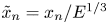 $\tilde {x}_n= x_n/E^{1/3}$,
 $\tilde {r}=(r-r_c)/E^{1/3}$, etc.), by
 $E^{1/2}$ in the viscous boundary layer for the normal variable (
 $\bar {x} = x_n/E^{1/2}$), by
 $E^{4/9}$ in the
 $E^{4/9}$ viscous layer for the normal variable (
 $\check {x}_n=x_n/E^{1/4}=\check {r} = (r-r_c)/E^{4/9}$ for a vertical boundary).
3. Second-harmonic correction
The second-harmonic Reynolds stress creates a second-harmonic correction  ${{\boldsymbol {X}}} ^{(2)} = {\rm Re} (({{\boldsymbol {v}}}^{(2)},b^{(2)},p^{(2)}) \textrm {e}^{-2{\textrm {i}} \omega t})$ that can be written in the interaction region as
 \begin{gather} v_r^{(2)} \sim \varepsilon^{2} E^{-1/3} \tilde{v}_{0r}^{(2)} (\tilde{r},\tilde{z}) , \end{gather}
 \begin{gather} v_\phi^{(2)} \sim \varepsilon^{2} E^{-1/3} \tilde{v}_{0\phi}^{(2)} (\tilde{r},\tilde{z}) , \end{gather}
 \begin{gather} v_z^{(2)} \sim \varepsilon^{2} E^{-1/3} \tilde{v}_{0z}^{(2)} (\tilde{r},\tilde{z}) , \end{gather}
 \begin{gather} b^{(2)} \sim \varepsilon^{2} E^{-1/3} \tilde{b}_0^{(2)} (\tilde{r},\tilde{z}) , \end{gather}
 \begin{gather} p^{(2)} \sim \varepsilon^{2} \tilde{p}_0^{(2)} (\tilde{r},\tilde{z}) , \end{gather}
where they satisfy
 \begin{gather} -2{\textrm{i}} \omega \tilde{v}_{0r}^{(2)} -2 \Omega \tilde{v}_{0\phi}^{(2)} + \displaystyle\frac{\partial {\tilde{p}_0^{(2)}}}{\partial {\tilde{r}}} = -\tilde{{\mathcal{N}}}_{0r}^{(2)} , \end{gather}
 \begin{gather} -2{\textrm{i}} \omega \tilde{v}_{0\phi}^{(2)} + 2 \Omega \tilde{v}_{0r}^{(2)} = -\tilde{{\mathcal{N}}}_{0\phi}^{(2)} , \end{gather}
 \begin{gather} -2{\textrm{i}} \omega \tilde{v}_{0z}^{(2)} + \tilde{b}_0^{(2)} + \displaystyle\frac{\partial {\tilde{p}_0^{(2)}}}{\partial {\tilde{z}}} = -\tilde{{\mathcal{N}}}_{0z}^{(2)}, \end{gather}
 \begin{gather} -2{\textrm{i}} \omega \tilde{b}_0^{(2)} -N^{2} \tilde{v}_{0z}^{(2)} = -\tilde{{\mathcal{N}}}_{0b}^{(2)} , \end{gather}
 \begin{gather} \displaystyle\frac{\partial {\tilde{v}_{0r}^{(2)}}}{\partial {\tilde{r}}} + \displaystyle\frac{\partial {\tilde{v}_{0z}^{(2)}}}{\partial {\tilde{z}}} =0. \end{gather}
These equations do not contain any viscous terms, which all come at higher orders. As seen below, these equations with a non-penetrability condition on the boundary completely define the leading order of the second-harmonic correction. This will allow us to say that the generation process of the second-harmonic correction is essentially inviscid.
The system (3.2) can be manipulated to give
 \begin{equation} (N^{2} - 4\omega^{2}) \displaystyle\frac{\partial {\tilde{v}_{0z}^{(2)}}}{\partial {\tilde{r}}} - (4 \Omega^{2} - 4 \omega^{2}) \displaystyle\frac{\partial {\tilde{v}_{0r}^{(2)}}}{\partial {\tilde{z}}} = -2 {\textrm{i}} \omega \frac{\partial^{2} (\tilde{h}_{\mu}^{(r)} \tilde{h}_{\mu}^{(i)})}{\partial \tilde{r} \partial \tilde{z}} \equiv {\mathcal{A}}^{(2)}. \end{equation}
Using (3.2e), we then get for  $\tilde {v}_{0r}^{(2)}$ and
 $\tilde {v}_{0z}^{(2)}$:
 \begin{equation} {\mathcal{L}}^{(2)} \tilde{v}_{0r}^{(2)} = -\displaystyle\frac{\partial {{\mathcal{A}}^{(2)}}}{\partial {\tilde{z}}},\quad {\mathcal{L}}^{(2)} \tilde{v}_{0z}^{(2)} = \displaystyle\frac{\partial {{\mathcal{A}}^{(2)}}}{\partial {\tilde{r}}} , \end{equation}
with
 \begin{equation} {\mathcal{L}}^{(2)} = (N^{2} - 4\omega^{2}) \displaystyle\frac{\partial ^{2}{}}{\partial {\tilde{r}}^{2}} + (4 \Omega^{2} - 4 \omega^{2}) \displaystyle\frac{\partial ^{2}{}}{\partial {\tilde{z}}^{2}} , \end{equation}
which also give for the tangential and normal components of the velocity:
 \begin{equation} {\mathcal{L}}^{(2)} \tilde{v}_{0t}^{(2)} = -\displaystyle\frac{\partial {{\mathcal{A}}^{(2)}}}{\partial {\tilde{x}_n}},\quad {\mathcal{L}}^{(2)} \tilde{v}_{0n}^{(2)} = \displaystyle\frac{\partial {{\mathcal{A}}^{(2)}}}{\partial {\tilde{x}_t}} , \end{equation}
where  ${\mathcal {L}}^{(2)}$ can also be written as
 \begin{align} & {\mathcal{L}}^{(2)} = (N^{2} \sin^{2}\alpha + 4 \Omega^{2} \cos^{2} \alpha - 4 \omega^{2}) \displaystyle\frac{\partial ^{2}{}}{\partial {\tilde{x}_n}^{2}} + (N^{2} \cos^{2}\alpha + 4 \Omega^{2} \sin^{2} \alpha - 4 \omega^{2}) \displaystyle\frac{\partial ^{2}{}}{\partial {\tilde{x}_t}^{2}}\nonumber\\ &\qquad\quad - \sin 2\alpha (N^{2} -4\Omega^{2}) \displaystyle\frac{\partial^{2}}{\partial \tilde{x}_t \partial \tilde{x}_n}. \end{align}
When  $2\omega$ is not within
 $2\Omega$ and
 $N$, (3.4a,b) and (3.6a,b) are elliptic equations: oscillations with respect to one variable are evanescent with respect to the other. In that case, we do not expect propagation outside the interaction region. The second-harmonic correction is localized in that region.
The interesting case is when  $2\omega$ is within
 $2\Omega$ and
 $N$. In other words, the second-harmonic frequency corresponds to an inertia–gravity frequency. In that case, there exists an angle
 $\theta _2$ (between 0 and
 ${\rm \pi} /2$) that satisfies
 \begin{equation} 4 \omega^{2} = N^{2} \sin^{2}\theta_2 + 4 \Omega^{2} \cos^{2}\theta_2, \end{equation}
which corresponds to a direction of propagation of perturbations of frequency  $2\omega$. The other directions of propagation are
 ${\rm \pi} -\theta _2$,
 ${\rm \pi} +\theta _2$ and
 $-\theta _2$. This angle can be used to write (3.7) as
 \begin{align} {\mathcal{L}}^{(2)} & = (N^{2} - 4\Omega^{2})\left( \sin(\alpha+ \theta_2) \displaystyle\frac{\partial {}}{\partial {\tilde{x}_n}} - \cos(\alpha+ \theta_2) \displaystyle\frac{\partial {}}{\partial {\tilde{x}_t}} \right)\nonumber\\ &\quad \times \left( \sin(\alpha- \theta_2) \displaystyle\frac{\partial {}}{\partial {\tilde{x}_n}} - \cos(\alpha- \theta_2) \displaystyle\frac{\partial {}}{\partial {\tilde{x}_t}} \right). \end{align}
As shown by Tabaei etal. (Reference Tabaei, Akylas and Lamb2005), a general solution to (3.6a,b) can then be obtained using Fourier transforms. For  $\tilde {v}_{0n}^{(2)}$, we get
 \begin{align} \tilde{v} _{0n}^{(2)} &=\int _{-\infty}^{+\infty} \exp\left({{\textrm{i}}k \left(\tilde{x}_t + \cot\left(\alpha - \theta_2\right) \tilde{x}_n\right) }\right)\nonumber\\ &\quad \times \left( A(k) + \int _{+\infty}^{\tilde{x}_n} \exp({-{\textrm{i}}k \cot(\alpha+ \theta_2)s}) {\mathcal{F}}(k,s)\,\textrm{d}s \right)\,\textrm{d}k\nonumber\\ &\quad + \int _{-\infty}^{+\infty} \exp\left({{\textrm{i}}k \left(\tilde{x}_t + \cot(\alpha +\theta_2) \tilde{x}_n\right) }\right)\nonumber\\ &\quad\times \left( B(k) - \int _{+\infty}^{\tilde{x}_n} \exp({-{\textrm{i}}k \cot(\alpha- \theta_2)s}) {\mathcal{F}}(k,s)\,\textrm{d}s \right)\,\textrm{d}k , \end{align}
where  ${\mathcal {F}}(k,\tilde {x}_n)$ is
 \begin{equation} {\mathcal{F}}(k,\tilde{x}_n) = \frac{1}{2 \sin 2\theta_2 (N^{2} -4 \Omega^{2})} \int_{-\infty}^{+\infty} \textrm{e}^{- {\textrm{i}}k \tilde{x}_t} {\mathcal{A}}^{(2)}\,\textrm{d}\tilde{x}_t. \end{equation}
The unknown functions  $A(k)$ and
 $B(k)$ are obtained by applying boundary conditions at
 $\tilde {x}_n=0$ and
 $\tilde {x}_n= \infty$. It is first important to note that owing to the special form of
 ${\mathcal {A}}^{(2)}$ given in (3.3), the function
 ${\mathcal {F}}$ satisfies the following property:
 \begin{equation} {\mathcal{F}}(k,\tilde{x}_n) =0 \end{equation}
for  $\epsilon _o k < 0$. This property was proved in a general setting by Tabaei etal. (Reference Tabaei, Akylas and Lamb2005).
The condition at infinity is a condition of radiation: as  $\tilde {x}_n$ goes to
 $\infty$, the solution should match an outgoing wave packet. This condition can be analysed by adding viscous effects along the direction of propagation. Outgoing wave packets can be written as (2.10), which gives for a perturbation oscillating at
 $2\omega$:
 \begin{equation} V_{\parallel}^{(2)} = \frac{1}{\sqrt{r}} \int_{0}^{+\infty} G^{(2)}(k) \exp\left({{\textrm{i}} \epsilon_o k x_{\perp}^{(2)}/\Lambda^{(2)}/E^{1/3}}\right) \exp\left({- k^{3} x_{\parallel}^{(2)}}\right)\,\textrm{d}k , \end{equation}
with
 \begin{equation} \Lambda^{(2)}= \left| \frac{ N^{2}f_c\sin^{2}\theta_2 (1 +{Pr}^{-1}) + 8 \Omega^{2} f_c\cos^{2}\theta_2}{4 \sin\theta_2\cos\theta_2 (4 \Omega^{2}-N^{2}) \omega} \right|^{1/3}. \end{equation}
For large  $\tilde {x}_n$, expression (3.10) reduces to
 \begin{align} \tilde{v} _{0n}^{(2)} &=\int _{-\infty}^{+\infty} \exp\left({{\textrm{i}}k \left(\tilde{x}_t + \cot(\alpha - \theta_2) \tilde{x}_n\right) }\right) A(k)\,\textrm{d}k\nonumber\\ &\quad + \int _{-\infty}^{+\infty} \exp\left({{\textrm{i}}k \left(\tilde{x}_t + \cot(\alpha +\theta_2) \tilde{x}_n\right) }\right) B(k)\,\textrm{d}k. \end{align}
Since  $x_\perp ^{(2)}= \sin (\alpha -\theta _2)(x_t+ \cot (\alpha -\theta _2) x_n)$ for a wave packet propagating in the direction
 $\theta _2$, the first term matches an outgoing wave packet of the form (3.13) propagating in the direction
 $\theta _2$ if
 $\alpha < \theta _2$ (respectively
 ${\rm \pi} + \theta _2$ if
 $\alpha > \theta _2$) only if
 \begin{equation} A(k) =0, \end{equation}
for  $\epsilon _o k >0$. Similarly, the second term matches an outgoing wave packet propagating in the direction
 ${\rm \pi} - \theta _2$ if
 $\alpha < {\rm \pi} - \theta _2$ (respectively
 $-\theta _2$ if
 $\alpha > {\rm \pi} -\theta _2$) only if
 \begin{equation} B(k) =0, \end{equation}
for  $\epsilon _o k <0$.
The condition of non-penetrability 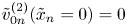 $\tilde {v}_{0n}^{(2)}(\tilde {x}_n=0) =0$ gives a second condition on
 $A(k)$ and
 $B(k)$. Using (3.12), (3.16) and (3.17), we immediately get from (3.10
)
 \begin{equation} A(k)=0, \end{equation}
for  $\epsilon _o k <0$,
 \begin{equation} B(k) = \int_0^{+\infty} \left(\exp({-{\textrm{i}}k \cot(\alpha+ \theta_2)s}) - \exp({-{\textrm{i}}k \cot(\alpha- \theta_2)s}) \right) {\mathcal{F}}(k,s)\,\textrm{d}s, \end{equation}
for  $\epsilon _o k >0$. The functions
 $A(k)$ and
 $B(k)$ are thus fully determined.
As  $\tilde {x} _n \rightarrow +\infty$, expression (3.10) of
 $\tilde {v} _{0n}^{(2)}$ then reduces to
 \begin{equation} \tilde{v}_{0n}^{(2)} \sim \epsilon_o \int _{0}^{+\infty} \exp({{\textrm{i}}k \epsilon_o (\tilde{x}_t + \cot(\alpha +\theta_2) \tilde{x}_n) }) B(\epsilon_o k)\,\textrm{d}k. \end{equation}
Far from the interaction region, the solution is therefore propagating away in the direction  ${\rm \pi} -\theta _2$ (or
 $-\theta _2$ if
 ${\rm \pi} -\theta _2 < \alpha$) and given by (3.13) with
 \begin{equation} G^{(2)}(k) = \varepsilon ^{2} E^{-1/3} \frac{\epsilon_o}{\Lambda^{(2)} }B\left(\frac{k \epsilon_o|\sin(\alpha + \theta_2)|}{\Lambda^{(2)}} \right) \textrm{e}^{k^{3}}, \end{equation}
where  $B(k)$ is defined by (3.17), (3.18), (3.11) and (3.3), assuming
 $x_{\parallel }^{(2)}=1$ at the generation point
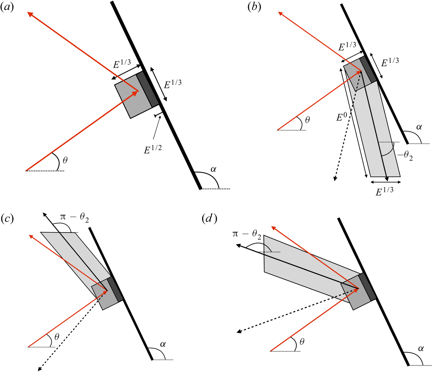
 $I_c$. The different situations are illustrated in figure 3.
Regions where the second-harmonic correction is  $O(\varepsilon ^{2} E^{-1/3})$. Outer region: light grey; interaction region: grey; viscous boundary layer: dark grey. The red arrows indicate the harmonic beam. Here
 $\theta <\alpha <{\rm \pi} -\theta$.
 $(a)$
 $2 \omega > \max (N,2\Omega )$. No second-harmonic beam: the second-harmonic correction is mainly confined in the interaction region and in the viscous boundary layer.
 $(b\text {--}d)$
 $2 \omega < \max (N,2\Omega )$. Second-harmonic beam: the second-harmonic correction extends in an outer region.
 $(b)$
 $N>2\Omega$ and
 $\alpha > {\rm \pi} -\theta _2$. The beam propagates in the direction
 $-\theta _2$.
 $(c)$
 $N>2\Omega$ and
 $\alpha < {\rm \pi} -\theta _2$. The beam propagates in the direction
 ${\rm \pi} -\theta _2$.
 $(d)$
 $N<2\Omega$. The beam propagates in the direction
 ${\rm \pi} -\theta _2$.
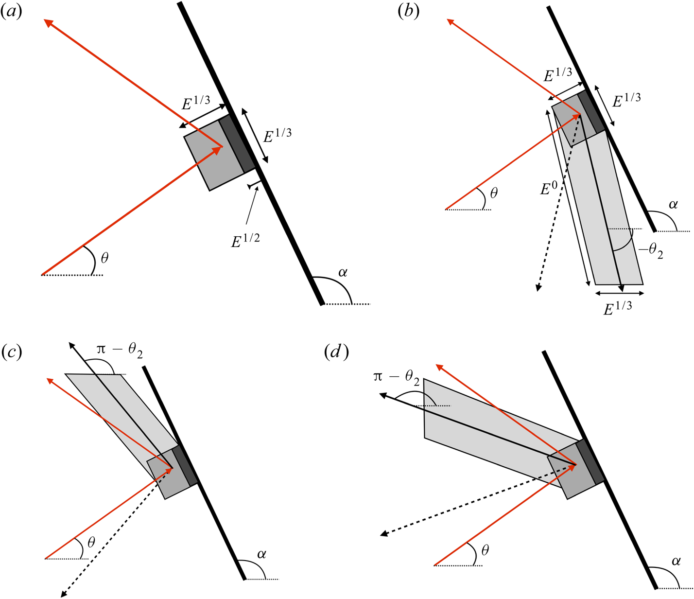
Note that contrarily to the reflected harmonic wave beam, the second-harmonic wave beam does not possess a priori a self-similar structure.
In this section, we have obtained the leading-order expression of the second-harmonic correction in the interaction region and in the beam where it propagates. In the viscous boundary layer where viscous effects become important, the Reynolds stress takes a different form and the no-slip boundary condition has to be applied. As for the harmonic solution, solving this region is needed, if one is interested in finding the first  $O(E^{1/6})$ viscous correction to the solution obtained above.
4. Meanflow correction
The meanflow correction corresponds to a perturbation with a frequency zero. In a stratified and rotating fluid, this frequency is outside the inertia–gravity frequency range, so we do not expect propagation. When  $N$ or
 $\Omega$ vanishes, this is no longer the case: the frequency zero is within the inertia–gravity frequency range. The perturbation propagates horizontally when
 $\Omega =0$ and vertically when
 $N=0$. We therefore expect different situations when
 $N$ or
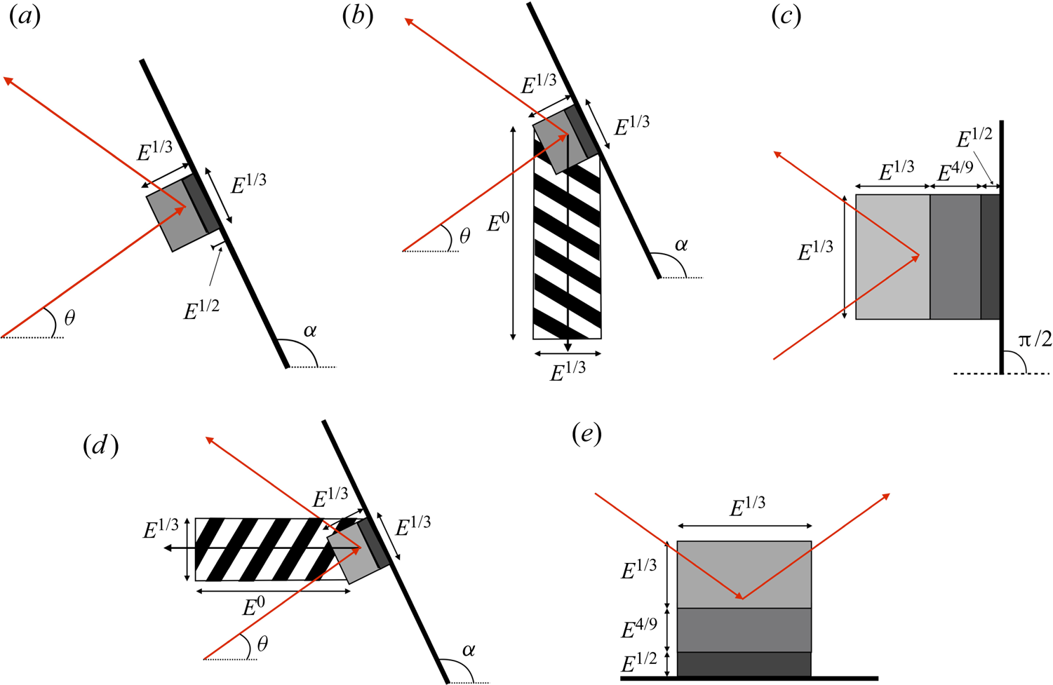
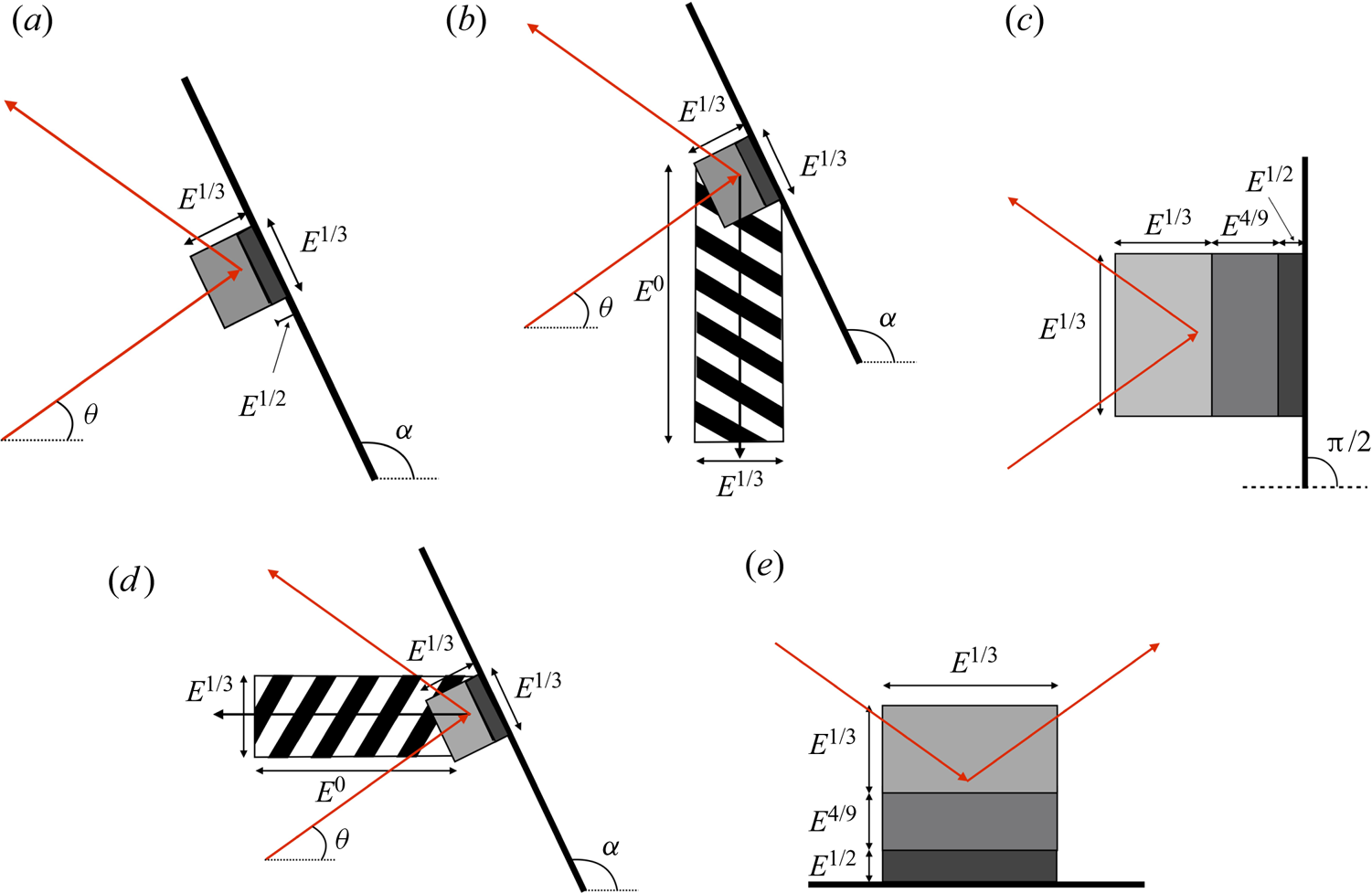
 $\Omega$ vanishes, and when the surface is vertical or horizontal in those cases. What we get is illustrated in figure 4. The goal of the present section is to justify the scaling shown in this figure and provide the structure of the meanflow correction in the different regions for each case.
Regions where the meanflow correction is  $O(\varepsilon ^{2} E^{-1/3})$ (grey regions) or
 $O(\varepsilon ^{2} E^{-1/6})$ (hatched regions). The different levels of grey are associated with different regions (from light to dark: interaction region,
 $E^{4/9}$ viscous layer and viscous boundary layer).
 $(a)$
 $\Omega \neq 0$,
 $N\neq 0$;
 $(b)$
 $\Omega \neq 0$,
 $N=0$,
 $\alpha \neq {\rm \pi} /2$;
 $(c)$
 $\Omega \neq 0$,
 $N=0$,
 $\alpha = {\rm \pi} /2$;
 $(d)$
 $\Omega =0$,
 $N\neq 0$,
 $\alpha \neq 0$;
 $(e)$
 $\Omega =0$,
 $N\neq 0$,
 $\alpha = 0$.
4.1. Generic configuration: rotating and stratified fluid ($N\neq 0$, $\Omega \neq 0$)


In this section, we consider the generic configuration where neither  $N$ nor
 $\Omega$ vanishes. The main contribution is obtained in the interaction region. In this region, the meanflow correction is found to be given by the following ansatz:
 \begin{gather} v_r^{(0)} = \varepsilon^{2} E^{-1/3} \left( \tilde{v}_{0r}^{(0)} \left(\tilde{r},\tilde{z}\right) + E^{1/6} \tilde{v}_{1r}^{(0)} \left(\tilde{r},\tilde{z}\right) + E^{1/3} \tilde{v}_{2r}^{(0)} \left(\tilde{r},\tilde{z}\right)\right) , \end{gather}
 \begin{gather} v_\phi^{(0)} = \varepsilon^{2} E^{-1/3} \left(\tilde{v}_{0\phi}^{(0)} \left(\tilde{r},\tilde{z}\right) + E^{1/6} \tilde{v}_{1\phi}^{(0)} \left(\tilde{r},\tilde{z}\right) + E^{1/3} \tilde{v}_{2\phi}^{(0)} \left(\tilde{r},\tilde{z}\right)\right) , \end{gather}
 \begin{gather} v_z^{(0)} = \varepsilon^{2} E^{-1/3} \left(\tilde{v}_{0z}^{(0)} \left(\tilde{r},\tilde{z}\right) + E^{1/6} \tilde{v}_{1z}^{(0)} \left(\tilde{r},\tilde{z}\right) + E^{1/3} \tilde{v}_{2z}^{(0)} \left(\tilde{r},\tilde{z}\right)\right) , \end{gather}
 \begin{gather} b^{(0)} = \varepsilon^{2} E^{-1/3} \left(\tilde{b}_0^{(0)} \left(\tilde{r},\tilde{z}\right) + E^{1/6} \tilde{b}_{1}^{(0)} \left(\tilde{r},\tilde{z}\right) + E^{1/3} \tilde{b}_{2}^{(0)} \left(\tilde{r},\tilde{z}\right)\right), \end{gather}
 \begin{gather} p^{(0)} = \varepsilon^{2} \tilde{p}_0^{(0)} (\tilde{r},\tilde{z}) , \end{gather}
where  $\tilde {r}$ and
 $\tilde {z}$ are the local variables. Inserting (4.1) in (2.1) using expression (B 2) for the Reynolds stress, the meanflow amplitudes are found to satisfy the equations
 \begin{gather} -2 \Omega \tilde{v}_{0\phi}^{(0)} + \displaystyle\frac{\partial {\tilde{p}_0^{(0)}}}{\partial {\tilde{r}}} = -\tilde{{\mathcal{N}}}_{0r}^{(0)} , \end{gather}
 \begin{gather} 2 \Omega \tilde{v}_{0r}^{(0)} = -\tilde{{\mathcal{N}}}_{0\phi}^{(0)} , \end{gather}
 \begin{gather} \tilde{b}_0^{(0)} + \displaystyle\frac{\partial {\tilde{p}_0^{(0)}}}{\partial {\tilde{z}}} = -\tilde{{\mathcal{N}}}_{0z}^{(0)}, \end{gather}
 \begin{gather} -N^{2} \tilde{v}_{0z}^{(0)} = -\tilde{{\mathcal{N}}}_{0b}^{(0)} , \end{gather}
 \begin{gather} \displaystyle\frac{\partial {\tilde{v}_{0r}^{(0)}}}{\partial {\tilde{r}}} + \displaystyle\frac{\partial {\tilde{v}_{0z}^{(0)}}}{\partial {\tilde{z}}} =0. \end{gather}
Equations (4.2b) and (4.2d) readily give  $\tilde {v}_{0r}^{(0)}$ and
 $\tilde {v}_{0z}^{(0)}$. These expressions are compatible with (4.2e) which is automatically satisfied because of (B 4a). They give normal and tangential velocities as
 \begin{gather} \tilde{v}_{0n}^{(0)} = \sin \alpha \frac{\tilde{{\mathcal{N}}}_{0\phi}^{(0)}}{2\Omega} + \cos\alpha \frac{\tilde{{\mathcal{N}}}_{0b}^{(0)}}{N^{2}} = -2\sin 2\theta \displaystyle\frac{\partial {}}{\partial {\tilde{x}_t}}{\rm Im} \left(\tilde{h}_{\mu}^{(r)} \tilde{h}_{\mu}^{(i)*}\right), \end{gather}
 \begin{gather} \tilde{v}_{0t}^{(0)} = - \cos \alpha \frac{\tilde{{\mathcal{N}}}_{0\phi}^{(0)}}{2\Omega} + \sin\alpha \frac{\tilde{{\mathcal{N}}}_{0b}^{(0)}}{N^{2}} = -2\sin 2\theta \displaystyle\frac{\partial {}}{\partial {\tilde{x}_n}}{\rm Im} \left(\tilde{h}_{\mu}^{(r)} \tilde{h}_{\mu}^{(i)*}\right). \end{gather}
Using (2.19), it is immediately seen that 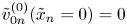 $\tilde {v}_{0n}^{(0)} (\tilde {x}_n =0) = 0$. The condition of non-penetrability is therefore automatically satisfied at leading order. The first-order corrections
 $\tilde {v}_{1r}^{(0)}$ and
 $\tilde {v}_{1z}^{(0)}$ are also directly obtained from the governing equations at the next order:
 \begin{equation} 2\Omega \tilde{v}_{1r}^{(0)} = -\tilde{{\mathcal{N}}}_{1\phi}^{(0)} ,\quad -N^{2} \tilde{v}_{1z}^{(0)}= -\tilde{{\mathcal{N}}}_{1b}^{(0)} , \end{equation}
which gives
 \begin{gather} \tilde{v}_{1n} ^{(0)} = -2 \sin 2\theta \displaystyle\frac{\partial {}}{\partial {\tilde{x}_t}}{\rm Im} \left(C_{1n}^{\infty}\tilde{h}_{\mu +1}^{(r)} \tilde{h}_{\mu}^{(i)*}\right) , \end{gather}
 \begin{gather} \tilde{v}_{1t} ^{(0)} = -2 \sin 2\theta \displaystyle\frac{\partial {}}{\partial {\tilde{x}_n}}{\rm Im} \left(C_{1n}^{\infty}\tilde{h}_{\mu +1}^{(r)} \tilde{h}_{\mu}^{(i)*}\right). \end{gather}
In contrast to  $\tilde {v}_{0n}^{(0)}$,
 $\tilde {v}_{1n}^{(0)}$ does not cancel as
 $\tilde {x}_n\rightarrow 0$.
Equations (4.2a) and (4.2c) are not sufficient to determine the three other amplitudes  $\tilde {v}_{0\phi }^{(0)}$,
 $\tilde {b}_0^{(0)}$ and
 $\tilde {p}_0^{(0)}$. For this purpose, one should consider the governing equations at the third order:
 \begin{gather} 2 \Omega \tilde{v}_{2r}^{(0)} - \bar{{\nabla}}^{2} \tilde{v}_{0\phi}^{(0)} = -\tilde{{\mathcal{N}}}_{2\phi}^{(0)} , \end{gather}
 \begin{gather} -N^{2} \tilde{v}_{2z}^{(0)} - \frac{1}{{Pr}}\bar{{\nabla}}^{2} \tilde{b}_0^{(0)} = -\tilde{{\mathcal{N}}}_{2b}^{(0)} , \end{gather}
 \begin{gather} \displaystyle\frac{\partial {\tilde{v}_{2r}^{(0)}}}{\partial {\tilde{r}}} + \displaystyle\frac{\partial {\tilde{v}_{2z}^{(0)}}}{\partial {\tilde{z}}} + \frac{\tilde{v}_{0r}^{(0)}}{r_c} =0, \end{gather}
where  $\tilde {{\mathcal {N}}}_{2\phi }^{(0)}$ and
 $\tilde {{\mathcal {N}}}_{2b}^{(0)}$ are second-order corrections to the steady Reynolds stress. This system gives the missing equation by plugging the expressions of
 $\tilde {v}_{2r}^{(0)}$ and
 $\tilde {v}_{2z}^{(0)}$ obtained from the first two equations into the third one. If we then replace
 $\tilde {v}_{0\phi }^{(0)}$ and
 $\tilde {b}_0^{(0)}$ by their expression in terms of
 $\tilde {p}_0^{(0)}$ using (4.2a) and (4.2c), we obtain a non-homogeneous fourth-order equation for
 $\tilde {p}_0^{(0)}$ of the form
 \begin{equation} \left(\frac{1}{4\Omega^{2}} \displaystyle\frac{\partial ^{2}{}}{\partial {\tilde{r}}^{2}} + \frac{1}{N^{2} {Pr}} \displaystyle\frac{\partial ^{2}{}}{\partial {\tilde{z}}^{2}} \right) \left( \displaystyle\frac{\partial ^{2}{}}{\partial {\tilde{r}}^{2}} + \displaystyle\frac{\partial ^{2}{}}{\partial {\tilde{z}}^{2}} \right) \tilde{p}_0 ^{(0)} = \tilde{{\mathcal{M}}}(\tilde{r},\tilde{z}). \end{equation}
The function  $\tilde {{\mathcal {M}}}$ can be expressed in terms of the components of
 $\boldsymbol {\tilde {{\mathcal {N}}}_0^{(0)}}$,
 $\boldsymbol {\tilde {{\mathcal {N}}}_1^{(0)}}$ and
 $\boldsymbol {\tilde {{\mathcal {N}}}_2^{(0)}}$. We shall not provide its expression. For the present analysis, it is only important to know that
 ${\tilde {{\mathcal {M}}}}$ is a function localized in the interaction region (i.e.
 $|\tilde {{\mathcal {M}}}| \rightarrow 0$ exponentially fast as
 $\tilde {r}^{2}+\tilde {z}^{2}\rightarrow \infty$). Solutions to (4.7) localized in the interaction region therefore exist. The solution is fully determined upon prescribing
 $\partial _{\tilde {r}} \tilde {p}_0^{(0)}$ and
 $\partial _{\tilde {z}} \tilde {p}_0^{(0)}$ at the boundary
 $\tilde {x}_n=0$. As shown in appendix C, this last step can be made by applying a condition of matching with the solution in the viscous boundary layer.
To summarize this section, we have seen that the radial and axial components are directly forced by the azimuthal and buoyancy component of the Reynolds stress which is of order  $\varepsilon ^{2} E^{-1/3}$ in the interaction region. The azimuthal velocity and the buoyancy turn out to be also
 $O(\varepsilon ^{2} E^{-1/3})$ but they depend on higher corrections of the Reynolds stress and also on the solution in the viscous boundary layer. Velocity components and buoyancy are all found to be localized in the interaction region. This property is also verified by the first-order meanflow correction. This guarantees that no meanflow correction is generated outside the interaction region (at least up to
 $O(\varepsilon ^{2})$ terms).
As we shall see in the next sections, a different conclusion is reached when either  $N$ or
 $\Omega$ cancels.
4.2. Non-stratified case ($N=0$)

In the non-stratified case, the flow is characterized by its velocity and pressure field only and we have  $\omega =2\Omega \cos \theta$ and
 $L_d^{2}= \nu / (2 \Omega \sin \theta )$. The meanflow correction depends on whether the boundary is vertical or not.
4.2.1. Non-vertical boundary ($\alpha \neq {\rm \pi} /2$)

When  $\alpha \neq {\rm \pi} /2$, in the interaction region, the meanflow correction is still given by an ansatz of the form (4.1) with
 $N=0$. It follows that (4.2) applies. The previous expressions for
 $\tilde {v}_{0r}^{(0)}$ and
 $\tilde {v}_{0z}^{(0)}$ are still solutions of the problem, and are such that
 $\tilde {v}_{0n}^{(0)}$ vanishes on the boundary. However, the pressure
 $\tilde {p}_0^{(0)}$ and the azimuthal velocity
 $\tilde {v}_{0\phi }^{(0)}$ are now directly obtained from (4.2a) and (4.2c) because
 $\tilde {b}^{(0)}=0$. We then obtain from these equations
 \begin{gather} \tilde{p}_0^{(0)} = -4 \sin^{2}\theta{\rm Re} \left(\tilde{h}_{\mu}^{(r)}\tilde{h}_{\mu}^{(i)*}\right) + F(\tilde{r}) , \end{gather}
 \begin{gather} \tilde{v}_{0\phi}^{(0)} = -\frac{2}{\Omega} \displaystyle\frac{\partial { }}{\partial {\tilde{r}}}{\rm Re} \left(\tilde{h}_{\mu}^{(r)}\tilde{h}_{\mu}^{(i)*}\right) +\frac{1}{2\Omega} \displaystyle\frac{\partial {F}}{\partial {\tilde{r}}} , \end{gather}
where  $F(\tilde {r})$ is an unknown function. The function
 $F$ is obtained by considering the outer region
 $|z-z_c|=O(1), |r-r_c|=O(E^{1/3})$ where a meanflow could a priori be created. In this region, the Reynolds stress is small and we expect the solution to be a homogeneous solution of the governing equations. Such a solution is given by an ansatz of the form
 $(E^{1/3}u^{(0)},v^{(0)},w^{(0)},E^{1/3}p^{(0)})$ and satisfies the homogeneous equations
 \begin{gather} -2\Omega v^{(0)} +\displaystyle\frac{\partial {p^{(0)}}}{\partial {\tilde{r}}} =0 , \end{gather}
 \begin{gather} 2\Omega u^{(0)} - \displaystyle\frac{\partial ^{2}{v^{(0)}}}{\partial {\tilde{r}}^{2}} = 0 , \end{gather}
 \begin{gather} \displaystyle\frac{\partial {p^{(0)}}}{\partial {z}} - \displaystyle\frac{\partial ^{2}{w^{(0)}}}{\partial {\tilde{r}}^{2}} = 0 , \end{gather}
 \begin{gather} \displaystyle\frac{\partial {u^{(0)}}}{\partial {\tilde{r}}} + \displaystyle\frac{\partial {w^{(0)}}}{\partial {z}} =0. \end{gather}
This system leads to the following equation for  $p^{(0)}$:
 \begin{equation} 4\Omega^{2} \displaystyle\frac{\partial ^{2}{p^{(0)}}}{\partial {z}^{2}} + \frac{\partial^{6} p^{(0)}}{\partial \tilde{r}^{6}} =0. \end{equation}
Using Fourier transform in  $\tilde {r}$, and requiring the solution to vanish far from the boundary, that is as
 $z \rightarrow - \infty$ assuming
 $\alpha >{\rm \pi} /2$, we get for
 $p^{(0)}$
 \begin{equation} p^{(0)} = \int_{-\infty}^{\infty} {\mathcal{P}}(k) \exp\left({|k|^{3} (z-z_c)/(2\Omega) }\right) \textrm{e}^{{\textrm{i}}k\tilde{r}} \, \textrm{d}k. \end{equation}
The other components can all be expressed in terms of  ${\mathcal {P}}(k)$:
 \begin{gather} u^{(0)}= \int_{-\infty}^{\infty} {\textrm{i}}k^{3}{\mathcal{P}}(k)/(2\Omega) \exp\left({|k|^{3} (z-z_c)/(2\Omega) }\right) \textrm{e}^{{\textrm{i}}k\tilde{r}} \, \textrm{d}k , \end{gather}
 \begin{gather} v^{(0)} = -\int_{-\infty}^{\infty} {\textrm{i}}k{\mathcal{P}}(k)/(2\Omega) \exp\left({|k|^{3} (z-z_c)/(2\Omega) }\right) \textrm{e}^{{\textrm{i}}k\tilde{r}} \, \textrm{d}k , \end{gather}
 \begin{gather} w^{(0)} = \int_{-\infty}^{\infty} |k| {\mathcal{P}}(k)/(2\Omega) \exp\left({|k|^{3} (z-z_c)/(2\Omega) }\right)\textrm{e}^{{\textrm{i}}k\tilde{r}} \, \textrm{d}k. \end{gather}
As these expressions should match the forced solution in the interaction region, it is immediate that  $F(\tilde {r}) =0$ and that the forced solution does not excite any outer meanflow at the order
 $\varepsilon ^{2} E^{-1/3}$. The meanflow in this region is created at the next order and is such that
 ${\mathcal {P}}(k) = \varepsilon ^{2} E^{-1/6} {\mathcal {P}}_1(k)$. To obtain
 ${\mathcal {P}}_1(k)$, we must consider the solution in the viscous boundary layer and the forced solution in the interaction region at the next order. The viscous boundary layer solution is given in appendix C Equations (C 1a), (C 1b), (C 1c), (C 5), (C 7) and (C 10) together with (C 6) still apply when
 $N=0$. However, these expressions do not fully define the solution. A second equation for the functions
 $a_t$ and
 $b_t$ is missing. Contrarily to the case
 $N\neq 0$, this equation is obtained by the condition of matching of the azimuthal velocity component. In the viscous boundary layer, the azimuthal velocity can be written as
 \begin{align} & \bar{v}_{0\phi}^{(0)} = {\displaystyle \int_0^{\bar{x}_n} \ \int_{+\infty}^{s} \left(2\Omega \cos\alpha \, \bar{u}_t^{(0)}(\tilde{x}_t,x) + \bar{{\mathcal{N}}}_{0\phi}^{(0)}(\tilde{x}_t, x )\right) \,\textrm{d}x\, \textrm{d}s}\nonumber\\ &\qquad + \displaystyle\frac{a_t(1 -\exp\left({ (-1)^{3/4} \lambda \bar{x}_n})\right) }{ {\textrm{i}} \lambda^{2}} -\displaystyle\frac{b_t(1 -\exp\left({ (-1)^{5/4} \lambda \bar{x}_n}) \right) }{ {\textrm{i}} \lambda^{2}}. \end{align}
In the interaction region, this component is given by (4.1b) and (4.8b) with  $F=0$. The condition of matching then reads
 \begin{align} -\frac{2}{\Omega} \displaystyle\frac{\partial {}}{\partial {\tilde{r}}} \mathrm{Re}\left(\tilde{h}_{\mu}^{(r)}\tilde{h}_{\mu}^{(i)*}\right)\bigg|_{_{\tilde{x}_n=0}} = {\displaystyle \int_0^{+\infty} \ \int_{+\infty}^{s} \left(2\Omega \cos\alpha \, \bar{u}_t^{(0)} + \bar{{\mathcal{N}}}_{0\phi}^{(0)}\right)\,\textrm{d}x \,\textrm{d}s } -\frac{{\textrm{i}}}{\lambda^{2}}(a_t- b_t). \end{align}
This is the second equation that fully determines the solution in the viscous boundary layer. The weak meanflow that is created in the outer region is obtained by matching the normal velocity. The two first orders of the solution in the interaction region are needed to perform such a matching. By collecting the forced solution at the first and second order given by (4.3a) and (4.5a), respectively, and an  $O(\varepsilon ^{2} E^{-1/6})$ homogeneous solution of the form (4.12) that gives a normal velocity component in the outer region
 \begin{equation} v_n^{(0)} = \varepsilon^{2} E^{-1/6} \frac{\cos\alpha}{2\Omega} \int_{-\infty}^{+\infty} |k| {\mathcal{P}}_1(k)\exp\left({|k|^{3} (z-z_c)/(2\Omega) }\right)\textrm{e}^{{\textrm{i}}k\tilde{r}} \, \textrm{d}k , \end{equation}
we obtain, by matching normal velocities, the condition
 \begin{equation} - \int_{0}^{\infty} \partial_{\tilde{x}_t}\bar{u}_t^{(0)}\,\textrm{d}\bar{x}_n + \frac{a'_t -{\textrm{i}}b'_t}{ (-1)^{3/4} \lambda} = \tilde{v}_{1n}^{(0)}|_{_{\tilde{x}_n=0}}+ \frac{\cos\alpha}{2\Omega} \int_{-\infty}^{+\infty} |k| {\mathcal{P}}_1(k)\textrm{e}^{{\textrm{i}}k\tilde{r}} \, \textrm{d}k. \end{equation}
This condition gives the function  ${\mathcal {P}}_1(k)$ that defines the homogeneous solution in the outer region. In the outer region, we therefore expect an axial velocity and an azimuthal velocity of order
 $\varepsilon ^{2}E^{-1/6}$. The different regions for this case are summarized in figure 4
 $(b)$.
4.2.2. Vertical boundary ($\alpha ={\rm \pi} /2$)

This case requires a special treatment because vertical boundaries correspond to critical boundaries for meanflow corrections in a non-stratified fluid. In the interaction region, the forced solution is unchanged and is still given by (4.1a)–(4.1d) with  $N=0$ and
 \begin{gather} \tilde{v}_{0r}^{(0)} = 2\sin 2\theta \displaystyle\frac{\partial {}}{\partial {\tilde{z}}}{\rm Im} \left(\tilde{h}_{\mu}^{(r)} \tilde{h}_{\mu}^{(i)*}\right) , \end{gather}
 \begin{gather} \tilde{v}_{0\phi}^{(0)} = -\frac{2}{\Omega} \displaystyle\frac{\partial { }}{\partial {\tilde{r}}}{\rm Re} \left(\tilde{h}_{\mu}^{(r)}\tilde{h}_{\mu}^{(i)*}\right) , \end{gather}
 \begin{gather} \tilde{v}_{0z}^{(0)} = 2\sin 2\theta \displaystyle\frac{\partial {}}{\partial {\tilde{r}}}{\rm Im} \left(\tilde{h}_{\mu}^{(r)} \tilde{h}_{\mu}^{(i)*}\right) , \end{gather}
 \begin{gather} \tilde{p}_0^{(0)} = -4 \sin^{2}\theta{\rm Re} \left(\tilde{h}_{\mu}^{(r)}\tilde{h}_{\mu}^{(i)*}\right). \end{gather}
The difference appears at higher order and close to the boundary owing to a change of nature of the viscous boundary layer solution (e.g.  $\lambda =0$ in (C 5) when
 $\alpha ={\rm \pi} /2$). A larger viscous layer of width
 $O(E^{4/9})$ appears close to the boundary. To find the solution in this layer, we introduce the new boundary layer variable
 $\check {r}= (r-r_c)/E^{4/9}$ and the ansatz
 \begin{gather} v_r^{(0)} = \varepsilon^{2} E^{-2/9} \left(\partial_{\tilde{r}}\tilde{v}_{0r}^{(0)}|_{_{\tilde{r}=0}} \,\check{r} + \check{v}_{0r}^{(0)} (\check{r},\tilde{z}) \right), \end{gather}
 \begin{gather} v_\phi^{(0)} = \varepsilon^{2} E^{-1/3} \left( \tilde{v}_{0\phi}^{(0)}|_{_{\tilde{r}=0}} \,, + \check{v}_{0\phi}^{(0)} (\check{r},\tilde{z}) \right) , \end{gather}
 \begin{gather} v_z^{(0)} = \varepsilon^{2} E^{-1/3} \left(\tilde{v}_{0z}^{(0)}|_{_{\tilde{r}=0}} \,,+ \check{v}_{0z}^{(0)} (\check{r},\tilde{z}) \right) , \end{gather}
 \begin{gather} p^{(0)} = \varepsilon^{2} \left(\tilde{p}_0^{(0)}|_{_{\tilde{r}=0}} \, + E^{1/9}( \partial_{\tilde{r}}\tilde{p}_0^{(0)}|_{_{\tilde{r}=0}} \, \check{r} + \check{p}_1^{(0)}(\check{r},\tilde{z}) \right), \end{gather}
where the functions  $\check {v}_{0r}^{(0)}$,
 $\check {v}_{0\phi }^{(0)}$,
 $\check {v}_{0z}^{(0)}$ and
 $\check {p}_{1}^{(0)}$ vanish as
 $\check {r} \rightarrow -\infty$ such that the matching with the interaction region is guaranteed. We obtain the system
 \begin{gather} -2 \Omega \check{v}_{0\phi}^{(0)} + \displaystyle\frac{\partial {\check{p}_{1}^{(0)}}}{\partial {\check{r}}} =0 , \end{gather}
 \begin{gather} 2 \Omega \check{v}_{0r}^{(0)} - \displaystyle\frac{\partial ^{2}{\check{v}_{0\phi}^{(0)}}}{\partial {\check{r}}^{2}} = 0 , \end{gather}
 \begin{gather} \displaystyle\frac{\partial {\check{p}_{1}^{(0)}}}{\partial {\tilde{z}}} - \displaystyle\frac{\partial ^{2}{\check{v}_{0z}^{(0)}}}{\partial {\check{r}}^{2}} = 0 , \end{gather}
 \begin{gather} \displaystyle\frac{\partial {\check{v}_{0r}^{(0)}}}{\partial {\check{r}}} + \displaystyle\frac{\partial {\check{v}_{0z}^{(0)}}}{\partial {\tilde{z}}} =0 , \end{gather}
which gives
 \begin{equation} \frac{\partial^{6} \check{p}_{1}^{(0)} }{\partial \check{r}^{6}} + 4\Omega^{2} \displaystyle\frac{\partial ^{2}{\check{p}_{1}^{(0)}}}{\partial {\tilde{z}}^{2}} = 0. \end{equation}
Note that this equation is similar to (4.10) in the outer region. When  $\alpha ={\rm \pi} /2$, the
 $E^{4/9}$ viscous layer thus plays the same role as the outer region. Here, because the boundary corresponds to
 $\check {r}=0$, it is convenient to integrate this equation using Fourier transform in
 $\tilde {z}$. It leads to
 \begin{equation} \check{p}_{1} ^{(0)} = \int_{-\infty}^{+\infty}\left( a_1(k)\textrm{e}^{-\alpha_1\check{r}} + a_2(k)\textrm{e}^{-\alpha_2\check{r} } + a_3(k)\textrm{e}^{-\alpha_3\check{r}}\right)\textrm{e}^{{\textrm{i}}k \tilde{z} } \,\textrm{d}k , \end{equation}
where  $\alpha _j$,
 $j=1,2,3$, are the three roots of
 $\alpha _j^{6} = 4 \Omega ^{2} k^{2}$ with a negative real part (such that
 $\check {p}_{1}^{(0)}$ does vanish as
 $\check {r} \rightarrow -\infty$). The other components are then given by
 \begin{gather} \check{v}_{0r}^{(0)}= -\int_{-\infty}^{+\infty}\left(\sum_{j=1}^{3} \frac{\alpha_j^{3}a_j(k)}{4\Omega^{2}} \textrm{e}^{-\alpha_j\check{r}}\right) \textrm{e}^{{\textrm{i}}k \tilde{z} } \,\textrm{d}k , \end{gather}
 \begin{gather} \check{v}_{0\phi}^{(0)}= -\int_{-\infty}^{+\infty}\left(\sum_{j=1}^{3} \frac{\alpha_ja_j(k)}{2\Omega} \textrm{e}^{-\alpha_j\check{r}}\right)\textrm{e}^{{\textrm{i}}k \tilde{z} } \,\textrm{d}k , \end{gather}
 \begin{gather} \check{v}_{0z}^{(0)}= \int_{-\infty}^{+\infty}\left(\sum_{j=1}^{3} \frac{{\textrm{i}}k a_j(k)}{ \alpha_j^{2}} \textrm{e}^{-\alpha_j\check{r}}\right)\textrm{e}^{{\textrm{i}}k \tilde{z} } \,\textrm{d}k. \end{gather}
The functions  $a_j$,
 $j=1,2,3$ are obtained by matching this solution with the solution in the viscous boundary layer. In the viscous boundary layer, the solution expands, using
 $\bar {r}= \tilde {r}/E^{1/6} = \check {r}/E^{1/18}$, as
 \begin{gather} v_r^{(0)}= \varepsilon^{2} E^{-1/6} \bar{v}_{0r} ^{(0)}(\bar{r},\tilde{z}) , \end{gather}
 \begin{gather} v_\phi^{(0)}= \varepsilon^{2} E^{-1/3} \bar{v}_{0\phi} ^{(0)}(\bar{r},\tilde{z}) , \end{gather}
 \begin{gather} v_z^{(0)}= \varepsilon^{2} E^{-1/3} \bar{v}_{0z} ^{(0)}(\bar{r},\tilde{z}) , \end{gather}
 \begin{gather} p^{(0)}= \varepsilon^{2} \left(\bar{p}_{0} ^{(0)}(\tilde{z}) + E^{1/6} \bar{p}_{1}^{(0)}(\bar{r},\tilde{z})\right) , \end{gather}
and satisfies
 \begin{gather} -2\Omega \bar{v}_{0\phi}^{(0)} + \displaystyle\frac{\partial {\bar{p}_{1}^{(0)}}}{\partial {\bar{r}}} =0, \end{gather}
 \begin{gather} - \displaystyle\frac{\partial ^{2}{\bar{v}_{0z}^{(0)}}}{\partial {\bar{r}}^{2}} + \displaystyle\frac{\partial {\bar{p}_{0}^{(0)}}}{\partial {\tilde{z}}} = - \tilde{{\mathcal{N}}}_{0z}^{(0)}|_{_{\tilde{r}=0}} - \bar{{\mathcal{N}}}_{0z}^{(0)} , \end{gather}
 \begin{gather} -\displaystyle\frac{\partial ^{2}{\bar{v}_{0\phi}^{(0)}}}{\partial {\bar{r}}^{2}} = -\bar{{\mathcal{N}}}_{0\phi}^{(0)}, \end{gather}
 \begin{gather} \displaystyle\frac{\partial {\bar{v}_{0r}^{(0)}}}{\partial {\bar{r}}} + \displaystyle\frac{\partial {\bar{v}_{0z}^{(0)}}}{\partial {\tilde{z}}} = 0. \end{gather}
It follows, using 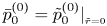 $\bar {p}_0^{(0)} = \tilde {p}_0^{(0)}|_{_{\tilde {r}=0}}$ and the no-slip condition on the boundary, that
 \begin{gather} \bar{v} _{0\phi}^{(0)} = \int_0^{\bar{r}}\!\!\int_{+\infty}^{s} \bar{{\mathcal{N}}}_{0\phi}^{(0)}(x,\tilde{z})\,\textrm{d}x\,\textrm{d}s , \end{gather}
 \begin{gather} \bar{v} _{0z}^{(0)} =\int_0^{\bar{r}}\!\!\int_{+\infty}^{s} \bar{{\mathcal{N}}}_{0z}^{(0)}(x,\tilde{z})\,\textrm{d}x\,\textrm{d}s , \end{gather}
which then gives
 \begin{equation} \bar{v} _{0r}^{(0)} = - \int_0^{\bar{r}} \partial_{\tilde{z}} \bar{v} _{0z}^{(0)}(x,\tilde{z})\,\textrm{d}x. \end{equation}
The matching of the three velocity components between the viscous boundary layer and the  $E^{4/9}$ viscous layer gives
 \begin{gather} -\int_{-\infty}^{+\infty}\left(\sum_{j=1}^{3} \frac{\alpha_j^{3}a_j(k)}{4\Omega^{2}} \right) \textrm{e}^{{\textrm{i}}k \tilde{z} } \,\textrm{d}k =0 , \end{gather}
 \begin{gather} -\int_{-\infty}^{+\infty}\left(\sum_{j=1}^{3} \frac{\alpha_ja_j(k)}{2\Omega} \right) \textrm{e}^{{\textrm{i}}k \tilde{z} } \,\textrm{d}k + \tilde{v}_{0\phi}^{(0)}|_{_{\tilde{r}=0}} = \int_0^{\infty}\ \int_{+\infty}^{s} \bar{{\mathcal{N}}}_{0\phi}^{(0)}(x,\tilde{z})\,\textrm{d}x\,\textrm{d}s , \end{gather}
 \begin{gather} \int_{-\infty}^{+\infty}\left(\sum_{j=1}^{3} \frac{{\textrm{i}}k a_j(k)}{ \alpha_j^{2}} \textrm{e}^{-\alpha_j\check{r}}\right)\textrm{e}^{{\textrm{i}}k \tilde{z} } \,\textrm{d}k + \tilde{v}_{0z}^{(0)}|_{_{\tilde{r}=0}} = \int_0^{\infty}\ \int_{+\infty}^{s} \bar{{\mathcal{N}}}_{0z}^{(0)}(x,\tilde{z})\,\textrm{d}x\,\textrm{d}s. \end{gather}
These three equations permit one to obtain the functions  $a_j$,
 $j=1,2,3$ and therefore the solution in the
 $E^{4/9}$ viscous layer. As the solution in the interaction region, this solution vanishes as
 $|\tilde {z}|\rightarrow \infty$. No solution is therefore created in the outer region for
 $N=0$ when the boundary is vertical. The different regions where the meanflow correction is important are summarized in figure 4
 $(c)$.
4.3. Non-rotating case $(\Omega =0)$

This case is similar to the case  $N=0$, except that critical surfaces for the meanflow correction are now horizontal surfaces. We should then consider the case
 $\alpha =0$ separately. Both cases can be analysed in exactly the same way as for
 $N=0$. The characteristic regions defining the solution for
 $\Omega =0$ are shown in figure 4(d,e).
5. Conclusion
In this work, we have analysed the nonlinear corrections generated by the reflection of a thin axisymmetric beam of frequency  $\omega$ on a solid axisymmetric surface. Although we have focused on self-similar beams emitted by a localized source, the analysis and the scaling remain the same for any other viscous beam of width
 $E^{1/3}$. As also mentioned in § 2, the same analysis can be performed for a thin two-dimensional beam impacting a solid planar surface. In that case, the
 $1/\sqrt {r}$ factor of the similarity solution (2.3) disappears and everything is identical upon replacing
 $r$ by
 $x$ and
 $\phi$ by
 $y$, the only exception being equations (4.6a)–(4.6c) where some curvature terms are present.
As expected, we have shown that a second-harmonic correction and a steady correction are generated in the reflection process. However, both the structure and the scaling of these corrections are different. For the second-harmonic correction, the generation process is purely inviscid. If  $2\omega$ is in the inertial range (that is between
 $2\Omega$ and
 $N$), a strong beam of amplitude
 $\varepsilon ^{2} E^{-1/3}$ is generated. Its structure is similar to the structure obtained by Tabaei etal. (Reference Tabaei, Akylas and Lamb2005) for
 $\Omega =0$. It no longer has the self-similar structure of the harmonic beam but still has a width
 $O(E^{1/3})$ and a persistent length
 $O(1)$. This beam propagates in a particular direction that depends on the inclination angle of the boundary and on whether
 $N$ is larger or smaller than
 $2\Omega$. The different situations are summarized in figure 3.
For the steady correction, the generation process is completely different. In the rotating and stratified case ( $\Omega \neq 0$ and
 $N\neq 0$), the steady correction is as large as the second-harmonic correction (
 $O(\varepsilon ^{2} E^{-1/3}$)) but is confined in the interaction region (
 $O(E^{1/3}$) region around the reflection point). The radial and axial components of the velocity are found to be directly forced by the Reynolds stress by an inviscid mechanism similar to what is known for the non-rotating case (Tabaei etal. Reference Tabaei, Akylas and Lamb2005) while all the other components are generated by a more complex mechanism involving viscous effects.
A steady beam is only observed when either  $\Omega$ or
 $N$ vanishes. In the non-stratified case (
 $N=0$), this beam is a column of width
 $O(E^{1/3})$. In the non-rotating case, it is a horizontal layer of width
 $O(E^{1/3})$. In both cases, the amplitude is
 $O(\varepsilon ^{2} E^{-1/6})$, that is, smaller than the second-harmonic beam but larger than the correction generated in the incident or reflected beam far from the interaction region. These beams are created by the interaction of the incident beam with the viscous correction of the reflected beam. When the boundary is vertical for the non-stratified case, or horizontal for the non-rotating case, the beam is not observed. However, a thickening of the viscous boundary layer to
 $O(E^{4/9})$ is observed close the reflection point. The different configurations for the meanflow correction are summarized in figure 4.
In the present paper, we have considered an axisymmetric beam impacting an axisymmetric surface. It is worth mentioning that a similar analysis can be performed if the beam exhibits a different azimuthal symmetry, for instance an  $m=1$ azimuthal symmetry as in the case of precession or an
 $m=2$ azimuthal symmetry as for a tidal forcing (Le Bars etal. Reference Le Bars, Cébron and Le Gal2015). In those cases, the phase factor associated with the azimuthal symmetry is passive: the second-harmonic correction exhibits a
 $2m$ azimuthal symmetry if the incident beam has an
 $m$ azimuthal symmetry, and the meanflow correction remains axisymmetric. The same conclusion is true for a two-dimensional beam impacting a two-dimensional surface: the beam can exhibit a three-dimensional modulation with an
 $O(1)$ wavenumber without affecting the analysis. In that case, a meanflow correction can indeed be generated during the propagation of the incident beam as shown by Bordes etal. (Reference Bordes, Venaille, Joubaud, Odier and Dauxois2012) and Kataoka & Akylas (Reference Kataoka and Akylas2015) for a purely stratified fluid, but this meanflow correction remains of order
 $\varepsilon ^{2}$ and thus smaller than the one computed here.
As both parameters  $E$ and
 $\varepsilon$ are small, one can naturally address the question of their relative smallness. By performing a weakly nonlinear analysis, we have implicitly assumed that the nonlinear corrections remain small, and smaller than the magnitude of the harmonic solution. This requires
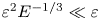 $\varepsilon ^{2} E^{-1/3} \ll \varepsilon$. Actually, the condition of validity of the analysis is stricter. Indeed, the order of the first nonlinear correction oscillating at the frequency
 $\omega$ can be estimated to
 $\varepsilon ^{3}E^{-2/3}$ in the interaction region. For the analysis to be valid, this correction must remain smaller than the first viscous correction of order
 $\varepsilon E^{1/6}$. The condition of validity of the weakly nonlinear analysis is then
 $\varepsilon \ll E^{5/12}$.
6. Comparison with existing results
Only a few studies have focused on thin viscous beams and analysed quantitatively the scaling of the nonlinear corrections generated by the reflection of a wave beam on a solid boundary. The most relevant studies have been performed for rotating flows in the context of planetary applications.
Tilgner (Reference Tilgner2007) computed the meanflow generated by an oscillating tidal mode (azimuthal wavenumber  $m=2$) in a spherical rotating shell (without stratification). In this geometry, the harmonic response depends on the forcing frequency but the wave beam tangent to the inner core at the critical latitude is generally found to be an important feature of the harmonic solution (e.g. Rieutord & Valdettaro Reference Rieutord and Valdettaro2010). For
 $\omega =0.88 \Omega$, Tilgner (Reference Tilgner2007) did observe that the Reynolds stress is mainly localized along this beam, with the largest contributions where the beam interacts with itself, that is, near the points of reflections on the outer boundary, and where beams cross. He computed the meanflow correction but unfortunately used stress-free boundary conditions which makes any comparison with the present results hazardous. Indeed, with stress-free boundary conditions, the solutions in the viscous boundary layers completely change. This affects the viscous correction to the reflected beam, and consequently the meanflow that is generated. Nevertheless, assuming that the normalized harmonic mode is concentrated on a single beam of width
 $E^{1/3}$ and length
 $O(1)$, one can still estimate the two global quantities that Tilgner (Reference Tilgner2007) considered: a characteristic length
 $l = (\int | \boldsymbol {\nabla } \times \boldsymbol {\mathcal {N}}^{(0)}|^{2}\,\textrm {d}V)^{-1/5}$ and the kinetic energy associated with the azimuthal component of the meanflow
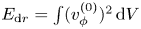 $E_{\textrm {d}r} = \int (v_\phi ^{(0)})^{2}\,\textrm {d}V$ for a harmonic mode of normalized kinetic energy. To get a kinetic energy equal to 1,
 $\varepsilon$ should scale as
 $E^{-1/6}$. It follows from our results that
 $\boldsymbol {\mathcal {N}}^{(0)}$ should scale as
 $\varepsilon ^{2} E^{-2/3}$ in a small domain of volume proportional to
 $E^{2/3}$, which gives
 $l \propto E^{4/15}$, that is, close to but different from the estimate
 $E^{1/3}$ given by Tilgner (Reference Tilgner2007). For the meanflow correction, we expect a scaling in
 $\varepsilon ^{2} E^{-1/6} = E^{-1/2}$, localized in a vertical beam of width
 $E^{1/3}$. This gives
 $E_{\textrm {d}r} \propto E^{-2/3}$. This is clearly different from the proposal in
 $E^{-3/2}$ of Tilgner, but surprisingly not in contradiction with the value
 $E_{\textrm {d}r} \approx 5\times 10^{4}$ obtained for this quantity for
 $\omega =0.88$ at
 $E=10^{-7}$.
More recently, Lin & Noir (Reference Lin and Noir2020) also computed the harmonic flow and the meanflow correction generated by librating a rotating spherical shell. Interestingly, they considered the frequency  $\omega = \sqrt {2} \Omega$ for which the ray trajectories, all inclined at
 $45 ^{\circ }$ with respect to the vertical, form simple patterns. In particular, the ray tangent to the inner core closes on itself after a few reflections on the outer core. Lin & Noir (Reference Lin and Noir2020) did show that the harmonic flow concentrates around this ray with a well-defined structure of width
 $O(E^{1/3})$ and amplitude
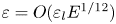 $\varepsilon = O( \varepsilon _l E^{1/12})$, where
 $\varepsilon _l$ is the amplitude of libration. As this scaling corresponds to the prediction obtained by Le Dizès & Le Bars (Reference Le Dizès and Le Bars2017) for the similarity solution generated by a librating sphere in an open domain, one could naturally think that the harmonic solution of Lin & Noir (Reference Lin and Noir2020) may not be far from our beam solution. For the meanflow correction, they did observe vertical localized structures of width scaling as
 $E^{1/3}$ at the location where the beam reflects on the outer boundary, in agreement with the present study. Our scaling for the amplitude would give a meanflow of order
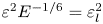 $\varepsilon ^{2}E^{-1/6} = \varepsilon _l^{2}$. Lin & Noir (Reference Lin and Noir2020) observed a weak increase with
 $E$ of the meanflow amplitude that is better fitted by a law in
 $\varepsilon _l^{2} E^{-1/6}$. This may not be in contradiction with our analysis. Indeed, Lin & Noir (Reference Lin and Noir2020) observed this scaling when the beam reflects on a boundary that is librating. In that case, a harmonic flow stronger than the beam is therefore present in the viscous boundary layer that could perhaps explain the enhanced meanflow generation. Unfortunately, they did not document the much weaker meanflow that is generated when only the inner boundary is librating.
Declaration of interests
The author reports no conflict of interest.
Appendix A. Relations between the systems of coordinates
In this work, several coordinate systems are considered in the  $(r,z)$ meridional plane (or equivalently in the
 $(x,z)$ plane):
(i)
${{\boldsymbol {e}}}_\perp ^{(i)}$, ${{\boldsymbol {e}}} _\parallel ^{(i)}$ for the incident beam;(ii)
${{\boldsymbol {e}}}_\perp ^{(r)}$, ${{\boldsymbol {e}}} _\parallel ^{(r)}$ for the reflected beam; and(iii)
${{\boldsymbol {e}}}_t$, ${{\boldsymbol {e}}} _n$ for the boundary.


All can be expressed in terms of the vectors  ${{\boldsymbol {e}}}_r$ and
 ${{\boldsymbol {e}}}_z$ of the cylindrical basis. For the situation illustrated in figure 2
 $(a)$, that is, for
 $0<\theta < \alpha < {\rm \pi} - \theta$, we have the relations
 \begin{gather} {{\boldsymbol{e}}} _\perp^{(i)} = -\sin \theta\, {{\boldsymbol{e}}}_r + \cos \theta\, {{\boldsymbol{e}}}_z , \end{gather}
 \begin{gather} {{\boldsymbol{e}}} _\parallel^{(i)}= \cos \theta\, {{\boldsymbol{e}}}_r + \sin \theta\, {{\boldsymbol{e}}}_z, \end{gather}
 \begin{gather} {{\boldsymbol{e}}} _\perp^{(r)} = \sin \theta\, {{\boldsymbol{e}}}_r + \cos \theta\, {{\boldsymbol{e}}}_z , \end{gather}
 \begin{gather} {{\boldsymbol{e}}} _\parallel^{(r)}= -\cos \theta\, {{\boldsymbol{e}}}_r + \sin \theta\, {{\boldsymbol{e}}}_z, \end{gather}
 \begin{gather} {{\boldsymbol{e}}}_t = \cos \alpha\, {{\boldsymbol{e}}}_r + \sin \alpha\, {{\boldsymbol{e}}}_z , \end{gather}
 \begin{gather} {{\boldsymbol{e}}}_n = \sin \alpha\, {{\boldsymbol{e}}}_r - \cos \alpha\, {{\boldsymbol{e}}}_z. \end{gather}
It also useful to know the relations between the vectors associated with the beam and those associated with the boundary:
 \begin{gather} {{\boldsymbol{e}}} _\perp^{(i)} = \sin (\alpha -\theta)\, {{\boldsymbol{e}}}_t + \cos (\alpha -\theta)\, {{\boldsymbol{e}}}_n , \end{gather}
 \begin{gather} {{\boldsymbol{e}}} _\parallel^{(i)}= \cos (\alpha -\theta)\, {{\boldsymbol{e}}}_t - \sin (\alpha- \theta)\, {{\boldsymbol{e}}}_n, \end{gather}
 \begin{gather} {{\boldsymbol{e}}} _\perp^{(r)} = \sin (\alpha +\theta) \, {{\boldsymbol{e}}}_t + \cos(\alpha+ \theta)\, {{\boldsymbol{e}}}_n , \end{gather}
 \begin{gather} {{\boldsymbol{e}}} _\parallel^{(r)}= -\cos (\alpha + \theta)\, {{\boldsymbol{e}}}_t + \sin (\alpha +\theta)\, {{\boldsymbol{e}}}_n. \end{gather}
Appendix B: Reynolds stress expressions
In the interaction region, the four components of the second-harmonic Reynolds stress can be written as  $\boldsymbol {\mathcal {N}}^{(2)}\sim \varepsilon ^{2} E^{-1/3} \boldsymbol {\tilde {{\mathcal {N}}}_0^{(2)} }$, where
 \begin{equation} \left( \begin{array}{c} \tilde{{\mathcal{N}}}_{0r}^{(2)} \\ \tilde{{\mathcal{N}}}_{0\phi}^{(2)} \\ \tilde{{\mathcal{N}}}_{0z}^{(2)} \\ \tilde{{\mathcal{N}}}_{0b}^{(2)}\end{array} \right) = \left( \begin{array}{c} - 2 \cos^{2}\theta\displaystyle\dfrac{\partial {(\tilde{h}_{\mu}^{(r)} \tilde{h}_{\mu}^{(i)})}}{\partial {\tilde{r}}} \\ -\displaystyle\dfrac{4 {\textrm{i}} \Omega \cos^{2}\theta}{\omega} \displaystyle\dfrac{\partial { (\tilde{h}_{\mu}^{(r)} \tilde{h}_{\mu}^{(i)})}}{\partial {\tilde{r}}} \\ 2\sin^{2}\theta\displaystyle\dfrac{\partial {(\tilde{h}_{\mu}^{(r)} \tilde{h}_{\mu}^{(i)})}}{\partial {\tilde{z}}} \\ - \displaystyle\dfrac{2{\textrm{i}}N^{2} \sin^{2}\theta}{\omega}\displaystyle\dfrac{\partial { (\tilde{h}_{\mu}^{(r)} \tilde{h}_{\mu}^{(i)})}}{\partial {\tilde{z}}} \end{array} \right). \end{equation}
Similarly, the steady Reynolds stress expands (including  $O(E^{1/6})$ corrections) as
 $\boldsymbol {N^{(0)} }= \varepsilon ^{2} E^{-1/3}( \boldsymbol {\tilde {{\mathcal {N}}}_0^{(0)} } + E^{1/6}\boldsymbol {\tilde {{\mathcal {N}}}_1^{(0)} } + \cdots )$, where
 \begin{equation} \left( \begin{array}{@{}c@{}} \tilde{{\mathcal{N}}}_{0r}^{(0)} \\ \tilde{{\mathcal{N}}}_{0\phi}^{(0)} \\ \tilde{{\mathcal{N}}}_{0z}^{(0)} \\ \tilde{{\mathcal{N}}}_{0b}^{(0)} \end{array} \right) = \left( \begin{array}{@{}c@{}} - 4 \cos^{2}\theta \displaystyle\dfrac{\partial {\mathrm{Re} (\tilde{h}_{\mu}^{(r)} \tilde{h}_{\mu}^{(i)*})}}{\partial {\tilde{r}}} \\ -\displaystyle\dfrac{4\Omega\sin 2\theta}{\omega} \displaystyle\dfrac{\partial {\mathrm{Im} (\tilde{h}_{\mu}^{(r)} \tilde{h}_{\mu}^{(i)*})}}{\partial {\tilde{z}}} \\ 4\sin^{2}\theta \displaystyle\dfrac{\partial {\mathrm{Re} (\tilde{h}_{\mu}^{(r)} \tilde{h}_{\mu}^{(i)*})}}{\partial {\tilde{z}}} \\ - \displaystyle\dfrac{2N^{2} \sin 2\theta}{\omega} \displaystyle\dfrac{\partial {\mathrm{Im} (\tilde{h}_{\mu}^{(r)} \tilde{h}_{\mu}^{(i)*})}}{\partial {\tilde{r}}} \end{array} \right) \end{equation}
and
 \begin{equation} \left( \begin{array}{@{}c@{}} \tilde{{\mathcal{N}}}_{1r}^{(0)} \\ \tilde{{\mathcal{N}}}_{1\phi}^{(0)} \\ \tilde{{\mathcal{N}}}_{1z}^{(0)} \\ \tilde{{\mathcal{N}}}_{1b}^{(0)} \end{array} \right) = \left( \begin{array}{@{}c@{}} - 2 \cos^{2}\theta \displaystyle\dfrac{\partial {\mathrm{Re} (C_{1n}^{\infty} \tilde{h}_{\mu +1}^{(r)} \tilde{h}_{\mu}^{(i)*})}}{\partial {\tilde{r}}} \\ -\displaystyle\dfrac{2\Omega\sin 2\theta}{\omega} \displaystyle\dfrac{\partial {\mathrm{Im} (C_{1n}^{\infty}\tilde{h}_{\mu +1}^{(r)} \tilde{h}_{\mu}^{(i)*})}}{\partial {\tilde{z}}} \\ 2\sin^{2}\theta \displaystyle\dfrac{\partial {\mathrm{Re} (C_{1n}^{\infty}\tilde{h}_{\mu +1}^{(r)} \tilde{h}_{\mu}^{(i)*})}}{\partial {\tilde{z}}} \\ - \displaystyle\dfrac{N^{2} \sin 2\theta}{\omega} \displaystyle\dfrac{\partial {\mathrm{Im} (C_{1n}^{\infty}\tilde{h}_{\mu +1}^{(r)} \tilde{h}_{\mu}^{(i)*})}}{\partial {\tilde{r}}} \end{array} \right). \end{equation}
As above, the superscript  $^{*}$ denotes the complex conjugate.
Note in particular that
 \begin{gather} \frac{1}{2\Omega} \displaystyle\frac{\partial {\tilde{{\mathcal{N}}}_{j\phi}^{(0)}}}{\partial {\tilde{r}}} - \frac{1}{N^{2}} \displaystyle\frac{\partial {\tilde{{\mathcal{N}}}_{jb}^{(0)}}}{\partial {\tilde{z}}} =0 , \end{gather}
 \begin{gather} \cos^{2} \theta \displaystyle\frac{\partial {\tilde{{\mathcal{N}}}_{jz}^{(0)}}}{\partial {\tilde{r}}} + \sin^{2} \theta \displaystyle\frac{\partial {\tilde{{\mathcal{N}}}_{jr}^{(0)}}}{\partial {\tilde{z}}} = 0 , \end{gather}
for both  $j=0$ and
 $j=1$.
The Reynolds stress has a different expression in the viscous boundary layer. The expression of the steady Reynolds stress is useful for computing the meanflow correction in § 4. It can be written as
 \begin{equation} \boldsymbol{N^{(0)} }= \varepsilon^{2} E^{-1/3}( \boldsymbol{\tilde{{\mathcal{N}}}_0^{(0)} }|_{_{\tilde{x}_n=0} }+ \boldsymbol{\bar{{\mathcal{N}}}_0^{(0)}}(\tilde{x}_t,\bar{x}_n) + \cdots) , \end{equation}
where
 \begin{equation} \boldsymbol{\bar{{\mathcal{N}}}_0^{(0)}}(\tilde{x}_t,\bar{x}_n) = (\bar{v}_{0t}\partial_{\tilde{x}_t} + \bar{v}_{1n} \partial_{\bar{x}_n} )\left( \begin{array}{@{}c@{}} \bar{v}_{0r} ^{*}\\ \bar{v}_{0\phi}^{*} \\ \bar{v}_{0z} ^{*}\\ \bar{b}_0^{*} \end{array} \right) +\hbox{c.c.}\end{equation}
Appendix C: Meanflow correction in the viscous boundary layer
The viscous boundary layer close to the reflection point extends a distance  $O(E^{1/3})$ along the boundary and a distance
 $O(E^{1/2})$ normal to it. In this appendix, we compute the meanflow correction in this region for a general configuration.
We introduce the boundary layer variable  $\bar {x}_n = (-\sin \alpha (r-r_c) + \cos \alpha (z-z_c))/E^{1/2}$ while keeping the local tangential variable
 $\tilde {x} _t= (\cos \alpha (r-r_c) + \sin \alpha (z-z_c))/E^{1/3}$. The adequate ansatz for the meanflow correction is
 \begin{gather} v_n^{(0)}= \varepsilon^{2} E^{-1/6} \bar{v}_{0n} ^{(0)}(\tilde{x}_t,\bar{x}_n), \end{gather}
 \begin{gather} v_t^{(0)}= \varepsilon^{2} E^{-1/3} \bar{v}_{0t} ^{(0)}(\tilde{x}_t,\bar{x}_n) , \end{gather}
 \begin{gather} v_\phi^{(0)}= \varepsilon^{2} E^{-1/3} \bar{v}_{0\phi} ^{(0)}(\tilde{x}_t,\bar{x}_n) , \end{gather}
 \begin{gather} b^{(0)} = \varepsilon^{2} E^{-1/3} \bar{b}_{0}^{(0)}(\tilde{x}_t,\bar{x}_n) , \end{gather}
 \begin{gather} p^{(0)}= \varepsilon^{2} (\bar{p}_{0} ^{(0)}(\tilde{x}_t) + E^{1/6} \bar{p}_{1}^{(0)}(\tilde{x}_t,\bar{x}_n)). \end{gather}
The governing equations reduce to
 \begin{gather} 2\Omega \sin\alpha \ \bar{v}_{0\phi}^{(0)} - \cos\alpha \,\bar{b}_{0}^{(0)} + \displaystyle\frac{\partial {\bar{p}_{1}^{(0)}}}{\partial {\bar{x}_n}} =0 , \end{gather}
 \begin{gather} -2\Omega \cos\alpha \, \bar{v}_{0\phi}^{(0)} - \sin\alpha \,\bar{b}_{0}^{(0)} - \displaystyle\frac{\partial ^{2}{\bar{v}_{0t}^{(0)}}}{\partial {\bar{x}_n}^{2}} + \displaystyle\frac{\partial {\bar{p}_{0}^{(0)}}}{\partial {\tilde{x}_t}} = - \tilde{{\mathcal{N}}}_{0t}^{(0)}|_{_{\tilde{x}_n=0} }- \bar{{\mathcal{N}}}_{0t}^{(0)} , \end{gather}
 \begin{gather} 2\Omega \cos\alpha \, \bar{v}_{0t}^{(0)} -\displaystyle\frac{\partial ^{2}{\bar{v}_{0\phi}^{(0)}}}{\partial {\bar{x}_n}^{2}} = -\tilde{{\mathcal{N}}}_{0\phi}^{(0)}|_{_{\tilde{x}_n=0} } -\bar{{\mathcal{N}}}_{0\phi}^{(0)} , \end{gather}
 \begin{gather} -N^{2} \sin\alpha \, \bar{v}_{0t}^{(0)} -\frac{1}{{Pr}}\displaystyle\frac{\partial ^{2}{\bar{b}_{0}^{(0)}}}{\partial {\bar{x}_n}^{2}} = -\tilde{{\mathcal{N}}}_{0b}^{(0)}|_{_{\tilde{x}_n=0} } -\bar{{\mathcal{N}}}_{0b}^{(0)} , \end{gather}
 \begin{gather} \displaystyle\frac{\partial {\bar{v}_{0n}^{(0)}}}{\partial {\bar{x}_n}} + \displaystyle\frac{\partial {\bar{v}_{0t}^{(0)}}}{\partial {\tilde{x}_t}} = 0, \end{gather}
where we have used the expressions (B 5) and (B 6) of the Reynolds stress. By definition, the nonlinear terms  $\tilde {{\mathcal {N}}}_{0t}^{(0)}|_{_{\tilde {x}_n=0} }$,
 $\tilde {{\mathcal {N}}}_{0\phi }^{(0)}|_{_{\tilde {x}_n=0} }$ and
 $\tilde {{\mathcal {N}}}_{0b}^{(0)}|_{_{\tilde {x}_n=0} }$ are functions of
 $\tilde {x}_t$ only, obtained from the expressions of the nonlinear terms in the interaction region as
 $\tilde {x}_n\rightarrow 0$, while
 $\bar {{\mathcal {N}}}_{0t}^{(0)}$,
 $\bar {{\mathcal {N}}}_{0\phi }^{(0)}$ and
 $\bar {{\mathcal {N}}}_{0b}^{(0)}$ are functions of
 $\tilde {x}_t$ and
 $\bar {x}_n$ that vanish as
 $\bar {x}_n \rightarrow \infty$.
This system gives for  $\bar {v}_{0t}^{(0)}$
 \begin{equation} \frac{\partial^{4} \bar{v}_{0t}^{(0)}}{\partial \bar{x}_n^{4}} + \left(4\Omega ^{2} \cos^{2}\alpha + N^{2} {Pr} \sin^{2} \alpha^{2}\right) \bar{v}_{0t}^{(0)} = \bar{{\mathcal{Q}}} + \tilde{{\mathcal{Q}}}|_{_{\tilde{x}_n=0} }, \end{equation}
with
 \begin{gather} \tilde{{\mathcal{Q}}}|_{_{\tilde{x}_n=0} } = -2 \Omega \cos\alpha \,\tilde{{\mathcal{N}}}_{0\phi}^{(0)}|_{_{\tilde{x}_n=0} } - {Pr}\sin\alpha \,\tilde{{\mathcal{N}}}_{0b}^{(0)}|_{_{\tilde{x}_n=0} } , \end{gather}
 \begin{gather} \bar{{\mathcal{Q}}} = -2 \Omega \cos\alpha \,\bar{{\mathcal{N}}}_{0\phi}^{(0)} - {Pr}\sin\alpha \,\bar{{\mathcal{N}}}_{0b}^{(0)} + \displaystyle\frac{\partial ^{2}{\bar{{\mathcal{N}}}_{0t}^{(0)}}}{\partial {\bar{x}_n}^{2}}. \end{gather}
A general solution that matches the solution in the interaction region as  $\bar {x} _n \rightarrow \infty$ is obtained in the form
 \begin{equation} \bar{v}_{0t}^{(0)} = \bar{u}_{t\infty} + \bar{u}_t^{(0)} + a_t \exp({ (-1)^{3/4} \lambda \bar{x}_n}) + b_t \exp({(-1)^{5/4} \lambda \bar{x}_n}) , \end{equation}
with  $\lambda = (4\Omega ^{2} \cos ^{2}\alpha + N^{2} {Pr} \sin ^{2} \alpha ^{2})^{1/4}$,
 $\bar {u}_{t\infty }= \tilde {{\mathcal {Q}}}|_{_{\tilde {x}_n=0} }/\lambda ^{4}$, where
 $a_t(\tilde {x}_t)$ and
 $b_t(\tilde {x}_t)$ are arbitrary functions and
 $\bar {u}_t^{(0)}(\tilde {x}_t,\bar {x}_n)$ is a particular solution of (C 3) with only
 $\bar {{\mathcal {Q}}}$ on the right-hand side, which vanishes as
 $\bar {x}_n$ goes to infinity and such that
 $\bar {u}_t^{(0)}(\bar {x}_n=0)=\partial _{\bar {x}_n} \bar {u}_t ^{(0)}(\bar {x}_n=0)=0$. The condition that
 $\bar {v}_{0t}^{(0)}$ vanishes at
 $\bar {x}_n=0$ gives a first condition on
 $a_t$ and
 $b_t$:
 \begin{equation} \bar{u}_{t\infty} + a_t + b_t =0. \end{equation}
The expression of  $\bar {v}_{0n}^{(0)}$ that cancels at
 $\bar {x}_n=0$ is obtained from (C 2e) as
 \begin{align} \bar{v}_{0n}^{(0)} &= -(\partial_{\tilde{x}_t}\bar{u}_{t\infty}) \bar{x}_n -\int_0^{\bar{x}_n} \partial_{\tilde{x}_t}\bar{u}_t^{(0)}(\tilde{x}_t,x)\,\textrm{d}x + \frac{a_t'\left(1 -\exp\left({ (-1)^{3/4} \lambda \bar{x}_n}\right) \right) }{ (-1)^{3/4} \lambda}\nonumber\\ &\quad + \frac{b_t'\left(1- \exp\left({ (-1)^{5/4} \lambda \bar{x}_n}\right)\right)}{ (-1)^{5/4} \lambda}. \end{align}
As  $\bar {x}_n\rightarrow \infty$,
 $\bar {v}_{0t}^{(0)} \sim \bar {u}_{t\infty }$ and
 $\bar {v}_{0n}^{(0)} \sim -(\partial _{\tilde {x}_t}\bar {u}_{t\infty }) \bar {x}_n$. These expressions automatically match the leading-order expressions of
 $\tilde {v}_{0t}^{(0)}$ and
 $\tilde {v}_{0n}^{(0)}$ obtained from (4.3a) and (4.3b) as
 $\tilde {x}_n \rightarrow 0$. To obtain a second condition on
 $a_t$ and
 $b_t$, one then has to consider the next order. This means that we must match the next term in the expansion of
 $\bar {v}_{0n}^{(0)}$ as
 $\bar {x}_n\rightarrow \infty$ with the first-order correction
 $\tilde {v}_{1n}^{(0)}$ of the normal velocity in the interaction region as
 $\tilde {x}_n\rightarrow 0$. This gives
 \begin{equation} - \int_{0}^{\infty} \partial_{\tilde{x}_t}\bar{u}_t^{(0)}\,\textrm{d}\bar{x}_n + \frac{a'_t -{\textrm{i}}b'_t}{ (-1)^{3/4} \lambda} = \tilde{v}_{1n}^{(0)}(\tilde{x}_n=0) , \end{equation}
which can be integrated once in  $\tilde {x}_t$ to give, using (4.5a),
 \begin{equation} - \int_{0}^{\infty} \bar{u}_t^{(0)}\,\textrm{d}\bar{x}_n + \frac{a_t -{\textrm{i}}b_t}{ (-1)^{3/4} \lambda} = -2 \sin 2\theta \mathrm{Im} (C_{1n}^{\infty}\tilde{h}_{\mu +1}^{(r)} \tilde{h}_{\mu}^{(i)*}). \end{equation}
This equation together with (C 6) allows us to get  $a_t$ and
 $b_t$, and therefore
 $\bar {v}_{0t}^{(0)}$ and
 $\bar {v}_{0n}^{(0)}$.
Expressions for  $\bar {v} _\phi ^{(0)}$ and
 $\bar {b}_{0}^{(0)}$ are now deduced from
 $\bar {v}_{0t}^{(0)}$ using (C 2c) and (C 2d):
 \begin{gather} \bar{v} _{0\phi}^{(0)} = \int_0^{\bar{x}_n}\int_{+\infty}^{s} \left(2\Omega \cos\alpha \,\bar{v}_{0t}^{(0)}(\tilde{x}_t,x) + \tilde{{\mathcal{N}}}_{0\phi}^{(0)}|_{_{\tilde{x}_n=0} }(\tilde{x}_t) + \bar{{\mathcal{N}}}_{0\phi}^{(0)}(\tilde{x}_t,x)\right)\,\textrm{d}x \, \textrm{d}s , \end{gather}
 \begin{gather} \bar{b} _0^{(0)} = {Pr} \int_0^{\bar{x}_n}\int_{+\infty}^{s} \left(-N^{2} \sin\alpha \, \bar{v}_{0t}^{(0)}(\tilde{x}_t,x) + \tilde{{\mathcal{N}}}_{0b}^{(0)}|_{_{\tilde{x}_n=0} }(\tilde{x}_t) + \bar{{\mathcal{N}}}_{0b}^{(0)}(\tilde{x}_t,x)\right)\,\textrm{d}x \, \textrm{d}s. \end{gather}
As  $\bar {x}_n \rightarrow \infty$, these expressions must tend to the limits of
 $\tilde {v}_{0\phi }^{(0)}$ and
 $\tilde {b}_0^{(0)}$ as
 $\tilde {x}_n \rightarrow 0$, respectively. Using (4.2a) and (4.2c), they therefore also provide the values of
 $\partial _{\tilde {r}} \tilde {p}_0^{(0)}$ and
 $\partial _{\tilde {z}} \tilde {p}_0^{(0)}$ at
 $\tilde {x}_n=0$.
Note that if  ${Pr} =\infty$ the resolution of the system (C 2) is easier. We immediately get
 $\bar {v}_{0t}^{(0)}$ from (C 2d), then
 $\bar {v}_{0n}^{(0)}$ from (C 2e) with
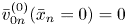 $\bar {v}_{0n}^{(0)}(\bar {x} _n=0)=0$. The function
 $\bar {v} _{0\phi }^{(0)}$ is still given by (C 10a). We then get
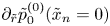 $\partial _{\tilde {r}} \tilde {p}_0^{(0)}(\tilde {x}_n=0)$ from (4.2a) which is the only condition needed to solve (4.7) in that case.