The reunification of German archives has offered historians easier access to the records of the Imperial Statistical Office (Statistisches Reichsamt), which is now housed in Berlin-Lichterfelde (West). Recent historical research in these archives has unearthed important new information from the German industrial census of 1936, which not only permits a reevaluation of German growth in the twentieth century but also makes possible a more careful comparison of British and German industrial productivity in the interwar years. In particular, the new detailed data make it possible to undertake comparisons of real value added at detailed industry levels using the theoretically appropriate double deflation technique.1
“Value added” is sometimes denoted by “net production value,” but we prefer the former term as it is consistent with the terminology in the System of National Accounts. In addition, we use the term deflation for both intertemporal and interspatial comparisons.
See for example Paige and Bombach, Comparison, p. 82. Although the authors advocated the methodology of double deflation, in practice they did not implement it in manufacturing. See also Broadberry, Productivity Race, p. 23. For a long time, double deflation has been the standard procedure for measuring volume changes in value added over time by statistical offices.
Existing international comparisons of productivity in manufacturing for the pre–World War II period relied either on direct quantity comparisons or on single deflation, using relative output prices to convert value added into a common set of prices.3
See Broadberry and Fremdling, “Comparative Productivity”; Broadberry, “Anglo-German Productivity Differences” for United Kingdom-Germany comparisons. Other comparisons will be discussed in what follows.
Reichsamt, Die deutsche Industrie.
Rostas, Comparative Productivity, p. 40.
Our results show that opting for double, rather than single, deflation is not merely the choice of a more sophisticated technique. If firms in different countries were to face similar competitive conditions in both internal and external markets (as firms would, for example, under conditions of a liberal foreign trade regime and a corresponding currency policy), then relative gross output prices might move in tandem with intermediate input prices, as assumed in single deflation. During the 1930s, however, Germany strove for autarky in order to prepare its economy for warfare.6
See the recent detailed studies by Ebi, Export, on foreign trade; and by Höschle, deutsche Textilindustrie, on a specific industrial branch. On the management of the war economy before and during the war see Müller, Manager; and Geer, Markt.
Table 1 presents our major results: it compares labor productivity (real value added per worker) in the United Kingdom and Germany for manufacturing as a whole and for different branches of industry. It is derived using newly calculated relative prices and both for single and double deflation. According to the table Germany had a labor productivity advantage of 5 percent with single deflation and 7 percent with double. Thus on the aggregate level of manufacturing as a whole, both countries had similar labor productivity. Across specific branches of industry, however, there were widespread differences in labor productivity between the two countries. And the magnitude of these differences was sensitive to whether single or double deflation was used.
The choice of single or double deflation did not greatly change the rank order of comparative productivity levels among industrial branches. But Anglo-German differences did become more pronounced in most cases (7 out of 12), with double deflation, and in two instances the comparative performance was even reversed. In particular, German performance in textiles and leather fell much further below British achievements with double deflation. With food manufacturing, however, double deflation raised German labor productivity by taking into account the relatively high German prices of intermediate inputs, such as wheat, brought on by tariffs and the German government's agricultural policy.7
Two recent articles analyzed the severe consequences of high and rising food prices for the standard of living in Germany. Steiner, “Neueinschätzung”; and Baten and Wagner, “Mangelernährung”; see also Abelshauser, “Germany,” pp. 143–47.
An increasing intervention and regulation of the iron and steel branch was put forward by Geer, Markt. For price distortions in 1936 see pp. 39–45.

Although the aggregate results do not depart significantly from previous estimates, the figures for particular industries are strikingly different. If our comparison is used as a new benchmark for time series projection, its effects will be ambiguous. They will depend on how our aggregate results are linked to aggregate indices of manufacturing or on how the estimates for the industrial branches presented here are tied to time series of productivity for each industry.
SOURCES AND DATA
In general, production censuses provide the best data for productivity comparisons. Based on one and the same source, they give information on gross output (quantities and values of products), value added, and employment, which guarantees internal consistency. For the United Kingdom, we took the Census of Production of 1935, which was published by the Business Statistics Office (BSO) of the Board of Trade.9
Board of Trade, Final Report.
In this study, we do not draw on the published version of the German census but on the comprehensive archival records of the German data. We do so for four reasons. First, for military reasons, some branches of industry were hidden by classifying them under misleading headings or by applying a high level of aggregation in the official publication. Second, the archival records give more detailed information on a lower level of aggregation, which makes it easy to fit the German industries into the classifications used in the U.K. census. Third, the published German census provides labor force data only for a single month of the year (usually June), whereas the archival records give the same information for two months (usually June and December). The archival records thus permit precise estimates of labor input and labor productivity. Finally, the archival records provide detailed accounts of the quantities and related values of inputs and outputs for many different manufacturing industries. This allows us to calculate average unit values for a large number of items, which a robust comparison with the UK requires. Because of these characteristics of the unpublished archival records we believe the figures on Germany that we present in this paper are superior to the official census figures published in 1939. Before starting with the comparison of data from this source with the British census of 1935, we will describe the historical background of the German industrial census of 1936, its publication in 1939, and the archival records in some detail.
The German Industrial Census of 1936 and its Publication in 1939
In 1939 the German Imperial Office for Military-Economic Planning (Reichsamt für Wehrwirtschaftliche Planung) published its first and only report on the official Census of Production: Gesamtergebnisse der amtlichen Produktionsstatistik – Die deutsche Industrie.10
Formerly it was the department of industrial statistics of the Imperial Statistical Office (Statistisches Reichsamt). Renamed as Reichsamt für Wehrwirtschaftliche Planung it became an independent institution in 1938. Tooze, Statistics, p. 222.
For a thorough description see Fremdling, “German Industrial Census”; and Fremdling and Stäglin, “Industrieerhebung.”
Surprisingly, the report admits that the industrial census of 1936 was used for planning the war. With this in mind, one wonders why the German Imperial Office published the information at all. Such a publication was not undisputed of course. The central command of the army accused the Imperial Office of having violated secrecy by publishing the report. It demanded that the data be removed from public access.12
Bundesarchiv [hereafter BA] R 3102 / 3082 (letter of 18 August 1939), answers by Leisse 25 August 1939.
BA R 3102 / 3082 F 9. The Imperial Office had planned further publications.
A comparison of the published data of the Imperial Office with the records reveals that the published data seem to be reliable, at least at first glance. For reasons of camouflage, however, certain industries considered important for warfare were hidden by the way the data were aggregated. Basically, the data had been collected for individual plants or industrial units (Betriebsstätten). They then were aggregated by industrial branch. For the sensitive iron and steel industries, for instance, the published statistics covered the entire branch, whereas the archival records distinguished four separate industries. For chemicals, the publication distinguished only seven industries, whereas 38 were noted in the archival records. In addition, certain industries were hidden under misleading aggregates. The foremost example is the aircraft industry. It was supposed to fall under the category of “vehicles” (Fahrzeugindustrie) but it ended up hidden under “construction and others” (Bauindustrie und sonstige Industriezweige). As early as 1936, aircraft industry employed at least 135,210 people.14
BA R 3102 / 5922. In BA R 3102 / 5866 even higher employment data are reported.
These data concern stocks in cotton industry,“Zündererzeugung” (BA R 3102 / 3082 F37, 30.8.1939), “Schusswaffenindustrie,” “Herstellung von Zündstoffen und Sprengkapseln,” and “Sprengstoffindustrie.” See also Sleifer, “Separated Unity”.
Fremdling, “German Industrial Census,” pp. 162–65.
Hoffmann, Wachstum, p. 389.
Comparison of the German and the U.K. Censuses
The starting point for our comparison is the classification of the British Census of Production.18
Board of Trade, Final Report. We did not use the ISIC, to keep as close as possible to the original classification. The British census was the model for the German statisticians. This British viewpoint imputes a British structure to German industry, however, a bias that is unavoidable.
For a detailed documentation see Fremdling, de Jong, and Timmer, “Censuses Compared,” www.ggdc.net.
The area covered by the British census is Great Britain and Northern Ireland. It includes all productive operations in the United Kingdom. For the 1935 census, the Business Statistics Office followed the same procedure as for the census of 1930. Proprietors employing an average of fewer than ten people a year were not required to report detailed returns. Small firms were only asked to give information on the average number of their male and female employees and the nature of the business. Rostas estimated employment not covered by the general reports of the census at 536,600 people, which is about 9.4 percent of total manufacturing employment (small and large firms) in that year.20
Rostas, Comparative Productivity, p. 25.
The German census data comprise the German Empire (Deutsches Reich) within the borders of 1937, thus including Saarland but not Austria and Sudetenland. It basically covered all production units with five employees or more, but in some branches the level of gross output determined what firms were exempt. In several cases, however, all firms were taken into account, for example in mining, fuel, iron and steel, and chemicals.21
In these industries, material inputs were considered to be important for warfare.
Reichsamt, Die deutsche Industrie, pp. 12, 44–55.
Länderrat, Statistisches Handbuch, pp. 238–43.
Rostas maintained that about 500,000 to 600,000 people deliberately were left out in the reported figures of the census (Rostas, “Industrial Production,” p. 42). We did not, however, find such a gap.
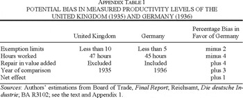
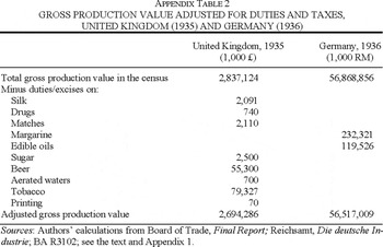
Appendix 1 describes the remaining sources of potential bias between both censuses resulting from differences in hours worked, in year of comparison, and other factors. The net effect on the comparative productivity level was only on the order of one percent (see Appendix Table 1). Because we aim for maximum transparency we did not make any adjustments in our calculations on the aggregate or industry level, except for duties and taxes. For example in the United Kingdom the excise tax on tobacco was paid for by firms on imports into the United Kingdom and not on sales or gross output, as was the case in Germany. To calculate a figure net of the excise, we estimated duties including subtracted drawbacks on tobacco exports from the United Kingdom and then adjusted both intermediate inputs and gross output accordingly (see Appendix Table 2 for details).
NEW RESULTS FROM DOUBLE DEFLATION
Our method of comparing productivity levels is novel in two ways. First, we use producer prices to deflate value added, instead of using the more common quantity approach. Second, we apply double deflation, meaning that we deflate gross output and intermediate inputs separately, rather than doing a single deflation. To understand our approach a brief survey of existing research is necessary. Basically, two main approaches have been used in comparisons of sectoral productivity across nations: the quantity approach and the price approach. Most benchmark estimates before World War II are based on the comparison of physical quantities of output or related methods. These studies focus on output per worker, and follow the methodology of Rostas. In order to aggregate industries or branches of the economy, employment shares or value-added shares are applied.25
Rostas, Comparative Productivity and “Industrial Production.”
The use of the term of “purchasing power parity” in the literature is ambiguous. In the international trade literature, “purchasing power parity” or “PPP” expresses the notion that exchange rates in the world should be such that it is possible to purchase the same bundle of goods and services anywhere in the world with, say, one dollar or one pound. In the work of the International Comparisons Program, the term of “PPP” was diluted and used as a shorthand for the ratio of expenditure prices across countries (Kravis, “Survey”). Ever since, “PPP” has been used as a shorthand for relative prices across countries. We follow this tradition by using the term of “PPP” for any comparison of prices across space, either expenditure, producer output, or input prices.
Kravis, “Survey,” p. 4.
Paige and Bombach, Comparison.
See van Ark, International Comparisons, for an overview of comparisons for the postwar period.
The crucial element in these studies is the estimation of PPPs for output. These are proxied in two ways: by using final expenditure prices and by using unit values based on values and quantities of produced output.30
For comparisons of agricultural output it is sometimes feasible to derive PPPs on the basis of genuine producer output prices, but not for manufacturing, which has a much larger set of goods.
O'Brien and Keyder, Economic Growth, p. 44; Fremdling, “Productivity Comparison,” p. 32; Dormois, “Episodes,” p. 345; see also Broadberry, Productivity Race.
See van Ark and Timmer, “Notes and Communications,” for an elaborate discussion. For ICOP studies for the postwar period, see www.ggdc.net. See de Jong, Catching Up Twice, p. 37, for a prewar comparison of Dutch labor productivity levels with levels in the United Kingdom and Germany using output unit values derived from census data.
Applying the Double Deflation Method
So far, all previous historical studies in the price tradition have relied on a single deflation procedure, deflating value added by a single PPP for gross output. The single deflation method, however, is “not so tidy and conceptually less satisfying.”33
See Paige and Bombach, Comparison, p. 82.
To illustrate this, we provide a very simple example of productivity comparisons based on single and double deflation.34
We thank the editors for this suggestion.
Let us now undertake a labor productivity comparison based on value added (value of output minus value of intermediate input) and single deflation. U.K. value added at U.K. prices is £1 (= £2 – £1) and German value added at German prices is RM20 (= RM60 – RM40) and we need to have a relative price to convert the latter into pounds. With single deflation, we implicitly assume that the output PPP of RM30/£ (= RM60 / £2) is equal to the value added PPP and calculate that real value added in Germany in U.K. prices is £0.67 (= RM20 / RM30 / £). This in turn implies that productivity in Germany is two-thirds the level of productivity in the United Kingdom, which, by construction of the example, is wrong. Double deflation corrects this problem by separately deflating output and intermediate inputs with different PPPs. The intermediate input PPP is higher than the output PPP: RM40 / £ (= RM40 / £1). Thus RM40 intermediate input in Germany deflated by this PPP yields £1. Likewise RM60 of output deflated by relative output prices yields £2, and the real value added in Germany in U.K. prices is £1. This is identical to the U.K. value added, and hence productivity is the same in both countries, which is of course the correct answer. In more complex cases with more inputs (such as capital and other intermediates) and outputs, a similar story holds, but standard index number issues will arise that will yield different answers depending on which country's prices are used as the base in the calculation.
The results in the previous paragraph can also be obtained by deflating the German value added by an appropriate value added PPP. This PPP is the ratio of value added in Germany at U.K. prices (as we calculated in the previous paragraph) to the nominal value added in German prices. Writing the algebra quickly shows that this yields the same results as the direct comparison (see Appendix 2). In the presentation of our results in this article, we proceed by calculating value added PPPs and deflating nominal value added.
There are two main reasons why double deflation has not been applied in practice so far: lack of price data on intermediate inputs and possible volatility of the deflated value added measure. Because value added is the residual between real output and real intermediate input, which have been separately deflated, measurement errors in either set of prices tend to be magnified.35
See Geary, “Concept,” p. 258; and Paige and Bombach, Comparison, p. 81.
Unit values are derived by dividing ex-factory output values by produced quantities for a set of common products in both countries. The unit value can be considered as an average price, averaged throughout the year for all producers and across a group of similar products and sold in domestic as well as foreign markets, thus including exports. Subsequently, in a bilateral comparison, broadly defined products with similar characteristics are matched, for example boilers, cigarettes, margarine, and car tires. For each matched product, the ratio of the unit values in both countries is computed. These product-level unit value ratios need to be aggregated to derive industry-level PPPs. In this aggregation we encounter the familiar index number problems and we deal with them in an appropriate manner (see Appendix 2 for mathematical details). The weights used in aggregation are calculated directly from the British and German census data, both for input and output weights.
PPP Results
We started from estimating the unit value ratios by matching products between the United Kingdom and Germany. Both in the U.K. census and the archival records of the German census, there is a wealth of information on the product level to calculate average prices. For output, it was possible to match 229 products ranging from cotton yarn to various chemical products, for all branches of industry.36
A detailed list of all products and related values/weights can be found in: Fremdling, de Jong, and Timmer, “Censuses Compared,” see www.ggdc.net.

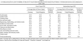
Because we want to employ double deflation, we also matched intermediate inputs. The assumption that the unit value ratio for the matched products is representative of all the unmatched products is harder to make than in the case of outputs, because of the heterogeneity of intermediate inputs. There are, however, many examples of inputs that are recorded for several classes of semi-manufactured products that cover a large fraction of intermediate inputs. This is especially the case in textiles and clothing, with coverage ratios between 46 and 68 percent (see Table 2). In total, 129 matches could be made with a coverage ratio of 35–37 percent for total manufacturing. We were not able to match quantities and values of fuel and electricity because the German census only records the value of the fuel consumption but no related quantities. In many industries, however, the fuel bill is a small fraction of total intermediate input, in most cases less than 5 percent.37
Paige and Bombach, Comparison, p. 193.
Broadberry, Productivity Race, p. 23. He refers to Paige and Bombach and van Ark.
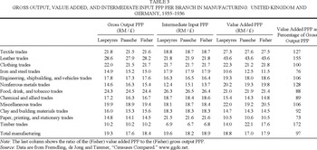
Table 3 provides the gross output, value added, and intermediate input PPPs resulting from the calculations according to the methodology described. We present the Laspeyres, Paasche, and Fisher PPPs that result from our binary comparisons. The ratios differ across industries. Output PPPs are high in the textile, leather, clothing, and food industries. In these industries producer output prices were higher in Germany than in the United Kingdom. In 8 out of the 12 branches the Laspeyres PPP is higher than the Paasche PPP, implying that relative German prices are higher with British weights than with German weights. This is the standard Gerschenkron effect. In a two-country comparison, the Gerschenkron effect implies that the use of quantity weights of one country will lead to an overstatement of the other country's prices, the more the price structures of the two countries differ.39
Gerschenkron, “A Dollar Index.”
See van Ark, Monnikhof, and Timmer, “Prices.”
The studies by Geer (Markt, pp. 40–41); and Höschle (deutsche Textilindustrie, pp. 60–66) present direct evidence of price regulations by the government.

The intermediate input PPPs show a large cross-industry variation too. We find above-average PPPs in leather, clothing, food, and paper. The first three industries also show high output PPPs. In the food industry we find relatively high German input prices for items such as wheat, barley, milk, and unrefined sugar. Germany protected its agricultural sector and therefore relied heavily on relatively expensive home production, whereas Britain imported cereals from overseas. For intermediate inputs, the Laspeyres and Paasche indicators move very close together, the only exception being nonferrous metals. The implication is that individual industries in both countries used similar quantities of intermediate inputs.
Using both output and intermediate input PPPs in equations 8 and 9 of Appendix 2 we now can calculate the double deflated value added PPPs. The results for the value added PPPs are also given in Table 3. Again the difference between Laspeyres and Paasche is small. Using the structure of the branches of manufacturing in Germany or the United Kingdom does not make much difference. The overall Fisher value added PPP is RM17.9 / £. We can compare this figure with alternative estimates. It is, for example, very close to a PPP of RM17.1 / £ calculated by the Institut für Konjunkturforschung for the year 1935.42
This PPP was taken from the Institut für Konjunkturforschung (Institute for Business Cycle Research later named Deutsches Institut für Wirtschaftsforschung DIW). In their Wochenbericht (12, 1939 No. 25) industrial production of the United States and United Kingdom were compared with Germany. It is not clear in which way the converter was calculated precisely. In any case they took an exchange rate of the past, probably the gold exchange rate of 1929 and adjusted it for price movements until 1935, the year of comparison.
Exchange rate from Svennilson, Growth, p. 318.
The last column of Table 3 gives the ratio of the (Fisher) value added PPP to the (Fisher) gross output PPP. This ratio reflects the productivity of capital and labor in the production process. A higher PPP for output than for intermediate input (as with textiles) may indicate that the German textile industry faces higher costs (labor costs, capital costs, or profit margins) than the U.K. industry. The higher costs yield a value added PPP that is larger than the gross output PPP. In 4 out of the 12 branches, the value added PPP is substantially higher than the gross output PPP: textiles, leather, nonferrous metals, and wood products. For iron and steel, and paper and printing, value added PPPs are much lower than gross output PPPs and are even close to the official exchange rate. The cross-industry differences in value added PPP are larger than for gross output. This is to be expected from the double deflation method, where small differences between input and output PPPs tend to be magnified, due to the low share of value added in gross output.
COMPARATIVE VALUE ADDED AND LABOR PRODUCTIVITY BY BRANCH
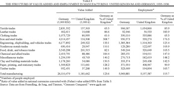
In Table 4, we compare value added and employment by manufacturing branch, using the Fisher value added PPPs to put value added in comparative prices. Total value added of the German census data was 24 percent higher than the U.K. data, and employment about 16 percent.
In both countries the branches of iron and steel, engineering, and nonferrous metals combined comprised the largest sector. The share in Germany made up 42 percent of value added and 41 percent of employment. In the United Kingdom the shares were 33 and 34 percent, respectively. Textiles, leather, and clothing came in second place amounting to 16 percent of value added and 23 percent of employment in Germany versus 21 percent and 32 percent in the United Kingdom. Note that in both countries labor productivity levels were rather low in textiles and just average in the metal industry. On the other hand, both food and chemicals showed high productivity, a sign of great capital intensity. These industries amounted to 23 percent of value added in Germany and employed 14 percent of the labor force, compared to 24.5 and 14 percent, respectively, in the United Kingdom. Output characteristics thus suggest that Germany produced relatively more capital-intensive and intermediate goods (metals, chemicals), while in Britain industries produced consumption goods (textiles, clothing, food, paper and printing).
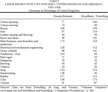
Combining the information on comparative levels of value added in the previous paragraph with our productivity estimates presented in Table 1, we can compare our results with the productivity comparison of Broadberry and Fremdling, who reworked Rostas's comparison based on the physical quantities in the German Statistisches Jahrbuch and the British Census of Production of 1935.44
Rostas, Comparative Productivity.
Broadberry and Fremdling calculated physical output per worker and arrived at an unweighted German average of 101.9 percent of the U.K. level. The ratio rises to 113.7 when employment weights of the United Kingdom are used and remains about the same (102.1) when German weights are applied. The geometric mean of the two weighted ratios can be calculated at 108. In The Productivity Race Broadberry combined these data for certain industrial branches. For aggregation at the industry level he used either German or British employment weights and a geometric mean (in other words the Fisher index). For manufacturing as a whole, however, he opted for an unweighted ratio of 102. Broadberry, Productivity Race, pp. 22–31.

In textiles, leather, and clothing, Broadberry and Fremdling's estimates are higher. We uncovered significant differences for cotton spinning and doubling, because the Germans used low-value waste materials and spun rayon in the production process.46
Höschle, deutsche Textilindustrie, pp. 42–53, 114–28; Müller, Manager, pp. 38–43.
In engineering, shipbuilding, and vehicles our method ranks Germany close to a par with Britain (its index is just above 106, see Table 1). Broadberry and Fremdling give two figures separately for particular industries of this branch (see Table 5): For motor vehicles we found Germany on a par with Britain (its index is just 98) versus the much higher score (141) given by Broadberry and Fremdling. In electrical and mechanical engineering (machinery), however, we calculated 126 compared with 112 by them. Our high score is mainly due to the extraordinary performance of electrical engineering alone where our index reached 155. According to our findings for the entire branch, Britain performed better than has commonly been assumed. Alan Booth recently reached a similar conclusion when he assessed British comparative performance in manufacturing and engineering in particular.47
Booth, “Broadberry-Crafts View,” p. 737.

The food industry reveals the biggest differences between the two studies. Our present estimate for the food industry ranks Germany at 78 percent of the U.K. level (see Table 1). Broadberry and Fremdling calculated a much lower level of 41 percent, being the weighted average of four industries: beet sugar, margarine, brewing, and tobacco. We believe that this gap has to be explained by a number of factors. First, in some industries (notably sugar) we calculated average employment for the entire year, and did not rely on just a seasonal employment peak. Second, there are large differences in coverage. The present estimate includes all food industries (grain milling, cocoa and sugar confectionary, preserved foods, and so on), some of which had somewhat lower levels of productivity in the United Kingdom. Third, we were able to adjust for the relatively high German prices for intermediate inputs, which were brought on by tariffs and Germany's agricultural policy. The result was a less pronounced advantage for the United Kingdom than we would have obtained from physical estimates. Chemical industries show similar patterns. Adjustment for relatively high input prices in Germany resulted in higher levels of value added and thus labor productivity. The clearest example here was seedcrushing, where we got completely reversed productivity levels. In our opinion, the results from double deflation here are far superior to any physical estimation and to single deflation, because differences in relative intermediate input prices mattered a lot in many industries.
CONCLUSIONS
In this study, we presented new estimates of relative productivity performance in manufacturing industries of the United Kingdom and Germany for the years 1935 and 1936 respectively. Using a consistent method, we tried to build a conclusive edifice of comparative Anglo-German levels of value added and labor productivity. This comparison is based on single and double deflation techniques. Four major conclusions can be drawn. First, it seems that on the aggregate level the outcome is unaffected by choice of method. Using single deflation we find that Germany led the United Kingdom in labor productivity by 5 percent, and by 7 percent using our preferred method of double deflation. Both estimates are close to the previous finding of Broadberry and Fremdling, who used a quantity approach and a smaller set of industries.
Second, on the disaggregated level of specific branches, double deflation makes a difference but its advantages are clear. We find a much lower German performance in textiles and engineering branches than Broadberry and Fremdling, but higher levels for nonferrous metal, clay and building materials, iron and steel, and especially food. Our double deflated results seem more plausible because they adjust for big differences in prices of intermediate inputs. The price differences can be tracked back to Germany's striving for autarky, which led to distorted prices and production structures in the 1930s.
Third, our archival evidence invalidates Hoffmann's reconstruction of German national accounts for 1850–1959, which relies on the misleading and incomplete information in the published version of the census. As a result Angus Maddison's data will be affected too because the Hoffmann time series underlie his country entries for Germany.48
Maddison, World Economy.
Albrecht Ritschl recently corrected the Hoffmann-index on German industrial output for the period 1913–1938 by imputing a new series for metal processing. This adjustment yields figures indicating a less marked growth during the interwar period. If, however, Ritschl's time series is extrapolated backwards from our benchmark 1935/36 it yields a very high productivity level for Germany vis-à-vis Britain for the period before World War I, which is far above the benchmark estimates reported by Broadberry and Burhop. A first step in reconciling this contradictory evidence is to produce a completely new time series on industrial output, as suggested by Ritschl. This means making further use of the unpublished 1936-census data and additional archival sources available at the Federal Archive Berlin-Lichterfelde. See the discussion in Ritschl, “Spurious Growth”; Burhop and Wolff, “Compromise Estimate”; and Broadberry and Burhop, “Comparative Productivity.”
Finally, we have shown that the use of double deflation techniques is not only superior in theory, but also feasible in practice. More attempts should be made to apply this method to other sectors and other countries in order to improve benchmark comparisons of productivity performance.
Appendix 1: Comparing the British and German Censuses
Because small companies were treated differently in each country's census, comparative productivity levels for Germany might be biased downwards. The reason is that the German census includes most of the group of firms employing five to ten employees, whereas the British does not. The effect could be large if the level of productivity of small firms was substantially lower than for total manufacturing. Fortunately, the U.K. census gives information on productivity levels by firm size. We calculated that the smallest firms in the British census (between 11 and 24 workers) averaged about 90 percent of the productivity of manufacturing as a whole. We know that the share of the total manufacturing labor force in the firm-group between one to ten workers was about 10 percent in the United Kingdom.50
Rostas, Comparative Productivity, p. 25.

Generally, the concepts of gross output, intermediate input, and value added (or net output) used in both censuses are the same. Net output represents the value added through the manufacturing process, which is the sum of wages, salaries, rent, rates and taxes, depreciation of plant and machinery, advertisement and selling expenses, and profits. This is equal to (gross) census value added at market prices. The only difference is the treatment of repair and maintenance of own capital goods. In the British census, firms had to include the materials used for the repair and maintenance of their own buildings and machinery in the intermediate inputs, whereas in the German statistics they were excluded. From the estimations in the official publication the value of repair and maintenance for total manufacturing can be calculated at RM1,000–1,500 million, which is about 4 percent of total value added.51
Reichsamt, Die deutsche Industrie, pp. 18, 37.
The census years for the comparison between the United Kingdom and Germany differ by one year. Apart from business cycle and capacity utilization effects, we also have to take account of the long-term rise in productivity levels in both economies. To adjust for this we made use of the existing productivity time series estimates and calculated the average movement in productivity levels in both countries between 1935 and 1936.52
See Broadberry, Productivity Race, p. 44.
Finally, an adjustment could be made for differences in hours worked. Ideally, one would measure labor productivity as value added per hour worked, but detailed industry-level estimates of hours worked are not available. According to various sources the average working week in the United Kingdom was 47 hours per week compared to 45 in Germany.53
Rostas, “Industrial Production,” p. 46.
The net effect of these biases on productivity for manufacturing as a whole is summarized in Appendix Table 1.
Adjustments for Duties and Taxes
In general, excise duties and consumer taxes are not included in the value added. For some industries in the census reports, however, duties are included in the gross production value. To put both countries on the same footing, we deducted excises from the gross production value. In the United Kingdom we subtracted excises on silk, drugs, matches, printing, aerated waters, tobacco, sugar, and beer, according to the values mentioned in the General Report of the census. A special case here is the duty on tobacco, which was not paid for by firms on sales or gross output but on imports into the United Kingdom. We estimated this duty, including subtracted drawbacks on tobacco exports from the United Kingdom, at £79,327,000 and adjusted both intermediate inputs and gross output by this number. A similar duty was charged in the petroleum industry but we could not calculate the total amount because firms had been requested to include this in their statement of the cost of materials. In total, we deducted £142,780,000 from the U.K. gross production value. Therefore the gross production value in our study is £2,694.3 million instead of £2,837.1 million in the census. In the case of Britain, this adjustment had no effect on the net production value whatsoever. In the case of Germany, however, the gross production value as well as the value added derived from the archival sources included taxes for certain industries, namely for margarine and edible oils. The figures were adjusted by RM351.8 million.

Appendix 2: Double Deflation
As a first step, unit values (uv) are derived by dividing ex-factory output values (o) by produced quantities (q) for each product i in each country

The unit value can be considered as an average price, averaged throughout the year for all producers and across a group of similar products, sold in domestic as well as foreign markets, thus including exports. Subsequently, in a bilateral comparison, broadly defined products with similar characteristics are matched, for example boilers, cigarettes, margarine, and car tires. For each matched product, the ratio of the unit values in both countries is taken. This unit value ratio (UVR) is given by

A and B are the countries being compared, with A taken as the base country. The product UVR indicates the relative producer price of the matched product in the two countries. Product UVRs need to be aggregated to derive converters for gross output for individual industries or for the aggregate sector. (Henceforth we shall label these converters GO-PPP with a superscript for the country and subscript if a particular industry is concerned.) This can be done in a single step from product to aggregate manufacturing, but also in multiple steps. Because only a selected number of products are matched, the UVRs are then weighted several times, first according to their output share in the individual industry, then according to the industry's share in the branch of manufacturing and finally according to the branch share in manufacturing as a whole. As a result, the aggregate GO-PPP better reflects the actual share of each underlying product item for which UVRs are available in total output. The GO-PPP for industry j based on the industry-of-origin approach is given by

with i =1, . ., Ij,GO the matched output products in industry j; wij = oij / oj the output share of the ith commodity in industry j; and

the total matched value of output in industry j. In bilateral comparisons the weights of either the base country (A) or the other country (B) can be used, which provide a Laspeyres and a Paasche type PPP respectively. The Laspeyres gross output PPP,

, is given by

And the Paasche by

with

the output weights of product i in base country prices and quantities, and

the quantity weights of the other country valued at base country prices. The geometric average of the Laspeyres and Paasche indices, the Fisher index, is often used when a single currency conversion factor is required. PPPs for intermediate input can be derived in a similar way. The Laspeyres intermediate input PPP,

, is given by

And the Paasche by

with i = 1, . ., Ij,II the matched intermediate inputs in industry j with

the intermediate input weights of product i in base country prices and quantities, and

the quantity weights of the other country valued at base country prices. Both the output and the input weights are calculated directly from the census data.
From both output and intermediate input PPPs we can now calculate the double deflated PPPs. Let

and

denote respectively the value of gross output and intermediate input of industry j in country A at national prices, and similarly for B. The Laspeyres value added PPP,

, is then given by

And the Paasche value added PPP,

, is given by

It can easily be seen that in the case of identical gross output and intermediate input PPPs, the value added PPP is the same as the gross output PPP. But if not, the difference between the two depends on the share of intermediate inputs in gross output and the difference between the GO- and II-PPPs.
Fremdling's research was supported by grants from the Netherlands Organisation for Scientific Research (NWO), Deutsches Institut für Wirtschaftsforschung (DIW), and Wissenschaftszentrum Berlin (WZB).