1 INTRODUCTION
A Markov-switching (MS) state-space model extends the linear Gaussian state-space model (henceforth state-space model) by including a latent Markovian discrete regime such that the parameters depend on the regime. Its flexibility to encompass both the continuous and discrete latent variables attracts attention from two strands of literature. First, there is a growing literature on how households form expectations about possible future policy regime changes and how the belief affects the equilibrium (e.g., Schorfheide, Reference Schorfheide2005; Davig and Leeper, Reference Davig and Leeper2011; Bianchi, Reference Bianchi2012, Reference Bianchi2013; Bianchi and Melosi, Reference Bianchi and Melosi2014, Reference Bianchi and Melosi2016, Reference Bianchi and Melosi2017; Bianchi and Ilut, Reference Bianchi and Ilut2017; Song, Reference Song2017). The MS state-space model, as a form of solution to the forward-looking MS rational expectations models (Foerster et al., Reference Foerster, Rubio-Ramírez, Waggoner and Zha2016), is a step toward bringing the model to the data. Second, the MS state-space model has been applied to capture the comovements among macroeconomic variables and asymmetries of business cycle expansions and contractions (e.g., Kim and Yoo, Reference Kim and Yoo1995; Chauvet, Reference Chauvet1998; Kim and Nelson, Reference Kim and Nelson1998; Diebold and Rudebusch, Reference Diebold and Rudebusch1999).
Apart from providing flexibility, inclusion of the latent regime into the state-space model also brings challenges to maximum likelihood estimation. The problem of path dependence arises during the application of the Kalman filter. For state-space models, the simple-to-implement Kalman filter can be applied to the likelihood computation, because the conditional distribution of the state given past observations is Gaussian, and its mean and variance coincide with the sequence of linear projections in the Kalman filter. After the inclusion of the regime process, Gaussianity holds only if the distribution is also conditioned on the entire regime path. Any truncation in the path causes the conditional distribution of the state to be a Gaussian mixture instead of Gaussian, and the linear projections fail to provide exact conditional means and variances. As a result, for MS state-space models, the Kalman filter must be computed for each entire regime path. The computation is, however, practically infeasible owing to the curse of dimensionality. Even if there are only two regimes, after 10 periods, the number of regime paths grows to over 1,000.
To make the Kalman filter computationally feasible, Kim (Reference Kim1994) formulated an approximation strategy, based on Harrison and Stevens (Reference Harrison and Stevens1976). This strategy tracks only the most recent r periods of the regimes, instead of the entire regime history. To keep the number of regime periods at r, it adds a collapsing step at the end of each Kalman-filter iteration and averages out the most dated regime. We refer to this filter as the Kalman-collapsing filter. The outputs of the Kalman-collapsing filter are then used in place of the mean and variance of the Gaussian function assumed on the predictive density given the r regimes. This is where the approximation enters. The true predictive density given r regimes is a Gaussian mixture, but a Gaussian density is assumed on it. The Kalman-collapsing filter outputs are not the true means and variances but are treated as if they were. This approximation strategy is then widely applied in many empirical works, such as Chauvet (Reference Chauvet1998), Bianchi and Ilut (Reference Bianchi and Ilut2017), Bianchi, Ilut, and Schneider (Reference Bianchi, Ilut and Schneider2018), Chang, Maih, and Tan (Reference Chang, Maih and Tan2021), Davig and Leeper (Reference Davig and Leeper2011), and Schorfheide (Reference Schorfheide2005).
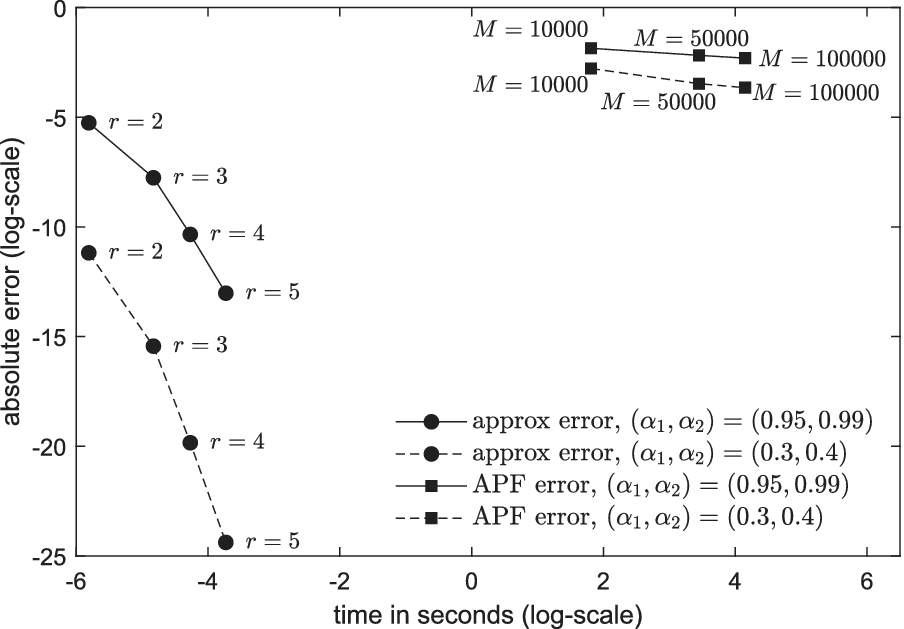
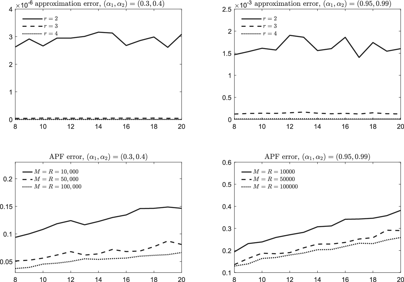
Despite the popularity of the approximation strategy by Kim (Reference Kim1994), its statistical properties have not been analyzed. Kim and Kang (Reference Kim and Kang2019) attempted to use simulation to examine the approximation error. Although their simulation experiments are extensive, they cannot cover all possible setups and parameter values. So far, there are no theoretical studies that quantify the effect of the approximation on likelihood computation and latent variable inference. Thus, many empirical studies resorted to particle filters, as explicitly pointed out in Kim and Nelson (Reference Kim and Nelson1998). The computation of particle filters, though feasible, is still expensive because of the random sampling procedure at each particle and each iteration. Moreover, from the simulation experiments in Section 7.4, the computation error of the auxiliary particle filter could be larger than the error caused by the approxi mation. It would be a loss to simply disregard the approximation strategy, and thus theoretical studies on its reliability are called for. Furthermore, the asymptotic properties of the maximum likelihood estimator (MLE) using the approximation strategy have not been examined. Meanwhile, many empirical studies reported standard errors and test results based on the presumed asymptotic normality (e.g., Kim and Yoo, Reference Kim and Yoo1995; Chauvet, Reference Chauvet1998; Kahn and Rich, Reference Kahn and Rich2007; Morley and Piger, Reference Morley and Piger2012). This study, therefore, provides a theoretical analysis to fill these gaps.
We first derive an upper bound of the approximation error in the likelihood computation. To fix ideas, we briefly introduce the MS state-space model considered in this article:

where
$x_t$
 is a latent state variable,
$y_t$
 is the observed variable, and the parameters depend on a latent regime variable
$s_t$
 . The upper bound includes
$\alpha _{\max }^{r-1}$
 , where
$\alpha _{\max }$
 denotes the maximum absolute value of the regime-specific autoregressive coefficient
$\alpha _{s_t}$
 in the latent state equation. It is derived from two findings. First, from the expressions of the exact and approximate likelihood functions, the approximation error lies in the distance between the Kalman-collapsing filter outputs and the Kalman filter outputs. The Kalman-collapsing filter includes the extra collapsing step, which averages out the regime r periods ahead. Thus, the difference is essentially the discrepancy between the average and each path, which is further bounded by the maximum distance between any two paths different only at the regime r periods ahead. Second, the Kalman filter is convergent. That is, for two iterations different only at their starting points, their difference decays exponentially at rate
$\alpha _{\max }$
 . Together, these two findings result in the upper bound as
$\alpha _{\max }^{r-1}$
 . Thus, the approximation error increases with
$\alpha _{\max }$
 . This state transition coefficient links the previous period to the current period. As it gets closer to zero in all regimes, the influence of past information vanishes faster, and the difference caused by the approximation procedure gets smaller.
We also examine the error in the latent variable inference caused by approximation. In many studies, the latent variables themselves are of economic interest. For instance, Bianchi (Reference Bianchi2013) made inference on the regimes to understand the central bank’s behavior across monetary policy regimes. Chauvet (Reference Chauvet1998) inferred the state to track changes in aggregate economic activity. We focus on three types of inferences of the latent variables at time t, the predictive inference using information up to time
$t-1$
 , the updated inference using information up to time t, and the smoothed inference using the full sample. For all three types of inferences,
$\alpha _{\max }^{r}$
 enters the upper bounds of errors. Moreover, the error in smoothed inference is larger than the error in updated and predictive inference.
In addition, we show consistency and asymptotic normality of the approximate MLE, if r increases with the sample size at appropriate rates, and give consistent estimates of the asymptotic covariance matrix. The proof consists of two steps. First, we show that the normalized likelihood function, score function, and Hessian matrix converge to the exact ones uniformly if r increases with the sample size at permissible rates, provided that
$\alpha _{\max }$
 is smaller than unity uniformly. Second, we show consistency and asymptotic normality of the exact MLE. The asymptotic properties of the MS state-space models fit into the statistical literature of hidden Markov models because the latent state and regime jointly follow a Markov process and, when conditioned on the state and regime, the observation process is independent and identically distributed. Consistency follows from Douc and Moulines (Reference Douc and Moulines2012), which shows consistency in a wide range of hidden Markov models. For asymptotic normality of the MLE, the general difficulty is that the sequence of predictive distributions of the latent process given past observations is not stationary. Thus, the law of large numbers or central limit theorems cannot be applied directly. The strategy, originating from Baum and Petrie (Reference Baum and Petrie1966), is to make an approximation with a stationary sequence. Previous studies established this approximation under two assumptions: first, the transition density of the latent process is bounded away from zero; second, the score function and the Hessian are bounded above uniformly (Bickel, Ritov, and Rydén, Reference Bickel, Ritov and Rydén1998; Jensen and Petersen, Reference Jensen and Petersen1999; Douc, Moulines, and Rydén, Reference Douc, Moulines and Rydén2004; Kasahara and Shimotsu, Reference Kasahara and Shimotsu2019; Pouzo, Psaradakis, and Sola, Reference Pouzo, Psaradakis and Sola2022; Li and Liu, Reference Li and Liu2023). These two assumptions more or less restrict the latent process to take values on a compact space, and thus, they do not hold in MS state-space models. We rely on two instruments to show the asymptotic normality. The first one is the uniform forgetting of the filtering distribution established by Douc and Moulines (Reference Douc and Moulines2012). It imposes a less restrictive assumption on the transition density and only requires a positive lower bound on a large enough set, which holds in MS state-space models. For the second instrument, we show that the score function and Hessian at each period are bounded above by random variables with finite second moments, which suffices to show the approximation in probability.
It is worth mentioning that the theoretical analysis in this study is based on our newly proposed collapsing method, which discards a nonlinear adjustment term in Kim (Reference Kim1994). Our simple collapsing step serves the same function as that of Kim (Reference Kim1994) to average out the most dated regime. Kim (Reference Kim1994) includes the nonlinear adjustment term based on the argument that it would help to yield the exact expressions if the outputs of the Kalman-collapsing filter were exact means and variances. The outputs are, however, approximations instead of the exact means and variances. There is no theoretical support for the nonlinear term in Kim (Reference Kim1994). On the other hand, the simple collapsing step facilitates the theoretical derivation and enables us to focus on the real theoretical challenges. We also show through simulations that the difference caused by discarding the nonlinear terms is small.
The article is organized as follows. Section 2 presents the MS state-space model, clarifies the causes of path dependence, and explains the algorithm to calculate the approximate likelihood function. Section 3 derives explicit expressions of the exact and approximate likelihood functions, analyzes their difference, and builds upper bounds for the approximation errors in likelihood computation and latent variable inference. Section 4 shows consistency and asymptotic normality of the approximate MLE. Section 5 provides practical guidelines for assessing approximation errors and choosing the truncation parameter r. Section 6 discusses the challenges in determining the number of regimes and directions for future research. Section 7 presents simulation experiments. Section 8 concludes the article.
Notation:
$\triangleq $
 denotes “equal by definition.”
$\Rightarrow $
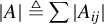
 denotes weak convergence. For a matrix or vector A,
$|A|\triangleq \sum |A_{ij}|$
 .
$\lfloor x\rfloor $
 denotes the largest integer less than or equal to x. Boldface letters denote vectors. For any scalar sequence
${y_t}$
 , let
$\mathbf {y}_m^n\triangleq (y_{m},\ldots ,y_n)'$
 for
$m\leq n$
 , and let
$\mathbf {y}_m^n$
 be empty for
$m>n$
 . The same convention applies to all other variables. For a vector-valued function
$\mathbf {f}(x) = (f_1(x),\ldots ,f_n(x))'$
 ,
$\int \mathbf {f}(x)d\mu (x)\triangleq \big (\int f_1(x) d\mu (x),\ldots ,\int f_n(x) d\mu (x) \big )'$
 .
2 THE MODEL, PATH DEPENDENCE, AND APPROXIMATION
This section describes the MS state-space model, explains the causes of path dependence during the application of the Kalman filter, and explains the approximation algorithm in Kim (Reference Kim1994) and our collapsing method to average out regimes.
2.1 The Model, Assumptions, and Notation
Consider the following MS state-space model:


where the transition equation describes the evolution of a latent variable
$x_t$
 , and the measurement equation describes how the observed variable
$y_t$
 responds to
$x_t$
 . The disturbances,
$v_t$
 and
$u_t$
 , are mutually and serially independent and follow standard normal distributions. The parameters
$\beta _{s_t}$
 ,
$\sigma _{s_t}$
 ,
$\alpha _{s_t}$
 , and
$\varsigma _{s_t}$
 depend on a latent regime variable
$s_t$
 . We assume that
$s_t$
 follows a first-order Markov chain on
$\mathbb {S}=\{1,2,\ldots ,J\}$
 with transition matrix
$(q_{ij})_{1\leq i,j\leq J}$
 and
$q_{iJ}=1-\sum _{j=1}^{J-1}q_{ij}$
 ,
$i=1,2,\ldots ,J$
 . Moreover, we assume
$\sigma _j,\varsigma _j>0$
 for all
$j=1,\ldots ,J$
 . The unknown parameter is
$\theta = \big ( (\beta _i,\sigma _i,\alpha _i,\varsigma _i)_{i\in \mathbb {S}}, (q_{ij})_{1\le i\le J,\,1\le j\le J-1} \big )$
 , and
$\theta _0$
 denotes the true parameter. We write
$\mathbb {E}_\theta $
 ,
$\mathbb {P}_\theta $
 , and
$p_\theta $
 when the parameter is
$\theta $
 , and
$\mathbb {E}_0$
 ,
$\mathbb {P}_0$
 , and
$p_0$
 when the parameter is
$\theta _0$
 .
Assumption 1 (Identification).
For identification, we impose the following normalizing conditions: (i)
$\varsigma _j=1$
 for some j; (ii)
$\beta _j> 0$
 ,
$j=1,\ldots ,J$
 ; (iii)
$\alpha _j\neq 0$
 ,
$j=1,\ldots ,J$
 ; and (iv)
$\beta _i^2\varsigma _i^2+\sigma _i^2\neq \beta _j^2\varsigma _j^2+\sigma _j^2$
 and
$\beta _i\alpha _i\neq \beta _j\alpha _j$
 for
$i\neq j$
 .
Remark 1. In Assumption 1, we impose (i) because for
$c\neq 0$
 , (1) remains invariant under the joint transformation
$x_t\mapsto cx_t$
 ,
$\beta _{s_t}\mapsto \beta _{s_t}/c$
 , and
$\varsigma _{s_t}\mapsto c\varsigma _{s_t}$
 . For (ii), we first impose
$\beta _j\neq 0$
 ,
$j=1,\ldots ,J$
 , for the identification of
$\alpha _{s_t}$
 . If
$\beta _j= 0$
 , then
$y_t=\sigma _j u_t$
 for
$s_t=j$
 . The conditional distribution
$y_t|(s_t=j)$
 is i.i.d.
$\mathbb {N}(0,\sigma _j^2)$
 , regardless of the value of
$\alpha _j$
 . We impose
$\beta _j>0$
 ,
$j=1,2,\ldots ,J,$
 for the identification of
$\beta _j$
 . To see this, note that
$(v_t)$
 has the same distribution as
$(-v_t)$
 . The measurement equation is invariant under the joint transformation
$\beta _{s_t}\mapsto -\beta _{s_t}$
 ,
$x_t\mapsto -x_t$
 , and
$v_t\mapsto -v_t$
 . For (iii), if
$\alpha _j=0$
 , then (1) is invariant under the joint transformation
$\beta _{j}\mapsto c\beta _{j}$
 and
$\varsigma _{j}\mapsto \varsigma _{j}/c$
 for
$c>0$
 . (iv) ensures that different regime sequences
$(s_1,\ldots ,s_n)$
 lead to different variances of the conditional distribution
$p_\theta (y_1,\ldots ,y_n|x_0,s_1,\ldots ,s_n)$
 . This guarantees that distinct regime sequences are distinguishable through the conditional distribution. To avoid the identification problem caused by the permutation of the regimes, we restrict
$\beta _i^2\varsigma _i^2+\sigma _i^2<\beta _j^2\varsigma _j^2+\sigma _j^2$
 for
$i<j$
 .
In the special case of
$J=1$
 , the model reduces to a state-space model. The Kalman filter can be applied to compute the likelihood, because the conditional distribution in (3) is Gaussian,

and the linear projections in the Kalman filter coincide with the mean and variance of (3). When
$J\geq 2$
 , Gaussianity holds only if the distribution is also conditioned on the entire path of the regime. The Kalman filter needs to be applied to all possible regime paths to deliver the likelihood function. Then the problem of path dependence arises, which is explained in detail in Section 2.2.
2.2 Path Dependence in the Application of the Kalman Filter
$\mathbf {y}_1^t$
 and
$x_t$
 can be written as a linear combination of the Gaussian shocks
$\mathbf {u}_1^t$
 and
$\mathbf {v}_1^t$
 with coefficients that depend on the regimes:

By the property of the Gaussian distribution,

If the Kalman filter is applied, it must be computed for each entire regime path
$\mathbf {s}_1^t$
 in order to derive the mean and variance in (4). If we truncate the regime path and only consider the most recent r periods, then the distribution of
$(x_t,y_t)' \mid (\mathbf {y}_1^{t-1},\mathbf {s}_{t-r+1}^t,x_0)$
 becomes a Gaussian mixture, rather than Gaussian. In this case, the outputs of the Kalman filter no longer coincide with the mean and variance of the Gaussian mixture distribution, and the exact distribution cannot be recovered. Hence, to obtain the exact distribution, one must condition on the entire regime path.
Tracking all regime paths is computationally infeasible owing to the curse of dimensionality. More specifically, the Kalman filter given path
$\mathbf {s}_1^t$
 is


$t=1,2,\ldots $
 , where
$x_{t|k}^\theta (\mathbf {s}_1^t)$
 (resp.
$y_{t|k}^\theta (\mathbf {s}_1^t)$
 ) denotes the linear projection of
$x_t$
 (resp.
$y_t$
 ) given the observation history
$\mathbf {y}_1^k$
 and the regime history
$\mathbf {s}_1^t$
 , and
$\Omega _{t|k}^\theta (\mathbf {s}_1^t)$
 (resp.
$\Sigma _{t|k}^\theta (\mathbf {s}_1^t)$
 ) denotes the mean squared error of
$x_t$
 (resp.
$y_t$
 ) given the observation history
$\mathbf {y}_1^k$
 and the regime history
$\mathbf {s}_1^t$
 . Then (5)–(10) need to be computed for all possible regime paths
$\mathbf {s}_1^t$
 , the number of which is
$J^t$
 . Because the number of paths increases geometrically, the computation quickly becomes practically infeasible.
It is worth pointing out that path dependence only arises when the Kalman filter is applied to compute the likelihood. It does not arise if we use simulation-based filters, such as particle filters. For simulation-based filters, the period likelihood
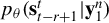
$p_\theta (y_t|\mathbf {y}_1^{t-1})$
 can be sequentially computed from

where
$w_t=(x_t,s_t)'$
 . The integral can be dealt with numerically in the simulation-based filters. At time t, information about previous unobservable variables,
$w_{t-1}$
 , is integrated out in (11), and thus we do not need to keep track of past regimes. The computation of simulation-based filters, though feasible, is still expensive because of the random sampling procedure at each sample and each iteration. In order to reduce computation time and still enjoy the simplicity of the Kalman filter, many empirical works apply an approximation strategy, which is explained in Section 2.3.
2.3 The Approximation Algorithm
This section explains the approximation algorithm in Kim (Reference Kim1994) and our collapsing method to average out the regimes. During the application of the Kalman filter, the approximation algorithm truncates the regime path and tracks only the most recent r periods of regimes,
$\mathbf {s}_{t-r+1}^t$
 , for
$t\geq r$
 . The likelihood function computed with this algorithm is approximate. We use
$\overline {p}_r^\theta $
 to denote the approximate likelihood function, with the subscript r emphasizing that it depends on the regime path length r.
The Kalman filter given the most recent r periods of regimes can be described as in (12)–(17).


We put lines over the variables in (12)–(17) to distinguish them from the ones used in the exact algorithm (5)–(10). After the iteration at time t,
$\overline {x}^\theta _{t|t}(\mathbf {s}_{t-r+1}^t)$
 and
$\overline {\Omega }^\theta _{t|t}(\mathbf {s}_{t-r+1}^t)$
 depend on r periods of regimes. If we directly go to the filter at time
$t+1$
 , then we will include one more regime
$s_{t+1}$
 and track
$r+1$
 regimes. If we keep doing it, the number of regimes increases geometrically. To avoid the increase, we need to average out, or collapse, the most dated regime. Then the number of periods of regimes is
$r-1$
 at the end of iterations at time t and stays at r at time
$t+1$
 . Kim (Reference Kim1994) adopts the following collapsing procedures:


We propose the following new method to collapse
$\overline {\Omega }^\theta _{t|t}(\mathbf {s}_{t-r+2}^{t})$
 by discarding the nonlinear adjustment term in (19):

To see more clearly how the two collapsing rules differ, note that their gap is

which measures the dispersion of
$\overline {x}_{t|t}^\theta (\mathbf {s}_{t-r+1}^t)$
 across different values of
$s_{t-r+1}$
 . The gap is small when
$\max _{i,j\in \mathbb {S}}|\overline {x}_{t|t}^\theta (\mathbf {s}_{t-r+2}^t,s_{t-r+1}=i)-\overline {x}_{t|t}^\theta (\mathbf {s}_{t-r+2}^t,s_{t-r+1}=j)|$
 is small. As shown in the proof of Theorem 11, in the simple collapsing method, this per-period gap is small when
$\max _{j\in \mathbb {S}}\alpha _j$
 is small and r is large. This suggests that the gap between the two collapsing rules may likewise depend on
$\max _{j\in \mathbb {S}}\alpha _j$
 and r. Moreover, because the gap occurs in every period, the cumulative difference over the sample of size n increases with n.
Kim (Reference Kim1994) includes the nonlinear term based on the argument that if
$\overline {x}^\theta _{t|t}(\mathbf {s}_{t-r+1}^t)$
 and
$\overline {\Omega }^\theta _{t|t}(\mathbf {s}_{t-r+1}^t)$
 represented the exact conditional mean and variance, respectively, then (19) would give the exact
$\mathrm {Var}(x_t|\mathbf {y}_1^{t},\mathbf {s}_{t-r+2}^{t})$
 .
$\overline {x}^\theta _{t|t}(\mathbf {s}_{t-r+1}^t)$
 and
$\overline {\Omega }^\theta _{t|t}(\mathbf {s}_{t-r+1}^t)$
 are, however, approximations instead of the exact conditional moments. There is no theoretical support that (19) must yield a smaller error than the simple collapsing (20). In this study, we focus on the simple collapsing (20) so that we can focus on the real theoretical challenges without the nonlinear part in (19) that complicates the proof.
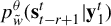
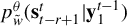
The predictive density given r periods of regimes is imposed to be

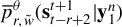
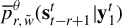
$\overline {p}_r^\theta (y_t|\mathbf {y}_1^{t-1},\mathbf {s}_{t-r+1}^t)$
 approximates the exact predictive density in two aspects. First, the exact distribution of
$y_t$
 conditional on
$(\mathbf {y}_1^{t-1},\mathbf {s}_{t-r+1}^t)$
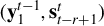 is a Gaussian mixture, while we impose the Gaussian density function in (21). Moreover, owing to the non-Gaussianity of
$x_t|(\mathbf {y}_1^{t},\mathbf {s}_{t-r+1}^t)$
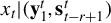 , the outputs
$\overline {y}^\theta _{t|t-1}(\mathbf {s}_{t-r+1}^t)$
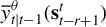 and
$\overline {\Omega }^\theta _{t|t-1}(\mathbf {s}_{t-r+1}^t)$
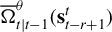 do not give the exact conditional mean and variance. We put
$\overline {y}^\theta _{t|t-1}(\mathbf {s}_{t-r+1}^t)$
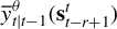 and
$\overline {\Omega }^\theta _{t|t-1}(\mathbf {s}_{t-r+1}^t)$
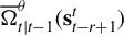 in (21) in place of the true conditional mean and variance.
Now that
$\overline {p}_r^\theta (y_t|\mathbf {y}_1^{t-1},\mathbf {s}_{t-r+1}^t)$
 and
$p_\theta (s_t|s_{t-1})$
 are ready, the algorithm in Hamilton (Reference Hamilton1989) can be applied to compute the likelihood function. Due to the potential difficulty in obtaining the closed-form expression of the stationary distribution, we use the conditional likelihood function given the initial latent variables
$(x_0,s_0)=(\tilde {x},\tilde {s})$
 . The choice of
$\tilde {x}$
 and
$\tilde {s}$
 can be arbitrary. In Section 4, we show the asymptotic properties of MLE with any choice of
$\tilde {x}$
 and
$\tilde {s}$
 , even if they are not the true underlying state and regime. The complete algorithm is stated as follows. For initialization,
$\overline {x}_{0|0}^\theta =\tilde {x}$
 and
$\overline {\Omega }_{0|0}^\theta =0$
 ,
$\overline {p}_r^\theta (s_0=\tilde {s})=1$
 , and
$\overline {p}_r^\theta (s_0=i)=0$
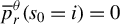 for
$i\neq \tilde {s}$
 . For
$t=1,2,\ldots ,n$
 ,
-
Step I. Calculate $\overline {p}_{r}^\theta (\mathbf {s}_{t-r+1}^t|\mathbf {y}_1^{t-1})=p_\theta (s_t|s_{t-1})\overline {p}_{r}^\theta (\mathbf {s}_{t-r+1}^{t-1}|\mathbf {y}_1^{t-1})$
 , where
$p_\theta (s_t|s_{t-1})$
is given by the transition matrix
$(q_{ij})$
, and
$\overline {p}_{r}^\theta (\mathbf {s}_{t-r+1}^{t-1}|\mathbf {y}_1^{t-1})$
is given by the initialization
$\overline {p}^\theta _r(s_0)$
for
$t=1$
and the previous Step V for
$t\geq 2$
.
-
Step II. Apply (12)–(17). Use the outputs to compute $\overline {p}_{r}^\theta (y_t|\mathbf {y}_1^{t-1},\mathbf {s}_{t-r+1}^t)$
according to (21). -
Step III. Calculate $\overline {p}_{r}^\theta (y_t|\mathbf {y}_1^{t-1})=\sum _{s_t,\dots ,s_{t-r+1}}\overline {p}_{r}^\theta (y_t|\mathbf {y}_1^{t-1},\mathbf {s}_{t-r+1}^t)\overline {p}_{r}^\theta (\mathbf {s}_{t-r+1}^t|\mathbf {y}_1^{t-1})$
, where
$\overline {p}_{r}^\theta (y_t|\mathbf {y}_1^{t-1},\mathbf {s}_{t-r+1}^t)$
is given by II, and
$\overline {p}_{r}^\theta (\mathbf {s}_{t-r+1}^t|\mathbf {y}_1^{t-1})$
is given by Step I. -
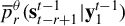
Step IV. Calculate $\overline {p}_{r}^\theta (\mathbf {s}_{t-r+1}^t|\mathbf {y}_1^{t})=\frac {\overline {p}_{r}^\theta (y_t|\mathbf {y}_1^{t-1},\ \mathbf {s}_{t-r+1}^t)\overline {p}_{r}^\theta (\mathbf {s}_{t-r+1}^t|\mathbf {y}_1^{t-1})}{\overline {p}_{r}^\theta (y_t|\mathbf {y}_1^{t-1})}$
, where
$\overline {p}_{r}^\theta (y_t|\mathbf {y}_1^{t-1},\mathbf {s}_{t-r+1}^t)$
is given by Step III,
$\overline {p}_{r}^\theta (\mathbf {s}_{t-r+1}^t|\mathbf {y}_1^{t-1})$
is given by Step I, and
$\overline {p}_{r}^\theta (y_t|\mathbf {y}_1^{t-1})$
is given by Step III. -
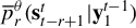
Step V. Calculate $\overline {p}_{r}^\theta (\mathbf {s}_{t-r+2}^{t}|\mathbf {y}_1^{t})=\sum _{s_{t-r+1}}\overline {p}_{r}^\theta (\mathbf {s}_{t-r+1}^t|\mathbf {y}_1^{t})$
and
$\overline {p}_{r,\tilde {x}}^\theta (s_{t-r+1}|\mathbf {y}_1^{t},\mathbf {s}_{t-r+2}^{t})=\frac {\overline {p}_{r,\tilde {x}}^\theta (\mathbf {s}_{t-r+1}^t|\mathbf {y}_1^{t})}{\overline {p}_{r,\tilde {x}}^\theta (\mathbf {s}_{t-r+2}^{t}|\mathbf {y}_1^{t})}$
. -
Step VI. Apply (18) and (20) with the outputs in Steps II, IV, and V.










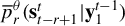



Let
$\tilde {w}=(\tilde {x},\tilde {s})$
 . We use the subscript
$\tilde {w}$
 to denote the initialization. The approximate log-likelihood function is

where
$\overline {p}_{r,\tilde {w}}^\theta (y_t|\mathbf {y}_1^{t-1})$
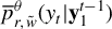 is obtained in Step III. The approximate MLE
$\hat {\theta }^{(r)}_{n,\tilde {w}}=\mathrm{arg\,max}_{\theta \in \Theta }\overline {\ell }^{(r)}_{n,\tilde {w}}(\theta )$
 .
3 PERFORMANCE OF THE APPROXIMATION ALGORITHM
In this section, we derive explicit expressions for the exact and approximate likelihood functions, analyze their difference, and build an upper bound for the approximation error.
3.1 Expressions of Exact and Approximate Likelihood Functions
This section derives the expressions for the exact and approximate likelihood functions, from which we can analyze their difference explicitly. The exact likelihood function conditional on the initial latent variables is

where

The approximate likelihood function can be expressed as

where
$\overline {p}_{r,\tilde {w}}^\theta (y_t|\mathbf {y}_1^{t-1},\mathbf {s}_{t-r+1}^t)$
 is given in (21). (24) can be derived by expanding the approximation algorithm step by step. More specifically,


where (25) follows from Step III, (26) follows by applying Steps I and V, and (27) follows from Step IV. If we continue to apply Steps I, V, and IV to
$\overline {p}_{r,\tilde {w}}^\theta (\mathbf {s}_{n-r}^{n-1}|\mathbf {y}_1^{n-2})$
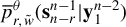 , then the likelihood function can be written as

If we repeat Steps I, V, and IV until
$t=1$
 , then (24) follows.
A close look at (22) and (24) shows that the difference in the two likelihood functions arises from the difference between
$p^\theta _{\tilde {w}}(y_t|\mathbf {y}_1^{t-1},\mathbf {s}_1^t)$
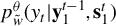 and
$\overline {p}^\theta _{r,\tilde {w}}(y_t|\mathbf {y}_1^{t-1},\mathbf {s}_{t-r+1}^t)$
 for
$t\geq r+1$
 . Section 3.2 theoretically derives an upper bound of the difference.
3.2 Difference between Exact and Approximate Likelihood Functions
This section bounds the approximation error. Let
$\Theta $
 denote the parameter space. For a given
$\theta \in \Theta $
 , let
$\alpha _j(\theta )$
 denote the
$\alpha _j$
 -component of
$\theta $
 . For
$i\in \mathbb S$
 and
$j=1,\ldots ,J-1$
 , let
$q_{ij}(\theta )$
 denote the
$q_{ij}$
 -component of
$\theta $
 , and define
$q_{iJ}(\theta )=1-\sum _{\ell =1}^{J-1}q_{i\ell }(\theta )$
 . Define
$\alpha _{\max }(\theta )\triangleq \max _{j\in \mathbb S}|\alpha _j(\theta )|$
 as the maximum of the absolute values of the
$\alpha _j$
 -components across regimes under
$\theta $
 , and
$\alpha _+\triangleq \textrm {sup}_{\theta \in \Theta }\alpha _{\max }(\theta )$
 as the supremum of this quantity over all parameter values in
$\Theta $
 .
Assumption 2. The parameter
$\theta $
 belongs to
$\Theta $
 .
$\Theta $
 is compact.
$\theta _0$
 lies in the interior of
$\Theta $
 .
Assumption 3.
$\inf _{\theta \in \Theta } \min _{i,j\in \mathbb {S}} q_{ij}(\theta )>0$
 .
Assumption 4.
$\alpha _+=\textrm {sup}_{\theta \in \Theta }\max _{j\in \mathbb {S}}|\alpha _j(\theta )|<1$
 .
Throughout the article, we work on stationary and ergodic
$(x_t,s_t,y_t)$
 .
Lemma 1. Suppose it holds that
$\min _{i,j\in \mathbb {S}}q_{ij}(\theta _0)>0$
 and
$\max _{j\in \mathbb {S}}|\alpha _j(\theta _0)|<1$
 . Then (1) and (2) admit a unique stationary and ergodic solution. This solution also satisfies
$\mathbb {E}_0 y_t^8<\infty $
 .
As stated at the end of Section 3.1, the difference between the approximate and exact likelihood functions arises from the difference in
$p^{\theta }_{\tilde {w}}(y_t|\mathbf {y}_1^{t-1},\mathbf {s}_1^t)$
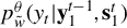 and
$\overline {p}^{\theta }_{r,\tilde {w}}(y_t|\mathbf {y}_1^{t-1},\mathbf {s}_{t-r+1}^t)$
 . Because both
$p^{\theta }_{\tilde {w}}(y_t|\mathbf {y}_1^{t-1},\mathbf {s}_1^t)$
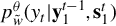 and
$\overline {p}^{\theta }_{r,\tilde {w}}(y_t|\mathbf {y}_1^{t-1},\mathbf {s}_{t-r+1}^t)$
 take the form of Gaussian densities, their difference comes from what we put in the places of means and variances or, more specifically,
$\bar {y}^{\theta }_{t|t-1}(\mathbf {s}_{t-r+1}^t)-y^{\theta }_{t|t-1}(\mathbf {s}_1^t)$
 and
$\overline {\Sigma }^{\theta }_{t|t-1}(\mathbf {s}_{t-r+1}^t)-\Sigma ^{\theta }_{t|t-1}(\mathbf {s}_1^t)$
 . Define

From (6), (8), (13), and (15),

Then it suffices to derive the upper bounds of
$|\Delta _{r,t}^x(\mathbf {s}_1^t;\theta )|$
 and
$|\Delta _{r,t}^\Omega (\mathbf {s}_1^t;\theta )|$
 . We first give the following lemma useful for understanding the derivation.
Lemma 2. Assume Assumptions 1–4. During the application of the Kalman filter (5)–(10), for one sequence of iterations
$x^{\theta }_{t|t}(\mathbf {s}_{1}^{t})$
 and
$\Omega ^{\theta }_{t|t}(\mathbf {s}_{1}^{t})$
 starting from
$x_{0|0}^\theta $
 and
$\Omega _{0|0}^\theta $
 and another sequence
$\check {x}_{t|t}^\theta (\mathbf {s}_{1}^{t})$
 and
$\check {\Omega }_{t|t}^\theta (\mathbf {s}_{1}^{t})$
 starting from
$\check {x}_{0|0}^\theta $
 and
$\check {\Omega }_{0|0}^\theta $
 , there exists a sequence of positive random variables
$\xi _t$
 and constants
$c_\xi $
 and c such that, for all
$t=1,2,\ldots $
 ,
$\mathbb {E}_{0}\xi _t^2\leq c_\xi $
 , and for all
$\theta \in \Theta $
 ,

Lemma 2 states that the Kalman filter is convergent. More specifically, for two sequences of Kalman filter iterations different only in their starting points, the difference in their outputs decays exponentially at the rate of
$\alpha _{\max }(\theta )$
 . Then we bound
$|\Delta _{r,t}^x(\mathbf {s}_1^t;\theta )|$
 and
$|\Delta _{r,t}^\Omega (\mathbf {s}_1^t;\theta )|$
 .
Theorem 1. Assume Assumptions 1–4. Constant
$c_\Delta>0$
 exists such that for any choice of initialization
$w_0=\tilde {w}$
 , there exist a constant
$c_M>0$
 and a sequence of positive random variables
$M_t$
 satisfying for all
$t\geq r$
 ,
$\mathbb {E}_0 \ \mathrm {sup}_{\theta \in \Theta } M_t^2<c_{M}$
 , and for all
$\theta \in \Theta $
 ,


We give the general idea of the proof of (29). The discrepancy at
$t-1$
 is
$\Delta _{r,t-1}^\Omega (\mathbf {s}_1^{t-1};\theta )$
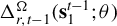 . Notice that, in spite of potentially different inputs, the prediction and update steps (12)–(17) in the approximation algorithm are the same as (5)–(10) in the Kalman filter. After the update step at time t,
$|\Delta _{r,t}^\Omega (\mathbf {s}_1^t;\theta )|\leq \alpha _{\max }(\theta )^2|\Delta _{r,t-1}^\Omega (\mathbf {s}_1^{t-1};\theta )|$
 , because the Kalman filter is convergent, as shown in Lemma 2. Then the collapsing step averages out the regime r periods ahead. The resulting difference is the discrepancy between the average and each path, which is bounded by the maximum difference between any two possible paths, differing only at the regime r periods ahead. It is reflected in (30):

From Lemma 2, (30) is bounded by

Then (29) follows from upper bounds of
$\Omega ^\theta _{t|t}(\mathbf {s}_1^t)$
 and iteration of the inequality. The proof of (28) follows the same idea.
Equipped with Theorem 1, we can show an upper bound of the approximation error.
Proposition 1. Assume Assumptions 1–4. Constant
$c>0$
 exists such that for any initialization
$w_0=\tilde {w}$
 , there exist constants
$c_M,c_N>0$
 and sequences of positive random variables
$M_t$
 and
$N_t$
 satisfying for all
$t\geq r$
 ,
$\mathbb {E}_0\ \mathrm {sup}_{\theta \in \Theta }M_t^2<c_M$
 ,
$\mathbb {E}_0\ \mathrm {sup}_{\theta \in \Theta }N_t<c_N$
 , and for all
$\theta \in \Theta $
 ,

Moreover,

Remark 2. Equation (31) bounds the approximation error at time t uniformly over all possible regime sequences. Inherited from Theorem 1, (31) increases with
$\alpha _{\max }(\theta )$
 and decreases with r. The bound in (32) for the log-likelihood, derived from (31), grows with n because the per-period approximation errors accumulate.
Kim and Kang (Reference Kim and Kang2019) used simulation to show that the approximation error is small when regimes are persistent. We provide an analytical explanation for this observation. When regimes are highly persistent and seldom switch, the likelihood is close to that of a single-regime state-space model, and the approximation error tends to be small. To see this analytically, note that the total approximation error can be decomposed across all possible regime paths. For persistent regimes, paths involving frequent regime switches carry low probability weights and thus contribute little to the overall error. The main contribution comes instead from paths where the regime remains invariant. For such a path with
$s_t=s$
 for all t, the approximation error for the filtered covariance matrix can be expressed as

In (33), the term
$\overline {p}_r^\theta (s_{t-r+1}=i|\mathbf {s}_{t-r+2}^t,\mathbf {y}_1^t)$
 is small for
$i\neq s$
 , so the overall approximation error remains small under high regime persistence. The same reasoning applies to the approximation error for the filtered mean. Thus, the approximation error is small.
Regime persistence does not enter the theoretical bound in Proposition 1 explicitly. This is because, when deriving this bound, we condition on the full regime path and compute the maximum bound across all paths. As a result, Proposition 1 provides a uniform bound that holds for any regime sequence, regardless of its persistence.
Our simulation study in Section A.3 of the Supplementary Material adds one further observation. Although the approximation error is small when regimes are persistent, this relationship is not necessarily monotonic. Under certain specifications, the error may initially increase before decreasing as regimes become more persistent.
3.3 Difference between Exact and Approximate Inferred Latent Variables
In MS state-space models,
$x_t$
 and
$s_t$
 cannot be directly observed and thus require inference. This section examines the difference between the latent variable inference based on the exact likelihood function and that based on the approximation algorithm. We consider three types of inferences for the regime and the state at time t: the predictive inference using the information up to time
$t-1$
 , the updated inference using the information up to time t, and the smoothed inference using the full sample. The approximate inference is explained in Kim (Reference Kim1994). For readers’ convenience, we explain the computation method before we introduce our main findings.
For the regime process, its predictive inference
$\{\overline {p}^{\theta }_{r,\tilde {w}}(s_t|\mathbf {y}_1^{t-1})\}_{1\leq t\leq n}$
 and updated inference
$\{\overline {p}^{\theta }_{r,\tilde {w}}(s_t|\mathbf {y}_1^{t})\}_{1\leq t\leq n}$
 can be obtained in Steps I and IV of the algorithm to compute the likelihood function. For the smoothed probability, when
$t=n$
 ,
$\overline {p}^{\theta }_{r,\tilde {w}}(\mathbf {s}_{n-r+1}^{n}|\mathbf {y}_1^{n})$
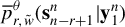 is the last entry of
$\{\overline {p}^{\theta }_{r,\tilde {w}}(\mathbf {s}_{t-r+1}^t|\mathbf {y}_1^{t})\}_{1\leq t\leq n}$
 obtained at Step IV. For
$t<n$
 ,
$\overline {p}^{\theta }_{r,\tilde {w}}(\mathbf {s}_{t-r+1}^t|\mathbf {y}_1^{n})$
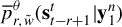 can be computed backward given
$\overline {p}^{\theta }_{r,\tilde {w}}(\mathbf {s}_{t-r+2}^{t+1}|\mathbf {y}_1^{n})$
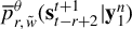 followingFootnote
1

Theorem 2 gives the findings about the exact and approximate inferred probabilities.
Theorem 2. Assume Assumptions 2–4. Constant
$c>0$
 exists such that for any choice of initialization
$w_0=\tilde {w}$
 , there exist constants
$c_M,c_N>0$
 and sequences of positive random variables
$M_t$
 and
$N_t$
 satisfying
$\mathbb {E}_0 \ \mathrm {sup}_{\theta \in \Theta } M_t^2<c_M$
 and
$\mathbb {E}_0\ \mathrm {sup}_{\theta \in \Theta } N_t<c_N$
 for all
$t\geq r$
 , and for all
$\theta \in \Theta $
 ,


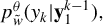
To show Theorem 2, we first derive the expressions of approximate inferred probabilities


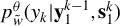
The derivation of the expressions essentially parallels the derivation of the approximate likelihood expression in Section 3.1 by the repeated application of Steps I, V, and IV. The details are deferred to the Supplementary Material. The expressions of the exact inferred probabilities can be obtained by replacing
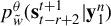
$\overline {p}^{\theta }_{r,\tilde {w}}(y_k|\mathbf {y}_1^{k-1},\mathbf {s}_{k-r+1}^{k})$
 and
$\overline {p}^{\theta }_{r,\tilde {w}}(y_k|\mathbf {y}_1^{k-1})$
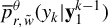 with
$p^{\theta }_{\tilde {w}}(y_k|\mathbf {y}_1^{k-1},\mathbf {s}_{1}^{k})$
 and
$p^{\theta }_{\tilde {w}}(y_k|\mathbf {y}_1^{k-1}),$
 respectively. Then Theorem 2 follows if we apply Proposition 1.
Next, we explain the state inference algorithm. Let
$x_{t|k}^{\theta }$
 and
$\overline {x}_{t|k}^{(r,\theta )}$
 denote the exact and approximate inference about the state given
$\{y_k,\ldots ,y_1,x_0,s_0\}$
 , respectively. We might omit the superscript
$(r)$
 and simply write
$\overline {x}^{\theta }_{t|k}$
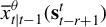
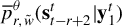
 when there is no confusion. The approximate predictive and updated inference can be computed from

where
$\overline {x}^{\theta }_{t|t-1}(\mathbf {s}_{t-r+1}^t)$
 and
$\overline {x}^{\theta }_{t|t}(\mathbf {s}_{t-r+2}^{t})$
 can be obtained from (12) and (18), and
$\overline {p}^{\theta }_{r,\tilde {w}}(\mathbf {s}_{t-r+1}^t|\mathbf {y}_1^{t-1})$
 and
$\overline {p}^{\theta }_{r,\tilde {w}}(\mathbf {s}_{t-r+2}^{t}|\mathbf {y}_1^{t})$
 can be obtained in Steps I and IV. For the smoothed inference, when
$t=n$
 ,
$\overline {x}^{\theta }_{n|n}(\mathbf {s}_{n-r+2}^n)$
 can be obtained from (18). For
$t<n$
 ,

where
$\overline {x}^{\theta }_{t|n}(\mathbf {s}_{t-r+2}^{t})$
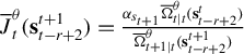
 can be computed backward following

where
$\overline {J}^{\theta }_t(\mathbf {s}_{t-r+2}^{t+1})=\frac {\alpha _{s_{t+1}}\overline {\Omega }^{\theta }_{t|t}(\mathbf {s}_{t-r+2}^{t})}{\overline {\Omega }^{\theta }_{t+1|t}(\mathbf {s}_{t-r+2}^{t+1})}$
 . The difference between exact and approximate inference of
$x_t$
 can be summarized as follows.
Theorem 3. Assume Assumptions 1–4. Constant
$c_\Delta>0$
 exists such that for any choice of initialization
$w_0=\tilde {w}$
 , there exist constants
$c_{n},c_{N},c_{M},c_A>0$
 and sequences of positive random variables
$\{n_t\}_{t\geq 1}$
 ,
$\{M_t\}_{t\geq 1}$
 ,
$\{N_t\}_{t\geq 1}$
 , and
$\{A_{t,k}\}_{t\geq 1,k\geq 1}$
 satisfying
$\mathbb {E}_0\ \mathrm {sup}_{\theta \in \Theta }n_t^2<c_{n}$
 ,
$\mathbb {E}_0\ \mathrm {sup}_{\theta \in \Theta }N_t^2<c_{N}$
 ,
$\mathbb {E}_0\ \mathrm {sup}_{\theta \in \Theta }M_t^4<c_{M}$
 , and
$\mathbb {E}_0\ \mathrm {sup}_{\theta \in \Theta }\ A_{t,k}\leq c_{A}$
 for all
$t,k\geq 1$
 , and for all
$\theta \in \Theta $
 ,


4 ASYMPTOTIC PROPERTIES OF THE APPROXIMATE MLE
In this section, we let r depend on the sample size n,
$r=r_n$
 . We show consistency and asymptotic normality of the approximate MLE, if
$r_n$
 increases with n at an appropriate rate, and give consistent estimates of the asymptotic covariance matrix. The proof consists of two parts. We first show in Section 4.1 the asymptotic properties of the exact MLE
$\tilde {\theta }_{n,\tilde {w}}=\mathrm{arg\,max}_{\theta \in \Theta } \ell _{n,\tilde {w}}(\theta )$
 , where

with
$p^\theta _{\tilde {w}}(y_1,\dots ,y_n)$
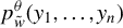 in (22). Section 4.2 shows that the exact MLE
$\tilde {\theta }_{n,\tilde {w}}$
 and the approximate MLE
${\hat {\theta }}_{n,\tilde {w}}^{(r_n)}$
 share the same asymptotic properties if
$r_n$
 increases with n to infinity at a proper rate.
4.1 Asymptotic Properties of the Exact MLE
The asymptotic properties of the exact MLE relate to the literature of hidden Markov models. The MS state-space model belongs to the class of hidden Markov models because the latent process
$(x_t,s_t)$
 is a Markov chain, and given
$(x_t,s_t)$
 ,
$(y_t)$
 is a sequence of conditionally independent random variables. Consistency follows from Douc and Moulines (Reference Douc and Moulines2012), which shows the consistency of the MLE in a wide range of hidden Markov models.
Theorem 4. Assume Assumptions 1–4. Then, for any
$\tilde {w}\in \mathbb {W}$
 ,
$\lim _{n\rightarrow \infty } \tilde {\theta }_{n,\tilde {w}}=\theta _0$
 ,
$\mathbb {P}_0$
 -a.s.
Asymptotic normality of the exact MLE follows from a central limit theorem for the Fisher score function

and a locally uniform law of large numbers for the observed Fisher information

The summands in (44) and (45) do not form stationary ergodic sequences, because
$p_{\theta ,\tilde {w}}(y_t|\mathbf {y}_1^{t-1})$
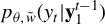 depends on the accumulating
$\mathbf {y}_1^{t-1}$
 . Thus, we cannot directly apply the law of large numbers or the central limit theorem. The strategy, originated from Baum and Petrie (Reference Baum and Petrie1966), is to approximate the summands with stationary ergodic sequences. Bickel et al. (Reference Bickel, Ritov and Rydén1998), Jensen and Petersen (Reference Jensen and Petersen1999), Douc et al. (Reference Douc, Moulines and Rydén2004), Kasahara and Shimotsu (Reference Kasahara and Shimotsu2019), Pouzo et al. (Reference Pouzo, Psaradakis and Sola2022), and Li and Liu (Reference Li and Liu2023) then take this approach. A key step in their approximation is that the upper bounds of the difference between the summands and stationary ergodic sequences involve

$j=1,2$
 . Because they assumed that
$\textrm {sup}_{w_{k-1},w_k} |\nabla _\theta ^j\log p_\theta (y_k,w_k|w_{k-1})|$
 is bounded and that
$\frac {\inf _{\theta }\inf _{w_{k-1},w_k}p_\theta (w_k|w_{k-1})}{\textrm {sup}_\theta \textrm {sup}_{w_{k-1},w_k}p_\theta (w_k|w_{k-1})}>0$
 , the difference decays exponentially with k. For MS state-space models, however,
$\textrm {sup}_{w_{k-1},w_k} |\nabla _\theta ^j\log p_\theta (y_k,w_k|w_{k-1})|=+\infty $
 and
$\inf _{\theta }\inf _{w_{k-1},w_k}p_\theta (w_k|w_{k-1})=0$
 , and these two assumptions no longer hold. Thus, the previous results do not apply in this study.
We contribute to the literature by showing asymptotic normality of the exact MLE in MS state-space models. Two instruments play an important role in showing the approximation. The first one is the exponential forgetting of the filtering distribution established by Douc and Moulines (Reference Douc and Moulines2012, Prop. 5). It imposes a much less stringent assumption on the transition density and only requires a positive lower bound on a large enough set, which holds in MS state-space models. The second instrument is the relaxed upper bound of the score function and Hessian. We show that the score function and Hessian at each period are bounded above by random variables with finite second moments, which suffices to show the approximation in probability. With these two instruments combined, we can show the influence of the information far in the past vanishes quickly. Then the original sequences can be approximated with the stationary sequences starting from past infinity. Next, we introduce the notation and present the two instruments in Lemmas 3 and 4.
Because our subsequent analysis involves operations on transition kernels, we first recall the notation for these operations on a generic measurable space. Let
$(\mathsf {X}, \mathcal {X})$
 be an arbitrary measurable space, and let L be a transition kernel on
$(\mathsf {X}, \mathcal {X})$
 . That is, for any
$x \in \mathsf {X}$
 ,
$L(x, \cdot )$
 is a finite measure on
$(\mathsf {X}, \mathcal {X}),$
 and for any
$A \in \mathcal {X}$
 ,
$x \mapsto L(x, A)$
 is measurable function from
$(\mathsf {X}, \mathcal {X})$
 to
$([0, 1], \mathcal {B}([0, 1]))$
 . L acts on bounded functions f on
$\mathsf {X}$
 and on
$\sigma $
 -finite positive measures
$\mu $
 on
$(\mathsf {X}, \mathcal {X})$
 via

If
$L_1$
 and
$L_2$
 are two transition kernels on
$(\mathsf {X}, \mathcal {X})$
 , then
$L_1 L_2$
 is the transition kernel on
$(\mathsf {X}, \mathcal {X})$
 , given, for any
$x \in \mathsf {X}$
 and
$A \in \mathcal {X}$
 by

For the MS state-space model, let
$w_t=(x_t,s_t)'$
 denote the latent process taking values on
$\mathbb {W}=\mathbb {R}\times \mathbb {S}$
 and with the associated Borel
$\sigma $
 -field
$\mathcal {W}=\mathcal {B}(\mathbb {R}\times \mathbb {S})$
 , and
$\varpi $
 denote the product measure of Lebesgue measure and counting measure on
$(\mathbb {W},\mathcal {W})$
 . We use
$g_\theta (y_t|w_t)$
 to denote the conditional density of
$y_t$
 given
$w_t$
 . We use
$\mathcal {H}_\theta (w,A)$
 with
$w\in \mathbb {W}$
 and
$A\in \mathcal {W}$
 to denote the transition kernel of the Markov process
$w_t$
 . Let
$h_\theta (w,\cdot )$
 denote the density of
$\mathcal {H}_\theta (w,\cdot )$
 with respect to
$\varpi $
 . We follow Douc and Moulines (Reference Douc and Moulines2012) and define the unnormalized kernel

for
$w_{-m}\in \mathbb {W}$
 and
$A\in \mathcal {W}$
 . We use
$\phi _{\theta ,k}$
 as the shorthand notation of

and use
$\dot {\phi }_{\theta ,k}$
 as the shorthand notation of

Lemma 3 (Proposition 5 in Douc and Moulines, Reference Douc and Moulines2012).
Assume Assumptions 1–4. Let
$0\leq \gamma ^-< \gamma ^+\leq 1$
 . There exists a
$\mathbb {P}_0$
 -a.s. finite random variable K such that for any
$\eta>0$
 , there exists
$\rho \in (0,1)$
 satisfying

for any
$k+m\geq K$
 , any
$\gamma \in (\gamma ^-,\gamma ^+)$
 , any bounded function
$\mathrm {f}$
 and any nonnegative bounded function
$\mathrm {g}$
 , any probability measure
$\xi $
 and
$\xi '$
 on
$(\mathbb {W},\mathcal {W}),$
 and any
$\theta \in \Theta $
 .
The left-hand side of (48) is the difference between two variables starting from distinct initial distributions
$\xi $
 and
$\xi '$
 . Because we can set
$\rho ,\eta \in (0,1)$
 , Lemma 3 states that the influence of the initial distributions decays geometrically if the random variables on the right-hand side of (48) can be bounded properly. Douc et al. (Reference Douc, Moulines and Rydén2004, Cor. 1), Kasahara and Shimotsu (Reference Kasahara and Shimotsu2019, Lem. 1), Pouzo et al. (Reference Pouzo, Psaradakis and Sola2022, Thm. 2), and Li and Liu (Reference Li and Liu2023, Lem. 3.1) serve the same function. They assumed
$\frac {\inf _{\theta }\inf _{w_{k-1},w_k}h_\theta (w_{k-1},w_k)}{\textrm {sup}_\theta \textrm {sup}_{w_{k-1},w_k}h_\theta (w_{k-1},w_k)}>0$
 and that the decaying rate is
$1-\frac {\inf _{\theta }\inf _{w_{k-1},w_k}h_\theta (w_{k-1},w_k)}{\textrm {sup}_\theta \textrm {sup}_{w_{k-1},w_k}h_\theta (w_{k-1},w_k)}<1$
 . Their rate does not apply here because
$x_t$
 takes values on the entire real line and
$\inf _{\theta }\inf _{w_{k-1},w_k}p_\theta (w_k|w_{k-1})=0$
 . Lemma 3 extends the previous results. It considers the difference on a compact set C and its complement separately. The decaying rate on C is
$\rho \triangleq 1-\frac {\inf _{\theta }\inf _{w_{k-1},w_k\in C}h_\theta (w_{k-1},w_k)^2}{\textrm {sup}_\theta \textrm {sup}_{w_{k-1},w_k\in C}h_\theta (w_{k-1},w_k)^2}<1$
 , which parallels the previous results. To control the difference on C’s complement, it is assumed
$\textrm {sup}_{w\in C^c}g_\theta (y|w)<\eta \textrm {sup}_{w\in \mathbb {W}}g_\theta (y|w)$
 for all
$\theta $
 and y. This assumption is satisfied if C is chosen to be large enough. The decaying rate on C’s complement is
$\eta $
 , which extends the previous results to noncompact sets.
Lemma 4. Assume Assumptions 1–4. There exist random variables
$U_k\in L(\mathbb {P}_0)$
 such that for
$-m+1\leq k\leq t$
 and any
$\tilde {w}=(\tilde {x},\tilde {s})\in \mathbb {W}$
 ,
-
(a) $\mathrm{sup}_{\theta \in \Theta }\mathbb {E}_\theta [|\phi _{\theta ,k}|^2\,| \mathbf {y}_{-m+1}^t]\!\!\leq U_k$
,
$\mathrm {sup}_{\theta \in \Theta }\mathbb {E}_\theta [|\phi _{\theta ,k}|^2\,| \mathbf {y}_{-m+1}^t,w_{-m}\!\!\!=\tilde {w}]\leq c\alpha _+^{2(k+m-1)}\tilde {x}^2+U_k$
; -
(b) $\mathrm {sup}_{\theta \in \Theta }\mathbb {E}_\theta [|\dot {\phi }_{\theta ,k}|\,| \mathbf {y}_{-m+1}^t]\leq U_k$
,
$\mathrm {sup}_{\theta \in \Theta }\mathbb {E}_\theta [|\dot {\phi }_{\theta ,k}|\,| \mathbf {y}_{-m+1}^t,w_{-m}=\tilde {w}]\leq c\alpha _+^{2(k+m-1)}\tilde {x}^2+U_k$
.




Lemma 4 shows the relaxed upper bounds of the period score function and Hessian. We need the following additional assumptions.
Assumption 5. Constant
$\delta>0$
 exists such that on
$G\triangleq \{\theta \in \Theta :|\theta -\theta _0|<\delta \}$
 ,
-
(a) $\mathbb {E}_0[\textrm {sup}_{m\geq 0}\textrm {sup}_{\theta \in G}|\nabla _\theta \log p_\theta (y_1|\mathbf {y}_{-m+1}^0)|^2]<\infty $
; -
(b) $\mathbb {E}_0[\textrm {sup}_{m\geq 0}\textrm {sup}_{\theta \in G}|\nabla _\theta ^2\log p_\theta (y_1|\mathbf {y}_{-m+1}^0)|]<\infty $
; -
(c) for any $\tilde {w}\in \mathbb {W}$
,
$\mathbb {E}_0[\textrm {sup}_{m\geq 0}\textrm {sup}_{\theta \in G}|\nabla _\theta \log p_\theta (y_1|\mathbf {y}_{-m+1}^0,w_{-m}=\tilde {w})|^2]<\infty $
; -
(d) for any $\tilde {w}\in \mathbb {W}$
,
$\mathbb {E}_0[\textrm {sup}_{m\geq 0}\textrm {sup}_{\theta \in G}|\nabla _\theta ^2\log p_\theta (y_1|\mathbf {y}_{-m+1}^0,w_{-m}=\tilde {w})|]<\infty $
.






We need the high-level Assumption 5 to show the approximation in
$L^p$
 . In the special cases of bounded state space, Douc et al. (Reference Douc, Moulines and Rydén2004), Pouzo et al. (Reference Pouzo, Psaradakis and Sola2022), and Li and Liu (Reference Li and Liu2023) could show Assumption 5 with verifiable assumptions. In our model with a non-compact state space, Lemmas 3 and 4 help to show the approximation only in probability.
4.1.1 A Central Limit Theorem for the Score Function
This section shows asymptotic normality of the score function. First, we show that the score function can be approximated by a sequence of integrable martingale increments. Using the Fisher identity,Footnote 2 which states that the score function of a model with missing data equals the conditional expectation of the complete score given the observed data, the score function can be written as

where

We can similarly define the period score function that starts from the stationary initial distribution

Lemma 5 shows that the difference in the period score function with different starting points diminishes at a geometric rate. It parallels Douc et al. (Reference Douc, Moulines and Rydén2004, Lem. 8), Kasahara and Shimotsu (Reference Kasahara and Shimotsu2019, Lem. 4), Pouzo et al. (Reference Pouzo, Psaradakis and Sola2022, Lem. 7), and Li and Liu (Reference Li and Liu2023, Lem. 5.1). In their theories, the decaying rate
$\tilde {\rho }=1-\frac {\inf _{\theta }\inf _{w_{k-1},w_k}h_\theta (w_{k-1},w_k)}{\textrm {sup}_\theta \textrm {sup}_{w_{k-1},w_k}h_\theta (w_{k-1},w_k)}$
 is assumed to be strictly smaller than unity. For MS state-space models,
$\inf _{\theta }\inf _{w_{k-1},w_k}h_\theta (w_{k-1},w_k)=0$
 , and thus
$\tilde {\rho }=1$
 , the difference is non-decaying, and the previous theories no longer apply. We use Lemmas 3 and 4 to establish the geometric decaying rate. More specifically, we write (49) and (50) when
$m=0,$
 respectively, as

for
$3\leq k\leq t$
 , where
$\chi =\mathbb {P}_\theta (w_1\in A|w_0=\tilde {w})$
 ,
$\overline {\chi }$
 denotes the stationary distribution of
$w_t$
 ,


Then Lemma 3 provides an upper bound of
$\big |\mathbb {E}_\theta [\phi _{\theta ,k}|\mathbf {y}_{1}^t,w_{0}=\tilde {w}]-\mathbb {E}_\theta [\phi _{\theta ,k}|\mathbf {y}_{1}^t]\big |$
 , which leads to the upper bound of
$|\Phi _{t,0,\tilde {w}}(\theta _0)-\Phi _{t,0}(\theta _0)|$
 in Lemma 5(a). Because
$\rho ,\eta \in (0,1)$
 in Lemma 3, the difference is decaying geometrically as k increases. Lemma 4 helps bound the other terms on the right-hand side of (48). Lemma 5(b) follows similarly.
Lemma 5. Assume Assumptions 1–5. Then there exist constants
$\varrho \in (0,1)$
 ,
$c>~0,$
 and a random variable
$B\in L^2(\mathbb {P}_0)$
 such that for some
$\mathbb {P}_0$
 -a.s. finite random variable K,
-
(a) $|\Phi _{t,0,\tilde {w}}(\theta _0)-\Phi _{t,0}(\theta _0)|\leq \varrho ^t(t^2B+c\tilde {x})$
,
$\mathbb {P}_0$
-a.s. for
$t>K$
and any
$\tilde {w}\in \mathbb {W}$
; -
(b) $|\Phi _{t,m}(\theta _0)-\Phi _{t,m'}(\theta _0)| \leq Bt^2(m^2+1)\varrho ^{t+m}$
,
$\mathbb {P}_0$
-a.s. for
$t+m>K$
and
$m'\geq m $
.






Lemma 5 implies that
$\{\Phi _{t,m}(\theta _0)\}_{m\geq 0}$
 is a Cauchy sequence and converges to
$\Phi _{t,\infty }(\theta _0)\triangleq \lim _{m\rightarrow \infty }\Phi _{t,m}(\theta _0)$
 . Define the filtration
$\mathcal {F}_t=\sigma (y_k,-\infty < k\leq t)$
 . From Assumption 5, Durrett (Reference Durrett2019, Exer. 2.3.7 and Thm. 5.5.9), and
$\mathbb {E}_0[\Phi _{t,m}(\theta _0)|\mathbf {y}_{-m+1}^{t-1}]=0$
 , it follows that
$\mathbb {E}_0[\Phi _{t,\infty }(\theta _0)|\mathbf {y}_{-\infty }^{t-1}]=0$
 and
$I(\theta _0)\triangleq \mathbb {E}_{0}[\Phi _{t,\infty }(\theta _0)\Phi _{t,\infty }(\theta _0)^T]<\infty $
 . Therefore,
$\{\Phi _{t,\infty }(\theta _0)\}_{t=-\infty }^\infty $
 is an
$(\mathcal {F},\mathbb {P}_0)$
 -adapted stationary ergodic and square integrable martingale increment sequence. The central limit theorem implies
$n^{-\frac {1}{2}}\sum _{t=1}^n\Phi _{t,\infty }(\theta _0)\Rightarrow \mathbb {N}(0,I(\theta _0))$
 .
Because the influence of the initial distribution decays geometrically, as shown in Lemma 5,
$\Phi _{t,0,\tilde {w}}(\theta )$
 can be approximated with
$\Phi _{t,\infty }(\theta )$
 , which is summarized in Lemma 6.
Lemma 6. Assume Assumptions 1–5. Then, for any
$\tilde {w}\in \mathbb {W}$
 ,

Then
$n^{-\frac {1}{2}}\sum _{t=1}^n\Phi _{t,0,\tilde {w}}(\theta _0)$
 has the same limiting distribution as
$n^{-\frac {1}{2}}\sum _{t=1}^n\Phi _{t,\infty }(\theta _0)$
 . The score function is asymptotically normally distributed.


4.1.2 Law of Large Numbers for the Observed Fisher Information
This section presents the law of large numbers for the observed Fisher information. Using Louis missing information principle,Footnote 3 we write

with
$\dot {\phi }_{\theta ,t}$
 defined in (47). Similar to Section 4.1.1, we first approximate the Hessian with a stationary ergodic sequence. The proof parallels that in Section 4.1.1 and we defer the details to the Supplementary Material.
Theorem 6. Assume Assumptions 1–5. Let
$\{\theta _n^*\}$
 be any, possibly stochastic, sequence in
$\Theta $
 such that
$\theta _n^*\overset {a.s.}{\rightarrow }\theta _0$
 . Then, for any
$\tilde {w}\in \mathbb {W}$
 ,
$-n^{-1}\nabla _\theta ^2\ell _{n,\tilde {w}}(\theta _n^*)\overset {a.s.}{\rightarrow }I(\theta _0)$
 .
Theorems 5 and 6 together provide the following theorem of asymptotic normality.



4.2 Asymptotic Properties of the Approximate MLE
This section establishes the asymptotic properties of the approximate MLE and provides a consistent estimate of the asymptotic covariance matrix. We first show in Theorems 8 and 9 that the normalized likelihood function, score function, and Hessian matrix converge to the exact ones uniformly if
$r_n$
 increases at proper rates with n. Then Theorem 10 establishes the asymptotic normality of the approximate MLE and consistency of the asymptotic covariance matrix estimates.
Theorem 8 shows that the difference between the normalized approximate likelihood and the exact one diminishes to zero. Moreover, a larger
$\alpha _+$
 requires
$r_n$
 to grow at a faster rate.
Theorem 8. Assume Assumptions 1–4. If
$r_n$
 satisfies
$\alpha _+^{r_n}\rightarrow 0$
 as
$n\rightarrow \infty $
 , then for any initial
$\tilde {w}$
 ,

As stated in Section 3.2, the discrepancy between the approximate and exact likelihood functions arises essentially from
$\overline {x}_{t|t}^\theta (\mathbf {s}_{t-r+2}^{t})-x_{t|t}^\theta (\mathbf {s}_1^t)$
 and
$\overline {\Omega }_{t|t}^\theta (\mathbf {s}_{t-r+2}^{t})-\Omega _{t|t}^\theta (\mathbf {s}_1^t)$
 . Then the difference between the approximate and exact score functions (resp. Hessian matrices) comes from the first (resp. second) order derivatives of
$\overline {x}_{t|t}^\theta (\mathbf {s}_{t-r+2}^{t})-x_{t|t}^\theta (\mathbf {s}_1^t)$
 and
$\overline {\Omega }_{t|t}^\theta (\mathbf {s}_{t-r+2}^{t})-\Omega _{t|t}^\theta (\mathbf {s}_1^t)$
 . Define

Their upper bounds are shown in Lemma 7.
Lemma 7. Assume Assumptions 1–5. Constant
$c>0$
 exists such that for any choice of initialization
$w_0=\tilde {w}$
 , there exist constants
$c_{\tilde {M}},c_{\tilde {\tilde {M}}}$
 and sequences of positive random variables
$M_t$
 ,
$\tilde {M}_t$
 , and
$\tilde {\tilde {M}}_t$
 satisfying for all
$t\geq r$
 ,
$\mathbb {E}_0\mathrm {sup}_{\theta \in \Theta } M_t^4<c_{\tilde {M}}$
 ,
$\mathbb {E}_0\mathrm {sup}_{\theta \in \Theta }\tilde {M}_t^4<c_{\tilde {M}}$
 ,
$\mathbb {E}_0\mathrm {sup}_{\theta \in \Theta }\tilde {\tilde {M}}_t^4<c_{\tilde {\tilde {M}}}$
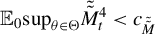 , and for all
$\theta \in \Theta $
 ,


Building on Lemma 7, we derive the convergence of the approximate normalized score functions and Hessian matrices to the exact ones.
Theorem 9. Assume Assumptions 1–5. If
$r_n$
 satisfies
$n^{3/2}\alpha _+^{r_n}\rightarrow 0$
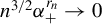 as
$n\rightarrow \infty $
 , then for any
$\tilde {w}$
 , as
$n\rightarrow \infty $
 ,

Moreover, if
$r_n$
 satisfies
$n^3\alpha _+^{r_n}\rightarrow 0$
 , then for any initial
$\tilde {w}$
 , as
$n\rightarrow \infty $
 ,

Theorem 10 establishes the asymptotic properties of the approximate MLE. It shows consistency in (i) based on Theorems 4 and 8, shows asymptotic normality based on Theorems 7 and 9 in (ii), and gives consistent estimates of the asymptotic covariance matrix based on the Hessian matrix and the outer product of scores in (iii) and (iv), respectively.
Theorem 10. (i) Assume Assumptions 1–4. If
$r_n$
 satisfies
$\alpha _+^{r_n}\rightarrow 0$
 as
$n\rightarrow \infty $
 , then for any initial
$\tilde {w}$
 , the approximate MLE
$\hat {\theta }^{(r_n)}_{n,\tilde {w}}\overset {p}{\rightarrow }\theta _0$
 ; (ii) Assume Assumptions 1–5 hold and that
$I(\theta _0)$
 is positive definite. If
$r_n$
 satisfies
$n^3\alpha _+^{r_n}\rightarrow 0$
 as
$n\rightarrow \infty $
 , then for any initial
$\tilde {w}$
 ,
$n^{1/2}(\hat {\theta }^{(r)}_{n,\tilde {w}}-\theta _0)\Rightarrow \mathbb {N}(0,I(\theta _0)^{-1})$
 ; (iii) Suppose that Assumptions 1–5 hold, and
$r_n$
 satisfies
$n^3\alpha _+^{r_n}\rightarrow 0$
 . For any
$\tilde {w}\in \mathbb {W}$
 ,
$n^{-1}\nabla _\theta ^2\overline {\ell }^{(r_n)}_{n,\tilde {w}}(\hat {\theta })\overset {p}{\rightarrow }I(\theta _0)$
 , if
$\hat {\theta }\overset {p}{\rightarrow }\theta _0$
 ; (iv) Suppose that Assumptions 1–5 hold, and
$r_n$
 satisfies
$n^2\alpha _+^{r_n}\rightarrow 0$
 . For any
$\tilde {w}\in \mathbb {W}$
 ,
$n^{-1}\sum _{t=1}^n\big (\nabla _\theta \log \overline {p}^{\hat {\theta }}_{r_n,\tilde {w}}(y_t|\mathbf {y}_1^{t-1})\nabla _\theta \log \overline {p}^{\hat {\theta }}_{r_n,\tilde {w}}(y_t|\mathbf {y}_1^{t-1})^T\big )\overset {p}{\rightarrow }I(\theta _0)$
 , if
$\hat {\theta }\overset {p}{\rightarrow }\theta _0$
 .
Remark 3. The condition
$n^3\alpha _+^{r_n}\to 0$
 required for the asymptotic normality in Theorem 10(ii) implies that
$r_n$
 must diverge as
$n\to \infty $
 , but the divergence can be relatively slow. In particular, since
$\alpha _+ \in (0,1)$
 , the condition
$n^3\alpha _+^{r_n}\to 0$
 is satisfied if
$r_n = C \log n$
 for some constant
$C> 3 / |\log (\alpha _+)|$
 . Hence, a logarithmic growth rate of
$r_n$
 is sufficient to guarantee the required condition, indicating that the increase of
$r_n$
 with the sample size can be relatively mild.Footnote
4
5 APPROXIMATION ERROR AND CHOICE OF r
This section provides practical guidelines for assessing the approximation error and selecting an appropriate value of r.
Section 4 shows that the approximation error is negligible if r increases with n to infinity. In practice, however, the magnitude of this error in finite samples remains unknown. We therefore propose a method to quantify this error. Although the exact likelihood and hence the true approximation error are computationally infeasible, the approximate likelihood can be computed for any given r. By comparing approximate likelihoods computed at successively larger values of r, we can bound the error. We express the error as

The next theorem characterizes
$|\overline {\ell }_{n,\tilde {w}}^{(\gamma )}(\theta )-\overline {\ell }_{n,\tilde {w}}^{(\gamma +1)}(\theta )|$
 on the right-hand side of (59).
Theorem 11. Assume Assumptions 1–4. Constant
$c>0$
 exists such that for any initialization
$w_0=\tilde {w}$
 , there exist constants
$c_m,c_N>0$
 and sequences of positive random variables
$m_t$
 and
$N_t$
 satisfying for all
$t\geq \gamma $
 ,
$\mathbb {E}_0\mathrm {sup}_{\theta \in \Theta }m_t^2<c_m$
 ,
$\mathbb {E}_0\mathrm {sup}_{\theta \in \Theta }N_t<c_N$
 , and for all
$\theta \in \Theta $
 ,

Theorem 11 implies that
$|\overline {\ell }_{n,\tilde {w}}^{(\gamma )}(\theta )-\overline {\ell }_{n,\tilde {w}}^{(\gamma +1)}(\theta )|$
 decreases exponentially in
$\gamma $
 . Let
$d(\gamma )\triangleq |\overline {\ell }_{n,\tilde {w}}^{(\gamma )}(\theta )-\overline {\ell }_{n,\tilde {w}}^{(\gamma +1)}(\theta )|$
 . Then, for some random variable
$K>0$
 and
$0<a<1$
 ,

In practice, we can choose
$\bar {r}\geq r$
 and estimate a conservative decay factor

The maximization starts from
$\gamma =2$
 because, in applications, one typically begins with small values of r and increases it sequentially. Using this conservative decay factor, the bound in (59) can be written as

Because Proposition 1 indicates that the approximation error grows with
$\alpha _{\max }(\theta )$
 , this procedure may be applied to the parameter value with a large
$\alpha _{\max }(\theta )$
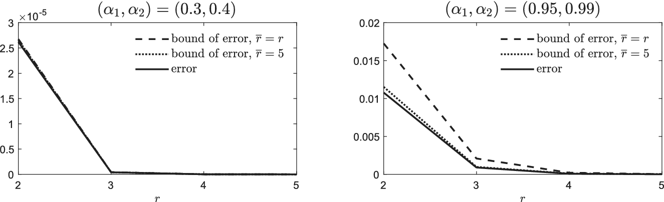
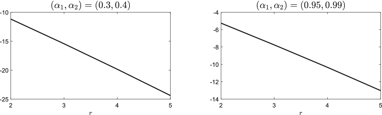
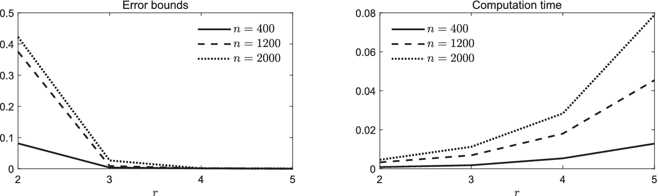
 to obtain a conservative error bound. As shown in the simulations in Section 7.2, a larger
$\overline {r}$
 yields a tighter upper bound. Then, in practice, choosing a smaller
$\overline {r}$
 reduces computational cost and typically leads to a more conservative upper bound, ensuring that the error bound is not underestimated.
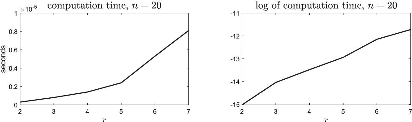
From Proposition 1, the approximation error decreases with r exponentially. Moreover, the computational cost increases exponentially with r, because the Kalman filter must be applied to each truncated regime path, with the total number of paths being
$J^r$
 , where J denotes the number of regimes. This trade-off supports the choice of a small r in practice. Practitioners may begin with small values, such as
$r=2,3,4$
 , compute the corresponding approximation errors and record the computation times, and then select an r that balances accuracy with available computational resources. If the error at
$r=4$
 still exceeds the desired tolerance, r can be increased further.
6 DISCUSSION ON THE CHOICE OF THE NUMBER OF REGIMES
The study is based on the premise that the number of regimes J has been correctly specified. In practice, however, J needs to be chosen from the data using statistical methods. The development of a rigorous inferential procedure for the number of regimes goes beyond the purpose of this article. In what follows, we discuss the main challenges and a possible starting point for future research.
Most methods for detecting the number of regimes rely on statistical tests. As shown in Qu and Zhuo (Reference Qu and Zhuo2021), the asymptotic null distribution of the likelihood ratio in MS models depends on which parameters are allowed to switch and on whether regressors are strictly or weakly exogenous. Thus, bootstrap methods can be inconsistent if they fail to reproduce the null covariance structure, and information criteria may fail because their penalties depend only on model dimension and cannot distinguish which parameters switch.
The challenge in testing the number of regimes is that some nuisance parameters are unidentified under the null hypothesis, and the score function is zero under the restricted MLE. Thus, the standard asymptotic analysis of the statistical test breaks down. Hansen (Reference Hansen1992) viewed the likelihood function as a stochastic process and obtained a bound for the asymptotic distribution of the likelihood ratio statistic. Cho and White (Reference Cho and White2007) isolated the unidentified parameters and took the supremum over them, thereby avoiding expansion with respect to them, and used higher-order expansions to address the zero-score problem. One limitation is that they replaced the recursive conditional regime probability with a constant mixture weight, thereby ignoring the serial correlation in the regime process. Qu and Zhuo (Reference Qu and Zhuo2021) addressed the limitation by explicitly modeling the stochastic conditional regime probability and deriving its derivatives, which allows them to conduct higher-order expansions in an MS setting. However, most existing results focus on testing one regime against two regimes. A general and readily applicable theory for testing J regimes against
$J+1$
 regimes remains limited.
Extending these results to MS state-space models requires additional work. The presence of a latent continuous state changes the likelihood expansion and the associated limiting distribution, so extending the existing MS results to the MS state-space setting would require rederiving the higher-order expansion and the corresponding limiting distribution. It is also necessary to characterize how the higher-order expansion of the approximate likelihood differs asymptotically from that of the exact likelihood. Moreover, although this study provides a method for choosing the truncation parameter r in maximum likelihood estimation, the choice of r requires separate analysis in the testing problem. We leave these issues for future research.
7 SIMULATION
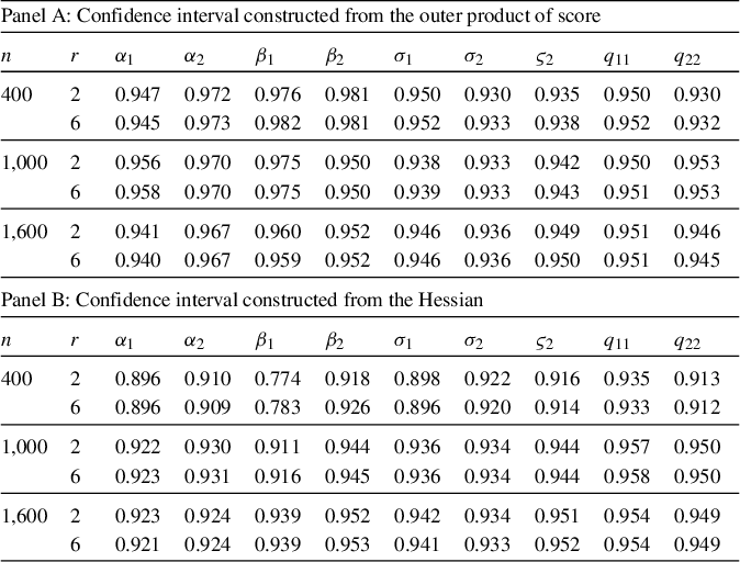
This section presents simulation experiments that illustrate the theoretical results and the practical performance of the approximation algorithm. Section 7.1 compares the log-likelihood functions obtained from the collapsing steps in (19) and (20). Section 7.2 examines the bias–complexity trade-off of the approximation algorithm and evaluates the proposed error-bounding method. Section 7.3 illustrates how to choose the truncation number r in practice. Section 7.4 compares the auxiliary particle filter and the Kalman–collapsing approximation algorithm. Section 7.5 examines how well the asymptotic distribution approximates the finite-sample distribution of the approximate MLE. Additional simulation results on approximation errors, Theorem 11, and regime persistence are reported in the Supplementary Material.
Unless otherwise stated, all simulations in this section use the following baseline data-generating process. Data are generated from (1) and (2) with
$J=2$
 and
$\theta _0=(\alpha _1,\alpha _2,\beta _1,\beta _2,\sigma _1,\sigma _2,\varsigma _1,\varsigma _2,q_{11},q_{22}) =(0.4,0.7,1,2,1,2,1,3,0.7,0.7)$
 . We use the initialization
$(\tilde x,\tilde s)=(0,1)$
 throughout.
7.1 Difference between Collapsing Methods
Section 7.1 examines the difference in the log-likelihood functions with the collapsing steps in (19) and (20). We generate 1,000 datasets from the baseline data-generating process for each of the two sample sizes,
$n=200$
 and
$n=2,000$
 . For each dataset, we compute the approximate log-likelihood function based on the simple collapsing (20)
$\overline {\ell }^{(r)}_{n,\tilde {w}}(\theta )$
 and that with Kim’s collapsing method (19)
$\overline {\ell }^{(r)\text {Kim}}_{n,\tilde {w}}(\theta )$
 with truncation number
$r=2, 4$
 .
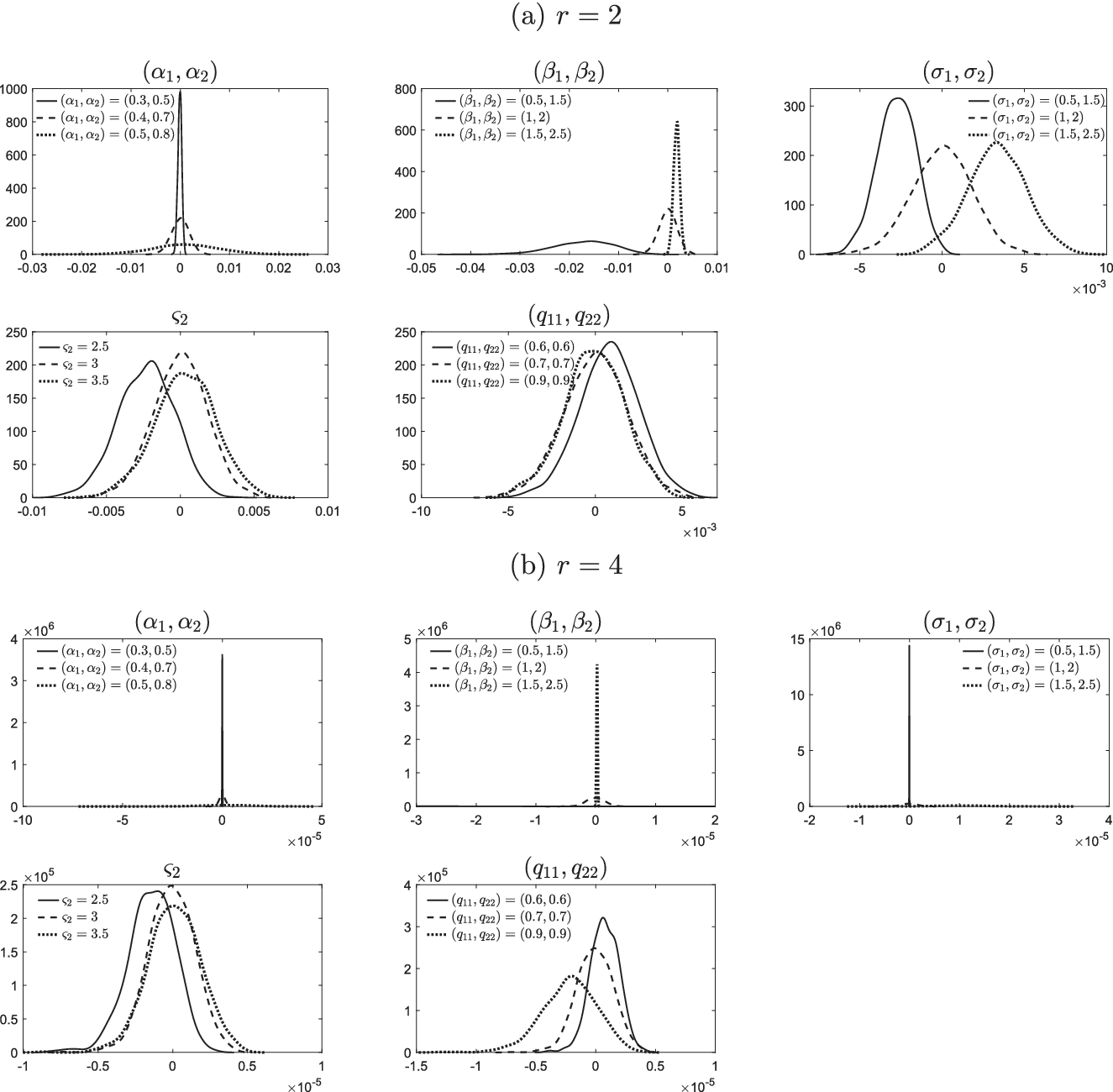
For
$n=2,000$
 , Figure 1 plots the kernel density estimates of
$\overline {\ell }^{(r)}_{n,\tilde {w}}(\theta )-\overline {\ell }^{(r)\text {Kim}}_{n,\tilde {w}}(\theta )$
 with parameters at the specified values and the other parameters at their true values. Figure 1 shows that
$|\overline {\ell }^{(r)}_{n,\tilde {w}}(\theta )-\overline {\ell }^{(r)\text {Kim}}_{n,\tilde {w}}(\theta )|$
 is generally no larger than 0.02 when
$r=2$
 and no larger than 0.0001 when
$r=4$
 . For reference, the averages of
$\overline {\ell }^{(r)}_{n,\tilde {w}}(\theta _0)$
 across 1,000 simulation experiments are
$-5,622.033$
 for both
$r=2$
 and
$r=4$
 . Thus, the difference in likelihood functions caused by different collapsing methods is small. The results of
$n=200$
 are presented in Figure B.1 in the Supplementary Material. The difference at
$n=200$
 is smaller than that for
$n=2,000$
 , indicating that the difference increases with n and decreases with r. The difference is also large when
$(\alpha _1,\alpha _2)$
 is large.
$\overline {\ell }^{(r)}_{n,\tilde {w}}(\theta )-\overline {\ell }^{(r)\text {Kim}}_{n,\tilde {w}}(\theta )$
 ,
$n=2,000$
 . Note: Each panel plots the kernel densities of
$\overline {\ell }^{(r)}_{n,\tilde {w}}(\theta )-\overline {\ell }^{(r)\text {Kim}}_{n,\tilde {w}}(\theta )$
 with one parameter at the specified value and the other parameters at their true values. For reference, the average of
$\overline {\ell }^{(r)}_{n,\tilde {w}}(\theta _0)$
 across 1,000 replications is
$-5,622.03$
 for both
$r=2$
 and
$r=4$
 .

Figure 1 Long description
The figure contains ten panels total, split into two groups of five.
Section a, r equals 2, contains five panels:
1. Top-left, alpha sub 1, alpha sub 2: Three curves centered at 0. The solid line is a sharp peak, while dashed and dotted lines are wider.
2. Top-center, beta sub 1, beta sub 2: Shows a broad distribution on the left and a very sharp, high peak near 0.002 on the right.
3. Top-right, sigma sub 1, sigma sub 2: Three distinct bell curves shifted along the x-axis, which is scaled by 10 super minus 3.
4. Bottom-left, zeta sub 2: Three overlapping bell curves centered near 0.
5. Bottom-center, q sub 1 1, q sub 2 2: Three overlapping bell curves centered near 0, with the x-axis scaled by 10 super minus 3.
Section b, r equals 4, contains five panels with similar parameter labels but different scales:
1. Top-left, alpha sub 1, alpha sub 2: A single extremely sharp vertical spike at 0, with the y-axis reaching 4 times 10 super 6 and x-axis scaled by 10 super minus 5.
2. Top-center, beta sub 1, beta sub 2: A sharp vertical spike at 0 reaching 5 times 10 super 6.
3. Top-right, sigma sub 1, sigma sub 2: A sharp vertical spike at 0 reaching 15 times 10 super 6.
4. Bottom-left, zeta sub 2: Three overlapping bell curves centered near 0, with the y-axis reaching 2.5 times 10 super 5.
5. Bottom-center, q sub 1 1, q sub 2 2: Three overlapping bell curves centered near 0, with the y-axis reaching 4 times 10 super 5 and x-axis scaled by 10 super minus 5.
7.2 Approximation Error, Computation Cost, and Error Bounding Method
This section examines the bias–complexity trade-off of the approximation algorithm and the performance of the error bounding method from Section 5.
We first examine how the approximation error and computation cost vary with r. Using a small sample size of
$n=20$
 , we compute the exact likelihood function, which becomes computationally infeasible for larger n. We generate 1,000 datasets from the baseline data-generating process with
$n=20$
 . For each dataset, we compute the approximation error for
$r = 2,\ldots ,5$
 at
$(\alpha _1,\alpha _2)=(0.3,0.4)$
 and
$(0.95,0.99)$
 , and record the computation time. Figures 2 and 3 plot the average approximation error and its logarithm across 1,000 replications. The logarithm of the error is linear in r, indicating that the approximation error decreases exponentially with r. Figure 4 plots the average computation time and its logarithm. The logarithm of computation time increases almost linearly with r, indicating that the computation time increases exponentially with r.
Approximation errors and error bounds,
$n=20$
 . Note: The figure displays the average approximation errors and the error bounds across 1,000 simulated datasets for
$n=20$
 . The left and right panels are evaluated at
$(\alpha _1,\alpha _2)=(0.3,0.4)$
 and
$(0.95,0.99)$
 , respectively. The other parameters are fixed at their true values.

Figure 2 Long description
Two panels show data for r on the x-axis ranging from 2 to 5.
Left panel: Titled (alpha sub 1, alpha sub 2) = (0.3, 0.4). The y-axis is scaled by 10 super minus 5, ranging from 0 to 3. Three lines (bound of error r-bar = r, bound of error r-bar = 5, and error) are nearly identical. They show a sharp linear decrease from approximately 2.6 at r = 2 to near zero at r = 3, remaining flat through r = 5.
Right panel: Titled (alpha sub 1, alpha sub 2) = (0.95, 0.99). The y-axis ranges from 0 to 0.02.
- The dashed line (bound of error r-bar = r) starts at 0.017 at r = 2, drops to 0.002 at r = 3, and reaches zero by r = 4.
- The dotted line (bound of error r-bar = 5) starts at 0.0115 at r = 2 and drops to 0.001 at r = 3.
- The solid line (error) starts lowest at 0.01 at r = 2 and converges with the dotted line at r = 3, both reaching zero by r = 4.
Log approximation error,
$n=20.$
 Note: The figure displays the average logarithm of approximation errors across 1,000 simulated datasets for
$n=20$
 . The left and right panels are evaluated at
$(\alpha _1,\alpha _2)=(0.3,0.4)$
 and
$(0.95,0.99)$
 , respectively. The other parameters are fixed at their true values.

Figure 3 Long description
The two panels share a common x-axis labeled r, ranging from 2 to 5. The y-axis represents the log approximation error.
* The left panel is titled (alpha sub 1, alpha sub 2) = (0.3, 0.4). The y-axis ranges from -25 to -10. A single solid black line shows a steep linear decrease, starting near -11 at r = 2 and ending near -24 at r = 5.
* The right panel is titled (alpha sub 1, alpha sub 2) = (0.95, 0.99). The y-axis ranges from -14 to -4. A single solid black line shows a linear decrease, starting near -5.5 at r = 2 and ending at -13 at r = 5.
Computation time and its logarithm,
$n=20$
 . Note: The figure displays the average computation time and its logarithm across 1,000 simulated datasets for
$n=20$
 and
$(\alpha _1,\alpha _2)=(0.3,0.4)$
 . The computation time for
$(\alpha _1,\alpha _2)=(0.95,0.99)$
 is almost identical and is omitted.

Figure 4 Long description
The image contains two panels arranged horizontally.
Left Panel: A line graph titled computation time, n equals 20. The y-axis is labeled seconds and scaled by 10 super minus 5, with tick marks from 0 to 1. The x-axis is labeled r and ranges from 2 to 7. The data shows a non-linear upward trend. The curve starts near 0 at r equals 2, rises slowly to approximately 0.24 at r equals 5, and then increases more steeply to approximately 0.8 at r equals 7.
Right Panel: A line graph titled log of computation time, n equals 20. The y-axis represents the logarithmic scale with tick marks from minus 15 to minus 11. The x-axis is labeled r and ranges from 2 to 7. The data shows a positive linear-like trend. The line starts at minus 15 for r equals 2, reaches approximately minus 14 at r equals 3, and continues a steady ascent to approximately minus 11.7 at r equals 7.
Next, we use the same simulated data to evaluate the method for bounding the approximation error. We consider two choices of
$\overline {r}$
 :
$\overline {r}=r$
 and
$\overline {r}=5$
 . Figure 2 plots average approximation errors and error bounds across the 1,000 datasets. The bounds with both
$\overline {r}=r$
 and
$\overline {r}=5$
 lie slightly above the errors, indicating that the bounding method performs well. Moreover,
$\overline {r}=5$
 provides a tighter upper bound.
7.3 Choice of r
We illustrate our procedure for selecting r. We simulate one dataset for each sample size
$n=400, 1,200, 2,000$
 under the baseline data-generating process, calculate the approximation error bounds, and record the computation time for
$r=2,\ldots ,5$
 and
$\overline {r}=r$
 and
$\overline {r}=5$
 . Figure 5 plots the computation time and the approximation error bounds evaluated at
$(\alpha _1,\alpha _2)=(0.95,0.99)$
 . Because the plots for
$\overline {r}=r$
 essentially overlap with those for
$\overline {r}=5$
 , we only plot the case of
$\overline {r}=r$
 . For reference, the log-likelihood values for
$r=2$
 when
$n=400,1,200$
 , and
$2,000$
 are
$-1,165.5$
 ,
$-3,592.5$
 , and
$-5,789.1$
 , respectively. If the maximum tolerable error for a practitioner is 0.1, one may choose
$r=2$
 for
$n=400$
 and
$r=3$
 for
$n=1,200$
 and 2,000, provided that the computation times shown in the right panel of Figure 5 are acceptable.
Approximation error bounds and computation time. Note: The left and right panels display the error bounds and computation time, respectively, for
$r=2,\ldots ,5$
 ,
$\overline {r}=r$
 , and
$n=400, 1,200, 2,000$
 . The error bounds are evaluated at
$(\alpha _1,\alpha _2)=(0.95,0.99)$
 and the remaining fixed at their true values.

Figure 5 Long description
The image consists of two side-by-side line graphs. Both graphs share a horizontal x-axis labeled r with integer values from 2 to 5. Each graph contains three lines representing different values of n: a solid line for n equals 400, a dashed line for n equals 1,200, and a dotted line for n equals 2,000.
* Left Panel: Titled Error bounds. The vertical y-axis ranges from 0 to 0.5. All three lines show a sharp non-linear decrease. At r equals 2, the error is highest, with the dotted line near 0.45 and the solid line near 0.1. By r equals 3, all lines drop significantly toward zero, remaining nearly flat and overlapping at the baseline for r values 4 and 5.
* Right Panel: Titled Computation time. The vertical y-axis ranges from 0 to 0.08. All three lines show a non-linear increase as r increases. The dotted line for n equals 2,000 shows the steepest upward trend, reaching approximately 0.07 at r equals 5. The dashed line for n equals 1,200 shows a moderate increase to approximately 0.045. The solid line for n equals 400 shows the slowest growth, ending near 0.015 at r equals 5.
7.4 Comparison of Kalman–Collapsing Approximation Algorithm and Auxiliary Particle Filter
This section uses simulation to compare the performance of the auxiliary particle filter and the Kalman–collapsing algorithm.
We generate 1,000 datasets, each of sample size
$n=20$
 using the baseline data-generating process. For this small sample size, exact likelihood functions remain computationally tractable. For each dataset, we compute: (i) approximation error
$|\overline {\ell }_{n,\tilde {w}}^{(r)}(\theta )-\ell _{n,\tilde {w}}(\theta )|$
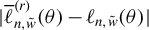 for
$r=2,\ldots ,5$
 and (ii) the auxiliary particle filter error
$|\ell _{n,\tilde {w}}^{\text {APF}}(\theta )-\ell _{n,\tilde {w}}(\theta )|$
 with particle size M and resample size R set to
$M=R=10{,}000, 50{,}000, 100{,}000$
 . All likelihood functions are evaluated at
$(\alpha _1,\alpha _2)=(0.3,0.4)$
 and
$(0.95,0.99)$
 , with the remaining parameters fixed at their true values. Computation times are also recorded for all methods.
For both algorithms, smaller errors are achieved at the cost of increased computation time. To facilitate comparison, Figure 6 plots the average log approximation errors against log computation times. The approximation algorithm reduces the error much faster as computation time increases than the auxiliary particle filter. Moreover, it achieves smaller errors with lower computation time than the auxiliary particle filter.
Log error and log computation time,
$n=20$
 . Note: This figure plots the log errors against the log computation time for the approximation algorithm with
$r=2,\ldots ,5$
 and the auxiliary particle filter (APF) with particle size M and resample size R set to
$M=R=10,000, 50,000$
 , and 100,000. Solid and dashed lines correspond to
$(\alpha _1,\alpha _2)=(0.95,0.99)$
 and (0.3,0.4), respectively. The other parameters are fixed at their true values.

Figure 6 Long description
The x-axis represents time in seconds on a log-scale ranging from minus 6 to 6. The y-axis represents absolute error on a log-scale ranging from minus 25 to 0.
Four distinct data series are plotted:
1. Approximation algorithm with alpha sub 1, alpha sub 2 equals 0.95, 0.99: Represented by a solid line with circular markers. It starts at the top-left at r equals 2 and descends diagonally to the right, ending at r equals 5 with an error of approximately minus 13.
2. Approximation algorithm with alpha sub 1, alpha sub 2 equals 0.3, 0.4: Represented by a dashed line with circular markers. It starts lower than the first series at r equals 2 and descends more steeply to the right, ending at r equals 5 with an error of approximately minus 24.
3. A P F error with alpha sub 1, alpha sub 2 equals 0.95, 0.99: Represented by a solid line with square markers located in the top-right quadrant. It shows a very slight downward slope as M increases from 10,000 to 100,000, maintaining a high error near minus 2.
4. A P F error with alpha sub 1, alpha sub 2 equals 0.3, 0.4: Represented by a dashed line with square markers located just below the previous A P F series. It also shows a slight downward slope as M increases, with error values between minus 3 and minus 4.
A legend in the bottom-right quadrant confirms these mappings, distinguishing between the approximation error and A P F error using solid and dashed lines for the different alpha parameter sets.
To assess how the two algorithms may perform when the sample size exceeds 20, Figure 7 displays the average errors at each time period,
$|\log \overline {p}_{r,\tilde {w}}^{\theta }(y_t|\mathbf {y}_1^{t-1})-\log p_{\tilde {w}}^{\theta }(y_t|\mathbf {y}_1^{t-1})|$
 and
$|\log p_{\tilde {w}}^{\theta ,\text {APF}}(y_t|\mathbf {y}_1^{t-1})-\log p_{\tilde {w}}^{\theta }(y_t|\mathbf {y}_1^{t-1})|$
 ,
$t=8,\ldots ,20$
 , across 1,000 replications. The approximation errors remain largely stable over time, consistent with Proposition 1. In contrast, the auxiliary particle filter errors exhibit an upward trend as t increases. If this pattern persists for larger sample sizes, the Kalman–collapsing algorithm is expected to outperform the auxiliary particle filter as n grows.
APF and approximation errors at each period,
$t=8,9,\ldots ,20$
 . Note: The upper panel plots the average of the approximation errors of the Kalman-collapsing filter
$|\log \overline {p}^{\theta }_{r,\tilde {w}}(y_t|\mathbf {y}_1^{t-1})-\log p^{\theta }_{\tilde {w}}(y_t|\mathbf {y}_1^{t-1})|$
 across 1,000 datasets for
$t = 8, 9, \ldots , 20$
 . The lower panel plots the average of the computation errors of the auxiliary particle filter
$|\log p^{\theta ,\text {APF}}_{\tilde {w}}(y_t|\mathbf {y}_1^{t-1})-\log p^{\theta }_{\tilde {w}}(y_t|\mathbf {y}_1^{t-1})|$
 across 1,000 datasets for
$t = 8, 9, \ldots , 20$
 with the resampling size M and the particle size R being 10,000, 50,000, and 100,000.

Figure 7 Long description
The image consists of four line graphs arranged in a two-by-two grid. All graphs share an x-axis representing time periods from 8 to 20.
Top-left panel: Titled times 10 super minus 6 approximation error with alpha sub 1, alpha sub 2 equals 0.3, 0.4. The y-axis ranges from 0 to 4. A solid line for r equals 2 fluctuates between 2.5 and 3.2. Dashed and dotted lines for r equals 3 and r equals 4 remain nearly flat at zero.
Top-right panel: Titled times 10 super minus 3 approximation error with alpha sub 1, alpha sub 2 equals 0.95, 0.99. The y-axis ranges from 0 to 2.5. The solid line for r equals 2 fluctuates between 1.4 and 1.9. The dashed line for r equals 3 is flat near 0.1, and the dotted line for r equals 4 is flat at zero.
Bottom-left panel: Titled A P F error with alpha sub 1, alpha sub 2 equals 0.3, 0.4. The y-axis ranges from 0 to 0.2. Three lines show an upward trend. The solid line for M equals R equals 10,000 rises from 0.09 to 0.15. The dashed line for M equals R equals 50,000 rises from 0.05 to 0.08. The dotted line for M equals R equals 100,000 rises from 0.03 to 0.06.
Bottom-right panel: Titled A P F error with alpha sub 1, alpha sub 2 equals 0.95, 0.99. The y-axis ranges from 0.1 to 0.6. All lines show a steady linear increase. The solid line for M equals R equals 10,000 rises from 0.2 to 0.38. The dashed line for M equals R equals 50,000 rises from 0.14 to 0.29. The dotted line for M equals R equals 100,000 rises from 0.13 to 0.26.
7.5 Finite-Sample Distribution of Approximate MLE
This section uses simulation to examine how well the asymptotic distribution approximates the distribution of the MLE in finite samples. We generate 1,000 datasets from the baseline data-generating process for
$n=400$
 ,
$1,000$
 , and
$1,600$
 . For each dataset, we estimate the approximate MLE with
$r=2, 6$
 . Using Theorem 10, we construct the confidence intervals from the Hessian matrix and the outer product of the score. Table 1 reports the frequency at which the 95% confidence interval contains the true parameter.Footnote
5
Coverage frequency of the asymptotic 95% confidence intervals

Table 1 Long description
The table is divided into two sections. Panel A: Confidence interval constructed from the outer product of score. Panel B: Confidence interval constructed from the Hessian. Both panels share the same column headers: n, r, alpha sub 1, alpha sub 2, beta sub 1, beta sub 2, sigma sub 1, sigma sub 2, varsigma sub 2, q sub 1 1, and q sub 2 2.
In Panel A, for n = 400 and r = 2, values range from 0.930 to 0.981. For n = 1,000 and r = 2, values range from 0.933 to 0.975. For n = 1,600 and r = 2, values range from 0.936 to 0.967. Increasing r to 6 shows minimal variation in coverage frequency.
In Panel B, for n = 400 and r = 2, values show more variance, particularly for beta sub 1 at 0.774, while others range between 0.896 and 0.935. As n increases to 1,600, the coverage frequencies stabilize closer to the 0.95 target, with values ranging from 0.921 to 0.954.
The coverage frequencies in Panel A are closer to 95% than the ones in Panel B, especially for
$n=400$
 . The confidence intervals constructed from the outer product of score outperform those constructed from the Hessian matrix in small samples. The coverage frequencies with
$r=2$
 and
$r=6$
 are close. This might be because the approximate likelihood functions for
$r=2$
 and
$r=6$
 are close for this experiment. To further verify it, we compute
$|\hat {\theta }_n^{(6)}-\hat {\theta }_n^{(2)}|$
 for each replication and report the median in Table 2.
Median of
$|\hat {\theta }_n^{(6)}-\hat {\theta }_n^{(2)}|$


Table 2 Long description
The table consists of 10 columns and 4 rows including the header.
Header row labels from left to right: n, alpha sub 1, alpha sub 2, beta sub 1, beta sub 2, sigma sub 1, sigma sub 2, varsigma sub 2, q sub 11, and q sub 22.
Row 1: n is 400. Values are 0.0004, 0.0002, 0.0008, 0.0013, 0.0011, 0.0038, 0.0029, 0.00003, and 0.00003.
Row 2: n is 1,000. Values are 0.0002, 0.0001, 0.0006, 0.0010, 0.0007, 0.0028, 0.0013, 0.00002, and 0.00002.
Row 3: n is 1,600. Values are 0.0002, 0.0001, 0.0004, 0.0006, 0.0004, 0.0016, 0.0007, 0.00001, and 0.00001.
As n increases, the values for all parameters generally decrease.
Table 2 shows that
$\hat {\theta }_n^{(6)}$
 and
$\hat {\theta }_n^{(2)}$
 are close. Moreover, given that the coverage frequencies in Panel A for
$r=2$
 are mostly close to 95%, the estimator with
$r=2$
 and the confidence intervals constructed from the outer product of scores perform well in finite samples. Further increases in r do not lead to noticeable improvements for the sample sizes typically used in practice. These finite-sample findings are consistent with the theoretical requirement in Theorem 10, where asymptotic normality is established under the condition
$n^3\alpha _+^{r_n}\to 0$
 . This condition permits
$r_n$
 to diverge at a relatively slow rate and is satisfied, for example, by
$r_n=C\log n$
 with
$C> 3/|\log \alpha _+|$
 . Hence, a small value such as
$r=2$
 suffices in practice, which corroborates the good simulation results reported above.Footnote
6
8 CONCLUSION AND DISCUSSION
This study provides the first theoretical analysis of the approximation algorithm for MS state-space models. We derive upper bounds for the approximation errors in likelihood computation and latent variable inference, showing that they decay exponentially with the truncation length r at the rate of
$\alpha _{\max }(\theta )^{r-1}$
 . We prove that the approximate MLE is consistent and asymptotically normal, provided that r increases with the sample size at an appropriate rate. In addition, we propose a practical method for bounding the approximation error by comparing approximate likelihoods computed at successively larger values of r, which provides guidance for choosing r by balancing approximation accuracy and computational complexity. The results offer both theoretical justification and practical guidance for applying the approximation algorithm in empirical work.
SUPPLEMENTARY MATERIAL
The supplementary material for this article can be found at https://doi.org/10.1017/S0266466626100723.
COMPETING INTEREST STATEMENT
The author declares that no competing interests exist.
FUNDING STATEMENT
This work was supported by the National Natural Science Foundation of China (NSFC) under Grant Number 72303068.