1 Introduction
When the density of a stably stratified fluid is a function of two scalar fields with differing diffusivities, and one of these scalars is unstably stratified, there exists the potential for a double-diffusive instability to evolve (Radko Reference Radko2013). A prominent example concerns the ocean, as heat diffuses one hundred times faster in water than salt. Even if the two scalars diffuse at identical rates, an instability can form if the unstably stratified scalar has a settling velocity associated with it (Alsinan, Meiburg & Garaud Reference Alsinan, Meiburg and Garaud2017; Reali et al. Reference Reali, Garaud, Alsinan and Meiburg2017). This situation can be encountered in buoyant river outflows, where sediment is unstably stratified while the overall density gradient is stable due to salinity (Burns & Meiburg Reference Burns and Meiburg2012, Reference Burns and Meiburg2015; Yu, Hsu & Balachandar Reference Yu, Hsu and Balachandar2013, Reference Yu, Hsu and Balachandar2014).
An important feature of river outflows is the presence of shear along the lower boundary of the river plume. The effect of this shear on the growth of double-diffusive fingering has been the subject of several studies (Linden Reference Linden1974; Smyth & Kimura Reference Smyth and Kimura2007, Reference Smyth and Kimura2011; Radko et al. Reference Radko, Ball, Colosi and Flanagan2015), which found it to dampen the growth of instability modes with wavenumber aligned in the direction of the shear, thereby resulting in the formation of salt sheets. In studying the influence of asymptotically weak Couette flow on double-diffusive fingering, Linden (Reference Linden1974) found that for large Prandtl numbers shear had a damping influence. For small Prandtl numbers, on the other hand, shear may amplify the fingering instability. Smyth & Kimura (Reference Smyth and Kimura2007, Reference Smyth and Kimura2011) employed hyperbolic tangent temperature, salinity and velocity profiles within a linear stability analysis as well as direct numerical simulations (DNS) to analyse the effect of shear on fingering. These authors examined fluxes, the dissipation ratio and growth rates, and arrived at the conclusion that shear dampens the fingering instability. Radko et al. (Reference Radko, Ball, Colosi and Flanagan2015) showed that in a DNS, fingering fluxes in the presence of shear are a factor of 2–3 times smaller than without shear. Here we will investigate the mechanisms of the effects of finite-strength shear on both the double-diffusive and the settling-driven instability. Towards this end, we would like to employ an infinite domain to eliminate the effects of solid boundaries, as well as shear profiles that avoid the presence of competing shear instabilities. As we will see, all of these goals can be accomplished by means of a transient growth analysis, which has the added benefit of providing detailed insight into the physical mechanisms at work.
Section 2 will define the problem and derive the linearized equations describing the instability growth. In § 3, we describe the adjoint method employed for calculating the objective gradients for the optimization procedure. Section 4 presents the results of this analysis, along with their physical interpretation.
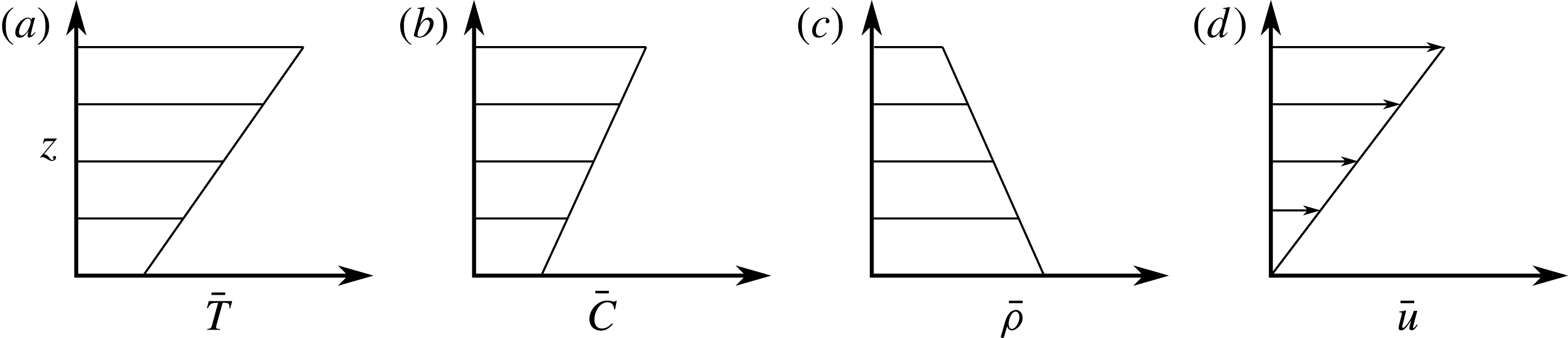
Background temperature
 $\bar{T}$
, particle concentration
 $\bar{C}$
, density
 $\bar{\unicode[STIX]{x1D70C}}$
and
 $x$
-velocity
 $\bar{u}$
. Within the stable overall density stratification, the particle concentration is unstably stratified.

2 Problem formulation
Before presenting the details of our approach, we first provide a quick overview and justification for it. Several strategies may appear feasible for investigating the effect of shear on double-diffusive and settling-driven instabilities. Linden (Reference Linden1974) performed a linear stability analysis for a vertically bounded Couette flow with linear temperature and salinity gradients, as sketched in figure 1. However, in trying to extend this approach to the settling-driven instability, we found the eigenvalues and eigenvectors to strongly depend on the size of the domain, and to be dominated by boundary effects. This difficulty cannot be eliminated by considering a sedimenting particle concentration field in an unbounded error function-type background shear instead, as this set-up violates the quasi-steady base state approximation. For these reasons, we opt to solve an optimization problem in order to identify the maximum perturbation growth within a linearized framework. This approach no longer requires a quasi-steady state approximation, and it allows us to consider a wave-like perturbation with a time-dependent slope in an unbounded Couette flow. This concept is known as Kelvin waves, and it has been successfully employed in the study of the planar Couette flow (Kelvin Reference Kelvin1887; Rosen Reference Rosen1971; Knobloch Reference Knobloch1984; Shepherd Reference Shepherd1985; Craik & Criminale Reference Craik and Criminale1986).
Consider the Navier–Stokes equations in the Boussinesq approximation, along with convection–diffusion transport equations for temperature
 $T^{\ast }$
and particle concentration
 $C^{\ast }$
, a linear equation of state for the fluid density and the continuity equation. With asterisks denoting dimensional quantities, these read
 $$\begin{eqnarray}\displaystyle & \displaystyle {\displaystyle \frac{\unicode[STIX]{x2202}\boldsymbol{u}^{\ast }}{\unicode[STIX]{x2202}t^{\ast }}}+\boldsymbol{u}^{\ast }\boldsymbol{\cdot }\unicode[STIX]{x1D735}^{\ast }\boldsymbol{u}^{\ast }=-{\displaystyle \frac{1}{\unicode[STIX]{x1D70C}_{0}^{\ast }}}\unicode[STIX]{x1D735}^{\ast }P^{\ast }+\unicode[STIX]{x1D708}^{\ast }\unicode[STIX]{x1D6FB}^{\ast 2}\boldsymbol{u}^{\ast }+{\displaystyle \frac{\unicode[STIX]{x1D70C}^{\ast }}{\unicode[STIX]{x1D70C}_{0}^{\ast }}}\boldsymbol{g}^{\ast }, & \displaystyle\end{eqnarray}$$
 $$\begin{eqnarray}\displaystyle & \displaystyle {\displaystyle \frac{\unicode[STIX]{x2202}T^{\ast }}{\unicode[STIX]{x2202}t^{\ast }}}+\boldsymbol{u}^{\ast }\boldsymbol{\cdot }\unicode[STIX]{x1D735}^{\ast }T^{\ast }=k_{T}^{\ast }\unicode[STIX]{x1D6FB}^{\ast 2}T^{\ast }, & \displaystyle\end{eqnarray}$$
 $$\begin{eqnarray}\displaystyle & \displaystyle {\displaystyle \frac{\unicode[STIX]{x2202}C^{\ast }}{\unicode[STIX]{x2202}t^{\ast }}}+\boldsymbol{u}^{\ast }\boldsymbol{\cdot }\unicode[STIX]{x1D735}^{\ast }C^{\ast }=k_{C}^{\ast }\unicode[STIX]{x1D6FB}^{\ast 2}C^{\ast }+V_{st}^{\ast }{\displaystyle \frac{\unicode[STIX]{x2202}C^{\ast }}{\unicode[STIX]{x2202}z^{\ast }}}, & \displaystyle\end{eqnarray}$$
 $$\begin{eqnarray}\displaystyle & \displaystyle \unicode[STIX]{x1D70C}^{\ast }=\unicode[STIX]{x1D70C}_{0}^{\ast }(1-\unicode[STIX]{x1D6FC}^{\ast }(T^{\ast }-T_{0}^{\ast })+\unicode[STIX]{x1D6FD}^{\ast }(C^{\ast }-C_{0}^{\ast })), & \displaystyle\end{eqnarray}$$
 $$\begin{eqnarray}\displaystyle & \displaystyle \unicode[STIX]{x1D735}^{\ast }\boldsymbol{\cdot }\boldsymbol{u}^{\ast }=0. & \displaystyle\end{eqnarray}$$
Here
 $\boldsymbol{u}^{\ast }=(u^{\ast },v^{\ast },w^{\ast })$
represents the velocity,
 $\unicode[STIX]{x1D70C}^{\ast }$
indicates the density,
 $\unicode[STIX]{x1D70C}_{0}^{\ast }$
is the density of a reference state with
 $T^{\ast }=T_{0}^{\ast }$
and
 $C^{\ast }=C_{0}^{\ast }$
,
 $P^{\ast }$
denotes the pressure,
 $\boldsymbol{g}^{\ast }=(0,0,-g^{\ast })$
the gravity vector,
 $\unicode[STIX]{x1D708}^{\ast }$
the kinematic viscosity,
 $k_{T}^{\ast }$
and
 $k_{C}^{\ast }$
represent the diffusivity of heat and particles and
 $\unicode[STIX]{x1D6FC}^{\ast }$
and
 $\unicode[STIX]{x1D6FD}^{\ast }$
express the density dependence on temperature and particle concentration.
 $V_{st}^{\ast }$
is the Stokes settling velocity
 $$\begin{eqnarray}\displaystyle & \displaystyle V_{st}^{\ast }={\displaystyle \frac{2g^{\ast }r_{p}^{\ast 2}(\unicode[STIX]{x1D70C}_{p}^{\ast }-\unicode[STIX]{x1D70C}_{0}^{\ast })}{9\unicode[STIX]{x1D707}^{\ast }}}, & \displaystyle\end{eqnarray}$$
where
 $r_{p}^{\ast }$
denotes the particle radius,
 $\unicode[STIX]{x1D70C}_{p}^{\ast }$
the particle density and
 $\unicode[STIX]{x1D707}^{\ast }$
the dynamic viscosity. Each variable
 $q^{\ast }$
can be thought of as the sum of a background or base state
 $\bar{q}^{\ast }$
, and the perturbation
 ${q^{\ast }}^{\prime }$
from that state. We assume a background state of the form
 $$\begin{eqnarray}\displaystyle & \displaystyle \bar{\boldsymbol{u}}^{\ast }=(S^{\ast }z^{\ast },0,0), & \displaystyle\end{eqnarray}$$
 $$\begin{eqnarray}\displaystyle & \displaystyle \bar{T}^{\ast }=\bar{T}_{z}^{\ast }z^{\ast }, & \displaystyle\end{eqnarray}$$
 $$\begin{eqnarray}\displaystyle & \displaystyle \bar{C}^{\ast }=\bar{C}_{z}^{\ast }(z^{\ast }+V_{st}^{\ast }t^{\ast }), & \displaystyle\end{eqnarray}$$
 $$\begin{eqnarray}\displaystyle & \displaystyle {\displaystyle \frac{\unicode[STIX]{x2202}\bar{P}^{\ast }}{\unicode[STIX]{x2202}z^{\ast }}}=-\unicode[STIX]{x1D70C}_{0}^{\ast }g^{\ast }\left[1-\unicode[STIX]{x1D6FC}^{\ast }(\bar{T}^{\ast }-T_{0}^{\ast })+\unicode[STIX]{x1D6FD}^{\ast }(\bar{C}^{\ast }-C_{0}^{\ast })\right], & \displaystyle\end{eqnarray}$$
where
 $\bar{T}_{z}^{\ast }$
and
 $\bar{C}_{z}^{\ast }$
are positive constants, as sketched in figure 1. We remark that at a given location, the background particle concentration increases uniformly with time as a result of particle settling acting on the uniform background particle concentration
 $z$
-gradient. The density contributions due to the background profiles, as well as the reference temperature and particle concentration, can be absorbed into the background pressure
 $\bar{P}^{\ast }$
. By substituting
 $q^{\ast }=\bar{q}^{\ast }+{q^{\ast }}^{\prime }$
into the governing equations, we obtain
 $$\begin{eqnarray}\displaystyle & \displaystyle {\displaystyle \frac{\text{D}{u^{\ast }}^{\prime }}{\text{D}t^{\ast }}}+S^{\ast }z^{\ast }{\displaystyle \frac{\unicode[STIX]{x2202}{u^{\ast }}^{\prime }}{\unicode[STIX]{x2202}x^{\ast }}}+{w^{\ast }}^{\prime }S^{\ast }=-{\displaystyle \frac{1}{\unicode[STIX]{x1D70C}_{0}^{\ast }}}{\displaystyle \frac{\unicode[STIX]{x2202}{P^{\ast }}^{\prime }}{\unicode[STIX]{x2202}x^{\ast }}}+\unicode[STIX]{x1D708}^{\ast }\unicode[STIX]{x1D6FB}^{\ast 2}{u^{\ast }}^{\prime }, & \displaystyle\end{eqnarray}$$
 $$\begin{eqnarray}\displaystyle & \displaystyle {\displaystyle \frac{\text{D}{v^{\ast }}^{\prime }}{\text{D}t^{\ast }}}+S^{\ast }z^{\ast }{\displaystyle \frac{\unicode[STIX]{x2202}{v^{\ast }}^{\prime }}{\unicode[STIX]{x2202}x^{\ast }}}=-{\displaystyle \frac{1}{\unicode[STIX]{x1D70C}_{0}^{\ast }}}{\displaystyle \frac{\unicode[STIX]{x2202}{P^{\ast }}^{\prime }}{\unicode[STIX]{x2202}y^{\ast }}}+\unicode[STIX]{x1D708}^{\ast }\unicode[STIX]{x1D6FB}^{\ast 2}{v^{\ast }}^{\prime }, & \displaystyle\end{eqnarray}$$
 $$\begin{eqnarray}\displaystyle & \displaystyle {\displaystyle \frac{\text{D}{w^{\ast }}^{\prime }}{\text{D}t^{\ast }}}+S^{\ast }z^{\ast }{\displaystyle \frac{\unicode[STIX]{x2202}{w^{\ast }}^{\prime }}{\unicode[STIX]{x2202}x^{\ast }}}=-{\displaystyle \frac{1}{\unicode[STIX]{x1D70C}_{0}^{\ast }}}{\displaystyle \frac{\unicode[STIX]{x2202}{P^{\ast }}^{\prime }}{\unicode[STIX]{x2202}z^{\ast }}}+\unicode[STIX]{x1D708}^{\ast }\unicode[STIX]{x1D6FB}^{\ast 2}{w^{\ast }}^{\prime }+g^{\ast }(\unicode[STIX]{x1D6FC}^{\ast }{T^{\ast }}^{\prime }-\unicode[STIX]{x1D6FD}^{\ast }{C^{\ast }}^{\prime }), & \displaystyle\end{eqnarray}$$
 $$\begin{eqnarray}\displaystyle & \displaystyle {\displaystyle \frac{\text{D}{T^{\ast }}^{\prime }}{\text{D}t^{\ast }}}+S^{\ast }z^{\ast }{\displaystyle \frac{\unicode[STIX]{x2202}{T^{\ast }}^{\prime }}{\unicode[STIX]{x2202}x^{\ast }}}=k_{T}^{\ast }\unicode[STIX]{x1D6FB}^{\ast 2}{T^{\ast }}^{\prime }-{w^{\ast }}^{\prime }{\displaystyle \frac{\unicode[STIX]{x2202}\bar{T}^{\ast }}{\unicode[STIX]{x2202}z^{\ast }}}, & \displaystyle\end{eqnarray}$$
 $$\begin{eqnarray}\displaystyle & \displaystyle {\displaystyle \frac{\text{D}{C^{\ast }}^{\prime }}{\text{D}t^{\ast }}}+S^{\ast }z^{\ast }{\displaystyle \frac{\unicode[STIX]{x2202}{C^{\ast }}^{\prime }}{\unicode[STIX]{x2202}x^{\ast }}}=k_{C}^{\ast }\unicode[STIX]{x1D6FB}^{\ast 2}{C^{\ast }}^{\prime }-{w^{\ast }}^{\prime }{\displaystyle \frac{\unicode[STIX]{x2202}\bar{C}^{\ast }}{\unicode[STIX]{x2202}z^{\ast }}}+V_{st}^{\ast }{\displaystyle \frac{\unicode[STIX]{x2202}{C^{\ast }}^{\prime }}{\unicode[STIX]{x2202}z^{\ast }}}, & \displaystyle\end{eqnarray}$$
 $$\begin{eqnarray}\displaystyle & \displaystyle \unicode[STIX]{x1D735}^{\ast }\boldsymbol{\cdot }{\boldsymbol{u}^{\ast }}^{\prime }=0, & \displaystyle\end{eqnarray}$$
where
 $\text{D}/\text{D}t^{\ast }=\unicode[STIX]{x2202}/\unicode[STIX]{x2202}t^{\ast }+\boldsymbol{u}^{\ast }\boldsymbol{\cdot }\unicode[STIX]{x1D735}^{\ast }$
denotes the material derivative. We non-dimensionalize the problem using the length, time, temperature and concentration scales according to Radko (Reference Radko2013), where we replace salinity with particle concentration
 $$\begin{eqnarray}\displaystyle & \displaystyle d_{c}^{\ast }=\left({\displaystyle \frac{k_{T}^{\ast }\unicode[STIX]{x1D708}^{\ast }}{g^{\ast }\unicode[STIX]{x1D6FC}^{\ast }|\bar{T}_{z}^{\ast }|}}\right)^{1/4},\quad t_{c}^{\ast }={\displaystyle \frac{(d_{c}^{\ast })^{2}}{k_{T}^{\ast }}},\quad u_{c}^{\ast }={\displaystyle \frac{k_{T}^{\ast }}{d_{c}^{\ast }}},\quad P_{c}^{\ast }={\displaystyle \frac{\unicode[STIX]{x1D70C}_{0}^{\ast }\unicode[STIX]{x1D708}^{\ast }k_{T}^{\ast }}{(d_{c}^{\ast })^{2}}},\qquad \quad & \displaystyle\end{eqnarray}$$
 $$\begin{eqnarray}\displaystyle & \displaystyle T_{c}^{\ast }=d_{c}^{\ast }|\bar{T}_{z}^{\ast }|,\quad C_{c}^{\ast }={\displaystyle \frac{\unicode[STIX]{x1D6FC}^{\ast }}{\unicode[STIX]{x1D6FD}^{\ast }}}T_{c}^{\ast }. & \displaystyle\end{eqnarray}$$
Representative oceanic values of
 $\unicode[STIX]{x1D708}^{\ast }=10^{-6}~\text{m}~\text{s}^{-2}$
,
 $k_{T}^{\ast }=\unicode[STIX]{x1D708}^{\ast }/7$
,
 $|\bar{T}_{z}^{\ast }|=0.01~\text{K}~\text{m}^{-1}$
and
 $\unicode[STIX]{x1D6FC}^{\ast }=2.07\times 10^{-4}~\text{K}^{-1}$
yield
 $d_{c}^{\ast }\approx 1~\text{cm}$
and
 $t_{c}^{\ast }\approx 10^{3}~\text{s}$
. After applying these scales and dropping the primes, we obtain the non-dimensional governing equations
 $$\begin{eqnarray}\displaystyle & \displaystyle {\displaystyle \frac{\unicode[STIX]{x2202}u}{\unicode[STIX]{x2202}t}}+Sz{\displaystyle \frac{\unicode[STIX]{x2202}u}{\unicode[STIX]{x2202}x}}+wS+\boldsymbol{u}\boldsymbol{\cdot }\unicode[STIX]{x1D735}u=-Pr{\displaystyle \frac{\unicode[STIX]{x2202}P}{\unicode[STIX]{x2202}x}}+Pr\unicode[STIX]{x1D6FB}^{2}u, & \displaystyle\end{eqnarray}$$
 $$\begin{eqnarray}\displaystyle & \displaystyle {\displaystyle \frac{\unicode[STIX]{x2202}v}{\unicode[STIX]{x2202}t}}+Sz{\displaystyle \frac{\unicode[STIX]{x2202}v}{\unicode[STIX]{x2202}x}}+\boldsymbol{u}\boldsymbol{\cdot }\unicode[STIX]{x1D735}v=-Pr{\displaystyle \frac{\unicode[STIX]{x2202}P}{\unicode[STIX]{x2202}y}}+Pr\unicode[STIX]{x1D6FB}^{2}v, & \displaystyle\end{eqnarray}$$
 $$\begin{eqnarray}\displaystyle & \displaystyle {\displaystyle \frac{\unicode[STIX]{x2202}w}{\unicode[STIX]{x2202}t}}+Sz{\displaystyle \frac{\unicode[STIX]{x2202}w}{\unicode[STIX]{x2202}x}}+\boldsymbol{u}\boldsymbol{\cdot }\unicode[STIX]{x1D735}w=-Pr{\displaystyle \frac{\unicode[STIX]{x2202}P}{\unicode[STIX]{x2202}z}}+Pr\unicode[STIX]{x1D6FB}^{2}w+Pr(T-C), & \displaystyle\end{eqnarray}$$
 $$\begin{eqnarray}\displaystyle & \displaystyle {\displaystyle \frac{\unicode[STIX]{x2202}T}{\unicode[STIX]{x2202}t}}+Sz{\displaystyle \frac{\unicode[STIX]{x2202}T}{\unicode[STIX]{x2202}x}}+w+\boldsymbol{u}\boldsymbol{\cdot }\unicode[STIX]{x1D735}T=\unicode[STIX]{x1D6FB}^{2}T, & \displaystyle\end{eqnarray}$$
 $$\begin{eqnarray}\displaystyle & \displaystyle {\displaystyle \frac{\unicode[STIX]{x2202}C}{\unicode[STIX]{x2202}t}}+Sz{\displaystyle \frac{\unicode[STIX]{x2202}C}{\unicode[STIX]{x2202}x}}+{\displaystyle \frac{w}{R_{\unicode[STIX]{x1D70C}}}}+\boldsymbol{u}\boldsymbol{\cdot }\unicode[STIX]{x1D735}C={\displaystyle \frac{1}{\unicode[STIX]{x1D70F}}}\unicode[STIX]{x1D6FB}^{2}C+V_{p}{\displaystyle \frac{\unicode[STIX]{x2202}C}{\unicode[STIX]{x2202}z}}, & \displaystyle\end{eqnarray}$$
 $$\begin{eqnarray}\displaystyle & \displaystyle \unicode[STIX]{x1D735}\boldsymbol{\cdot }\boldsymbol{u}=0. & \displaystyle\end{eqnarray}$$
Dimensionless parameters arise in the form
 $$\begin{eqnarray}\displaystyle & \displaystyle Pr={\displaystyle \frac{\unicode[STIX]{x1D708}^{\ast }}{k_{T}^{\ast }}},\quad \unicode[STIX]{x1D70F}={\displaystyle \frac{k_{T}^{\ast }}{k_{C}^{\ast }}},\quad V_{p}={\displaystyle \frac{V_{st}^{\ast }}{u_{c}^{\ast }}},\quad R_{\unicode[STIX]{x1D70C}}={\displaystyle \frac{\unicode[STIX]{x1D6FC}^{\ast }\bar{T}_{z}^{\ast }}{\unicode[STIX]{x1D6FD}^{\ast }\bar{C}_{z}^{\ast }}}, & \displaystyle\end{eqnarray}$$
where
 $Pr$
is the Prandtl number. Linearization around the background state, and using the continuity equation to eliminate pressure results in
 $$\begin{eqnarray}\displaystyle & \displaystyle {\displaystyle \frac{\unicode[STIX]{x2202}}{\unicode[STIX]{x2202}t}}(\unicode[STIX]{x1D6FB}^{2}w)=-Sz{\displaystyle \frac{\unicode[STIX]{x2202}}{\unicode[STIX]{x2202}x}}\unicode[STIX]{x1D6FB}^{2}w+Pr\unicode[STIX]{x1D6FB}^{4}w+Pr\left({\displaystyle \frac{\unicode[STIX]{x2202}^{2}T}{\unicode[STIX]{x2202}x^{2}}}+{\displaystyle \frac{\unicode[STIX]{x2202}^{2}T}{\unicode[STIX]{x2202}y^{2}}}\right)-Pr\left({\displaystyle \frac{\unicode[STIX]{x2202}^{2}C}{\unicode[STIX]{x2202}x^{2}}}+{\displaystyle \frac{\unicode[STIX]{x2202}^{2}C}{\unicode[STIX]{x2202}y^{2}}}\right),\quad & \displaystyle\end{eqnarray}$$
 $$\begin{eqnarray}\displaystyle & \displaystyle {\displaystyle \frac{\unicode[STIX]{x2202}T}{\unicode[STIX]{x2202}t}}=-Sz{\displaystyle \frac{\unicode[STIX]{x2202}T}{\unicode[STIX]{x2202}x}}-w+\unicode[STIX]{x1D6FB}^{2}T, & \displaystyle\end{eqnarray}$$
 $$\begin{eqnarray}\displaystyle & \displaystyle {\displaystyle \frac{\unicode[STIX]{x2202}C}{\unicode[STIX]{x2202}t}}=-Sz{\displaystyle \frac{\unicode[STIX]{x2202}C}{\unicode[STIX]{x2202}x}}-{\displaystyle \frac{w}{R_{\unicode[STIX]{x1D70C}}}}+{\displaystyle \frac{1}{\unicode[STIX]{x1D70F}}}\unicode[STIX]{x1D6FB}^{2}C+V_{p}{\displaystyle \frac{\unicode[STIX]{x2202}C}{\unicode[STIX]{x2202}z}}. & \displaystyle\end{eqnarray}$$
We would like to eliminate the terms with explicit dependence on
 $z$
, so that we can transform the equations to wave space and assume an infinite domain for the perturbation fields. Toward this end, we assume that the solution has the form of a plane wave with time-varying wavenumbers
 $$\begin{eqnarray}\displaystyle & \displaystyle q(x,y,z,t)=\widetilde{q}(t)\exp [\text{i}k(t)x+\text{i}l(t)y+\text{i}m(t)z]. & \displaystyle\end{eqnarray}$$
Substitution into (2.26)–(2.28) yields
 $$\begin{eqnarray}\displaystyle {\displaystyle \frac{\text{d}}{\text{d}t}}(K^{2}\widetilde{w})+K^{2}\widetilde{w}\left(\text{i}{\displaystyle \frac{\text{d}k}{\text{d}t}}x+\text{i}{\displaystyle \frac{\text{d}l}{\text{d}t}}y+\text{i}{\displaystyle \frac{\text{d}m}{\text{d}t}}z\right) & = & \displaystyle -\text{i}kSzK^{2}\widetilde{w}-PrK^{4}\widetilde{w}\nonumber\\ \displaystyle & & \displaystyle +\,Pr(k^{2}+l^{2})(\widetilde{T}-\widetilde{C}),\end{eqnarray}$$
 $$\begin{eqnarray}\displaystyle {\displaystyle \frac{\text{d}\widetilde{T}}{\text{d}t}}+\widetilde{T}\left(\text{i}{\displaystyle \frac{\text{d}k}{\text{d}t}}x+\text{i}{\displaystyle \frac{\text{d}l}{\text{d}t}}y+\text{i}{\displaystyle \frac{\text{d}m}{\text{d}t}}z\right) & = & \displaystyle -\text{i}kSz\widetilde{T}-\widetilde{w}-K^{2}\widetilde{T},\end{eqnarray}$$
 $$\begin{eqnarray}\displaystyle {\displaystyle \frac{\text{d}\widetilde{C}}{\text{d}t}}+\widetilde{C}\left(\text{i}{\displaystyle \frac{\text{d}k}{\text{d}t}}x+\text{i}{\displaystyle \frac{\text{d}l}{\text{d}t}}y+\text{i}{\displaystyle \frac{\text{d}m}{\text{d}t}}z\right) & = & \displaystyle -\text{i}kSz\widetilde{C}-{\displaystyle \frac{\widetilde{w}}{R_{\unicode[STIX]{x1D70C}}}}-{\displaystyle \frac{1}{\unicode[STIX]{x1D70F}}}K^{2}\widetilde{C}\nonumber\\ \displaystyle & & \displaystyle +\,\text{i}mV_{p}\widetilde{C},\end{eqnarray}$$
where
 $$\begin{eqnarray}\displaystyle & \displaystyle K^{2}(t)=k(t)^{2}+l(t)^{2}+m(t)^{2}. & \displaystyle\end{eqnarray}$$
We now eliminate the explicit dependence on
 $z$
by strategically choosing
 $$\begin{eqnarray}\displaystyle {\displaystyle \frac{\text{d}k}{\text{d}t}}=0,\quad {\displaystyle \frac{\text{d}l}{\text{d}t}}=0,\quad {\displaystyle \frac{\text{d}m}{\text{d}t}}=-Sk. & & \displaystyle\end{eqnarray}$$
Substitution into (2.30)–(2.32) and rearranging into matrix form yields
 $$\begin{eqnarray}\displaystyle {\displaystyle \frac{\text{d}}{\text{d}t}}\left(\begin{array}{@{}c@{}}K^{2}\widetilde{w}\\ \widetilde{T}\\ \widetilde{C}\end{array}\right)=\left(\begin{array}{@{}ccc@{}}-PrK^{2} & Pr(k^{2}+l^{2}) & -Pr(k^{2}+l^{2})\\ -K^{-2} & -K^{2} & 0\\ -R_{\unicode[STIX]{x1D70C}}^{-1}K^{-2} & 0 & -\unicode[STIX]{x1D70F}^{-1}K^{2}+\text{i}(m_{0}-Skt)V_{p}\end{array}\right)\left(\begin{array}{@{}c@{}}K^{2}\widetilde{w}\\ \widetilde{T}\\ \widetilde{C}\end{array}\right)\quad & & \displaystyle\end{eqnarray}$$
now with
 $$\begin{eqnarray}\displaystyle & \displaystyle K^{2}(t)=k^{2}+l^{2}+(m_{0}-Skt)^{2}, & \displaystyle\end{eqnarray}$$
where
 $m_{0}$
denotes the initial value of
 $m(t)$
. Our objective is to characterize the effect of shear on the instability modes identified in Alsinan et al. (Reference Alsinan, Meiburg and Garaud2017), which are wave-like in the vertical direction, with time-invariant
 $m$
. In the present formulation of the sheared problem, the value of
 $m$
and the associated instantaneous growth rate varies in time. In order to reduce the parameter space for the following study, we will seek the optimal initial wave vector
 $(k,l,m_{0})$
that leads to largest growth over a finite time horizon
 $t_{\text{end}}$
for any given set of flow parameters. We keep in mind that the growth may not be exponential in time, and that the spatial shape of the mode is time dependent. The entire analysis can then be performed in wave space. For added convenience later on, we rewrite (2.35) as
 $$\begin{eqnarray}\displaystyle {\displaystyle \frac{\text{d}}{\text{d}t}}\left(\begin{array}{@{}c@{}}\widetilde{w}\\ \widetilde{T}\\ \widetilde{C}\end{array}\right)=\left(\begin{array}{@{}ccc@{}}\unicode[STIX]{x1D713}(t) & PrK^{-2}(k^{2}+l^{2}) & -PrK^{-2}(k^{2}+l^{2})\\ -1 & -K^{2} & 0\\ -R_{\unicode[STIX]{x1D70C}}^{-1} & 0 & -\unicode[STIX]{x1D70F}^{-1}K^{2}+\text{i}(m_{0}-Skt)V_{p}\end{array}\right)\left(\begin{array}{@{}c@{}}\widetilde{w}\\ \widetilde{T}\\ \widetilde{C}\end{array}\right), & & \displaystyle\end{eqnarray}$$
where the notation
 $$\begin{eqnarray}\displaystyle & \displaystyle \unicode[STIX]{x1D713}(t)=-PrK^{2}+2Sk(m_{0}-Skt)K^{-2} & \displaystyle\end{eqnarray}$$
is employed to save space.
Knobloch (Reference Knobloch1984) proved that Kelvin wave perturbations in unbounded stratified Couette flow are unconditionally stable, regardless of the shear rate
 $S$
. However, a strong velocity gradient in a finite-width stratified shear layer will typically lead to instability of the Kelvin–Helmholtz type. A sufficient criterion for stability of a stratified flow with respect to shear mechanisms, according to Howard (Reference Howard1961), Drazin & Reid (Reference Drazin and Reid1981), is that the gradient Richardson number is larger than
 $1/4$
. With the present definitions, this criterion is written as
 $$\begin{eqnarray}\displaystyle & \displaystyle Ri=-{\displaystyle \frac{g^{\ast }\overline{\unicode[STIX]{x1D70C}}_{z}^{\ast }}{\unicode[STIX]{x1D70C}_{0}\overline{u}_{z}^{\ast 2}}}=Pr{\displaystyle \frac{1-R_{\unicode[STIX]{x1D70C}}^{-1}}{S^{2}}}>{\displaystyle \frac{1}{4}}. & \displaystyle\end{eqnarray}$$
The objective of this study is to characterize how shear modifies the instabilities that are driven by diffusion and particle settling. While we choose unbounded Couette flow for our investigation, in order to exclude effects of vertical base flow inhomogeneity, we wish to stay in a parameter regime where shear-driven instability does not occur, even outside this special flow case. Parameter values
 $Pr\geqslant 0.2$
and
 $R_{\unicode[STIX]{x1D70C}}\geqslant 1.6$
will be considered in the following. A constant value
 $S=0.1$
of the shear parameter is chosen such that the criterion (2.39) is always satisfied.
3 Optimization procedure
We aim to identify the maximum of the gain
 $$\begin{eqnarray}\displaystyle & \displaystyle G={\displaystyle \frac{(|\widetilde{w}|^{2}+|\widetilde{T}|^{2}+|\widetilde{C}|^{2})|_{t=t_{\text{end}}}}{(|\widetilde{w}|^{2}+|\widetilde{T}|^{2}+|\widetilde{C}|^{2})|_{t=0}}} & \displaystyle\end{eqnarray}$$
with respect to
 $k$
,
 $l$
,
 $m_{0}$
and the complex initial conditions for
 $\widetilde{w}$
,
 $\widetilde{T}$
and
 $\widetilde{C}$
. In the absence of shear (
 $S=0$
), the equations depend only on
 $k^{2}+l^{2}$
instead of on
 $k$
and
 $l$
independently, so that we can set
 $l=0$
without loss of generality. When shear is present, its influence is removed if
 $k=0$
so that the unsheared result is recovered, although now as a function of
 $l$
instead of
 $k$
. In a linear stability analysis, growth rates for sheared double-diffusive fingering are generally lower for
 $k>0$
than for
 $k=0$
(Linden Reference Linden1974; Smyth & Kimura Reference Smyth and Kimura2007), so that we expect the formation of ‘salt sheets’ aligned in the direction of the shear, with
 $k=0$
. In the present investigation we set
 $l=0$
, so that we can isolate the effect of shear. We note that any problem with
 $l>0$
can be converted to one with
 $l=0$
, although with different
 $S$
- and
 $k$
-values, by the transformation
 $$\begin{eqnarray}\displaystyle & \displaystyle k\leftarrow \sqrt{k^{2}+l^{2}}, & \displaystyle\end{eqnarray}$$
 $$\begin{eqnarray}\displaystyle & \displaystyle S\leftarrow {\displaystyle \frac{Sk}{\sqrt{k^{2}+l^{2}}}}. & \displaystyle\end{eqnarray}$$
In anticipation of the findings to be discussed below, we remark that this transformation implies the following: if for
 $l=0$
, i.e. in the absence of spanwise perturbations, shear is observed to dampen the growth, we can conclude that the maximum sheared growth will likely occur for spanwise modes with
 $l>0$
and
 $k=0$
, for which the unsheared growth results are recovered.
Since the ordinary differential equation (ODE) for which we optimize is linear, multiplying the initial condition by a complex constant will not affect the gain in (3.1). To remove this degree of freedom, we set
 $$\begin{eqnarray}\displaystyle & \displaystyle (|\widetilde{w}|^{2}+|\widetilde{T}|^{2}+|\widetilde{C}|^{2})|_{t=0}=1 & \displaystyle\end{eqnarray}$$
and optimize for
 $$\begin{eqnarray}\displaystyle & \displaystyle G=(|\widetilde{w}|^{2}+|\widetilde{T}|^{2}+|\widetilde{C}|^{2})|_{t=t_{\text{end}}}. & \displaystyle\end{eqnarray}$$
We parameterize the initial condition constraint (3.4) by setting
 $$\begin{eqnarray}\displaystyle & \displaystyle \widetilde{w}_{t=0}=r_{w}\text{e}^{\text{i}\unicode[STIX]{x1D703}_{w}}, & \displaystyle\end{eqnarray}$$
 $$\begin{eqnarray}\displaystyle & \displaystyle \widetilde{T}_{t=0}=r_{T}\text{e}^{\text{i}\unicode[STIX]{x1D703}_{T}}, & \displaystyle\end{eqnarray}$$
 $$\begin{eqnarray}\displaystyle & \displaystyle \widetilde{C}_{t=0}=r_{C}\text{e}^{\text{i}\unicode[STIX]{x1D703}_{C}}. & \displaystyle\end{eqnarray}$$
Note that these three values can be multiplied by a factor of
 $\text{e}^{\text{i}\unicode[STIX]{x1D703}}$
for any
 $\unicode[STIX]{x1D703}$
without affecting (3.4). Consequently we set
 $$\begin{eqnarray}\displaystyle & \displaystyle \unicode[STIX]{x1D703}_{w}=0 & \displaystyle\end{eqnarray}$$
and only optimize for
 $\unicode[STIX]{x1D703}_{T}$
and
 $\unicode[STIX]{x1D703}_{C}$
. Equation (3.4) yields
 $$\begin{eqnarray}\displaystyle & \displaystyle r_{w}^{2}+r_{T}^{2}+r_{C}^{2}=1. & \displaystyle\end{eqnarray}$$
These three parameters and one constraint can be reduced to two free parameters
 $\unicode[STIX]{x1D719}_{1}$
and
 $\unicode[STIX]{x1D719}_{2}$
by using spherical coordinates
 $$\begin{eqnarray}\displaystyle & \displaystyle r_{w}=\cos (\unicode[STIX]{x1D719}_{1})\cos (\unicode[STIX]{x1D719}_{2}), & \displaystyle\end{eqnarray}$$
 $$\begin{eqnarray}\displaystyle & \displaystyle r_{T}=\sin (\unicode[STIX]{x1D719}_{1})\cos (\unicode[STIX]{x1D719}_{2}), & \displaystyle\end{eqnarray}$$
 $$\begin{eqnarray}\displaystyle & \displaystyle r_{C}=\sin (\unicode[STIX]{x1D719}_{2}). & \displaystyle\end{eqnarray}$$
To summarize, we need to optimize over the four initial condition variables
 $\unicode[STIX]{x1D703}_{T}$
,
 $\unicode[STIX]{x1D703}_{C}$
,
 $\unicode[STIX]{x1D719}_{1}$
and
 $\unicode[STIX]{x1D719}_{2}$
, from which the initial condition can be reconstructed by
 $$\begin{eqnarray}\displaystyle & \displaystyle \widetilde{w}=\cos (\unicode[STIX]{x1D719}_{1})\cos (\unicode[STIX]{x1D719}_{2}), & \displaystyle\end{eqnarray}$$
 $$\begin{eqnarray}\displaystyle & \displaystyle \widetilde{T}=\sin (\unicode[STIX]{x1D719}_{1})\cos (\unicode[STIX]{x1D719}_{2})\text{e}^{\text{i}\unicode[STIX]{x1D703}_{T}}, & \displaystyle\end{eqnarray}$$
 $$\begin{eqnarray}\displaystyle & \displaystyle \widetilde{C}=\sin (\unicode[STIX]{x1D719}_{2})\text{e}^{\text{i}\unicode[STIX]{x1D703}_{C}}. & \displaystyle\end{eqnarray}$$
With
 $l=0$
as discussed above, our goal is now to find the total derivative of
 $G$
with respect to
 $$\begin{eqnarray}\displaystyle \boldsymbol{p}=\left(\begin{array}{@{}c@{}}\unicode[STIX]{x1D719}_{1}\\ \unicode[STIX]{x1D719}_{2}\\ \unicode[STIX]{x1D703}_{T}\\ \unicode[STIX]{x1D703}_{C}\\ k\\ m_{0}\end{array}\right) & & \displaystyle\end{eqnarray}$$
and then employ its gradient in a gradient-based optimization algorithm such as Broyden–Fletcher–Goldfarb–Shanno (BFGS) or nonlinear conjugate gradient, which is available in Matlab through the fminunc() function. The default tolerance criterion is used, requiring that the infinity norm of the cost function gradient falls below
 $10^{-6}$
.
We calculate the gradient using the adjoint method, adapted from Gunzburger (Reference Gunzburger2000) and described in the following. The adjoint method allows us to calculate the gradient with a computational cost roughly equivalent to two evaluations of
 $G$
, as opposed to the finite difference method, which would require
 $O(n)$
evaluations, were
 $n$
is the length of
 $\boldsymbol{p}$
. We begin by defining a Lagrangian functional
 $L$
 $$\begin{eqnarray}\displaystyle L=G+\int _{0}^{t_{\text{end}}}(\boldsymbol{q}^{+})^{T}\left({\displaystyle \frac{\text{d}\boldsymbol{q}}{\text{d}t}}-A(t)\boldsymbol{q}\right)\text{d}t, & & \displaystyle\end{eqnarray}$$
where
 $\boldsymbol{q}^{+}$
is the Lagrange multiplier. We define
 $$\begin{eqnarray}\displaystyle A(t)=\left(\begin{array}{@{}cc@{}}\text{Re}(B(t)) & -\text{Im}(B(t))\\ \text{Im}(B(t)) & \text{Re}(B(t))\end{array}\right) & & \displaystyle\end{eqnarray}$$
with
 $$\begin{eqnarray}\displaystyle B(t)=\left(\begin{array}{@{}ccc@{}}-PrK^{2}+2Sk(m_{0}-Skt)K^{-2} & PrK^{-2}(k^{2}+l^{2}) & -PrK^{-2}(k^{2}+l^{2})\\ -1 & -K^{2} & 0\\ -R_{\unicode[STIX]{x1D70C}}^{-1} & 0 & -\unicode[STIX]{x1D70F}^{-1}K^{2}+\text{i}(m_{0}-Skt)V_{p}\end{array}\right) & & \displaystyle \nonumber\\ \displaystyle & & \displaystyle\end{eqnarray}$$
according to the system of ODEs in (2.37). The vector
 $\boldsymbol{q}$
and its initial condition
 $\boldsymbol{q}(0)$
are defined as
 $$\begin{eqnarray}\displaystyle \boldsymbol{q}(t)=\left(\begin{array}{@{}c@{}}\text{Re}(\widetilde{w}(t))\\ \text{Re}(\widetilde{T}(t))\\ \text{Re}(\widetilde{C}(t))\\ \text{Im}(\widetilde{w}(t))\\ \text{Im}(\widetilde{T}(t))\\ \text{Im}(\widetilde{C}(t))\end{array}\right),\quad \boldsymbol{q}(0)=\left(\begin{array}{@{}c@{}}\cos (\unicode[STIX]{x1D719}_{1})\cos (\unicode[STIX]{x1D719}_{2})\\ \sin (\unicode[STIX]{x1D719}_{1})\cos (\unicode[STIX]{x1D719}_{2})\cos (\unicode[STIX]{x1D703}_{T})\\ \sin (\unicode[STIX]{x1D719}_{2})\cos (\unicode[STIX]{x1D703}_{C})\\ 0\\ \sin (\unicode[STIX]{x1D719}_{1})\cos (\unicode[STIX]{x1D719}_{2})\sin (\unicode[STIX]{x1D703}_{T})\\ \sin (\unicode[STIX]{x1D719}_{2})\sin (\unicode[STIX]{x1D703}_{C})\end{array}\right). & & \displaystyle\end{eqnarray}$$
In (3.18), the Lagrange multiplier
 $\boldsymbol{q}^{+}$
can be chosen freely because we always enforce
 $$\begin{eqnarray}\displaystyle {\displaystyle \frac{\text{d}\boldsymbol{q}}{\text{d}t}}-A(t)\boldsymbol{q}=0. & & \displaystyle\end{eqnarray}$$
Because constraint (3.22) is always satisfied, we have
 $$\begin{eqnarray}\displaystyle {\displaystyle \frac{\text{d}L}{\text{d}\boldsymbol{p}}}={\displaystyle \frac{\text{d}G}{\text{d}\boldsymbol{p}}}. & & \displaystyle\end{eqnarray}$$
Our goal now is to find this gradient
 $\text{d}L/\text{d}\boldsymbol{p}$
in such a way that we will not have to calculate
 $\text{d}\boldsymbol{q}/\text{d}\boldsymbol{p}$
, except at
 $t=0$
, which is easily done using (3.21). Since
 $G$
has no explicit dependence on
 $\boldsymbol{p}$
,
 $\unicode[STIX]{x2202}G/\unicode[STIX]{x2202}\boldsymbol{p}=0$
, and we may begin with
 $$\begin{eqnarray}\displaystyle & \displaystyle {\displaystyle \frac{\text{d}L}{\text{d}\boldsymbol{p}}}={\displaystyle \frac{\unicode[STIX]{x2202}G}{\unicode[STIX]{x2202}\boldsymbol{q}(t_{\text{end}})}}{\displaystyle \frac{\text{d}\boldsymbol{q}(t_{\text{end}})}{\text{d}\boldsymbol{p}}}+\int _{0}^{t_{\text{end}}}(\boldsymbol{q}^{+})^{T}\left({\displaystyle \frac{\text{d}}{\text{d}\boldsymbol{p}}}{\displaystyle \frac{\text{d}\boldsymbol{q}}{\text{d}t}}-A(t){\displaystyle \frac{\text{d}\boldsymbol{q}}{\text{d}\boldsymbol{p}}}-{\displaystyle \frac{\text{d}A(t)}{\text{d}\boldsymbol{p}}}\boldsymbol{q}\right)\text{d}t & \displaystyle\end{eqnarray}$$
and use integration by parts on the term containing
 $\text{d}\boldsymbol{q}/\text{d}t$
 $$\begin{eqnarray}\displaystyle & \displaystyle \int _{0}^{t_{\text{end}}}(\boldsymbol{q}^{+})^{T}{\displaystyle \frac{\text{d}}{\text{d}\boldsymbol{p}}}{\displaystyle \frac{\text{d}\boldsymbol{q}}{\text{d}t}}\,\text{d}t=\left.\left((\boldsymbol{q}^{+})^{T}{\displaystyle \frac{\text{d}\boldsymbol{q}}{\text{d}\boldsymbol{p}}}\right)\right|_{t=t_{\text{end}}}-\left.\left((\boldsymbol{q}^{+})^{T}{\displaystyle \frac{\text{d}\boldsymbol{q}}{\text{d}\boldsymbol{p}}}\right)\right|_{t=0}-\int _{0}^{t_{\text{end}}}\left({\displaystyle \frac{\text{d}\boldsymbol{q}^{+}}{\text{d}t}}\right)^{T}{\displaystyle \frac{\text{d}\boldsymbol{q}}{\text{d}\boldsymbol{p}}}\,\text{d}t. & \displaystyle \nonumber\\ \displaystyle & & \displaystyle\end{eqnarray}$$
We substitute (3.25) into (3.24)
 $$\begin{eqnarray}\displaystyle {\displaystyle \frac{\text{d}L}{\text{d}\boldsymbol{p}}} & = & \displaystyle -\boldsymbol{q}^{+}(0)^{T}{\displaystyle \frac{\text{d}\boldsymbol{q}(0)}{\text{d}\boldsymbol{p}}}-\int _{0}^{t_{\text{end}}}(\boldsymbol{q}^{+})^{T}{\displaystyle \frac{\text{d}A(t)}{\text{d}\boldsymbol{p}}}\boldsymbol{q}\,\text{d}t\nonumber\\ \displaystyle & & \displaystyle \quad -\,\int _{0}^{t_{\text{end}}}\left(\left({\displaystyle \frac{\text{d}\boldsymbol{q}^{+}}{\text{d}t}}\right)^{T}+(\boldsymbol{q}^{+})^{T}A(t)\right){\displaystyle \frac{\text{d}\boldsymbol{q}}{\text{d}\boldsymbol{p}}}\,\text{d}t\nonumber\\ \displaystyle & & \displaystyle \quad +\left.\left[\left((\boldsymbol{q}^{+})^{T}+{\displaystyle \frac{\unicode[STIX]{x2202}G}{\unicode[STIX]{x2202}\boldsymbol{q}}}\right){\displaystyle \frac{\text{d}\boldsymbol{q}}{\text{d}\boldsymbol{p}}}\right]\right|_{t_{\text{end}}}\end{eqnarray}$$
and pick
 $\boldsymbol{q}^{+}$
so that there is only dependence on
 $\text{d}\boldsymbol{q}/\text{d}\boldsymbol{p}$
at
 $t=0$
. Noting that
 $G=\boldsymbol{q}(t_{\text{end}})^{T}\boldsymbol{q}(t_{\text{end}})$
, this yields
 $$\begin{eqnarray}\displaystyle \boldsymbol{q}^{+}(t_{\text{end}})=-\left({\displaystyle \frac{\unicode[STIX]{x2202}G}{\unicode[STIX]{x2202}\boldsymbol{q}(t_{\text{end}})}}\right)^{T}=-2\boldsymbol{q}(t_{\text{end}}), & & \displaystyle\end{eqnarray}$$
as well as an ODE for
 $\boldsymbol{q}^{+}$
 $$\begin{eqnarray}\displaystyle & \displaystyle {\displaystyle \frac{\text{d}\boldsymbol{q}^{+}}{\text{d}t}}=-A(t)^{T}\boldsymbol{q}^{+}, & \displaystyle\end{eqnarray}$$
which we integrate from
 $t=t_{\text{end}}$
to
 $t=0$
. This yields the gradient
 $$\begin{eqnarray}\displaystyle {\displaystyle \frac{\text{d}G}{\text{d}\boldsymbol{p}}}=-\boldsymbol{q}^{+}(0)^{T}{\displaystyle \frac{\text{d}\boldsymbol{q}(0)}{\text{d}\boldsymbol{p}}}-\int _{0}^{t_{\text{end}}}(\boldsymbol{q}^{+})^{T}{\displaystyle \frac{\text{d}A(t)}{\text{d}\boldsymbol{p}}}\boldsymbol{q}\,\text{d}t. & & \displaystyle\end{eqnarray}$$
The method used to calculate the gradient is now as follows. For a given initial condition
 $\boldsymbol{q}(0)$
,
 $k$
and
 $m_{0}$
, we integrate (3.22) in time from
 $t=0$
to
 $t=t_{\text{end}}$
. We then use the result
 $\boldsymbol{q}(t_{\text{end}})$
to calculate
 $\boldsymbol{q}^{+}(t_{\text{end}})$
using (3.27). With
 $\boldsymbol{q}^{+}(t_{\text{end}})$
as an initial condition, we integrate (3.28) from
 $t=t_{\text{end}}$
to
 $t=0$
. We then use
 $\boldsymbol{q}(t)$
,
 $\boldsymbol{q}^{+}(t)$
and
 $\boldsymbol{q}(0)$
along with (3.21) to evaluate (3.29).
4 Results
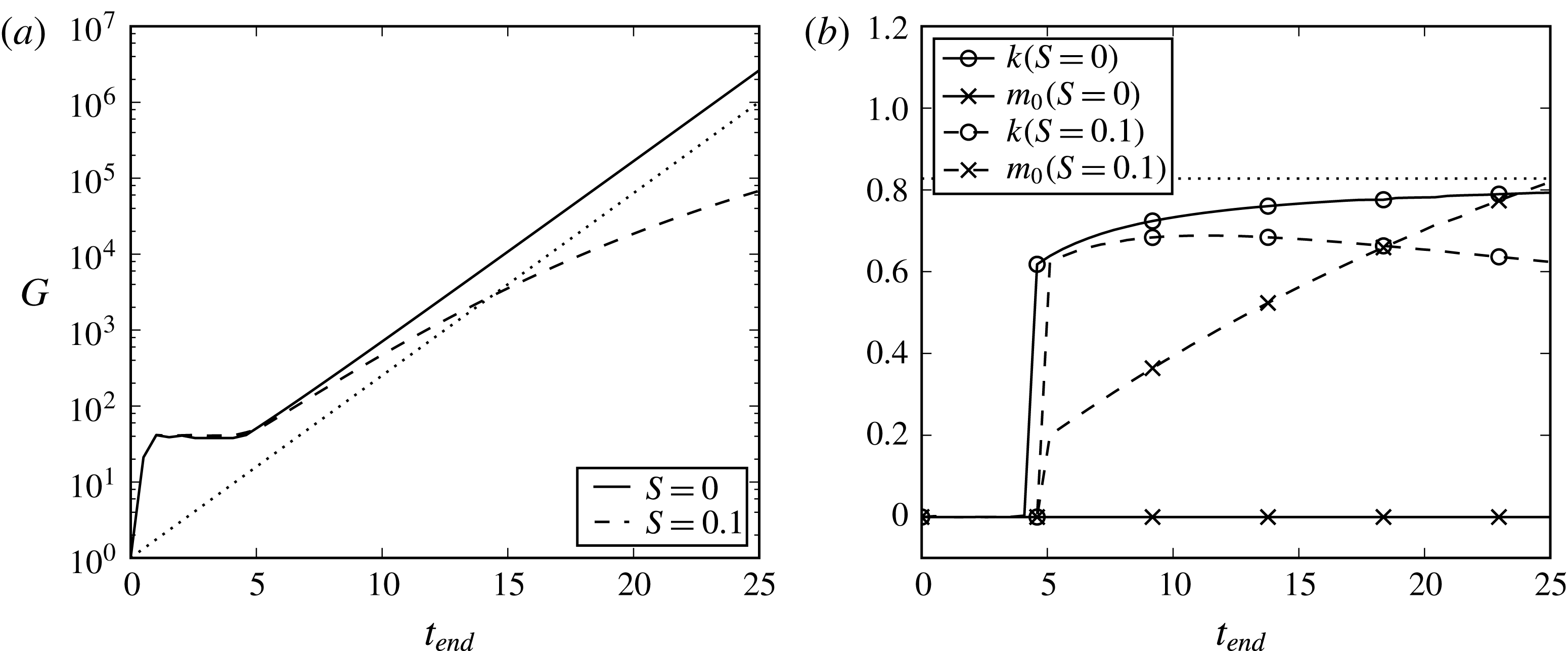
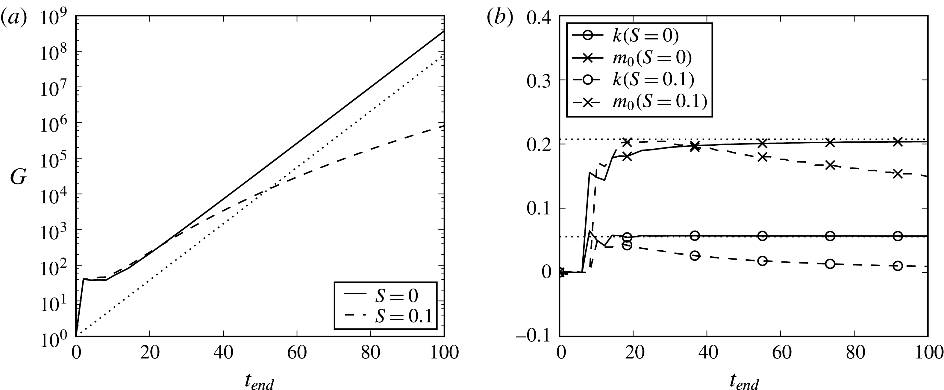
Figure 2 shows a representative set of optimization results for the fingering instability, with
 $Pr=7$
,
 $\unicode[STIX]{x1D70F}=100$
,
 $R_{\unicode[STIX]{x1D70C}}=2$
and
 $V_{p}=0$
. It compares the case
 $S=0.1$
with its no-shear counterpart. For the no-shear case, the dotted lines demonstrate the excellent agreement between the optimization results for large
 $t_{\text{end}}$
and corresponding linear stability results. For small times
 $t_{\text{end}}\leqslant 5$
, on the other hand, the optimization results deviate strongly from the linear stability results. In the following, we will first examine the reasons for this transient phenomenon in more detail, and then proceed to discuss the effects of
 $Pr$
,
 $\unicode[STIX]{x1D70F}$
,
 $R_{\unicode[STIX]{x1D70C}}$
and
 $V_{p}$
on the fingering- and settling-driven instabilities in the presence of shear.
Optimized gain
 $G$
and corresponding
 $k$
and
 $m_{0}$
as a function of the time interval
 $[0,t_{\text{end}}]$
for the fingering instability. The other parameters are
 $Pr=7$
,
 $\unicode[STIX]{x1D70F}=100$
,
 $R_{\unicode[STIX]{x1D70C}}=2$
and
 $V_{p}=0$
. The dotted lines correspond to linear stability results for the maximum growth rate and corresponding
 $k$
-value, in the absence of shear.

4.1 Initial growth and the Orr mechanism
The initial fast growth seen in figure 2 occurs when
 $k\rightarrow 0$
and
 $m_{0}\rightarrow 0$
. It is present with and without shear, and as we will see below, it also exists for the settling-driven instability, cf. figure 8. In this limit, the system of ODEs (2.37) reduces to
 $$\begin{eqnarray}\displaystyle {\displaystyle \frac{\unicode[STIX]{x2202}}{\unicode[STIX]{x2202}t}}\left(\begin{array}{@{}c@{}}\widetilde{w}\\ \widetilde{T}\\ \widetilde{C}\end{array}\right)=\left(\begin{array}{@{}ccc@{}}0 & Pr & -Pr\\ -1 & 0 & 0\\ -R_{\unicode[STIX]{x1D70C}}^{-1} & 0 & 0\end{array}\right)\left(\begin{array}{@{}c@{}}\widetilde{w}\\ \widetilde{T}\\ \widetilde{C}\end{array}\right), & & \displaystyle\end{eqnarray}$$
so that
 $S$
no longer appears. The fast initial growth occurs when
 $\widetilde{T}$
and
 $\widetilde{C}$
initially have opposite signs, so they act in phase on the density field, as higher
 $\widetilde{T}$
and lower
 $\widetilde{C}$
both reduce the overall density. As a result
 $\widetilde{w}$
grows strongly, which in turn will cause
 $\widetilde{T}$
and
 $\widetilde{C}$
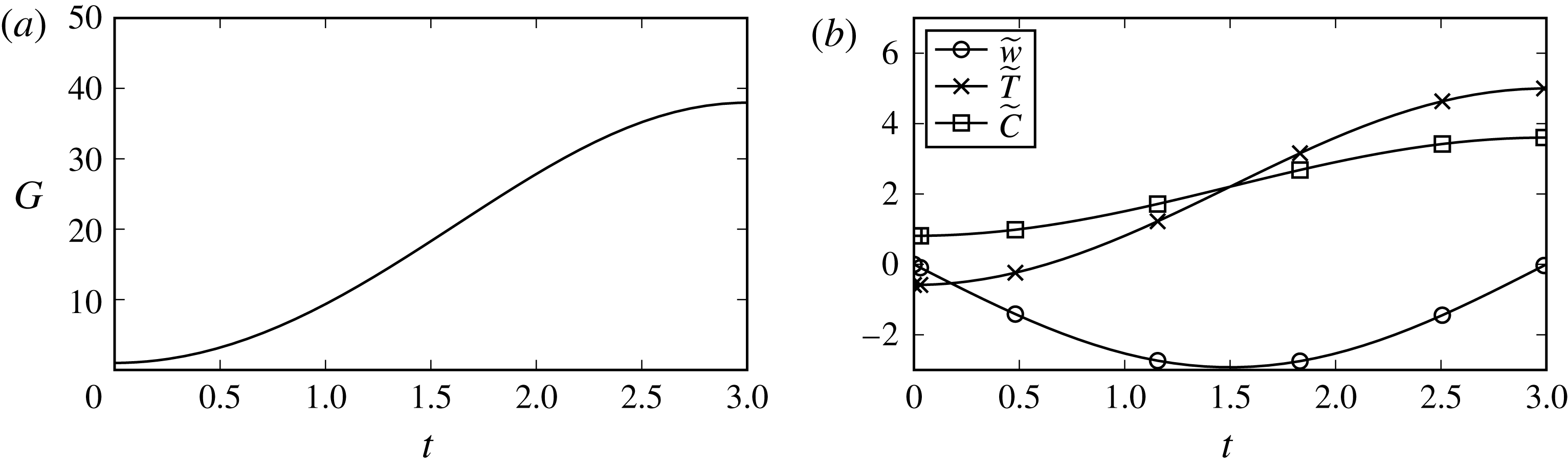
to move in the same direction until they eventually are of the same sign and sufficiently large for the transient growth to decay. A representative example is shown in figure 3, which displays the overall gain and individual solution components as functions of time for the optimal solution with
 $t_{\text{end}}=3$
and the same parameters as in figure 2. At first,
 $\widetilde{T}$
and
 $\widetilde{C}$
have opposite signs, which causes
 $\widetilde{w}$
to become negative. This negative
 $\widetilde{w}$
causes both
 $\widetilde{T}$
and
 $\widetilde{C}$
to increase. Since
 $R_{\unicode[STIX]{x1D70C}}>1$
,
 $\widetilde{w}$
affects
 $\widetilde{T}$
more strongly than
 $\widetilde{C}$
. When
 $\widetilde{T}$
and
 $\widetilde{C}$
cross,
 $\widetilde{w}$
stops growing and begins to decay. The overall gain continues to increase until the point where
 $\widetilde{w}=0$
, at which point
 $\widetilde{T}$
and
 $\widetilde{C}$
would begin to decrease.
The optimally growing solution for
 $t_{\text{end}}=3$
with
 $Pr=7$
,
 $\unicode[STIX]{x1D70F}=100$
,
 $R_{\unicode[STIX]{x1D70C}}=2$
,
 $V_{p}=0$
and
 $S=0$
. (a) The gain
 $G$
, and (b) the solution components. Here the solution is real.

This transient growth mechanism relies on the existence of density gradients, and it occurs whether or not shear is present. This is in contrast to the Orr mechanism (Lindzen Reference Lindzen1988), which requires shear and does not depend on density gradients. The Orr mechanism is related to the tilting of the plane perturbation vorticity wave by the background shear. If this wave is initially tilted against the shear, its vorticity contours are relatively close together. As
 $m$
decreases with time due to the shear and the perturbation wave tilts into an upright position, the vorticity contours separate. Since the strength of the perturbation vorticity wave is conserved during this tilting process, the kinetic energy of the associated perturbation velocity field increases. As the background shear tilts the wave past the upright position, the perturbation vorticity contours come closer together again, and the associated kinetic energy decreases. The maximum gain due to this inviscid Orr mechanism can be found by considering the relationship between vorticity and vertical velocity, which can be derived from the definition of vorticity and continuity
 $$\begin{eqnarray}\displaystyle {\displaystyle \frac{\unicode[STIX]{x2202}\unicode[STIX]{x1D714}}{\unicode[STIX]{x2202}x}}=\unicode[STIX]{x1D6FB}^{2}w. & & \displaystyle\end{eqnarray}$$
By substituting the time dependent plane wave (2.29) into this equation, we obtain
 $$\begin{eqnarray}\displaystyle & \displaystyle \widetilde{w}=-{\displaystyle \frac{\text{i}k}{k^{2}+(m_{0}-Skt)^{2}}}\widetilde{\unicode[STIX]{x1D714}}. & \displaystyle\end{eqnarray}$$
The maximum
 $\widetilde{w}$
will occur when
 $t=m_{0}/(Sk)$
, i.e. when
 $m=0$
and the wave is vertical. The associated maximum gain is
 $$\begin{eqnarray}\displaystyle & \displaystyle G_{w}={\displaystyle \frac{|\widetilde{w}|^{2}|_{t=t_{\text{end}}}}{|\widetilde{w}|^{2}|_{t=0}}}={\displaystyle \frac{(k^{2}+m_{0}^{2})^{2}}{k^{4}}}, & \displaystyle\end{eqnarray}$$
where
 $G_{w}$
differs from
 $G$
in (3.1) in that
 $G_{w}$
only contains
 $\widetilde{w}$
and not
 $\widetilde{T}$
and
 $\widetilde{C}$
, and the second equality reflects the fact that the vorticity of a fluid element is conserved over time. If
 $m_{0}\neq 0$
, this means that the inviscid Orr mechanism would result in infinite gain as the optimizer chooses smaller and smaller
 $k$
, which is the same limit that drives the transient growth mechanism described earlier. At this point one may wonder why the gain does not become infinite for cases with shear as
 $k\rightarrow 0$
. To answer this question, we need to consider the time it takes for shear to tilt the wave into the upright position
 $$\begin{eqnarray}\displaystyle & \displaystyle t={\displaystyle \frac{m_{0}}{Sk}}, & \displaystyle\end{eqnarray}$$
which is the time it takes for the vertical wavenumber
 $m$
to decrease from
 $m_{0}$
initially to 0. For any given finite value of
 $m_{0}$
, we can make
 $k$
small enough to make the gain as large as we like. However, as
 $k\rightarrow 0$
, the time until the infinite gain is realized becomes infinite. At this point, it becomes helpful to include the effects of viscosity. Since viscous forces would have an infinite amount of time to dampen the Orr mechanism, it is not immediately obvious whether infinite gain can be achieved in the presence of viscosity. We begin by considering the ODE for
 $\widetilde{w}$
in an unstratified two-dimensional case with viscosity
 $$\begin{eqnarray}\displaystyle & \displaystyle {\displaystyle \frac{\text{d}\widetilde{w}}{\text{d}t}}=\left(-Pr(k^{2}+(m_{0}-Skt)^{2})+{\displaystyle \frac{2Sk(m_{0}-Skt)}{k^{2}+(m_{0}-Skt)^{2}}}\right)\widetilde{w}. & \displaystyle\end{eqnarray}$$
This ODE can be obtained from (2.37) by neglecting
 $\widetilde{T}$
and
 $\widetilde{C}$
. The analytical solution is
 $$\begin{eqnarray}\displaystyle & \displaystyle \widetilde{w}(t)=\widetilde{w}(0)\exp \left[-\int _{0}^{t}Pr(k^{2}+(m_{0}-Skt^{\prime })^{2})\,\text{d}t^{\prime }\right]\exp \left[\int _{0}^{t}{\displaystyle \frac{2Sk(m_{0}-Skt^{\prime })}{k^{2}+(m_{0}-Skt^{\prime })^{2}}}\,\text{d}t^{\prime }\right]. & \displaystyle \nonumber\\ \displaystyle & & \displaystyle\end{eqnarray}$$
We know from our analysis of the inviscid problem that the maximum value of the second exponential is
 $(k^{2}+m_{0}^{2})/k^{2}$
and occurs when
 $t=m_{0}/(Sk)$
. This value is the square root of the maximum gain from (4.4). We can evaluate the first integral, which expresses the influence of viscosity, at
 $t=m_{0}/(Sk)$
to complete the expression
 $$\begin{eqnarray}\displaystyle & \displaystyle {\displaystyle \frac{\widetilde{w}\left({\displaystyle \frac{m_{0}}{Sk}}\right)}{\widetilde{w}(0)}}=\exp \left[-{\displaystyle \frac{(3k^{2}m_{0}+m_{0}^{3})Pr}{3Sk}}\right]{\displaystyle \frac{k^{2}+m_{0}^{2}}{k^{2}}}. & \displaystyle\end{eqnarray}$$
This expression for the growth of the viscous Orr mechanism was also derived by Craik & Criminale (Reference Craik and Criminale1986). If we take the limit of (4.8) as
 $k\rightarrow 0$
with
 $m_{0}>0$
, we see that the gain will become zero because the exponential decay dominates. However, if we choose a relation between
 $k$
and
 $m_{0}$
of the form
 $$\begin{eqnarray}\displaystyle k=Cm_{0}^{n} & & \displaystyle\end{eqnarray}$$
where
 $C$
and
 $n$
are constants, and substitute that into (4.8), we obtain
 $$\begin{eqnarray}\displaystyle & \displaystyle \frac{\widetilde{w}\left({\displaystyle \frac{m_{0}}{Sk}}\right)}{\widetilde{w}(0)}=\exp \left[-{\displaystyle \frac{(3C^{2}m_{0}^{2n-2}+1)Pr}{3SCm_{0}^{n-3}}}\right]{\displaystyle \frac{C^{2}m_{0}^{2n-2}+1}{C^{2}m_{0}^{2n-2}}}. & \displaystyle\end{eqnarray}$$
The rightmost fraction in this equation shows us that if we wish to obtain infinite gain as
 $m_{0}\rightarrow 0$
, we need to choose
 $n>1$
, but this would mean that infinite time would be required to realize that infinite gain, seen in (4.5). Alternatively, we can choose
 $n=1$
and have an arbitrarily large gain as
 $C\rightarrow 0$
. However, equation (4.5) shows that after choosing
 $n=1$
and substituting
 $k=Cm_{0}$
, infinite time is required to produce the infinite gain as
 $C\rightarrow 0$
. Either way, as long as
 $n<3$
, the exponential term will approach one as
 $m_{0}\rightarrow 0$
. Consequently, viscosity will not prevent the Orr mechanism from producing infinite gain, but infinite time will also be required to produce the infinite gain.
We can use (4.4), (4.5) and (4.9) to construct a function that gives the maximum gain from the inviscid Orr mechanism as a function of
 $t_{\text{end}}$
. Substituting (4.9) in (4.5) gives
 $C=1/(St_{\text{end}}m_{0}^{n-1})$
. This is the
 $C$
-value that corresponds to the wave with
 $k$
and
 $m_{0}$
that the Orr mechanism can tilt into a fully upright position by time
 $t_{\text{end}}$
. Setting
 $k=Cm_{0}^{n}$
and
 $C=1/(St_{\text{end}}m_{0}^{n-1})$
in (4.4) gives
 $$\begin{eqnarray}\displaystyle G_{w}=(1+S^{2}{t_{\text{end}}}^{2})^{2}. & & \displaystyle\end{eqnarray}$$
In this paper, we study the effects of shear by setting
 $S=0.1$
. This means that the Orr mechanism will require a long time to produce large gain as
 $k\rightarrow 0$
and
 $m_{0}\rightarrow 0$
, even in the absence of viscosity. For the times that we considered, the growth of the settling or fingering instability was always larger than the growth of the Orr mechanism as
 $k\rightarrow 0$
and
 $m_{0}\rightarrow 0$
. We note that this does not imply that the Orr mechanism is generally irrelevant, as there are cases when it can enhance the gain caused by the instability. In order to clarify this issue, the relative importance of the instability growth and the Orr mechanism will be discussed and compared in the following §§ 4.2.2 and 4.3.3.
4.2 Effect of shear on the fingering instability
To study the gain of the fingering instability with and without shear, we analyse the case of
 $Pr=7$
,
 $\unicode[STIX]{x1D70F}=100$
,
 $R_{\unicode[STIX]{x1D70C}}=2$
and
 $V_{p}=0$
, for
 $S=0$
and
 $0.1$
, respectively. Figure 2 shows the optimal gain
 $G$
as a function of time
 $t_{\text{end}}$
, along with the
 $k$
- and
 $m_{0}$
-values that produce this gain. Without shear, the optimally growing mode has
 $m=m_{0}=0$
and produces roughly exponential growth beyond the transient phase. The growth rate and most amplified
 $k$
-value from linear stability theory (Alsinan et al.
Reference Alsinan, Meiburg and Garaud2017), also shown in figure 2, agree closely with the gain obtained from the present analysis. Since the mode with
 $m=0$
has no dependence on
 $z$
, it is commonly referred to as the ‘elevator mode’. With shear, the gain is smaller and
 $m_{0}>0$
. Larger times
 $t_{\text{end}}$
result in larger initial values
 $m_{0}$
, so that the flow can spend most of the time interval over which the gain is evaluated near
 $m=0$
, where the fingering instability experiences maximum growth. Having
 $m_{0}>0$
also allows for the Orr mechanism to provide some additional growth. Since for
 $l=0$
the shear reduces the gain of modes with
 $k>0$
, the discussion at the beginning of § 3 suggests that for the fingering case with shear optimal growth will occur for
 $k=0$
and
 $l>0$
, which corresponds to a salt sheet. This is consistent with previous work on the interaction of the fingering instability with shear (Linden Reference Linden1974; Smyth & Kimura Reference Smyth and Kimura2007, Reference Smyth and Kimura2011; Radko et al.
Reference Radko, Ball, Colosi and Flanagan2015).
4.2.1 Influence of
 $\unicode[STIX]{x1D70F}$
and
$R_{\unicode[STIX]{x1D70C}}$


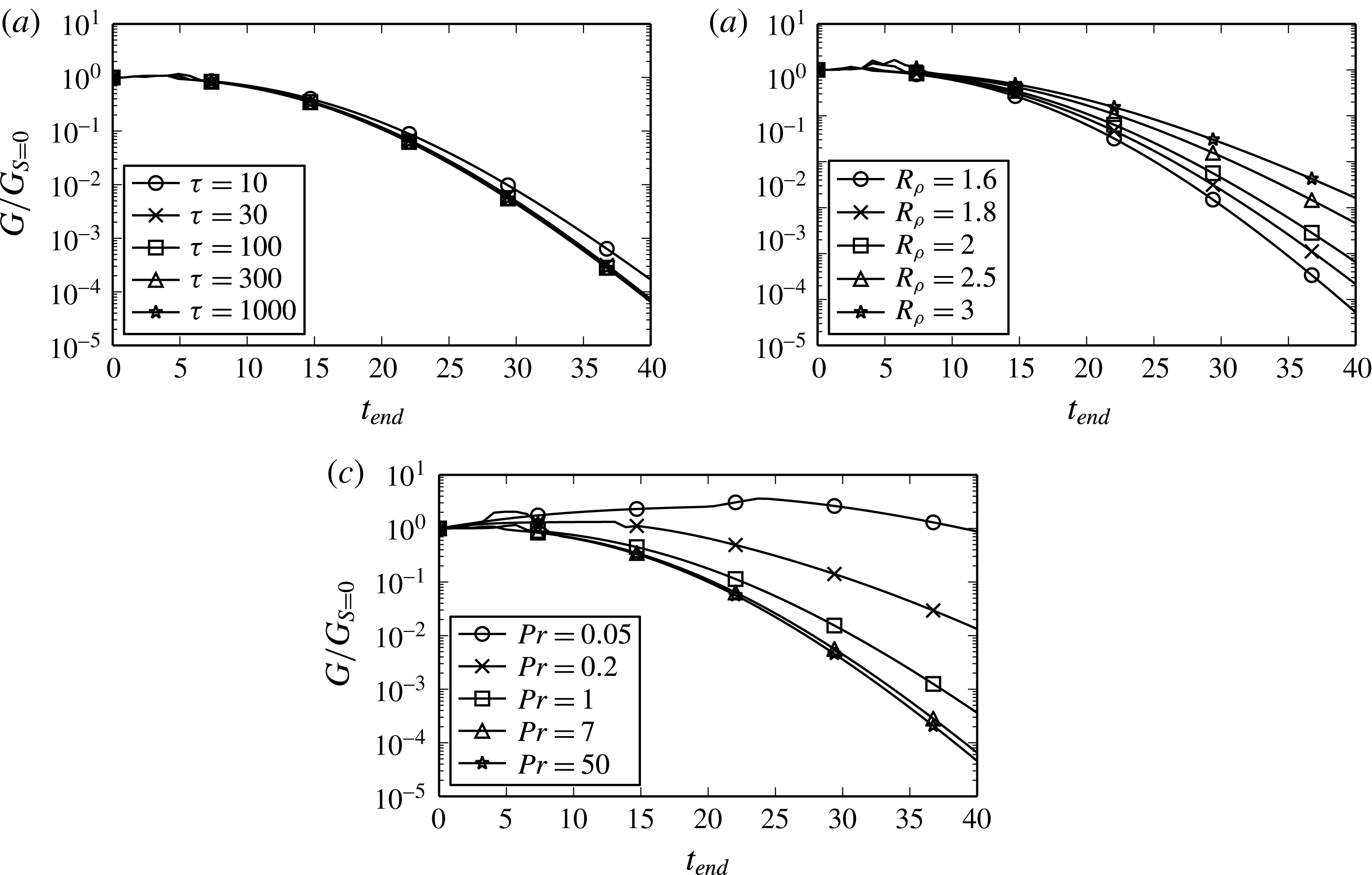
Ratio of sheared optimal gain with
 $S=0.1$
to unsheared optimal gain for the fingering instability. Unless noted otherwise in the legend, the parameter values are
 $Pr=7$
,
 $\unicode[STIX]{x1D70F}=100$
,
 $R_{\unicode[STIX]{x1D70C}}=2$
and
 $V_{p}=0$
.

To determine how the damping effect of shear on the fingering instability depends on
 $\unicode[STIX]{x1D70F}$
and
 $R_{\unicode[STIX]{x1D70C}}$
, we calculate the optimal growth for the base case parameters and varying
 $\unicode[STIX]{x1D70F}$
- and
 $R_{\unicode[STIX]{x1D70C}}$
-values, for both
 $S=0$
and 0.1. Figures 4(a) and (b) show the ratio of the sheared to the unsheared gain as a function of
 $t_{\text{end}}$
for different
 $\unicode[STIX]{x1D70F}$
- and
 $R_{\unicode[STIX]{x1D70C}}$
-values. Increasing
 $\unicode[STIX]{x1D70F}$
from 10 to 1000 slightly increases the damping influence of shear. Similarly, lower values of
 $R_{\unicode[STIX]{x1D70C}}$
are affected somewhat more strongly by shear than higher values. Since lower
 $\unicode[STIX]{x1D70F}$
and higher
 $R_{\unicode[STIX]{x1D70C}}$
correspond to weaker unsheared fingering, we can summarize these trends by stating that weaker fingering generally is affected less by the presence of shear.
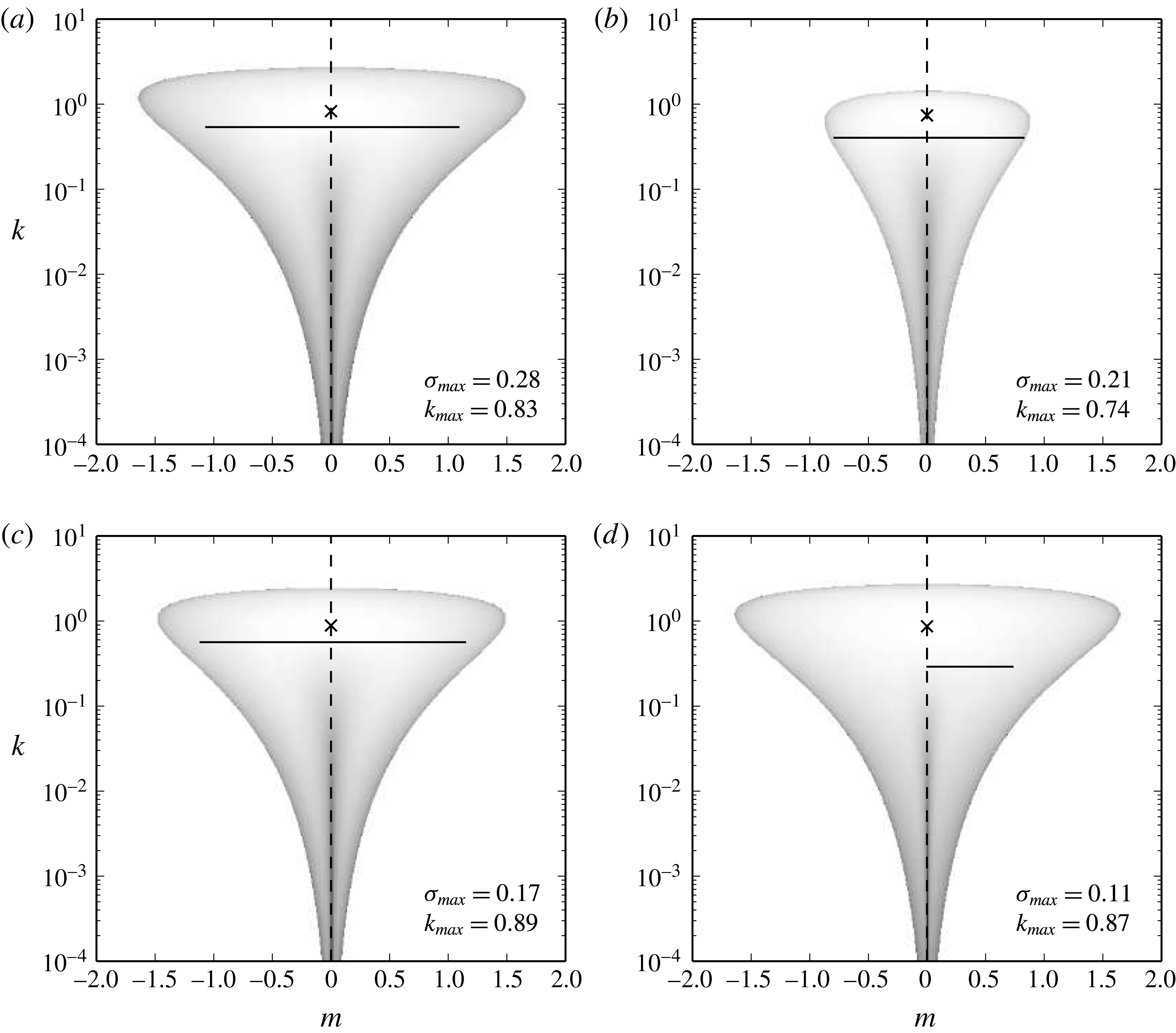
The unsheared case
 $S=0$
: linear stability analysis growth rate versus horizontal wavenumber
 $k$
and vertical wavenumber
 $m$
for the parameter combinations: (a) base case of
 $Pr=7$
,
 $\unicode[STIX]{x1D70F}=100$
,
 $R_{\unicode[STIX]{x1D70C}}=2$
and
 $V_{p}=0$
, (b) decreased
 $\unicode[STIX]{x1D70F}=10$
, (c) increased
 $R_{\unicode[STIX]{x1D70C}}=3$
and (d) decreased
 $Pr=0.05$
. The shading is logarithmic, and the maximum growth rates are marked with an X. The horizontal black lines represent the paths of the non-modal optimal growth from
 $t=0$
to
 $t_{\text{end}}$
for
 $S=0.1$
according to
 $m=m_{0}-Skt$
. (a–c):
 $t_{\text{end}}=40$
, (d) and
 $t_{\text{end}}=25$
.

These trends can be understood on the basis of the linear stability results for the case without shear. Figure 5 shows these linear stability results for (a) the base case, (b) the base case but with
 $\unicode[STIX]{x1D70F}=10$
and (c) the base case but with
 $R_{\unicode[STIX]{x1D70C}}=3$
. Without shear, as
 $t_{\text{end}}\rightarrow \infty$
the optimal growth will approach the fastest growing linearly unstable mode, as seen in figure 2. When shear is added, the vertical wavenumber
 $m$
becomes a function of
 $t$
, with
 $m(t)=m_{0}-Skt$
. For a given time horizon
 $t_{\text{end}}$
, the values that
 $m$
takes between
 $t=0$
and
 $t=t_{\text{end}}$
, starting from the optimal
 $m_{0}$
, are drawn in figure 5. Knowing this trajectory of
 $m$
in time, one can attempt a crude approximation of the final gain
 $G(t_{\text{end}})$
by integrating the corresponding growth rate
 $\unicode[STIX]{x1D70E}(k,m(t))$
from the unsheared calculations over
 $0\leqslant t\leqslant t_{\text{end}}$
,
 $$\begin{eqnarray}\displaystyle & \displaystyle G(t_{\text{end}})\approx \exp \left[\int _{0}^{t_{\text{end}}}2\unicode[STIX]{x1D70E}(k,m(t))\,\text{d}t\right], & \displaystyle\end{eqnarray}$$
where the factor
 $2$
is needed in order to account for the definition of
 $G$
as an energy gain (3.1). This approximation neglects some non-modal growth effects arising from changes of the spatial perturbation shape. A damping factor can then be computed as
 $$\begin{eqnarray}\displaystyle & \displaystyle D(t_{\text{end}})={\displaystyle \frac{G(t_{\text{end}})_{S=0.1}}{G(t_{\text{end}})_{S=0}}}=\exp \left[2\left(\int _{0}^{t_{\text{end}}}\unicode[STIX]{x1D70E}(t)-\unicode[STIX]{x1D70E}_{max}\,\text{d}t\right)\right], & \displaystyle\end{eqnarray}$$
where
 $\unicode[STIX]{x1D70E}_{max}$
is the maximum growth rate from the linear stability analysis and which serves as an approximation of the unsheared instability growth. Equation (4.13) approximates the damping influence of shear based only on knowledge of the variation
 $m(t)$
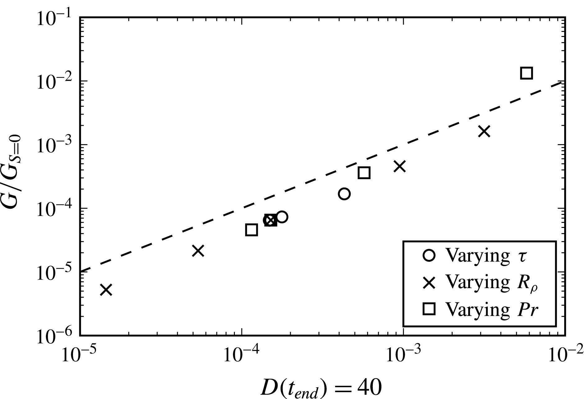
and of unsheared linear stability results. Figure 6 compares this approximate damping factor with the actual ratio
 $G(t_{\text{end}})_{S=0.1}/G(t_{\text{end}})_{S=0}$
for several variations of the baseline parameter configuration. Equation (4.13) reproduces the correct trend for the strength of the damping, which suggests that the trends of figure 4(a,b) are due to the fact that those parameter combinations for which
 $\unicode[STIX]{x1D70E}$
depends more weakly on
 $(k,m)$
are damped less by shear.
The effects of transient growth may still play a role in the imperfect agreement of figure 6, but they do not dominate the overall trends as
 $\unicode[STIX]{x1D70F}$
and
 $R_{\unicode[STIX]{x1D70C}}$
are varied. In the presence of shear, transient growth affects the solution at all times since the local eigenmodes constantly change as a result of the time dependence of
 $m(t)$
. In addition, the Orr mechanism provides a boost of
 $\widetilde{w}$
as
 $m$
crosses zero, and subsequently causes extra damping of
 $\widetilde{w}$
as
 $m$
moves away from zero.
Actual damping
 $G(S)/G_{S=0}$
for
 $S=0.1$
as a function of predicted damping (4.13) from assuming locally exponential growth as
 $m(t)=m_{0}-Skt$
changes over time. The correct trend is recovered for all parameter combinations, although the predictions are a factor of 2–3 too small. Values of
 $\unicode[STIX]{x1D70F}$
are 10, 30, 100, 300 and 1000. Values of
 $R_{\unicode[STIX]{x1D70C}}$
are 1.6, 1.8, 2, 2.5 and 3. Values of
 $Pr$
are 0.2, 1, 7 and 50.

According to (4.13), smaller values of
 $\unicode[STIX]{x1D70E}-\unicode[STIX]{x1D70E}_{max}$
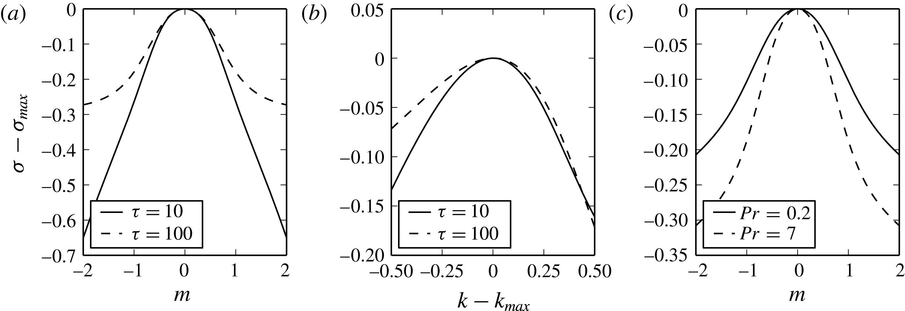
reduce the damping effect of shear. Figures 7(a) and 7(b) show the dependence of
 $\unicode[STIX]{x1D70E}-\unicode[STIX]{x1D70E}_{max}$
on
 $k$
(for
 $m=0$
) and on
 $m$
(for
 $k=k_{max}$
). Here
 $k_{max}$
is the
 $k$
-value for which
 $\unicode[STIX]{x1D70E}_{max}$
occurs. Even though figure 4(a) indicates that
 $\unicode[STIX]{x1D70F}=10$
is damped less than
 $\unicode[STIX]{x1D70F}=1000$
,
 $\unicode[STIX]{x1D70E}$
is reduced more for
 $\unicode[STIX]{x1D70F}=10$
along both of the paths shown in figures 7(a) and 7(b). This apparent contradiction is resolved by the fact that for
 $\unicode[STIX]{x1D70F}=10$
the optimized growth path proceeds along a reduced value
 $k<k_{max}$
, as seen in figure 5(b). Although
 $\unicode[STIX]{x1D70E}$
is reduced less for
 $\unicode[STIX]{x1D70F}=10$
along this path with
 $k<k_{max}$
, this would not be hypothesized from figure 7(b). The fact that
 $\unicode[STIX]{x1D70E}$
is reduced more for
 $\unicode[STIX]{x1D70F}=10$
along
 $m=0$
as
 $k$
is reduced makes it difficult to produce a physical explanation why
 $\unicode[STIX]{x1D70E}$
is reduced less along the optimal path for
 $\unicode[STIX]{x1D70F}=10$
.
In summary, while the linear stability results clearly indicate that parameter combinations giving rise to more vigorous fingering are damped more strongly by shear, the physical reasons for this stronger damping are not entirely clear.
(a)
 $\unicode[STIX]{x1D70E}-\unicode[STIX]{x1D70E}_{max}$
as a function of
 $m$
for
 $k=k_{max}$
, where
 $\unicode[STIX]{x1D70E}_{max}$
is the maximum growth rate and
 $k_{max}$
is the value of
 $k$
where
 $\unicode[STIX]{x1D70E}_{max}$
occurs. (b)
 $\unicode[STIX]{x1D70E}-\unicode[STIX]{x1D70E}_{max}$
as a function of
 $k$
with
 $m=0$
. (c)
 $\unicode[STIX]{x1D70E}-\unicode[STIX]{x1D70E}_{max}$
as a function of
 $m$
with
 $k=k_{max}$
for two values of
 $Pr$
. In (a) and (b),
 $\unicode[STIX]{x1D70E}$
is more sensitive to
 $k$
and
 $m$
when
 $\unicode[STIX]{x1D70F}=10$
compared to
 $\unicode[STIX]{x1D70F}=1000$
. Other parameters are
 $Pr=7$
,
 $R_{\unicode[STIX]{x1D70C}}=2$
and
 $V_{p}=0$
. In (c),
 $\unicode[STIX]{x1D70E}$
is more sensitive to
 $m$
when
 $Pr=7$
. The other parameters are
 $\unicode[STIX]{x1D70F}=100$
,
 $R_{\unicode[STIX]{x1D70C}}=2$
and
 $V_{p}=0$
.

4.2.2 Influence of
$Pr$

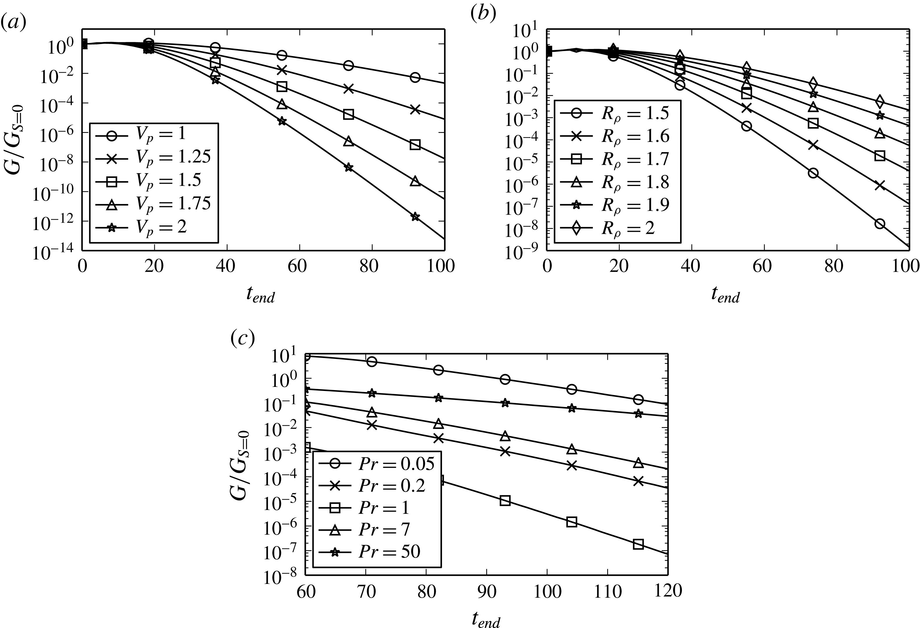
Figure 4(c) shows that shear has less of a damping effect on flows with smaller
 $Pr$
-values, and even produces additional transient growth when
 $Pr=0.05$
. As indicated by figure 6, the general trend can once again be explained in terms of linear stability analysis growth rates, with the exception of
 $Pr=0.05$
. Figure 7(c) shows that
 $\unicode[STIX]{x1D70E}$
is more sensitive to
 $m$
for high than for low
 $Pr$
, which is consistent with the fact that high
 $Pr$
flows get damped more. This allows us to formulate a physical argument for why there is less damping by shear when
 $Pr$
is small.
We recall that the fingering instability is both driven and damped by diffusion, in the following sense. Deviations from the base state in both
 $T$
and
 $C$
contribute to vorticity generation. Since
 $T$
is stably stratified, the
 $T$
-related vorticity is stabilizing. Correspondingly, since
 $C$
is unstably stratified, the
 $C$
-related vorticity has a destabilizing influence. As the relative importance of diffusion grows with increasing
 $k$
or
 $m$
, the larger diffusivity of
 $T$
causes the
 $T$
-vorticity to be damped more than the
 $C$
-vorticity, resulting in a net increase in destabilizing vorticity. In addition, as
 $k$
is increased independently of
 $m$
, the
 $(1,2)$
and
 $(1,3)$
terms in (2.37) show that vertical velocity generation grows proportionally to
 $k^{2}/(k^{2}+m^{2})$
. This effect is influential since the interaction of the vertical velocity with the background
 $T$
- and
 $C$
-gradients drives the instability.
When
 $Pr$
is reduced, vertical velocity generation and diffusion are both reduced. As the top row coefficients in (2.37) show, this results in smaller overall vertical velocity growth on the left hand side. To compensate, it becomes relatively more advantageous to increase the double-diffusive effect by increasing
 $|m|$
. Increasing
 $|m|$
accomplishes three things. Firstly, it increases the importance of diffusion, which decreases the growth rate. Secondly, because of increased diffusion, there is also a stronger double-diffusive effect, which enhances the growth rate. Thirdly, it decreases the vertical velocity production terms
 $(1,2)$
and
 $(1,3)$
in (2.37), which decreases the growth rate. The overall effect of increasing
 $|m|$
is to decrease the growth rate. When
 $Pr$
is small, increasing
 $|m|$
decreases the vertical velocity generation terms less relative to the changes in the other terms in (2.37), reducing the influence of one of the reasons why increasing
 $|m|$
lowers the growth rate. The fact that the overall growth rate is less sensitive to
 $m$
when
 $Pr$
is small causes shear to affect the solution growth less when
 $Pr$
is small.
For
 $Pr=0.05$
the sheared case grows more strongly than the unsheared one, as a result of the Orr mechanism. The solid black line in figure 5(d) indicates that for
 $Pr=0.05$
and
 $t_{\text{end}}=25$
we have
 $m(t_{\text{end}})=0$
. This means that the Orr mechanism growth is at its strongest for
 $t=t_{\text{end}}$
when
 $Pr=0.05$
. The Orr mechanism can play a more prominent role in determining the optimal growth when
 $Pr$
is low because this implies low viscosity. The reduced damping effect of viscosity on the Orr mechanism is reflected by the exponential term in (4.8). Equation (4.8) can also provide an estimate of the maximum gain from the Orr mechanism alone. Towards this end, if we assume that
 $\widetilde{T}$
and
 $\widetilde{C}$
are constant in time, the maximum gain from the Orr mechanism would be about one third the result of (4.8) squared. For the present case with
 $Pr=0.05$
and
 $t_{\text{end}}=25$
, this evaluates to about 9, which is consistent with the results in figure 5(d). For
 $Pr=0.2$
, the estimate is reduced to about 1.25, meaning that the Orr mechanism would provide much less of a boost. For
 $Pr\geqslant 0.2$
, optimal growth is achieved by having
 $m(t)$
spend roughly equal amounts of time on either side of zero, as seen in figure 5. Since this path for
 $m(t)$
is twice as long, larger
 $k$
can be accommodated with
 $\text{d}m/\text{d}t=-Sk$
. Because these larger
 $k$
-values produce stronger growth, their overall growth is higher without relying on the Orr mechanism.
4.3 Effect of shear on the settling instability
Optimized gain
 $G$
and corresponding
 $k$
and
 $m_{0}$
as a function of time interval
 $[0,t_{\text{end}}]$
for the settling instability. The other parameters are
 $Pr=7$
,
 $\unicode[STIX]{x1D70F}=1$
,
 $R_{\unicode[STIX]{x1D70C}}=2$
and
 $V_{p}=1$
. The dotted lines indicate linear stability results for maximum growth rate and corresponding
 $(k,m)$
, in the absence of shear.

In order to investigate the effect of shear on the settling-driven instability (Alsinan et al.
Reference Alsinan, Meiburg and Garaud2017), we set
 $\unicode[STIX]{x1D70F}=1$
to eliminate any double-diffusive effects. For the case of
 $Pr=7$
,
 $R_{\unicode[STIX]{x1D70C}}=2$
and
 $V_{p}=1$
, figure 8 shows that shear dampens the settling-driven instability, just as it dampens the fingering instability. Recall that the streamwise salt sheets discussed above in the context of the double-diffusive instability were oriented vertically, since the unsheared instability favours the
 $m=0$
mode. For the settling-driven instability the situation is quite different. Since now
 $m\neq 0$
for the unsheared case, the ‘particle sheets’ will be tilted in the spanwise direction. The linear stability analysis of Alsinan et al. (Reference Alsinan, Meiburg and Garaud2017) furthermore showed that the unsheared case favours two equally unstable modes with opposite wave slopes for the settling-driven instability. DNS simulations by the same authors indicated that both of these modes are present, resulting in a criss-cross pattern of waves. Hence we predict that in a three-dimensional flow with shear acting in the
 $x,z$
-plane the initially dominant settling-driven instability mode will have the shape of this criss-cross pattern in the
 $y,z$
-plane, while being invariant in the
 $x$
-direction. This will give rise to ‘tube-like’ structures, rather than sheets. In the following sections we examine the quantitative effect of shear on various aspects of the settling-driven instability.
4.3.1 Influence of
$V_{p}$

To determine how the effect of shear depends on the settling velocity, which acts as proxy for the particle size, we calculate the maximum gain with
 $S=0$
and 0.1, and for
 $V_{p}=(1,1.25,1.5,1.75,2)$
. The ratio of the sheared to the unsheared gain displayed in figure 9 demonstrates that the effect of shear on the settling-driven instability increases with
 $V_{p}$
.
Ratio of sheared optimal gain with
 $S=0.1$
to unsheared optimal gain for the settling instability with
 $\unicode[STIX]{x1D70F}=1$
. Other parameters are (a)
 $Pr=7$
,
 $R_{\unicode[STIX]{x1D70C}}=2$
, (b)
 $Pr=7$
,
 $V_{p}=1$
, (c)
 $R_{\unicode[STIX]{x1D70C}}=2$
,
 $V_{p}=1$
.

In order to explain this trend, we first review the mechanism behind the settling-driven instability as originally discussed in Alsinan et al. (Reference Alsinan, Meiburg and Garaud2017). Again we have stabilizing
 $T$
- and destabilizing
 $C$
-vorticity. Since temperature contributes more strongly to the density, and the overall background density gradient is stable, the
 $T$
-vorticity will outweigh the
 $C$
-vorticity if the
 $T$
- and
 $C$
-perturbations have the same phase and diffuse at the same rate (
 $\unicode[STIX]{x1D70F}=1$
), so that the system will be stable. When
 $V_{p}>0$
, on the other hand, a phase shift is introduced between the
 $T$
- and
 $C$
-perturbations, so that the stabilizing
 $T$
-vorticity does not outweigh the destabilizing
 $C$
-vorticity everywhere. This provides the conditions for an instability to develop.
Based on this explanation, it would be fair to wonder why
 $V_{p}>0$
is needed for this instability to occur. In principle, a phase offset can be introduced in the initial perturbations of
 $T$
and
 $C$
, so that the
 $T$
-vorticity does not stabilize the flow everywhere even when
 $V_{p}=0$
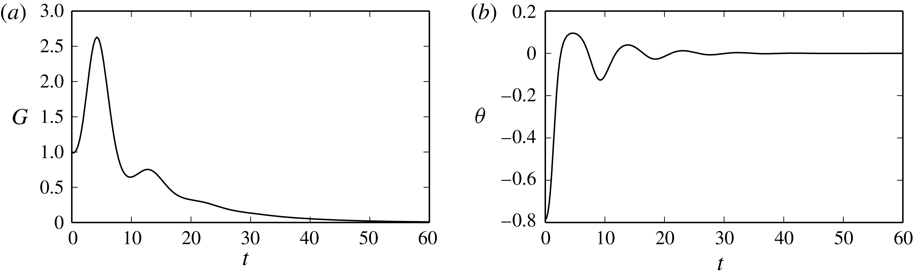
. But as we know from linear stability analysis, the resulting flow is still stable. The reason for this is that, even though an initial phase shift produces some transient growth, the resulting flow acts in such a way as to gradually reduce the phase offset between the
 $T$
- and
 $C$
-perturbations, so that these perturbations decay for long times. This is illustrated in figure 10, which shows the gain
 $G$
and phase angle
 $\unicode[STIX]{x1D703}$
between the
 $T$
- and
 $C$
-perturbations as functions of time for a case with
 $V_{p}=0$
,
 $\unicode[STIX]{x1D70F}=1$
,
 $k=0.08$
,
 $m=0.2$
and an initial phase angle of
 $\unicode[STIX]{x1D703}(0)=-\unicode[STIX]{x03C0}/4$
. The traditional linear stability analysis, such as applied by Alsinan et al. (Reference Alsinan, Meiburg and Garaud2017), captures only the long-term behaviour.
(a) Gain, as defined in (3.1), and (b) phase angle between temperature and particle perturbations as functions of time for
 $Pr=7$
,
 $\unicode[STIX]{x1D70F}=1$
,
 $R_{\unicode[STIX]{x1D70C}}=2$
,
 $V_{p}=0$
and initial
 $\unicode[STIX]{x1D703}=-\unicode[STIX]{x03C0}/4$
. There is initial, transient growth that decays as the phase angle decays without any sustained driving force to maintain it.

We can further examine the source of this phase angle decay by considering an inviscid case without diffusion of either scalar, and in the absence of settling. In this scenario, the phase angle will decay initially, overshoot zero, reach a new maximum of opposite sign, decay again and overshoot zero to return to the initial position, only to restart the oscillation. Since there is no viscosity or diffusion, this oscillation is undamped. When viscosity and diffusion are added, the oscillations become damped with a viscous decay rate of
 $-(k^{2}+m^{2})$
, according to the eigenvalues of the matrix in (2.37) with
 $S=0$
,
 $V_{p}=0$
and
 $\unicode[STIX]{x1D70F}=1$
. The two oscillatory eigenmodes with phase offset between
 $T$
and
 $C$
each decay with a rate of
 $-(1+Pr)(k^{2}+m^{2})/2$
. This demonstrates that if
 $k$
or
 $m$
are increased for the settling-driven instability, not only will viscous forces dampen the instability, but the phase offset which drives the instability will also have a stronger natural decay and therefore tend to be smaller.
The settling velocity
 $V_{p}$
thus provides the mechanism that sustains the phase shift between the
 $T$
- and
 $C$
-perturbations, against its natural reduction in the absence of settling. We can get an idea of how strong the effect of
 $V_{p}$
is by examining the rate of change of the phase angle between
 $T$
and
 $C$
when the
 $C$
wave is settling with speed
 $V_{p}$
. Assuming a plane wave of form
 $\text{e}^{\text{i}kx+\text{i}mz+\unicode[STIX]{x1D70E}t}$
, in order to obtain a vertical phase speed of
 $V_{p}$
at
 $x=\text{const}.$
We require
 $\unicode[STIX]{x1D70E}_{\text{i}}/m=V_{p}$
, where the imaginary part of
 $\unicode[STIX]{x1D70E}_{\text{i}}$
of the growth rate also represents the rate of change of the phase offset. Thus, the driving force for the phase offset is seen to be proportional to
 $V_{p}m$
.
For a given
 $V_{p}$
with
 $\unicode[STIX]{x1D70F}=1$
, the growth of the settling instability is then governed by a balance of three mechanisms: (a) the phase offset, governed by the balance of wave settling with strength
 $V_{p}m$
and phase offset decay with strength
 $(1+Pr)(k^{2}+m^{2})/2$
, (b) viscosity and diffusion, proportional to
 $k^{2}+m^{2}$
, which dampen the perturbations and (c)
 $k^{2}/(k^{2}+m^{2})$
, which affects the strength of the vertical velocity generated by the perturbations, according to (2.37). A smaller
 $k$
implies an effectively weaker influence of viscosity along with a larger phase offset, but also weaker velocity generation, and thus can result in very slow growth.
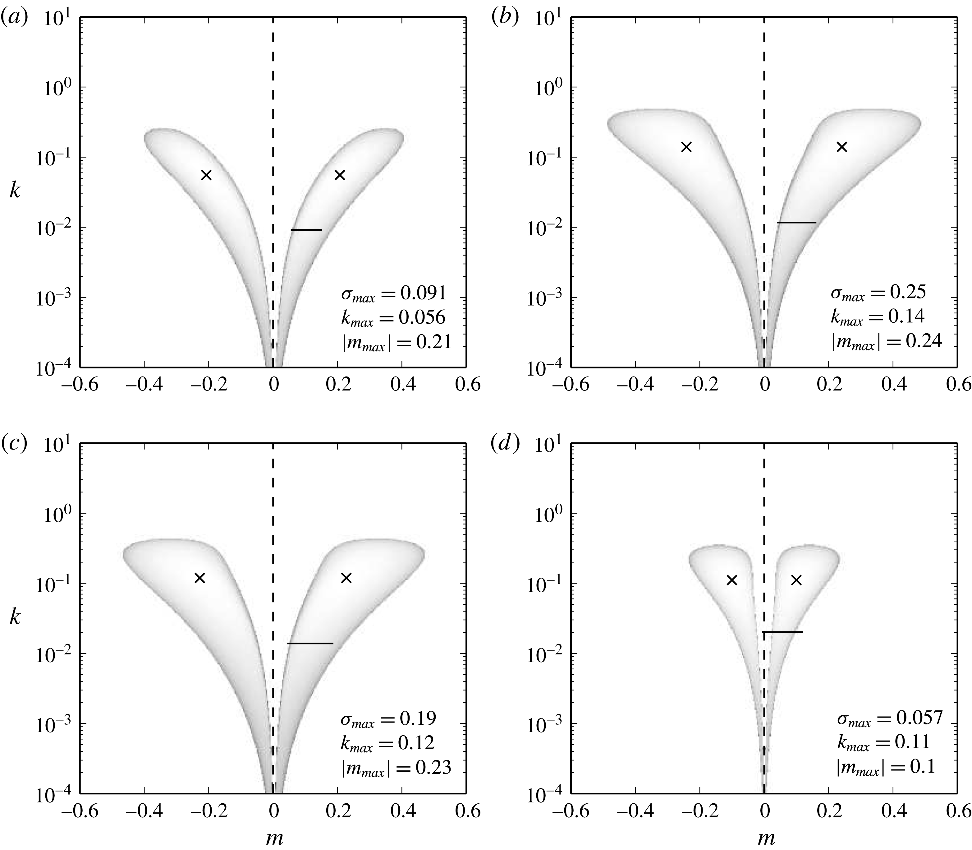
Figures 11(a) and 11(b) show the linear stability growth rates for
 $V_{p}=1$
and 2, in the absence of shear. When
 $V_{p}$
increases, for
 $m\approx \text{const.}$
we can increase
 $k$
and still have a sufficiently strong driving force
 $V_{p}m$
to maintain the phase offset, even though its natural decay increases. This larger
 $k$
increases the effect of viscosity, but also the generation of vertical velocity. This allows modes with larger
 $k$
to be unstable when
 $V_{p}$
increases, so that the instability is shifted towards larger
 $k$
, as seen in figures 11(a) and 11(b).
Linear stability growth rate versus horizontal wavenumber
 $k$
and vertical wavenumber
 $m$
in the absence of shear, for parameters (a) base case of
 $Pr=7$
,
 $\unicode[STIX]{x1D70F}=1$
,
 $R_{\unicode[STIX]{x1D70C}}=2$
and
 $V_{p}=1$
, (b) increased
 $V_{p}=2$
, (c) decreased
 $R_{\unicode[STIX]{x1D70C}}=1.5$
and (d) decreased
 $Pr=0.05$
. Shading is logarithmic. The maximum growth rates are marked with an X. The horizontal black lines represent the paths of the non-modal optimal growth when
 $S=0.1$
and
 $t_{\text{end}}=100$
(a–c), and
 $t_{\text{end}}=60$
(d), as
 $m=m_{0}-Skt$
.

We are now in a position to explain why the damping effect of shear is more pronounced for larger
 $V_{p}$
. As for the fingering instability, this can be understood in terms of the linear stability growth rates for unsheared flows. In order to produce optimal growth, the values of
 $(k,m)$
should remain inside the linearly unstable region as
 $m$
decreases with time. Figures 11(a) and 11(b) indicate that this is indeed the case for
 $V_{p}=1$
and 2. These figures also show that for larger
 $V_{p}$
the maximum growth for the unsheared flow occurs at higher
 $k$
. Recall that with shear
 $m(t)=m_{0}-Skt$
, so that
 $m$
decreases more quickly for higher
 $k$
, which means the flow spends less time in the unstable region. Consequently, the optimal growth with shear is found for
 $k$
-values somewhat below the maximum unsheared growth, for which the flow gets to spend more time in the unstable region. For
 $V_{p}=2$
and shear,
 $k$
decreases farther below the unsheared optimal
 $k$
than for
 $V_{p}=1$
, so that the growth is reduced more strongly.
4.3.2 Influence of
$R_{\unicode[STIX]{x1D70C}}$

Figure 9(b) shows that lower values of
 $R_{\unicode[STIX]{x1D70C}}$
are affected more strongly by shear than higher values. Figures 11(a) and 11(c) indicate that when
 $R_{\unicode[STIX]{x1D70C}}$
is decreased, the linear instability of the unsheared flow responds similarly to when
 $V_{p}$
is increased, and the unstable region shifts toward larger
 $k$
. To keep
 $m$
in the unstable region over time for smaller
 $R_{\unicode[STIX]{x1D70C}}$
when shear is present,
 $k$
needs to be reduced further below its unsheared maximum than for larger
 $R_{\unicode[STIX]{x1D70C}}$
, so that the growth is dampened more strongly.
The only remaining question is why for smaller
 $R_{\unicode[STIX]{x1D70C}}$
the instability shifts to larger
 $k$
. Decreasing
 $R_{\unicode[STIX]{x1D70C}}$
increases the strength of the destabilizing
 $C$
-vorticity relative to the stabilizing
 $T$
-vorticity. This means that less phase offset is required to generate an instability for smaller
 $R_{\unicode[STIX]{x1D70C}}$
. Hence the instability shifts toward larger
 $k$
-values, which generate more vorticity and faster growth, as long as
 $k$
is not so large that viscosity becomes dominant or the phase offset too small. This relationship is reflected by table 1 which shows that, compared to the base case of
 $R_{\unicode[STIX]{x1D70C}}=2$
and
 $V_{p}=1$
, reducing
 $R_{\unicode[STIX]{x1D70C}}$
to 1.5 decreases the phase offset between the temperature and particle concentration perturbations for the most unstable mode. By contrast, holding
 $R_{\unicode[STIX]{x1D70C}}=2$
constant and increasing
 $V_{p}$
to 2 drives the phase offset to larger values. This is consistent with the arguments of the previous section.
Phase angle (radians) between temperature and particle concentration waves for the most unstable mode from linear stability analysis. Other parameters are
 $Pr=7$
and
 $\unicode[STIX]{x1D70F}=1$
.

4.3.3 Influence of
$Pr$

Figure 9(c) indicates that the strength of the shear’s damping effect depends on
 $Pr$
in a non-monotonic fashion. The damping is most pronounced for
 $Pr=1$
, while it decreases for both smaller and larger
 $Pr$
-values. Consistent with our earlier observations, for
 $Pr=0.05$
shear even causes additional growth for a range of
 $t_{\text{end}}$
. We note that for some
 $Pr$
-values the settling instability grows quite slowly, so that for
 $t_{\text{end}}<60$
the initial transient growth mechanism is responsible for the maximum gain. Our interest, on the other hand, focuses on the effect of shear on the settling instability, so that we choose the range of
 $t_{\text{end}}$
in figure 9(c) as
 $[60,120]$
instead of
 $[0,100]$
.
The reduced damping when
 $Pr$
is increased from 1 can be explained on the basis of arguments from the earlier sections. Recall that the strength of the natural phase offset decay is
 $(1+Pr)(k^{2}+m^{2})/2$
. This means that increasing
 $Pr$
-values will result in smaller phase offsets and maximum growth rates for lower
 $k$
-values. Although this is not shown in figure 11, we confirmed that as
 $Pr$
increases from 1 to 7 to 50, the
 $k$
-value of the fastest growing mode in the linear stability analysis decreases from 0.140 to 0.0557 to 0.0279. As before, a lower
 $k$
for the unsheared instability leads to less damping in the presence of shear, as
 $m=m_{0}-Skt$
is able to remain inside the linearly unstable region for longer times.
When
 $Pr$
is decreased from 1, the reduced damping results from a combination of effects. Firstly, the
 $k$
-value of the fastest growing linearly unstable mode decreases from
 $0.140$
for
 $Pr=1$
, to
 $0.111$
for
 $Pr=0.05$
. Velocity generation increases with
 $k$
, but this effect is multiplied by
 $Pr$
. When
 $Pr$
becomes very low, increasing
 $k$
no longer results in as large of an increase in velocity generation relative to the other terms in (2.37). While velocity diffusion also decreases with decreasing
 $Pr$
, equation (2.37) shows that the overall growth of the velocity wave in the time derivative scales with
 $Pr$
. It is important to keep in mind that while velocity diffusion decreases, scalar diffusion does not decrease. If this seems surprising, it is because of the way we have scaled the problem. The length scale is a diffusive scale based on the temperature diffusivity. Hence for a constant problem size, varying
 $Pr$
means changing the viscosity of the fluid, not the diffusivity of the scalars. Since scalar diffusion is constant as
 $Pr$
is decreased and velocity generation is less effective at large
 $k$
for low
 $Pr$
, it becomes relatively more costly for the instability to have a higher
 $k$
. As
 $k$
becomes smaller, the phase offset decay decreases. Consequently, the effect of diffusion can be further reduced by making
 $m$
smaller as well, since less driving from the settling is needed to maintain the phase offset. In turn, smaller
 $m$
results in stronger velocity production, which scales with
 $k^{2}/(k^{2}+m^{2})$
, as mentioned earlier. The overall effect of making
 $Pr$
very small is to shift the unsheared instability toward slightly smaller
 $k$
and significantly smaller
 $m$
, as seen in figure 11(d).
This leads to the second reason why damping is decreased for smaller
 $Pr$
-values. Recall that the Orr mechanism produces maximum gain for
 $m=0$
at
 $t=t_{\text{end}}$
. Because for
 $Pr=0.05$
the instability is located closer to
 $m=0$
than for
 $Pr=1$
, as seen in figure 11(d), it becomes easier for the Orr mechanism to have an impact, as
 $m$
does not have to spend much time outside of the region of instability in order to reach zero. This is also illustrated in figure 11(d), which shows the range of
 $m$
-values over time for the optimally growing solution with
 $t_{\text{end}}=60$
and
 $Pr=0.05$
. For the fingering instability the unstable region extends all the way to
 $m=0$
, as seen in figure 5. Nevertheless, the Orr mechanism is weaker for the fingering instability than for the settling-driven instability, since
 $k$
is much larger for the fingering case. Equation (4.4) indicates that this limits the growth due to the Orr mechanism. Equation (4.8) furthermore shows that the viscous decay of the Orr mechanism is reduced for smaller
 $Pr$
, which further enhances its importance. For
 $Pr=0.05$
and
 $t_{\text{end}}=60$
, the estimate from § 4.2.2 of the maximum gain due to the Orr mechanism yields about 400. This suggests that, even though shear may dampen the settling-driven instability, the Orr mechanism may still result in enhanced overall growth for small
 $Pr$
-values, consistent with figure 9(c). For
 $Pr=0.2$
, the estimate yields a gain from the Orr mechanism alone of about 90. In summary, for
 $Pr<1$
a further decrease of
 $Pr$
will result in less damping, because the instability is located at lower
 $k$
and the Orr mechanism will contribute more to its growth, thereby leading to the larger gains seen in figure 9(c).
5 Discussion and conclusions
The present investigation assesses the effects of shear on double-diffusive fingering and on the recently identified settling-driven instability by means of a transient growth analysis. Towards this end, it employs Kelvin waves within a linearized framework, so that the evolution of time-dependent waveforms in uniform shear can be considered. This approach allows us to eliminate the effects of boundaries and of shear-driven instability modes, so that the influence of shear on the above-mentioned instabilities can be analysed in isolation.
Our analysis uses transient Kelvin waves to shed new light on the interaction of shear with the double-diffusive fingering instability. Consistent with previous analyses by other authors, we find that shear dampens the fingering instability. Our analysis is also extended to the settling-driven instability, where it shows that shear again has a dampening effect. For both of these, the shear damping is stronger for parameter combinations that produce larger unsheared growth. These trends can largely be explained in terms of instantaneous linear stability results for the unsheared case. As the vertical wavenumber
 $m(t)$
changes with time, the path of
 $(k,m(t))$
taken by the tilting Kelvin wave results in lower average growth as compared to the maximum growth rate of the unsheared case. For both instabilities, low
 $Pr$
-values result in less damping and an increased importance of the Orr mechanism. This stronger influence of the Orr mechanism can be traced to the smaller viscosity at lower
 $Pr$
. For the settling-driven instability, lower
 $Pr$
-values furthermore move the region of linear instability closer to
 $m=0$
, which strengthens the ability of the Orr mechanism to reinforce the instability.
We emphasize that the present study is limited to the linear regime, and that nonlinearities are expected to introduce new coupling mechanisms which cannot be accounted for by a linearized investigation. In particular, if the imposed shear velocity profile itself is unstable with regard to Kelvin–Helmholtz instabilities, these instabilities will likely trigger novel effects that are not captured here. The present linear analysis provides insight into the mechanisms governing the previously known damping effect of imposed shear on double-diffusive fingering, and it demonstrates that shear also stabilizes the recently identified settling-driven instability.
Although shear dampens the growth of both the double-diffusive and the settling-driven instabilities, substantial growth may still occur during the linearized phase, as seen in figures 2 and 8, so that initially small perturbations can become sufficiently large for nonlinear effects to take over. This is consistent with the findings of Smyth & Kimura (Reference Smyth and Kimura2011) and Radko et al. (Reference Radko, Ball, Colosi and Flanagan2015). We expect a similar situation for the settling-driven instability, for which the shear dampening effect is of the same order, as seen in figures 4 and 9. However, this scenario will have to be analysed in more depth by means of nonlinear simulations.
Acknowledgements
The authors thank Dr T. Koellner for helpful discussions on adjoint-based optimization. Financial support was received through NSF grant CBET-1438052, as well as grant DN NSWC N00174-16-C-0013.