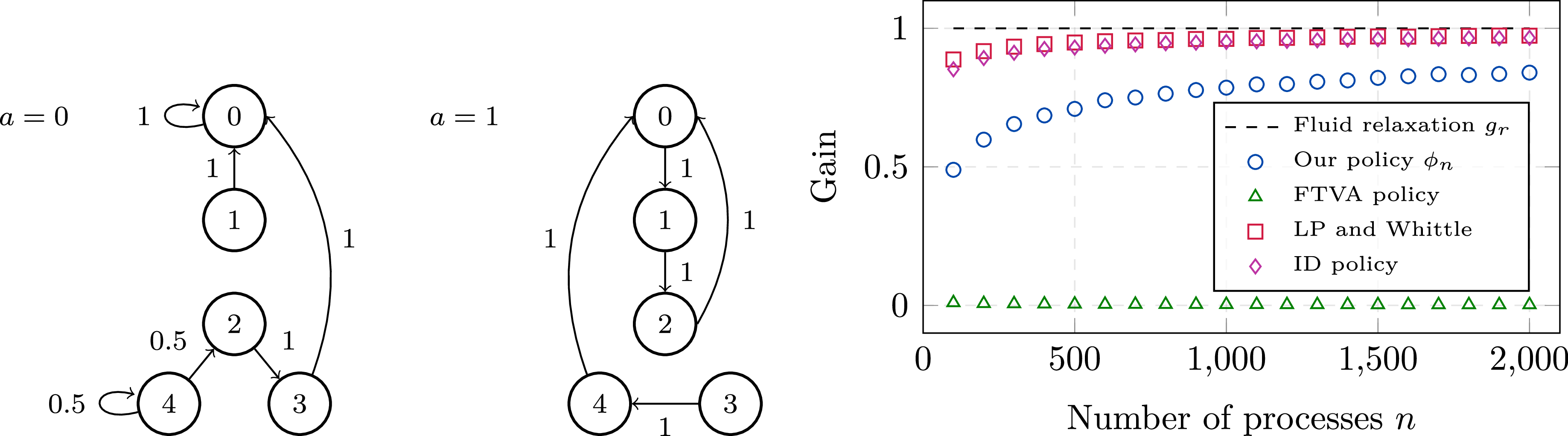
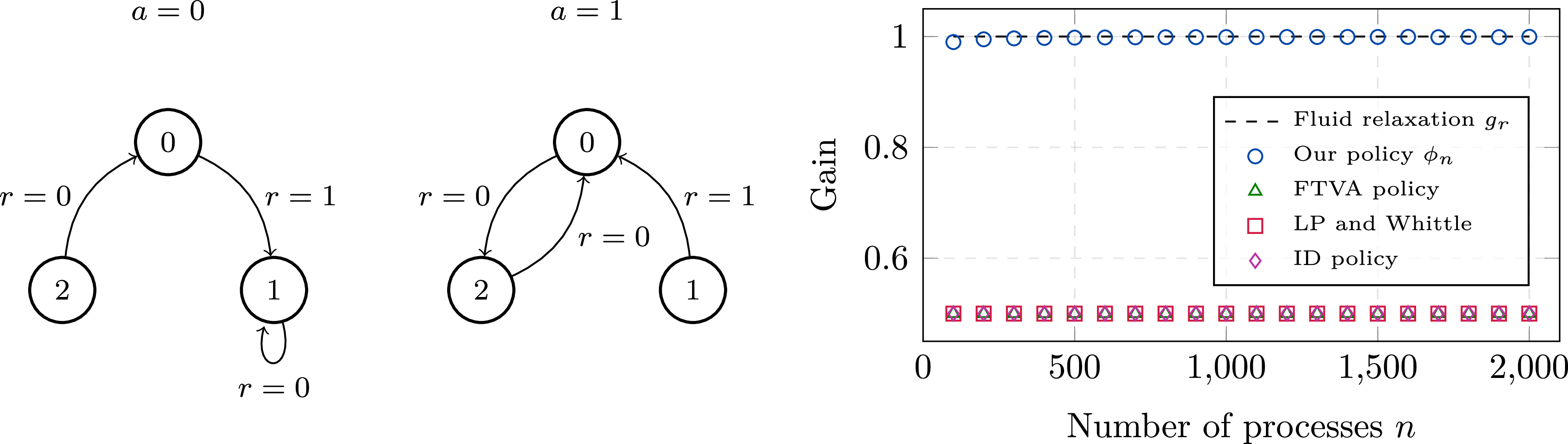
1. Introduction
Consider n identical discrete-time Markov decision processes with finite state and action spaces. Given the states and actions for all the processes, the states reached at the next time step are mutually independent. Nevertheless, the processes are not independent since there exist linear constraints that couple the selection of actions across the processes. The objective is to maximize the expected average reward obtained over an infinite time horizon by selecting the actions in a suitable way that respects the constraints.
The above weakly coupled Markov decision processes can be used to model a wide range of applications, including the healthcare, queueing, supply chain, and scheduling problems considered in [Reference Gocgun and Ghate12, Reference Hawkins14, Reference Meuleau, Hauskrecht, Kim, Peshkin, Kaelbling, Dean and Boutilier19, Reference Patrick, Puterman and Queyranne20, Reference Salemi Parizi22]. The processes typically represent independent agents, projects, or tasks which use shared resources of different types. Selecting an action for a process determines the amount of resources of each type that the process will use over the current time step, as well as the average reward that the process will produce. The constraints can be used to impose conditions on the total amount of each resource that should be used at each time step; e.g. the total amount of resource used may not exceed the amount that is available. For example, suppose that each process represents a taxi in a fleet of electric taxis and the state of the taxi is a discrete battery level. At the start of a shift, each taxi can be charged, deployed to the city center, or deployed to the airport. These are the actions, and there may be constraints on the number of taxis for which the same action can be selected, e.g. the number of charging stations may be smaller than the number of taxis. The expected profit or reward that a taxi will make depends on the action. In particular, charging a taxi incurs a cost and the expected profit for sending a taxi to the city center may not be the same as that for sending the taxi to the airport. We will return to this example in Section 5.
The set of weakly coupled Markov decision processes can be regarded as a single Markov decision process without any constraints, where the constraints are implicitly imposed in the definition of the action space associated with each state. Thus, an optimal policy for the weakly coupled processes can be obtained by leveraging dynamic programming techniques. However, the optimal policy hardly ever admits a closed-form expression, and the time required to compute the policy numerically can often be exceedingly large as it depends exponentially on the number of processes n. This creates a strong incentive for studying simple policies that may not be optimal but become optimal as
 $n \to \infty$
.
While weakly coupled processes have been considered before, the focus has been on problems with finite time horizons or multi-armed restless bandits where only two actions are possible and there is a single constraint with a specific structure. In particular, we are not aware of any previous results for problems with multiple actions and constraints where the goal is to maximize the expected average reward over an infinite time horizon. Our results concern this class of problems and hold under weak assumptions on the transition probability matrices of the processes. These assumptions are provably weaker than those in all previous papers on multi-armed restless bandits, perhaps with the exception of [Reference Hong, Xie, Chen and Wang16]. Although we do not prove that the assumptions in [Reference Hong, Xie, Chen and Wang16] are stronger, we provide examples where our approach yields asymptotically optimal policies and that in [Reference Hong, Xie, Chen and Wang16] does not.
1.1. Overview of the main results
Using standard arguments, we establish that a linear program yields an upper bound for the expected average reward that any policy can provide. Then we prove that a solution of a deterministic and continuous-variable control problem can be used to construct policies for the weakly coupled processes that achieve this upper bound in the limit as
 $n \to \infty$
. We further analyze this fluid problem and derive sufficient conditions for the existence of solutions, as well as structural properties that help to construct a solution.
Under certain assumptions on the constraints of the problem, we show that the conditions are automatically satisfied if the unconstrained single-process problem admits a suitable unichain and aperiodic policy. A Markov chain is unichain if its state space can be partitioned into a single recurrent class and a possibly empty set of transient states; a policy is unichain if the associated Markov chain is unichain, and a Markov decision process is unichain if every stationary deterministic policy is unichain. We note that a unichain and aperiodic policy may exist even if the single-process problem is multichain, i.e. is not unichain. Our assumptions on the constraints include multi-armed restless bandit problems and a broad class of problems with multiple actions and inequality constraints. In both of these cases we provide a simple procedure for constructing asymptotically optimal policies, which we apply to concrete examples and evaluate numerically.
1.1.1. Mean-field limit and asymptotic optimality.
An important characteristic of the weakly coupled processes considered here is that processes in the same state react to the same action in an identically distributed way. In view of this property, we describe the states of all the processes through an occupancy measure or state frequency vector that reflects the empirical distribution of the states. Moreover, we focus our search for asymptotically optimal policies on the class of policies which are defined by mappings that assign to each state frequency vector a state–action frequency vector, i.e. a vector that for each state and action indicates the fraction of processes that are in the given state and for which the given action is selected.
Such a mapping determines a transition kernel that governs the evolution of the state frequency vector as a discrete-time Markov chain. Assuming that the mapping converges uniformly as
 $n \to \infty$
to a continuous function that we call fluid control, we show that the latter stochastic process converges weakly to a nearly deterministic process dubbed fluid trajectory. More precisely, a fluid trajectory has a possibly random initial condition but evolves over time in a deterministic manner, as a discrete-time dynamical system that is governed by the fluid control. The values taken by a fluid trajectory are occupancy measures in a probability simplex, and applying the fluid control to any such measure yields a distribution of state–action pairs which satisfies the constraints of the problem, because the fluid control is the limit of mappings which satisfy the constraints.
The latter mean-field limit connects the weakly coupled Markov decision processes with the above-mentioned fluid problem. Specifically, the fluid problem is to find a continuous fluid control such that the average reward of any fluid trajectory converges to the upper bound provided by the linear program. Assuming that such a fluid control exists, we use an interchange of limits argument to prove that asymptotically optimal policies can be obtained by constructing mappings that converge uniformly to the fluid control.
It follows from this result that the problem of finding asymptotically optimal policies can be decomposed into the following subproblems. First, find a fluid control that solves the fluid problem. Second, construct a discrete approximation of the fluid control for each n. In the case of multi-armed restless bandit problems or the class of problems with multiple actions and inequality constraints mentioned earlier, we establish that the second step can be carried out following a straightforward rounding procedure.
1.1.2. Structure of optimal fluid controls.
In order to find suitable fluid controls, we fix an occupancy measure that solves the linear program and search for continuous fluid controls such that all fluid trajectories converge to this optimal occupancy measure. For this restricted version of the fluid problem, we derive a necessary and sufficient condition for the existence of solutions. The condition involves the set of occupancy measures that assign zero mass to some state in the support of the optimal occupancy measure; this set is contained in the boundary of the simplex. We prove that a solution of the restricted fluid problem exists if and only if there exists a fluid control such that no fluid trajectory is contained in the latter set. Furthermore, we give an explicit expression for a solution using the latter auxiliary fluid control.
Loosely speaking, we solve the restricted fluid problem by expressing every occupancy measure as the sum of two nonnegative measures, such that the first measure is a multiple of the optimal occupancy measure with maximal total mass. The solution of the restricted fluid problem is the fluid control that at each time step keeps the first measure unchanged and applies the auxiliary fluid control to the second measure. The property of the auxiliary fluid control ensures that the first measure absorbs mass from the second measure over time. As a result, all fluid trajectories converge to the optimal occupancy measure.
The global attractivity result reduces the problem of finding an optimal fluid control to that of finding an auxiliary fluid control. For problems with general constraints, we consider auxiliary fluid controls that can be expressed as a convex combination of two other fluid controls. The first one is based on a policy for the unconstrained single-process problem, whereas the purpose of the second one is to ensure that the convex combination complies with the constraints. We prove that the convex combination yields an auxiliary fluid control, with the desired property, if the policy for the unconstrained single-process problem is unichain, aperiodic, and such that the unique irreducible class contains all the states that are in the support of the optimal occupancy measure.
It is difficult to provide an explicit expression for the auxiliary fluid control without imposing some assumptions on the structure of the constraints, because the fluid control must comply with the constraints. We obtain explicit expressions in two important cases: multi-armed restless bandits and a class of problems with multiple actions and inequality constraints. The latter inequality constraints must have nonnegative coefficients, which can be interpreted as amounts of resources that are consumed by the different actions. Also, there must exist an action that does not consume any resources. Applying such an action to a process does not contribute to violating any of the constraints, which makes it easy to obtain feasible policies.
1.2. Related work
As noted earlier, the study of weakly coupled Markov decision processes with multiple actions and constraints has focused on scenarios with finite time horizons. In this context, several papers have studied linear programming and Lagrange decomposition techniques for obtaining approximate solutions and bounds; e.g. [Reference Adelman and Mersereau1, Reference Gocgun and Ghate12, Reference Hawkins14]. Recently, [Reference Brown and Zhang5, Reference Brown and Zhang6, Reference Gast, Gaujal and Yan11] have obtained asymptotic optimality results and performance bounds that depend on the number of processes and the time horizon; here, the formulation in [Reference Brown and Zhang5] allows for exogenous signals that affect the constraints, rewards, and transition probabilities. Similar asymptotic optimality results and performance bounds have been established in the more restrictive scenario where there is a single constraint. In this setting, [Reference Brown and Smith4, Reference Gast, Gaujal and Yan10, Reference Zhang and Frazier29] have considered problems with two actions, whereas [Reference Xiong, Li and Singh26, Reference Zayas-Caban, Jasin and Wang28] have studied problems with more than two actions. It is worth noting that the setups considered in [Reference Brown and Smith4–Reference Brown and Zhang6] allow for heterogeneous processes, as well as time-dependent constraints, rewards, and transition probabilities.
The problems studied in the above papers are substantially different from the ones considered here, where rewards are averaged over an infinite time horizon. In particular, the initial state and the length of the time horizon affect the optimal value and policy of a problem with a finite time horizon. In contrast, the expected average reward over an infinite time horizon is often not affected by the initial state, and the length of the time horizon is meaningless. Further, the structure of the transition kernels plays an important role in problems with the expected average reward criterion but is not particularly relevant when the time horizon is finite. Similar remarks apply to problems with an infinite time horizon and the discounted reward criterion, which can be regarded as problems with a finite but random time horizon. Such problems have been analyzed in [Reference Brown and Smith4, Reference Brown and Zhang6] by truncating the time horizon and applying results for problems with a finite time horizon.
To the best of our knowledge, the expected average reward criterion has only been considered when the processes are coupled by a single constraint. The focus has been on the multi-armed restless bandits introduced by Whittle, which have two actions and a single constraint that fixes the numbers of processes or arms that must select each action. In the seminal paper [Reference Whittle25], Whittle defined an index policy for multi-armed restless bandits where a technical condition known as indexability holds, and conjectured the asymptotic optimality of this policy. A counterexample for this conjecture was provided in [Reference Weber and Weiss24]. However, [Reference Weber and Weiss24] also established that the conjecture is true when a dynamical system defined by the index policy has a global attractor; [Reference Weber and Weiss24] also assumed the ergodicity of the single-arm problem. Exponentially small bounds for the optimality gap were provided in [Reference Gast, Gaujal and Yan9] when the same assumptions hold and the global attractor satisfies a nonsingularity condition. In addition, [Reference Hodge and Glazebrook15] generalized the asymptotic optimality result to multi-armed restless bandit problems with multiple actions and a single constraint with a specific structure.
The Whittle index policy is contained in the class of LP-priority policies introduced in [Reference Verloop23]. The latter paper shows that an LP-priority policy is asymptotically optimal if the problem is unichain and a global attractor assumption holds, while [Reference Gast, Gaujal and Yan10] proves performance bounds. LP-priority policies can be more generally applied than the Whittle index policy since they do not depend on the indexability condition. However, both policies rely on global attractivity assumptions that must be checked for each problem instance; while some of our results also rely on a global attractor property, we formally prove this property instead of assuming that it holds as in [Reference Gast, Gaujal and Yan9, Reference Gast, Gaujal and Yan10, Reference Verloop23, Reference Weber and Weiss24]. More recently, [Reference Hong, Xie, Chen and Wang16, Reference Hong, Xie, Chen and Wang18] have proposed novel policies for multi-armed restless bandits and have established asymptotic optimality results and performance bounds without using the global attractivity assumption.
As observed earlier, our assumptions are provably weaker than those in all of the above papers with the possible exception of [Reference Hong, Xie, Chen and Wang16]. Furthermore, we provide examples where our approach yields asymptotically optimal policies while the above-mentioned policies are not asymptotically optimal, including the one proposed in [Reference Hong, Xie, Chen and Wang16]. We also recall that our approach allows for multiple actions and constraints, while multi-armed restless bandits have only two actions and a single constraint with a specific structure.
Some of the above papers on multi-armed restless bandits have obtained bounds for the optimality gap as a function of the number of arms n. Moreover, some papers have derived bounds that decrease exponentially fast with n by imposing stronger assumptions. Such bounds were first derived in [Reference Gast, Gaujal and Yan9, Reference Gast, Gaujal and Yan10] for the Whittle index and LP-priority policies by requiring, apart from the conditions mentioned earlier, that the solution of a linear program is nondegenerate in a suitable sense. Recently, [Reference Hong, Xie, Chen and Wang17] has proposed a two-set policy with the same performance guarantees under weaker assumptions: the uniform global attractivity property required in [Reference Gast, Gaujal and Yan9, Reference Gast, Gaujal and Yan10] is replaced by a local stability property which is further shown to be necessary for a broad class of problems. The focus of the current paper is not on bounding the optimality gap as a function of the number of processes n, but on obtaining simple policies that are asymptotically optimal under very general assumptions.
At approximately the same time as the conclusion of this work, similar results were derived independently in [Reference Yan27] for the special case of multi-armed restless bandits. The latter paper also uses a deterministic control problem to construct policies that are asymptotically optimal, and the align and steer policy considered in [Reference Yan27] belongs to the class of policies analyzed in the present paper. However, the proof techniques are significantly different. The approach of [Reference Yan27] is motivated by the certainty equivalence control principle of control theory and the proofs are based on the so-called Stein method. In contrast, our approach is motivated by mean-field arguments and our proof techniques combine mean-field limits with interchange of limits and global attractivity arguments. Our results are more general and our approach has the advantage of establishing an explicit connection between the weakly coupled processes and the fluid problem, through mean-field limits.
1.3. Organization of the paper
The rest of the paper is organized as follows. In Section 2 we define the weakly coupled Markov decision processes formally and we discuss standard properties of optimal policies and a linear program relaxation. In Section 3 we prove the mean-field limit and asymptotic optimality results, assuming that a solution of the fluid problem is available. In Section 4 we establish sufficient conditions for the existence of solutions and we obtain structural properties that help to construct a solution. In Section 5 we give concrete examples and evaluate the performance of our policies through numerical experiments. We also compare our policies with policies proposed in the literature on multi-armed restless bandits. In Section 6 we provide some concluding remarks. Some results are proved in Appendix A, and some details about the numerical examples are given in Appendix B.
2. Problem formulation
We consider the problem of maximizing the expected average reward obtained over an infinite time horizon by n identical discrete-time Markov decision processes. Each process has the same finite action space A and state space S. Without loss of generality, we assume that in each state a controller has the same set of actions. Given the states and actions for all the processes, the states reached at the next time step are mutually independent, and the probability that a process moves to state j given that it is in state i and action a is selected for it is denoted by
 $p(j \mid i, a)$
. However, the processes are not independent since there exist linear constraints that couple the selection of actions across the processes.
The action and state of process
 $m \in \{1, \ldots, n\}$
at time
 $t \in \mathbb{N}$
are the random variables denoted by
 ${\boldsymbol{{A}}}_n(t, m)$
and
 ${\boldsymbol{{S}}}_n(t, m)$
, respectively; throughout the paper we use boldface notation for quantities that depend on time. We further define
 \begin{equation} {\boldsymbol{{x}}}_n(t, i) \,:\!=\, \frac{1}{n}\sum_{m = 1}^n \mathbf{1}_{\{{\boldsymbol{{S}}}_n(t, m) = i\}}, \qquad \quad {\boldsymbol{{y}}}_n(t, i, a) \,:\!=\, \frac{1}{n}\sum_{m = 1}^n \mathbf{1}_{\{{\boldsymbol{{S}}}_n(t, m) = i, {\boldsymbol{{A}}}_n(t, m) = a\}}\end{equation}
for all
 $t \in \mathbb{N}$
,
 $i \in S$
, and
 $a \in A$
. For each time t, the fraction of processes in state i is given by the former quantity, while the latter quantity represents the fraction of processes that are in state i for which action a is selected. In particular,
 ${\boldsymbol{{x}}}_n(t) \in \mathbb{R}^S$
and
 ${\boldsymbol{{y}}}_n(t) \in \mathbb{R}^{S \times A}$
are vectors describing the state and state–action frequencies at time t, respectively.
Suppose that we have p equality constraints and q inequality constraints, and consider matrices
 $\{C_n(a) \colon a \in A\}$
and
 $\{E_n(a) \colon a \in A\}$
with rows indexed by
 $i \in S$
such that the former matrices have p columns and the latter matrices have q columns. Further, let
 $d_n$
and
 $f_n$
be row vectors with p and q entries, respectively. The processes are weakly coupled by the following constraints:
 \begin{align} &\sum_{a \in A} {\boldsymbol{{y}}}_n(t, a) C_n(a) = d_n \quad \text{for all} \ t \in \mathbb{N}, \\[-12pt] \nonumber \end{align}
 \begin{align} &\sum_{a \in A} {\boldsymbol{{y}}}_n(t, a) E_n(a) \preceq f_n \quad \text{for all} \ t \in \mathbb{N}. \\[6pt] \nonumber \end{align}
In the above expressions
 ${\boldsymbol{{y}}}_n(t, a) \,:\!=\, ({\boldsymbol{{y}}}_n(t, i, a) \colon i \in S)$
represents a row vector, and the notation
 $\preceq$
in the second line refers to componentwise inequality.
At each time, a reward r(i, a) is obtained by each process in state i for which action a is selected. Informally speaking, we must select the actions over time to maximize
 \begin{equation} \lim_{T \to \infty} \frac{1}{T}\sum_{t = 0}^{T - 1} \frac{1}{n}\sum_{m = 1}^n \mathbb{E}[r({\boldsymbol{{S}}}_n(t, m), {\boldsymbol{{A}}}_n(t, m))] = \lim_{T \to \infty} \frac{1}{T}\sum_{t = 0}^{T - 1} \sum_{a \in A} \mathbb{E}[{\boldsymbol{{y}}}_n(t, a)]r(a)\end{equation}
while complying with the constraints (2); the objective will be formally stated in the next section, where the existence of the limits is addressed. The expression on the left is called gain and represents the expected reward per unit of time obtained by one process, averaged across all the processes and over time. On the right,
 $r(a) \,:\!=\, (r(i, a) \colon i \in S)$
is a column vector, and the equality follows from the definition of the state–action frequencies.
For example, the processes could represent projects that are carried out in parallel and produce revenues or expenses over time; the latter correspond to negative rewards. The goal is to provide a policy for selecting the actions over time in a way that maximizes the average profit obtained per unit of time in the long run. If the matrices and vectors in (2) are nonnegative, then the relations in (2) can be interpreted as constraints in the allocation of
 $p + q$
resources. Namely, performing action a when a project is in state i involves
 $C_n(i, k, a)$
units of resource
 $k \in \{1, \ldots, p\}$
and
 $E_n(i, l, a)$
units of resource
 $p + l \in \{p + 1, \ldots, p + q\}$
. For instance, suppose that these resources are employees and trucks, respectively. Then there are
 $n d_n(k)$
employees and
 $n f_n(l)$
trucks in total. Also, (2a) says that all the employees must work in some project and (2b) says that it is not necessary to use all the trucks.
If
 $A = \{0, 1\}$
and one of the following conditions holds, then the set of weakly coupled Markov decision processes is called a multi-armed restless bandit.
-
(i) There is a unique equality constraint and there are no inequality constraints. Also, the unique equality constraint satisfies
 $n d_n \in \{1, \ldots, n\}$
while
$C_n(i, 0) = 0$
and
$C_n(i, 1) = 1$
for all
$i \in S$
.
-
(ii) There is a unique inequality constraint and there are no equality constraints. Further, the unique inequality constraint satisfies
$f_n \in [0, 1]$
while
$E_n(i, 0) = 0$
and
$E_n(i, 1) = 1$
for all
$i \in S$
.



In the above expressions,
 $d_n$
and
 $f_n$
are scalars, and
 $C_n(a)$
and
 $E_n(a)$
are column vectors for each
 $a \in A$
. As noted in Section 1, multi-armed restless bandit problems have received considerable attention, under either of the latter conditions. The setup consider in the present paper is significantly more general.
2.1. Existence of optimal policies
The weakly coupled processes can be regarded as a single Markov decision process with finite state and action spaces. Specifically, the state space is
 $S^n$
and the action space for a given state is the subset of
 $A^n$
where the coupling constraints (2) hold. More precisely, a state
 $(i_1, \ldots, i_n) \in S^n$
and a tuple
 $(a_1, \ldots, a_n) \in A^n$
uniquely determine a vector y of state–action frequencies as in (1). The action space at a given state
 $(i_1, \ldots, i_n)$
is the subset of
 $A^n$
such that the state–action frequency vector y satisfies (2).
Consider the sets
 $\Pi_n^\mathrm{SD} \subset \Pi_n^\mathrm{SR} \subset \Pi_n^\mathrm{HR}$
of stationary and deterministic, stationary and randomized, and history-dependent and randomized policies for the latter Markov decision process; see [Reference Puterman21, Section 2.1.5] for precise definitions. Loosely speaking, stationary policies select actions using solely the current state, whereas the history-dependent policies select actions using the current state and the history of all past states and actions. Randomized policies can be regarded as mappings that assign to each state, or history of states and actions, a probability distribution defined over the action space of the current state; an action is then sampled from this distribution. The policy is called deterministic if the latter probability distribution is always concentrated at a single action.
It follows from [Reference Puterman21, Proposition 8.1.1] that the gain
 \begin{equation*} g_n^\pi(s) \,:\!=\, \lim_{T \to \infty} \frac{1}{T}\sum_{t = 0}^{T - 1} \frac{1}{n}\sum_{m = 1}^n \mathbb{E}_s^\pi[r({\boldsymbol{{S}}}_n(t, m), {\boldsymbol{{A}}}_n(t, m))] = \lim_{T \to \infty} \frac{1}{T}\sum_{t = 0}^{T - 1} \sum_{a \in A} \mathbb{E}_s^\pi[{\boldsymbol{{y}}}_n(t, a)]r(a)\end{equation*}
exists for all policies
 $\pi \in \Pi_n^\mathrm{SR}$
and initial states
 $s \in S^n$
, i.e. the limits in (3) exist. Here, the expectation is taken with respect to the Markov chain defined by the initial state and the stationary and randomized policy. Also, [Reference Puterman21, Theorems 9.1.7 and 9.1.8] imply that
 \begin{equation*} g_n^*(s) \,:\!=\, \sup\nolimits_{\pi \in \Pi_n^\mathrm{SD}} g_n^\pi(s)\end{equation*}
is attained simultaneously for all
 $s \in S^n$
by some
 $\pi^* \in \Pi_n^\mathrm{SD}$
, and [Reference Puterman21, Theorem 9.1.6] yields
 \begin{equation*} g_n^*(s) = \sup_{\pi \in \Pi_n^\mathrm{HR}} \limsup_{T \to \infty} \frac{1}{T}\sum_{t = 0}^{T - 1} \frac{1}{n}\sum_{m = 1}^n \mathbb{E}_s^\pi[r({\boldsymbol{{S}}}_n(t, m), {\boldsymbol{{A}}}_n(t, m))].\end{equation*}
In other words, there exists a stationary and deterministic policy
 $\pi^*$
that has maximal gain across all the initial states. This policy maximizes the expressions in (3) over the set of policies for which the limits exist, and provides an expected average reward not smaller than any history-dependent and randomized policy, as stated in the previous equation.
An optimal policy
 $\pi^*$
does not typically admit a closed-form expression. While
 $\pi^*$
can be computed numerically using dynamic programming, the computation time is exponential in the number of processes n and thus exceedingly large in many applications. This creates an incentive for simple policies that perform well when n is large.
2.2. Fluid relaxation
In this paper we analyze a class of policies that are easy to compute and asymptotically optimal, i.e. they achieve the maximum gain as
 $n \to \infty$
. For this purpose we adopt the following assumption throughout the paper. It says that (2) is consistent in the limit.
Assumption 1. For each
 $a \in A$
, the following limits exist and are finite:
 \begin{equation*} C(a) \,:\!=\, \lim_{n \to \infty} C_n(a), \qquad d \,:\!=\, \lim_{n \to \infty} d_n, \qquad E(a) \,:\!=\, \lim_{n \to \infty} E_n(a), \qquad f \,:\!=\, \lim_{n \to \infty} f_n. \end{equation*}
Let
 $e \in \mathbb{R}^S$
denote the column vector with each of its entries equal to one. The processes of state and state–action frequencies
 ${\boldsymbol{{x}}}_n$
and
 ${\boldsymbol{{y}}}_n$
take values in
 \begin{equation*} X \,:\!=\, \{x \in [0, 1]^{S} \colon x e = 1\}, \qquad Y \,:\!=\, \Bigg\{y \in [0, 1]^{S \times A} \colon \sum_{a \in A} y(a)e = 1\Bigg\},\end{equation*}
respectively; x and
 $y(a) = (y(i, a) \colon i \in S)$
are regarded as row vectors. For each
 $a \in A$
, let P(a) denote the matrix such that the entry (i, j) is
 $p(j \mid i, a)$
. The following linear program will play an important role throughout the paper.
Definition 1. We call fluid relaxation the following optimization problem:
 \begin{align} & \underset{y \in Y}{\text{maximize}} \quad \sum_{a \in A} y(a)r(a) \nonumber\\ & \text{subject to} \quad \sum_{a \in A} y(a)P(a) = \sum_{a \in A} y(a), \sum_{a \in A} y(a)C(a) = d, \qquad \sum_{a \in A} y(a)E(a) \preceq f. \end{align}
Its optimal value is denoted by
 $g_r$
.
The optimization variables y(i, a) can be interpreted as
 \begin{equation*} \lim_{n \to \infty} \lim_{T \to \infty} \frac{1}{T}\sum_{t = 0}^{T - 1} \mathbb{E}[{\boldsymbol{{y}}}_n(t, i, a)]\end{equation*}
when the limits exist. The first constraint in (4) is a balance equation that is satisfied by long-run averages as defined by the inner limit; see the proof of the next proposition. The other constraints say that these long-run averages must satisfy (2) as
 $n \to \infty$
. Moreover, the objective of the problem can be interpreted as the limiting gain.
The following proposition says that
 $g_r$
is an upper bound for the gain of the weakly coupled Markov decision processes as
 $n \to \infty$
. An intuitive explanation of this result, based on the above interpretation of (4), is that the constraints (2) must hold at each time and for each sample path, whereas the constraints of (4) are only imposed on long-run averages, thereby relaxing the problem. The proof of the proposition is standard but we provide it in Appendix A for completeness.
Proposition 1. For each
 $a \in A$
and some fixed n, suppose that
 \begin{equation} C_n(a) = C(a), \qquad d_n = d, \qquad E_n(a) = E(a), \qquad f_n = f. \end{equation}
Then
 $g_n^*(s) \leq g_r$
for all
 $s \in S^n$
. In the general case where (5) may not hold, we have
 \begin{equation} \limsup_{n \to \infty} \sup\nolimits_{s \in S^n} g_n^*(s) \leq g_r. \end{equation}
In the following two sections we will establish that the inequality in (6) is in fact an equality under mild assumptions. Moreover, we will provide stationary policies for the n weakly coupled processes with gains that approach
 $g_r$
as
 $n \to \infty$
.
3. Asymptotic optimality
An important characteristic of the weakly coupled processes is that two processes in the same state will react to the same action in an identically distributed way. Therefore, it makes sense to focus the search for asymptotically optimal policies on a class of policies that do not distinguish between two processes that are in the same state. More precisely, we may restrict our attention to stationary policies which can be defined by mappings that assign to each state frequency vector a state–action frequency vector. Mean-field theory suggests that then the state and state–action frequency processes
 ${\boldsymbol{{x}}}_n$
and
 ${\boldsymbol{{y}}}_n$
behave deterministically in the limit as
 $n \to \infty$
, which motivates the next definition.
Definition 2. Consider a function
 $\phi \colon X \longrightarrow Y$
and let us use the short-hand notation
 $\phi(x, a)$
for
 $y(a)$
when
 $y = \phi(x)$
. The latter function is called a fluid control if
 $\sum_{a \in A} \phi(x, a) = x$
,
 $\sum_{a \in A} \phi(x, a)C(a) = d$
, and
 $\sum_{a \in A} \phi(x, a)E(a) \preceq f$
for all
 $x \in X$
. The fluid trajectory induced by a fluid control
 $\phi$
and an initial condition
 $x^0 \in X$
is the sequence
 $\{{\boldsymbol{{x}}}(t), {\boldsymbol{{y}}}(t) \colon t \in \mathbb{N}\}$
defined recursively by
 ${\boldsymbol{{x}}}(0) = x^0$
,
 ${\boldsymbol{{y}}}(t) = \phi({\boldsymbol{{x}}}(t))$
, and
 ${\boldsymbol{{x}}}(t + 1) = \sum_{a \in A} {\boldsymbol{{y}}}(t, a)P(a)$
for all
 $t \geq 0$
.
The deterministic vectors
 ${\boldsymbol{{x}}}(t)$
and
 ${\boldsymbol{{y}}}(t)$
can be regarded as the fluid counterparts of
 ${\boldsymbol{{x}}}_n(t)$
and
 ${\boldsymbol{{y}}}_n(t)$
, respectively, while
 $\phi$
is the counterpart of a policy that assigns to each state frequency vector x a state–action frequency vector
 $\phi(x)$
. The first condition imposed on
 $\phi$
is that the state–action frequencies must be consistent with the state frequencies, whereas the other two conditions enforce the constraints (2), with the matrices and vectors therein replaced by the limits in Assumption 1. The dynamics defining a fluid trajectory state that the fluid control
 $\phi$
determines the state–action frequencies
 ${\boldsymbol{{y}}}(t)$
as a function of the state frequencies
 ${\boldsymbol{{x}}}(t)$
, and then
 ${\boldsymbol{{x}}}(t + 1)$
is obtained analogously to
 $\mathbb{E}[{\boldsymbol{{x}}}_n(t + 1)] = \sum_{a \in A} \mathbb{E}[{\boldsymbol{{y}}}_n(t, a)]P(a)$
. This equation holds for the n processes and any given policy, provided that the expectations are conditional on the policy and the initial states of all the processes.
Note that
 ${\boldsymbol{{x}}}_n$
and
 ${\boldsymbol{{y}}}_n$
take values in the discrete spaces
 $X_n \,:\!=\, \{x \in X \colon nx \in \mathbb{Z}^S\}$
and
 $Y_n \,:\!=\, \{y \in Y \colon ny \in \mathbb{Z}^{S \times A}\}$
, respectively. In general, a fluid control may not define a policy for the n weakly coupled processes because its values may be outside of
 $Y_n$
or not satisfy (2). However, a principled way of obtaining policies that do not distinguish between processes in the same state is to first search for a fluid control
 $\phi \colon X \longrightarrow Y$
and then construct functions
 $\phi_n \colon X_n \longrightarrow Y_n$
that resemble
 $\phi$
and define admissible policies for the n processes.
Definition 3. Consider functions
 $\phi_n \colon X_n \longrightarrow Y_n$
and let us use the short-hand notation
 $\phi_n(x, a)$
for
 $y(a)$
when
 $\phi_n(x) = y$
, as for fluid controls. Also, assume that
 $\sum_{a \in A} \phi_n(x, a) = x$
,
 $\sum_{a \in A} \phi_n(x, a)C_n(a) = d_n$
, and
 $\sum_{a \in A} \phi_n(x, a)E_n(a) \preceq f_n$
if
 $x \in X_n$
. The functions
 $\{\phi_n \colon n \geq 1\}$
are discrete controls associated with a fluid control
 $\phi$
if
 $\lim_{n \to \infty} \max_{x \in X_n} ||\phi(x) - \phi_n(x)|| = 0$
; the norm
 $||{\cdot}||$
can be arbitrary.
The mapping
 $\phi_n$
assigns to each
 $x \in X_n$
a state–action frequency vector
 $\phi_n(x) \in Y_n$
that satisfies the constraints (2). We say that a policy
 $\pi \in \Pi_n^\mathrm{SR}$
realizes
 $\phi_n$
if
 ${\boldsymbol{{y}}}_n(t) = \phi_n({\boldsymbol{{x}}}_n(t))$
for all
 $t \geq 0$
when
 $\pi$
is used. A policy that realizes
 $\phi_n$
can be obtained by computing
 ${\boldsymbol{{y}}}_n(t)$
as above and then selecting the
 $n {\boldsymbol{{y}}}_n(t, i, a)$
processes that use action a in state i uniformly at random among all the processes in state i. While a policy that realizes
 $\phi_n$
is generally not unique, the gain and the joint law of the processes
 ${\boldsymbol{{x}}}_n$
and
 ${\boldsymbol{{y}}}_n$
are the same for any such policy; they are determined by
 $\phi_n$
and the initial state frequencies. Hence, we will focus on the mappings
 $\phi_n$
without specifying the policies that realize these mappings explicitly.
Later on in this section we will assume that a fluid control
 $\phi$
is available, and that
 $\phi$
is a continuous function such that every fluid trajectory satisfies
 \begin{equation} \lim_{t \to \infty} \sum_{a \in A} {\boldsymbol{{y}}}(t, a) r(a) = g_r,\end{equation}
regardless of the initial condition. Using mean-field arguments, we will prove that the gain of any discrete control
 $\phi_n$
associated with
 $\phi$
approaches
 $g_r$
as
 $n \to \infty$
; we will not require any conditions on the discrete controls besides those already stated in Definition 3.
In view of the latter result, the problem of finding asymptotically optimal policies can be decomposed into the following two subproblems:
-
(i) Fluid problem: Construct a continuous fluid control
$\phi$
that satisfies (7). -
(ii) Approximation problem: Construct discrete controls
$\phi_n$
as in Definition 3.


Section 4 will focus on (i), which is the harder problem. Then the discrete controls in (ii) can be defined by letting
 $\phi_n(x)$
be the solution of the following optimization problem:
 \begin{align*} & \underset{y \in Y_n}{\text{minimize}} \quad ||y - \phi(x)|| \\ & \text{subject to} \quad \sum_{a \in A} y(a) = x, \qquad \sum_{a \in A} y(a)C_n(a) = d_n, \qquad \sum_{a \in A} y(a)E_n(a) \preceq f_n. \end{align*}
However, simpler rounding procedures are possible under certain conditions; two such procedures and the corresponding conditions are discussed in Section 4. A final step would be to define policies
 $\pi_n$
that realize the discrete controls
 $\phi_n$
, but this is straightforward; e.g. it can be done through the random sampling procedure mentioned earlier.
3.1. Mean-field limit
Consider discrete controls
 $\phi_n$
associated with a fluid control
 $\phi$
. As observed earlier, the joint distribution of the state and state–action frequency processes associated with any policy that realizes
 $\phi_n$
is completely determined by
 $\phi_n$
and the initial state frequencies. Further,
 ${\boldsymbol{{x}}}_n$
is a discrete-time Markov chain and
 ${\boldsymbol{{y}}}_n(t) = \phi_n({\boldsymbol{{x}}}_n(t))$
for all
 $t \geq 0$
. Below we provide a convenient construction of these two processes.
For this purpose we consider a collection
 $\{B_t^l(j \mid i, a) \colon l \geq 1,\, t \geq 1,\, i, j \in S,\, a \in A\}$
of Bernoulli random variables with the following two properties. First,
 $B_t^l(j \mid i, a) = 1$
and
 $B_t^l(k \mid i, a) = 0$
for all
 $k \neq j$
with probability
 $p(j \mid i, a)$
for all
 $l \geq 1$
,
 $t \geq 1$
,
 $i \in S$
, and
 $a \in A$
. Second, the random vectors
 $(B_t^l(j \mid i, a) \colon j \in S)$
are independent across
 $l \geq 1$
,
 $t \geq 1$
,
 $i \in S$
, and
 $a \in A$
. The same collection of random variables can be used to construct the state and state–action frequency processes for any given n, and thus the notation does not account for the number of processes n.
At each time t, there are
 $n{\boldsymbol{{y}}}_n(t, i, a)$
processes in state i with action a selected, which we arrange according to their indexes. We postulate that the process with the lth largest index is in state j at
 $t + 1$
if
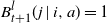 $B_{t + 1}^l(j \mid i, a) = 1$
, which endows
 ${\boldsymbol{{x}}}_n(t + 1)$
with the desired distribution. More specifically, we construct
 ${\boldsymbol{{x}}}_n$
and
 ${\boldsymbol{{y}}}_n$
recursively as functions of
 ${\boldsymbol{{x}}}_n(0)$
and the above Bernoulli random variables such that, for each
 $t \geq 0$
,
 \begin{equation*} {\boldsymbol{{y}}}_n(t) = \phi_n({\boldsymbol{{x}}}_n(t)), \qquad {\boldsymbol{{x}}}_n(t + 1, j) = \frac{1}{n}\sum_{i \in S} \sum_{a \in A} \sum_{l = 1}^{n{\boldsymbol{{y}}}_n(t, i, a)} B_{t + 1}^l(j \mid i, a) \quad \text{for all} \ j \in S.\end{equation*}
We further define
 \begin{equation*} {\boldsymbol{{z}}}_n(t + 1, j) \,:\!=\, \frac{1}{n}\sum_{i \in S} \sum_{a \in A} \sum_{l = 1}^{n{\boldsymbol{{y}}}_n(t, i, a)} \big[B_{t + 1}^l(j \mid i, a) - p(j \mid i, a) \big]\end{equation*}
for all
 $t \geq 0$
and
 $j \in S$
. Then we can write
 \begin{equation} {\boldsymbol{{x}}}_n(t + 1) = {\boldsymbol{{z}}}_n(t + 1) + \sum_{a \in A} {\boldsymbol{{y}}}_n(t, a)P(a) \quad \text{for all} \ t \geq 0.\end{equation}
Clearly,
 ${\boldsymbol{{z}}}_n(t)$
has mean zero for all
 $t \geq 1$
; it is possible to check that
 ${\boldsymbol{{z}}}_n$
is in fact a martingale difference with respect to the natural filtration, but this will not be used explicitly. The next lemma bounds the variance of
 ${\boldsymbol{{z}}}_n(t)$
and is proved in Appendix A.
Lemma 1. Consider the constants
 \begin{equation*} q_{\min}(j) \,:\!=\, \min_{i \in S, a \in A}[1 - p(j \mid i, a)] \leq \max_{i \in S, a \in A}[1 - p(j \mid i, a)] =: q_{\max}(j) \quad \text{for all} \ j \in S. \end{equation*}
For each
 $t \geq 1$
and
 $j \in S$
, we have
 \begin{equation*} \frac{q_{\min}(j)}{n}\mathbb{E}[{\boldsymbol{{x}}}_n(t, j)] \leq \mathbb{E}\big[{\boldsymbol{{z}}}_n^2(t, j)\big] \leq \frac{q_{\max}(j)}{n}\mathbb{E}[{\boldsymbol{{x}}}_n(t, j)]. \end{equation*}
The lemma will be used in the proof of the following proposition, which establishes that the fluid trajectories defined by the fluid control
 $\phi$
are the mean-field limit of the state and state–action frequency processes
 ${\boldsymbol{{x}}}_n$
and
 ${\boldsymbol{{y}}}_n$
determined by
 $\phi_n$
. More precisely, the latter processes converge weakly to fluid trajectories provided that the initial state frequency vectors
 ${\boldsymbol{{x}}}_n(0)$
have a limit in distribution as
 $n \to \infty$
.
Proposition 2. Assume that
 $\phi$
is continuous, and that there exists a random variable
 $x^0$
with values in X such that
 ${\boldsymbol{{x}}}_n(0) \Rightarrow x^0$
as
 $n \to \infty$
. Furthermore, suppose that
 $x^0$
is defined on some set
 $\Omega$
, and for each
 $\omega \in \Omega$
let
 $\{{\boldsymbol{{x}}}(\omega, t), {\boldsymbol{{y}}}(\omega, t) \colon \geq 0\}$
be the fluid trajectory with
 ${\boldsymbol{{x}}}(\omega, 0) = x^0(\omega)$
, which defines two stochastic processes. Then
 ${\boldsymbol{{x}}}_n(t) \Rightarrow {\boldsymbol{{x}}}(t)$
and
 ${\boldsymbol{{y}}}_n(t) \Rightarrow {\boldsymbol{{y}}}(t)$
as
 $n \to \infty$
for all
 $t \geq 0$
.
Proof. We proceed by induction, assuming that
 ${\boldsymbol{{x}}}_n(t) \Rightarrow {\boldsymbol{{x}}}(t)$
as
 $n \to \infty$
and then showing that
 ${\boldsymbol{{y}}}_n(t) \Rightarrow {\boldsymbol{{y}}}(t)$
and
 ${\boldsymbol{{x}}}_n(t + 1) \Rightarrow {\boldsymbol{{x}}}(t + 1)$
. Clearly, the assumption holds for
 $t = 0$
.
Assume that
 ${\boldsymbol{{x}}}_n(t) \Rightarrow {\boldsymbol{{x}}}(t)$
as
 $n \to \infty$
and let
 $\zeta \colon \mathbb{R}^{S \times A} \times X \longrightarrow \mathbb{R}^{S \times A}$
be defined by
 $\zeta(w, x) \,:\!=\, w + \phi(x)$
. If we let
 ${\boldsymbol{{w}}}_n(t) \,:\!=\, \phi_n({\boldsymbol{{x}}}_n(t)) - \phi({\boldsymbol{{x}}}_n(t))$
, then
 ${\boldsymbol{{y}}}_n(t) = \zeta({\boldsymbol{{w}}}_n(t), {\boldsymbol{{x}}}_n(t))$
. Moreover,
 ${\boldsymbol{{w}}}_n(t) \Rightarrow 0$
as
 $n \to \infty$
by Definition 3, because
 $||{\boldsymbol{{w}}}_n(t)|| \leq \max_{x \in X_n}||\phi_n(x) - \phi(x)||$
. By [Reference Billingsley3, Theorem 3.1], we have
 $({\boldsymbol{{w}}}_n(t), {\boldsymbol{{x}}}_n(t)) \Rightarrow (0, {\boldsymbol{{x}}}(t))$
as
 $n \to \infty$
; see [Reference Goldsztajn, Borst and Van Leeuwaarden13, Lemma 9] for further details. The continuous mapping theorem yields
 ${\boldsymbol{{y}}}_n(t) \Rightarrow \zeta(0, {\boldsymbol{{x}}}(t)) = {\boldsymbol{{y}}}(t)$
.
Lemma 1 implies that
 ${\boldsymbol{{z}}}_n(t + 1) \Rightarrow 0$
as
 $n \to \infty$
since
 \begin{equation*} \mathbb{P}\big(||{\boldsymbol{{z}}}_n(t + 1)||_2^2 \geq \varepsilon\big) \leq \frac{\mathbb{E}\big[||{\boldsymbol{{z}}}_n(t + 1)||_2^2 \big]}{\varepsilon} \leq \frac{\mathbb{E}[||{\boldsymbol{{x}}}_n(t)||_1]}{n\varepsilon} \leq \frac{1}{n\varepsilon} \quad \text{for all} \ \varepsilon > 0. \end{equation*}
Therefore,
 $({\boldsymbol{{y}}}_n(t), {\boldsymbol{{z}}}_n(t + 1)) \Rightarrow ({\boldsymbol{{y}}}(t), 0)$
as
 $n \to \infty$
by [Reference Billingsley3, Theorem 3.1]. Consider now the continuous function
 $\eta \colon \mathbb{R}^{S \times A} \times \mathbb{R}^S \longrightarrow \mathbb{R}^S$
such that
 $\eta(y, z) \,:\!=\, z + \sum_{a \in A} y(a)P(a)$
. Then
 ${\boldsymbol{{x}}}_n(t + 1) = \eta({\boldsymbol{{y}}}_n(t), {\boldsymbol{{z}}}_n(t + 1))$
by (8), and it follows from the continuous mapping theorem that
 ${\boldsymbol{{x}}}_n(t + 1) \Rightarrow \eta({\boldsymbol{{y}}}(t), 0) = {\boldsymbol{{x}}}(t + 1)$
as
 $n \to \infty$
.
3.2. Asymptotic optimality result
The next lemma assumes that the fluid control
 $\phi$
is continuous and satisfies (7). Under these assumptions, the lemma establishes that the gain achieved by the discrete control
 $\phi_n$
approaches the optimal value of the fluid relaxation
 $g_r$
as
 $n \to \infty$
whenever
 ${\boldsymbol{{x}}}_n(0)$
has a stationary distribution for each n; at least one stationary distribution for the Markov chain
 ${\boldsymbol{{x}}}_n$
always exists since its state space is finite, but this distribution may not be unique. The proof of the lemma relies on the mean-field limit obtained in Proposition 2.
Lemma 2. Assume that
 $\phi$
is continuous and that every fluid trajectory satisfies
 \begin{equation*} \lim_{t \to \infty} \sum_{a \in A} {\boldsymbol{{y}}}(t, a) r(a) = g_r, \end{equation*}
regardless of the initial condition. Also, assume that
 ${\boldsymbol{{x}}}_n(0)$
is distributed as a stationary distribution of
 ${\boldsymbol{{x}}}_n$
, and thus
 ${\boldsymbol{{x}}}_n$
is stationary. Then
 \begin{equation} \lim_{n \to \infty}\sum_{a \in A}\mathbb{E}[{\boldsymbol{{y}}}_n(t, a)]r(a) = g_r \quad \text{for all} \ t \geq 0. \end{equation}
Proof. Consider the following limits in distribution:
 \begin{equation} \sum_{a \in A} {\boldsymbol{{y}}}_n(t, a)r(a) \Rightarrow g_r \quad \text{as} \ n \to \infty \ \text{for all} \ t \geq 0. \end{equation}
For each
 $t \geq 0$
, the sequence of random variables on the left-hand side, with t fixed and n varying, is uniformly integrable since it is uniformly bounded:
 \begin{equation} \Bigg|\sum_{a \in A}{\boldsymbol{{y}}}_n(t, a)r(a)\Bigg| \leq |S| |A| \max_{i \in S, a \in A} |r(i, a)|. \end{equation}
We conclude that (10) implies (9), so it suffices to prove (10). Because
 ${\boldsymbol{{x}}}_n$
is stationary, the following random variables are identically distributed:
 \begin{equation*} \sum_{a \in A} {\boldsymbol{{y}}}_n(t, a)r(a) = \sum_{a \in A} \phi_n({\boldsymbol{{x}}}_n(t), a)r(a) \sim \sum_{a \in A} \phi_n({\boldsymbol{{x}}}_n(0), a)r(a) = \sum_{a \in A} {\boldsymbol{{y}}}_n(0, a)r(a). \end{equation*}
Hence, it is enough to prove that (10) holds for
 $t = 0$
.
It follows from (11) that
 $\big\{\sum_{a \in A} {\boldsymbol{{y}}}_n(0, a)r(a) \colon n \geq 1\big\}$
is tight, and thus every subsequence has a further subsequence that converges weakly. We will establish (10) for
 $t = 0$
by showing that the weak limit of every convergent subsequence is
 $g_r$
, i.e. the random variable equal to
 $g_r$
with probability 1.
Suppose that
 $\mathcal{L} \subset \mathbb{N}$
and
 $g_{\mathcal{L}}$
are such that
 \begin{equation} \sum_{a \in A} {\boldsymbol{{y}}}_l(0, a)r(a) \Rightarrow g_{\mathcal{L}} \quad \text{as} \ l \to \infty \ \text{while} \ l \in \mathcal{L}. \end{equation}
More specifically,
 $g_{\mathcal{L}}$
is the limit associated with the convergent subsequence indexed by
 $\mathcal{L}$
, and the subscript indicates that this limit could in principle depend on the specific set of indexes
 $\mathcal{L}$
. The random variables
 $\{{\boldsymbol{{x}}}_l(0) \colon l \in \mathcal{L}\}$
are tight because they are all supported on the compact set X. Therefore, we may assume without any loss of generality that there exists a random variable
 $x_{\mathcal{L}}$
such that
 ${\boldsymbol{{x}}}_l(0) \Rightarrow x_{\mathcal{L}}$
as
 $l \to \infty$
.
Define
 $\xi \colon \mathbb{R} \times \mathbb{R}^S \longrightarrow \mathbb{R}$
by
 $\xi(w, x) \,:\!=\, w + \sum_{a \in A} \phi(x, a)r(a)$
. Note that
 $\xi$
is a continuous function and satisfies
 \begin{equation*} \sum_{a \in A} {\boldsymbol{{y}}}_l(0, a)r(a) = \xi\Bigg(\sum_{a \in A}\phi_l({\boldsymbol{{x}}}_l(0), a)r(a) - \sum_{a \in A}\phi({\boldsymbol{{x}}}_l(0), a)r(a), {\boldsymbol{{x}}}_l(0)\Bigg). \end{equation*}
The first argument of
 $\xi$
converges to zero in probability as
 $l \to \infty$
by Definition 3, because
 \begin{equation*} \Bigg|\sum_{a \in A}\phi_l({\boldsymbol{{x}}}_l(0), a)r(a) - \sum_{a \in A}\phi({\boldsymbol{{x}}}_l(0), a)r(a)\Bigg| \leq \max_{x \in X_l}||\phi_l(x) - \phi(x)||\sum_{a \in A}||r(a)||. \end{equation*}
It follows from [Reference Billingsley3, Theorem 3.1] and the continuous mapping theorem that
 \begin{equation*} \sum_{a \in A} {\boldsymbol{{y}}}_l(0, a)r(a) \Rightarrow \xi(0, x_{\mathcal{L}}) = \sum_{a \in A} \phi(x_{\mathcal{L}}, a)r(a) \quad \text{as} \ l \to \infty \ \text{while} \ l \in \mathcal{L}. \end{equation*}
We conclude from (12) that the following equality in distribution holds:
 \begin{equation*} g_{\mathcal{L}} \sim \sum_{a \in A} \phi(x_{\mathcal{L}}, a)r(a). \end{equation*}
Suppose that
 $x_{\mathcal{L}}$
is defined on a set
 $\Omega$
, and for each
 $\omega \in \Omega$
let
 $\{{\boldsymbol{{x}}}(\omega, t), {\boldsymbol{{y}}}(\omega, t) \colon t \geq 0\}$
be the fluid trajectory starting at
 ${\boldsymbol{{x}}}(\omega, 0) = x_{\mathcal{L}}(\omega)$
. It follows from Proposition 2 that
 ${\boldsymbol{{x}}}_l(t) \Rightarrow {\boldsymbol{{x}}}(t)$
as
 $l \to \infty$
for all
 $t \geq 0$
. Because
 ${\boldsymbol{{x}}}_l$
is a stationary process,
 ${\boldsymbol{{x}}}_l(t) \sim {\boldsymbol{{x}}}_l(0)$
for each
 $t \geq 0$
, and this implies that
 ${\boldsymbol{{x}}}(t) \sim x_{\mathcal{L}}$
. We conclude that
 \begin{equation*} \sum_{a \in A} {\boldsymbol{{y}}}(t, a)r(a) = \sum_{a \in A}\phi({\boldsymbol{{x}}}(t), a)r(a) \sim \sum_{a \in A} \phi(x_{\mathcal{L}}, a)r(a) \sim g_{\mathcal{L}} \quad \text{for all} \ t \geq 0. \end{equation*}
By assumption,
 $\lim_{t \to \infty} \sum_{a \in A} {\boldsymbol{{y}}}(t, a)r(a) = g_r$
with probability 1. In particular, the limit also holds in distribution, which implies that
 $g_{\mathcal{L}} \sim g_r$
, i.e.
 $g_{\mathcal{L}} = g_r$
with probability 1. This completes the proof of the lemma.
We can now prove the asymptotic optimality result.
Theorem 1. Suppose that
 $\phi$
is continuous and that every fluid trajectory satisfies
 \begin{equation*} \lim_{t \to \infty} \sum_{a \in A} {\boldsymbol{{y}}}(t, a) r(a) = g_r, \end{equation*}
regardless of the initial condition. For arbitrary and possibly random vectors
 ${\boldsymbol{{x}}}_n(0)$
of initial state frequencies, the gain achieved by the discrete controls
 $\phi_n$
approaches the optimal value
 $g_r$
of the fluid relaxation as
 $n \to \infty$
. Specifically,
 \begin{equation*} \lim_{n \to \infty} \lim_{T \to \infty} \frac{1}{T}\sum_{t = 0}^{T - 1} \sum_{a \in A} \mathbb{E}[{\boldsymbol{{y}}}_n(t, a)]r(a) = g_r. \end{equation*}
Proof. By [Reference Puterman21, Proposition 8.1.1], there exist random vectors
 $x_n^s$
such that the distribution of
 $x_n^s$
is stationary for the Markov chain
 ${\boldsymbol{{x}}}_n$
and satisfies
 \begin{equation*} \lim_{T \to \infty} \frac{1}{T}\sum_{t = 0}^{T - 1} \sum_{a \in A} \mathbb{E}[{\boldsymbol{{y}}}_n(t, a)]r(a) = \sum_{a \in A} \mathbb{E}[\phi_n(x_n^s, a)]r(a). \end{equation*}
More precisely, the distribution of
 $x_n^s$
is a convex combination of the rows of the limiting matrix associated with the Markov chain
 ${\boldsymbol{{x}}}_n$
. If
 ${\boldsymbol{{x}}}_n(0)$
is deterministic, then the distribution of
 $x_n^s$
is given by the row of the limiting matrix associated with state
 ${\boldsymbol{{x}}}_n(0)$
. In general, the distribution of
 $x_n^s$
is the convex combination of the rows such that the weight of the row associated with state x is the probability that
 ${\boldsymbol{{x}}}_n(0) = x$
. The law of
 $x_n^s$
is stationary because the rows of the limiting matrix define stationary distributions.
Consider now the stationary Markov chains
 ${\boldsymbol{{x}}}_n$
with initial distributions
 $x_n^s$
. Then
 \begin{equation*} \lim_{n \to \infty} \sum_{a \in A} \mathbb{E}[\phi_n(x_n^s, a)]r(a) = \lim_{n \to \infty} \sum_{a \in A} \mathbb{E}[{\boldsymbol{{y}}}_n(0, a)]r(a) = g_r \end{equation*}
by Lemma 2, which completes the proof.
The following corollary is a straightforward consequence of Theorem 1.
Corollary 1. Let
 $y^*$
be an optimal solution of the fluid relaxation (4), and suppose that
 $\phi$
is continuous and such that all fluid trajectories satisfy
 \begin{equation} \lim_{t \to \infty} {\boldsymbol{{y}}}(t) = y^*, \end{equation}
regardless of the initial condition. For arbitrary and possibly random initial state frequency vectors
 ${\boldsymbol{{x}}}_n(0)$
, the limit of the gain achieved by
 $\phi_n$
is given by
 \begin{equation*} \lim_{n \to \infty} \lim_{T \to \infty} \frac{1}{T}\sum_{t = 0}^{T - 1} \sum_{a \in A} \mathbb{E}[{\boldsymbol{{y}}}_n(t, a)]r(a) = g_r. \end{equation*}
Proof. Since
 $y^*$
is an optimal solution of the fluid relaxation and
 ${\boldsymbol{{y}}}(t) \to y^*$
as
 $t \to \infty$
for all fluid trajectories, the assumptions of Theorem 1 hold.
In the context of multi-armed restless bandits, global attractivity properties that are analogous to (13) have been used to establish the asymptotic optimality of the Whittle index and the LP-priority policies in [Reference Gast, Gaujal and Yan9, Reference Gast, Gaujal and Yan10, Reference Verloop23, Reference Weber and Weiss24], respectively; further conditions are also required, such as the single-arm and multi-arm problems being unichain. These global attractivity properties must be checked for each problem instance and there are remarkably simple instances where the property fails. One example, where the single-arm problem has three states and is ergodic, is given in [Reference Gast, Gaujal and Yan8] and is considered in Section 5.
In the following section we will construct continuous fluid controls that satisfy (13) when a technical condition holds. Unlike the global attractivity properties required by the Whittle index and LP-priority policies, our condition holds automatically for a broad class of problems. In particular, the condition always holds for multi-armed restless bandit problems where the unconstrained single-arm problem admits a policy that is unichain, aperiodic, and such that its unique irreducible class contains the set defined below.
Definition 4. Given an optimal solution
 $y^*$
of the fluid relaxation (4), let
 \begin{equation} x^* = \sum_{a \in A} y^*(a), \qquad S_+^* \,:\!=\, \{i \in S \colon x^*(i) > 0\}. \end{equation}
We emphasize that the above-mentioned policy for the single-arm problem need not comply with the constraints in (2) nor maximize the accumulated reward in any way. The only requirements are that the policy is unichain, aperiodic, and such that all transient states are outside of
 $S_+^*$
. Moreover, we establish that such a policy exists if and only if the policy that selects actions uniformly at random has the latter properties. Therefore, our asymptotic optimality condition is straightforward to check.
4. Fluid controls
Consider an optimal solution
 $y^*$
of the fluid relaxation and define
 $L(y) \,:\!=\, \sum_{a \in A} y(a)P(a)$
and
 $x^* \,:\!=\, \sum_{a \in A} y^*(a) = L(y^*) \in X$
. Note that
 $L \colon \mathbb{R}^{S \times A} \longrightarrow \mathbb{R}^S$
is linear and that the latter equality holds since
 $y^*$
is a solution of the fluid relaxation. In addition, define
 $\beta \colon \mathbb{R}_+^S \longrightarrow [0, \infty)$
by
 $\beta(x) \,:\!=\, \max\{\lambda \geq 0 \colon \lambda x^* \preceq x\}$
.
We prove the next lemma in Appendix A.
Lemma 3. The following properties hold:
-
(i) If
$x \in X$
and
$x \neq x^*$
, then
$[1 - \beta(x)]^{-1}[x - \beta(x)x^*] \in X$
. -
(ii) The function
$\beta(x)$
is continuous in x.




Given an auxiliary fluid control
 $\psi$
, we can define another fluid control
 $\phi$
by letting
 \begin{equation} \phi(x) \,:\!=\, \beta(x) y^* + [1 - \beta(x)]\psi([1 - \beta(x)]^{-1}[x - \beta(x)x^*]) \quad \text{for all} \ x \in X;\end{equation}
here,
 $\phi(x^*) \,:\!=\, y^*$
, i.e. the second term on the right-hand side is zero if
 $\beta(x) = 1$
. It is straightforward to check that
 $\phi$
is indeed a fluid control when
 $\psi$
is.
Remark 1. The align and steer policy considered in [Reference Yan27] has the same structure as the fluid controls
 $\phi$
defined by (15); the maximum alignment coefficient and
 $\pi_{\text{steer}}$
policy in [Reference Yan27] correspond to our
 $\beta$
and
 $\psi$
, respectively. However, the results in [Reference Yan27] concern multi-armed restless bandits and assume that
 $\pi_{\text{steer}}$
has a specific form which is linear, whereas we study problems with multiple actions and constraints and let
 $\psi$
be general and possibly nonlinear. Under these general assumptions, we provide below a necessary and sufficient condition on
 $\psi$
for the global attractivity property (13) to hold.
Note that every fluid trajectory satisfies
 ${\boldsymbol{{y}}}(t) = \phi({\boldsymbol{{x}}}(t))$
and
 ${\boldsymbol{{x}}}(t + 1) = L({\boldsymbol{{y}}}(t)) = L(\phi({\boldsymbol{{x}}}(t)))$
for all
 $t \geq 0$
. Furthermore, (13) holds if and only if
 ${\boldsymbol{{x}}}(t) \to x^*$
as
 $t \to \infty$
, and the latter property holds if and only if
 $\beta({\boldsymbol{{x}}}(t)) \to 1$
. In the next sections we provide conditions on
 $\psi$
for these properties to hold. First we consider problems with general constraints and then we provide more direct conditions for specific sets of constraints.
4.1. General constraints
We adopt the following notation for the composition of functions:
 \begin{equation*} \eta \circ \zeta(x) \,:\!=\, \eta(\zeta(x)), \qquad \zeta^0(x) \,:\!=\, x, \qquad \zeta^k(x) \,:\!=\, \zeta \circ \zeta^{k - 1}(x) \quad \text{for all} \ k \geq 1,\end{equation*}
whenever the expressions on the right-hand sides are well-defined.
Condition 1. The fluid control
 $\psi$
is continuous. Moreover, consider the set
 \begin{equation*} Z \,:\!=\, \{x \in X \colon \beta(x) = 0\} = \{x \in X \colon x(i) = 0\ \text{for some}\ i \in S_+^*\}. \end{equation*}
For each
 $z \in Z$
, there exists
 $t \geq 1$
such that
 $(L \circ \psi)^t(z) \notin Z$
.
Observe that the assumptions of Corollary 1 cannot be satisfied if the fluid control does not satisfy Condition 1. Indeed, a fluid control that does not satisfy Condition 1 is either discontinuous or such that some fluid trajectory is contained in Z and thus does not satisfy (13). The following theorem proves that the existence of a fluid control that satisfies Condition 1 is not only necessary for Corollary 1 but also sufficient.
Theorem 2. The existence of a fluid control that satisfies Condition 1 is necessary and sufficient for Corollary 1. Moreover, if
 $\psi$
satisfies Condition 1 and
 $\phi$
is as in (15), then
 $\phi$
is a continuous fluid control such that (13) holds, and thus Corollary 1 holds.
Proof. As noted earlier, it is straightforward to check that
 $\phi$
is a fluid control. Further, Lemma 3 and Condition 1 imply that
 $\phi$
is continuous at x for all
 $x \neq x^*$
. In order to prove that
 $\phi$
is continuous at
 $x^*$
, suppose that
 $x_k \to x^*$
as
 $k \to \infty$
with
 $x_k \in X \setminus \{x^*\}$
. Then
 \begin{equation*} \lim_{k \to \infty} \beta(x_k) = 1, \qquad ||\psi([1 - \beta(x_k)]^{-1}[x_k - \beta(x_k)x^*])||_1 = 1 \quad \text{for all} \ k \geq 1. \end{equation*}
It follows that
 $\phi(x_k) \to y^* = \phi(x^*)$
as
 $k \to \infty$
, and thus
 $\phi$
is continuous.
It only remains to prove that every fluid trajectory satisfies that
 ${\boldsymbol{{y}}}(t) \to y^*$
as
 $t \to \infty$
, and for this purpose it suffices to show that
 $\beta({\boldsymbol{{x}}}(t)) \to 1$
as
 $t \to \infty$
. We will do this by assuming that the latter property does not hold and arriving at a contradiction.
Suppose, then, that
 $\beta({\boldsymbol{{x}}}(t)) \nrightarrow 1$
as
 $t \to \infty$
for some fluid trajectory, and note that the function
 $t \mapsto \beta({\boldsymbol{{x}}}(t))$
is nondecreasing since
 \begin{align*} {\boldsymbol{{x}}}(t + 1) & = L\circ\phi({\boldsymbol{{x}}}(t)) \\ & = \beta({\boldsymbol{{x}}}(t))x^* + L([1 - \beta({\boldsymbol{{x}}}(t))] \psi([1 - \beta({\boldsymbol{{x}}}(t))]^{-1}[{\boldsymbol{{x}}}(t) - \beta({\boldsymbol{{x}}}(t))x^*])), \end{align*}
where the last term is in
 $X \subset \mathbb{R}_+^S$
. Therefore, there exists
 \begin{equation} \gamma \,:\!=\, \lim_{t \to \infty} \beta({\boldsymbol{{x}}}(t)) < 1. \end{equation}
Because X is a compact set, there exist
 $x_\gamma \in X$
and some sequence
 $\{t_k \in \mathbb{N} \colon k \geq 1\}$
such that
 ${\boldsymbol{{x}}}(t_k) \to x_\gamma$
as
 $k \to \infty$
. Furthermore,
 $\beta(x_\gamma) = \lim_{k \to \infty}\beta({\boldsymbol{{x}}}(t_k)) = \gamma$
. Let
 $\{{\boldsymbol{{x}}}_\gamma(t), {\boldsymbol{{y}}}_\gamma(t) \colon t \in \mathbb{N}\}$
be the fluid trajectory such that
 ${\boldsymbol{{x}}}_\gamma(0) = x_\gamma$
. Then
 \begin{equation} \beta({\boldsymbol{{x}}}_\gamma(t)) = \gamma \quad \text{for all} \ t \in \mathbb{N}. \end{equation}
Indeed, assume that
 $\beta({\boldsymbol{{x}}}_\gamma(t)) > \gamma$
for some
 $t \geq 0$
, and note that
 \begin{equation*} \lim_{k \to \infty} {\boldsymbol{{x}}}(t + t_k) = \lim_{k \to \infty}(L \circ \phi)^t({\boldsymbol{{x}}}(t_k)) = (L \circ \phi)^t(x_\gamma) = {\boldsymbol{{x}}}_\gamma(t) \end{equation*}
because
 $\phi$
is continuous. If (17) failed, then (16) would fail as well since
 \begin{equation*} \lim_{k \to \infty}\beta({\boldsymbol{{x}}}(t + t_k)) = \beta({\boldsymbol{{x}}}_\gamma(t)) > \gamma. \end{equation*}
Define
 ${\boldsymbol{{z}}}(t) \,:\!=\, (1 - \gamma)^{-1}[{\boldsymbol{{x}}}_\gamma(t) - \gamma x^*] \in Z$
for all
 $t \in \mathbb{N}$
. Then
 \begin{align*} {\boldsymbol{{z}}}(t + 1) & = (1 - \gamma)^{-1}[{\boldsymbol{{x}}}_\gamma(t + 1) - \gamma x^*] \\ & = (1 - \gamma)^{-1}[L\circ\phi({\boldsymbol{{x}}}_\gamma(t)) - \gamma x^*] \\ & = (1 - \gamma)^{-1}[\gamma x^* + L((1 - \gamma)\psi((1 - \gamma)^{-1}[{\boldsymbol{{x}}}_\gamma(t) - \gamma x^*])) - \gamma x^*] \\ & = L \circ \psi({\boldsymbol{{z}}}(t)) = (L\circ\psi)^{t + 1}({\boldsymbol{{z}}}(0)) \quad \text{for all} \ t \in \mathbb{N}, \end{align*}
where we used the linearity of L. Condition 1 implies that
 ${\boldsymbol{{z}}}(t) \notin Z$
for some
 $t \geq 1$
, but this is only possible if
 $\beta({\boldsymbol{{x}}}_\gamma(t)) > \gamma$
and thus contradicts (17).
The following definition can be helpful for checking Condition 1.
Definition 5. Let
 $\pi \,:\!=\, \{\pi(a \mid i) \in [0, 1] \colon i \in S, a \in A\}$
be a set of values such that
 \begin{equation*} \sum_{a \in A} \pi(a \mid i) = 1 \quad \text{for all} \ i \in S. \end{equation*}
Consider diagonal matrices
 $\{D_\pi(a) \colon a \in A\}$
such that
 $D_\pi(i, i, a) \,:\!=\, \pi(a \mid i)$
for all
 $i \in S$
and
 $a \in A$
. We may define a function
 $\psi_1 \colon X \longrightarrow Y$
by letting
 $\psi_1(x, a) \,:\!=\, xD_\pi(a)$
for all
 $x \in X$
and
 $a \in A$
, where
 $\psi_1(x, a)$
is short-hand notation for y(a) when
 $\psi_1(x) = y$
. The fluid control
 $\psi$
is purely based on
 $\pi$
if
 $\psi = \psi_1$
, and we say that
 $\psi$
is partially based on
 $\pi$
if there exist a constant
 $\gamma \in (0, 1)$
and a function
 $\psi_2 \colon X \longrightarrow Y$
such that
 \begin{equation} \psi(x) = \gamma \psi_1(x) + (1 - \gamma)\psi_2(x) \quad \text{for all} \ x \in X; \end{equation}
i.e.
 $\psi$
can be expressed as a convex combination of
 $\psi_1$
and
 $\psi_2$
.
The set of constants
 $\pi$
corresponds to a stationary policy for a single-process problem without constraints. In particular,
 $\pi(a \mid i)$
can be interpreted as the probability that action a is selected whenever the process is in state i. If
 $\psi$
is purely based on
 $\pi$
, then
 \begin{equation*} x\sum_{a \in A} D_\pi(a)C(a) = d, \qquad x\sum_{a \in A} D_\pi(a)E(a) \preceq f\end{equation*}
must hold for all
 $x \in X$
for
 $\psi$
to be a fluid control. However, these conditions need not hold when
 $\psi$
is only partially based on
 $\pi$
as in (18) because the function
 $\psi_2$
can help to satisfy the conditions in Definition 2, particularly the constraints of the problem.
Condition 2. The fluid control
 $\psi$
is continuous and partially based on a set of constants
 $\pi$
as in Definition 5. Consider the matrix
 $P_\pi$
such that
 $P_\pi(i, j) \,:\!=\, \sum_{a \in A}\pi(a \mid i) p(j \mid i, a)$
for all
 $i, j \in S$
. This matrix is unichain, aperiodic, and such that
 $S_+^*$
is inside the unique irreducible class.
Remark 2. Suppose that a policy
 $\pi$
for the unconstrained single-process problem has the above properties, and consider the policy
 $\nu$
that always selects each action with the same probability, regardless of the current state. It is easy to check that this policy also has the properties listed in Condition 2 since the arrows in the transitions diagram for
 $\pi$
are a subset of the arrows in the transitions diagram for
 $\nu$
. Therefore, there exists a policy
 $\pi$
that is unichain, aperiodic, and such that the unique irreducible class contains
 $S_+^*$
if and only if the specific policy
 $\nu$
defined earlier has these properties.
The following corollary follows from Theorem 2.
Corollary 2. Let
 $\psi$
be a fluid control satisfying Condition 2 and
 $\phi$
be as in (15). Then
 $\phi$
satisfies the assumptions of Corollary 1.
Proof. It is enough to establish that Condition 2 implies Condition 1. For this purpose we will prove that, for all
 $z \in X$
and
 $k \geq 0$
,
 \begin{equation} (L \circ \psi)^k(z) = \gamma^k z P_\pi^k + (1 - \gamma) w_k(z), \quad \text{with} \ w_k(z) \in \mathbb{R}_+^S. \end{equation}
Condition 2 implies that
 $P_\pi$
has a unique stationary distribution
 $x_\pi \in X$
that assigns positive probability to all
 $i \in S_+^*$
. Furthermore,
 $z P_\pi^k \to x_\pi$
as
 $k \to \infty$
for each initial distribution
 $z \in X$
. Therefore, there always exists
 $k \geq 1$
such that the right-hand side of (19) assigns positive probability to all
 $i \in S_+^*$
, and thus
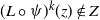 $(L \circ \psi)^k(z) \notin Z$
.
It only remains to prove that (19) holds for all
 $k \geq 0$
. For this purpose fix
 $z \in X$
and note that (19) holds for
 $k = 0$
. We now proceed by induction, assuming that (19) holds for some k and showing that it then holds for
 $k + 1$
as well. First, note that
 \begin{equation*} (L \circ \psi)^{k + 1}(z) = \gamma L(\psi_1((L \circ \psi)^k(z))) + (1 - \gamma) L(\psi_2((L \circ \psi)^k(z))). \end{equation*}
We may compute the first term on the right-hand side by noting that
 \begin{equation*} L\circ\psi_1(x) = \sum_{a \in A} x D_\pi(a)P(a) = x P_\pi \quad \text{for all} \ x \in X. \end{equation*}
Since (19) holds for k, the previous equation implies that
 \begin{align*} \gamma L(\psi_1((L \circ \psi)^k(z))) & = \gamma L(\psi_1(\gamma^k z P_\pi^k + (1 - \gamma) w_k(z))) \\ & = \gamma^{k + 1} z P_\pi^{k + 1} + \gamma (1 - \gamma)w_k(z) P_\pi. \end{align*}
It follows that (19) holds for
 $k + 1$
with
 \begin{equation*} w_{k + 1}(z) \,:\!=\, \gamma (1 - \gamma)w_k(z) P_\pi + (1 - \gamma) L(\psi_2((L \circ \psi)^k(z))). \end{equation*}
The first term on the right-hand side is in
 $\mathbb{R}_+^S$
since
 $w_k(z) \in \mathbb{R}_+^S$
and
 $P_\pi$
has nonnegative entries. Also, the second term is in
 $\mathbb{R}_+^S$
as well since
 $L \circ \psi$
and
 $L \circ \psi_2$
map X into X.
Suppose that the fluid control
 $\phi$
is defined as in (15) in terms of some fluid control
 $\psi$
that satisfies Condition 2. The functions
 $\psi_1$
and
 $\psi_2$
defining
 $\psi$
play different roles in ensuring that the assumptions of Corollary 1 hold. Informally speaking,
 $\psi_1$
is responsible for preventing
 $\beta({\boldsymbol{{x}}}(t))$
from getting stuck at a value strictly smaller than one when
 ${\boldsymbol{{x}}}$
is a fluid trajectory, which is necessary for (13). On the other hand,
 $\psi_2$
ensures that
 $\psi$
complies with the constraints of the problem and thus is indeed a fluid control.
The function
 $\psi_1$
is completely determined by the constants
 $\pi$
, which correspond to a stationary policy for a single process without constraints. Such a policy can be found by inspecting the transition diagrams of a single process for the different actions. Moreover, as noted in Remark 2, there exists
 $\pi$
that satisfies Condition 2 if and only if the policy
 $\nu$
that selects actions uniformly at random satisfies the condition. In contrast, the choice of
 $\psi_2$
depends on the constraints of the problem. In the following two sections we provide rules for defining
 $\psi_2$
when the constraints have specific structures. Nonetheless, we remark that asymptotically optimal policies can be obtained for problems with different constraint structures if an expression for
 $\psi_2$
, such that
 $\psi$
satisfies the constraints, is available.
4.2. Inequality constraints
In this section we impose the following assumption on the constraints.
Assumption 2. The equality constraints are trivial, i.e. we have
 $C(a) = 0$
for all
 $a \in A$
and
 $d = 0$
. In addition, the matrices E(a) are nonnegative, the vector f has strictly positive entries, and there exists
 $0 \in A$
such that
 $E(0) = 0$
.
As noted in Section 2, constraints with nonnegative coefficients as in Assumption 2 can be interpreted as resource allocation constraints. Besides nonnegative coefficients, the assumption imposes two further conditions. The first condition is that there are no equality constraints, which means that it is not compulsory to fully consume any of the resources. The second condition is that there exists an action
 $0 \in A$
that does not consume any of the resources, and can often be interpreted as doing nothing. In this setup, a fluid control that satisfies the assumptions of Corollary 1 exists if the unconstrained single-process problem admits a unichain and aperiodic policy such that the unique irreducible class is contained in
 $S_+^*$
. The following proposition proves this; the proof is provided in Appendix A.
Proposition 3. Suppose that Assumption 2 holds and there exists a set of values
 $\pi$
as in Definition 5 such that the associated matrix
 $P_\pi$
satisfies Condition 2. Define
 \begin{equation*} \gamma \,:\!=\, \min\bigg\{1, \frac{f(k)}{E(i, k, a)} \colon E(i, k, a) \neq 0\bigg\} \in (0, 1] \end{equation*}
and
 $\psi_2 \colon X \longrightarrow Y$
such that
 $\psi_2(x, 0) \,:\!=\, x$
and
 $\psi_2(x, a) \,:\!=\, 0$
for
 $a \neq 0$
. Then Condition 2 holds for the mapping
 $\psi$
defined by
 $\psi(x, a) \,:\!=\, \gamma x D_\pi(a) + (1 - \gamma)\psi_2(x, a)$
for all
 $x \in X$
and
 $a \in A$
.
The proposition gives an expression for a fluid control that satisfies Condition 2. If the constraints (2) do not depend on n, then the following remark provides a simple rounding procedure for defining asymptotically optimal discrete controls.
Remark 3. Suppose that the assumptions of Proposition 3 hold, and
 $E_n(a) = E(a)$
for all
 $a \in A$
and
 $f_n = f$
for all
 $n \geq 1$
. Let
 $\phi$
and
 $\psi$
be as in (15) and Proposition 3, respectively, and define
 $\phi_n \colon X_n \longrightarrow Y_n$
by
 \begin{equation*} \phi_n(x) (i, a) \,:\!=\, \frac{\lfloor n\phi(x) (i, a)\rfloor}{n} \quad \text{for all} \ a \neq 0, \qquad \phi_n(x) (i, 0) = x(i) - \sum_{a \neq 0} \phi_n(x) (i, a) \end{equation*}
for all
 $x \in X_n$
and
 $i \in S$
. In addition, note that
 $\max_{x \in X_n}||\phi(x) - \phi_n(x)||_\infty \leq {|A|}/{n}$
. Note that
 $\phi_n(x)$
puts less weight on the actions
 $a \neq 0$
than
 $\phi(x)$
, and thus
 $\phi_n(x)$
satisfies (2) for all
 $x \in X_n$
. Hence, the functions
 $\phi_n$
are discrete controls for
 $\phi$
. It follows from Corollary 1 and Proposition 3 that these discrete controls are asymptotically optimal.
4.3. Multi-armed restless bandits
Next, we consider multi-armed restless bandit problems with an equality constraint, as stated in the following assumption. Note that multi-armed restless bandit problems with an inequality constraint are already covered by the case under Assumption 2.
Assumption 3. The action space is
 $A = \{0, 1\}$
and there is a unique equality constraint:
 $d \in (0, 1)$
,
 $C(i, 0) = 0$
, and
 $C(i, 1) = 1$
for all
 $i \in S$
. In addition, the inequality constraints are trivial, i.e.
 $E(a) = 0$
for all
 $a \in A$
and
 $f = 0$
.
In this case there is a unique resource which must be fully consumed and there are only two actions. As in Section 4.2, there exists an action
 $0 \in A$
that does not consume the resource and can often be interpreted as doing nothing. In contrast, the other action consumes one unit of resource per arm, regardless of the state the arm is in. The following proposition provides a fluid control that satisfies the assumptions of Corollary 1 if the unconstrained single-arm problem has a unichain and aperiodic policy such that the unique irreducible class is contained in
 $S_+^*$
; the proof is provided in Appendix A.
Proposition 4. Suppose that Assumption 3 holds and there exists a set of values
 $\pi$
as in Definition 5 such that the matrix
 $P_\pi$
satisfies Condition 2. Define
 $\psi_2 \colon X \longrightarrow Y$
by
 \begin{equation*} \psi_2(x)(i, 1) \,:\!=\, \frac{d - \sum_{j \in S} x(j) d \pi(1 \mid j)}{(1 - d)\sum_{j \in S} x(j)[1 - d \pi(1 \mid j)]} x(i)[1 - d \pi(1 \mid i)] \end{equation*}
and
 $\psi_2(x)(i, 0) \,:\!=\, x(i) - \psi_2(x)(i, 1)$
for all
 $i \in S$
. Condition 2 holds with
 \begin{equation*} \psi(x, a) \,:\!=\, d x D_\pi(a) + (1 - d) \psi_2(x, a) \quad \text{for all} \ x \in X, \quad a \in A. \end{equation*}
The following remark provides a simple rounding procedure for defining asymptotically optimal discrete controls using the fluid control defined above.
Remark 4. Suppose that the assumptions of Proposition 4 hold, and that
 $d_n = {\lfloor d n\rfloor}/{n}$
for all
 $n \geq 1$
, which is typically assumed for multi-armed restless bandit problems. Let
 $\phi$
and
 $\psi$
be as in (15) and Proposition 4, respectively, and define
 $\phi_n \colon X_n \longrightarrow Y_n$
as follows. First let
 \begin{equation*} \theta_n(x, i) \,:\!=\, \lfloor d n\rfloor - \sum_{i \in S}\lfloor n\phi(x)(i, 1)\rfloor - \sum_{j = 1}^{i - 1}\mathbf{1}_{\{n\phi(x)(i,1)\notin\mathbb{Z}\}} \quad \text{for all} \ x \in X_n, \quad i \in S, \end{equation*}
where we have enumerated the states, i.e.
 $S = \{1, \ldots, |S|\}$
. Then define
 \begin{equation*} \phi_n(x)(i, 1) \,:\!=\, \begin{cases} \phi(x)(i, 1) & \text{if} \ n\phi(x)(i, 1) \in \mathbb{Z}, \\ [\lfloor n\phi(x)(i, 1)\rfloor + 1]/n & \text{if} \ n\phi(x)(i, 1) \notin \mathbb{Z}, \quad \theta_n(x, i) > 0, \\ \lfloor n\phi(x)(i, 1)\rfloor/n & \text{otherwise}, \end{cases} \end{equation*}
and
 $\phi_n(x)(i, 0) \,:\!=\, x(i) - \phi_n(x)(i, 1)$
for all
 $x \in X_n$
and
 $i \in S$
. This can be interpreted algorithmically as follows. In a first stage, we let
 $\phi_n(x)(i, 1) = \lfloor n\phi(x)(i, 1)\rfloor / n$
for all
 $i \in S$
. If
 $n\phi_n(x)(i, 1) \notin \mathbb{Z}$
for some i, then we must select action 1 for more processes in order to exhaust the budget
 $\lfloor dn\rfloor$
. Therefore, in a second stage, we consider the states i in increasing order and increase
 $\phi_n(x)(i, 1)$
for some states until the budget is exhausted. We increase
 $\phi_n(x)(i, 1)$
by
 $1 / n$
if the budget has not been exhausted yet and
 $n\phi(x)(i, 1) \notin \mathbb{Z}$
. The above expression for
 $\phi_n(x)(i, 1)$
is obtained by noting that the remaining budget when state i is considered equals
 $\theta_n(x, i)$
. It is easy to check that
 $\max_{x \in X_n} ||\phi(x) - \phi_n(x)||_\infty \leq {1}/{n}$
, and that
 $\phi_n(x)$
satisfies the unique equality constraint for all
 $x \in X_n$
. Thus, the functions
 $\phi_n$
are discrete controls for
 $\phi$
. We conclude from Corollary 1 and Proposition 4 that these discrete controls are asymptotically optimal.
5. Examples
Sections 4.2 and 4.3 describe procedures for obtaining asymptotically optimal discrete controls in the cases of resource allocation inequality constraints and multi-armed restless bandits, respectively. In both cases the procedure involves the following steps:
-
(i) Compute an optimal solution
$y^*$
of (4) and define
$x^*$
and
$S_+^*$
as in (14). -
(ii) Find some policy
$\pi$
for the unconstrained single-process problem that is unichain, aperiodic, and such that the unique irreducible class contains
$S_+^*$
. -
(iii) Use
$\pi$
to define a fluid control
$\psi$
as in Proposition 3 or 4, depending on the type of problem, and define a fluid control
$\phi$
as in (15); this solves the fluid problem. -
(iv) Compute a discrete control
$\phi_n$
by rounding the fluid control
$\phi$
as in Remark 3 or 4, depending on the type of problem; this solves the approximation problem.


Step (i) can be carried out numerically. Then Remark 2 can be used to check whether a policy
 $\pi$
as in step (ii) exists, and in that case it is possible to take
 $\pi = \nu$
with
 $\nu$
as in Remark 2. Nonetheless, another good candidate policy is given by
 \begin{equation} \mu(a \mid i) = \begin{cases} {y^*(i, a)}/{x^*(i)} & \text{if} \ x^*(i) > 0, \\ {1}/{|A|} & \text{if} \ x^*(i) = 0. \end{cases}\end{equation}
We have observed empirically that this policy can perform better than
 $\nu$
for finite values of n when it satisfies Condition 2. Also, it has the nice property that
 $x^* D_\mu(a) = y^*(a)$
for all
 $a \in A$
. The remaining steps (iii) and (iv) are straightforward to carry out.
In the following two sections we use the above procedure to obtain discrete controls for concrete problem instances. The policy
 $\mu$
satisfies Condition 2 and is selected in step (ii) in all the cases, with the exception of the problem instance considered in Section 5.2.3. There,
 $\mu$
does not satisfy Condition 2, but
 $\nu$
does and is selected in step (ii). First, we consider a problem with multiple actions and resource allocation inequality constraints as in Section 4.2, and such that the single-process problem is multichain. Then we consider multi-armed restless bandit problems, focusing on different problem instances where the policies proposed in [Reference Hong, Xie, Chen and Wang16, Reference Hong, Xie, Chen and Wang18, Reference Verloop23, Reference Whittle25] are not asymptotically optimal. The discrete controls
 $\phi_n$
satisfy the assumptions of Proposition 3 or 4 in all the cases and therefore are provably asymptotically optimal, as confirmed by our numerical experiments.
5.1. Multiple actions and constraints
Consider a fleet of n electric taxis and suppose that each process describes the battery level of a taxi. Namely,
 $S = \{0, \ldots, 7\}$
are the battery levels and
 ${\boldsymbol{{S}}}_n(t, m)$
represents the battery level at time t of taxi m. Also, the actions
 $A = \{0, 1, 2\}$
are: to deploy the taxi at the airport, to deploy the taxi at the city center, and to charge the taxi, respectively.
The battery level of a taxi that is being charged increases at a constant rate, whereas that of a deployed taxi decreases by a random amount. More precisely, the distribution of
 ${\boldsymbol{{S}}}_n(t + 1, m)$
given that
 ${\boldsymbol{{A}}}_n(t, m) = a$
and
 ${\boldsymbol{{S}}}_n(t, m) = i$
is known and given by

The random variable
 $X_a$
represents the power consumed by a taxi during period t, and tends to be larger for taxis that are deployed at the airport. Specifically,
 $X_a$
has a Poisson distribution with a mean that depends on a in the following way:
 \begin{equation*} \mathbb{P}(X_a = k) \,:\!=\, \frac{\lambda_a^k \mathrm{e}^{-\lambda_a}}{k!} \quad \text{for all} \ k \geq 0, \quad \text{with} \ \lambda_a \,:\!=\, \begin{cases} 2 & \text{if} \ a = 0, \\ 1 & \text{if} \ a = 1. \end{cases}\end{equation*}
At most 70% of the taxis can be charged simultaneously since there are limited charging spots, and the taxi company has agreed with city hall to deploy at least 10% of the fleet at the airport. These constraints can be formulated in such a way that Assumption 2 holds, i.e. by requiring that the following inequalities hold for all
 $t \geq 0$
:
 \begin{equation*} \sum_{i \in S} {\boldsymbol{{y}}}_n(t, i, 2) \leq 0.7, \qquad \sum_{i \in S} [{\boldsymbol{{y}}}_n(t, i, 1) + {\boldsymbol{{y}}}_n(t, i, 2)] \leq 0.9.\end{equation*}
Finally, the rewards are given by

The constants
 $b_a$
and
 $c_a$
can be interpreted as revenues and costs, respectively. On the one hand, taxis deployed at the airport do one trip per period and charge a flat fare
 $b_0 \,:\!=\, 3$
, whereas taxis deployed at the city center charge
 $b_1 \,:\!=\, 2.5$
per unit of distance traveled. On the other hand, a cost
 $c_2 \,:\!=\, 2$
is paid for charging a taxi and penalties
 $c_0 \,:\!=\, 3$
and
 $c_1 \,:\!=\, 2$
are incurred if a taxi is deployed and completely depletes its battery. The rewards defined in this way are plotted in the left panel of Figure 1.
The left panel shows the reward obtained per process and per time step as a function of the state of the process and the action selected. The right panel charts the optimal value of the fluid relaxation, and the gain of the discrete control
 $\phi_n$
when all the batteries are initially empty.

Because the constraints of the problem do not depend on the number of taxis n, it follows from Proposition 1 that the optimal value
 $g_r = 0.8911$
of the fluid relaxation is an upper bound for the gain of any policy. The optimal solution
 $y^*$
of the fluid relaxation that we used to construct a discrete control
 $\phi_n$
is as follows:
 \begin{equation*} y^* = \left[\begin{array}{c@{\quad}c@{\quad}c@{\quad}c@{\quad}c@{\quad}c@{\quad}c@{\quad}c} 0 & 0 & 0 & 0 & 0 & 0 & 0 & 0.1000 \\[4pt] 0 & 0 & 0 & 0 & 0 & 0 & 0.3236 & 0.2095 \\[4pt] 0.0009 & 0.0023 & 0.0100 & 0.0343 & 0.1004 & 0.2189 & 0 & 0 \end{array}\right]\!.\end{equation*}
The constraint that 10% of the fleet is deployed at the airport is satisfied with equality, whereas the other constraint is satisfied with a strict inequality; approximately 37% of the taxis are being charged while 53% of the taxis are in the city center.
The unconstrained single-process problem is multichain, e.g. the policy that always charges the taxi if the battery level is at least 4 and never charges the taxi if the battery level is strictly less than 4 is multichain with absorbing states 0 and 7. However, it is straightforward to check that the policy defined by (20) satisfies Condition 2. It follows that asymptotically optimal discrete controls
 $\phi_n$
can be obtained as explained in Remark 3. The right panel of Figure 1 compares the gains of these discrete controls against the upper bound
 $g_r$
for different values of n; the gains were computed by simulating the processes and averaging the rewards. The plot confirms that the gain of our discrete controls approaches the upper bound.
5.2. Multi-armed restless bandits
We are not aware of any policies for maximizing the expected average reward of weakly coupled processes with more than one constraint. Hence, we compare our assumptions on the transition kernels of the processes with those in the literature for multi-armed restless bandits, which are a narrower class of problems with only two actions and a single constraint with a specific structure. In particular, we consider multi-armed restless bandit problems where the budget constraint is an equality constraint, and we compare our discrete controls with the following four policies: the Whittle index policy proposed in [Reference Whittle25], the LP-priority policies introduced in [Reference Verloop23], the Follow-The-Virtual-Advice (FTVA) policy defined in [Reference Hong, Xie, Chen and Wang16], and the ID policy proposed in [Reference Hong, Xie, Chen and Wang18]. The asymptotic optimality of these policies has been proved in [Reference Gast, Gaujal and Yan9, Reference Gast, Gaujal and Yan10, Reference Hong, Xie, Chen and Wang16, Reference Hong, Xie, Chen and Wang18, Reference Verloop23, Reference Weber and Weiss24] under the assumptions that we discuss below.
-
(i) For the Whittle index and LP-priority policies, the Markov decision process formed by n arms must be unichain for all n as required in [Reference Gast, Gaujal and Yan9, Reference Gast, Gaujal and Yan10, Reference Verloop23, Reference Weber and Weiss24]; in fact, some of these papers even assume that each arm is ergodic.
-
(ii) For the Whittle index policy, the unconstrained single arm must satisfy a condition known as indexability, without which the policy is not well-defined; see [Reference Whittle25].
-
(iii) For the Whittle index and LP-priority policies, a discrete-time dynamical system must satisfy a global attractor property similar to (13); see [Reference Gast, Gaujal and Yan9, Reference Gast, Gaujal and Yan10, Reference Verloop23, Reference Weber and Weiss24]. We do not assume that (13) holds, but prove (13) under the assumption of Proposition 4.
-
(iv) For the FTVA policy, the synchronization assumption defined in [Reference Hong, Xie, Chen and Wang16] must hold.
-
(v) For the ID policy, the single-arm policy (20) must be unichain and aperiodic.
The synchronization assumption pertains to a single-arm problem with a relaxed budget constraint, which must hold on average and not at each time step. Loosely speaking, a system formed by a leader and a follower arm is considered, where the follower arm always selects the same action as the leader arm. The assumption is that there exists an optimal policy, for the aforementioned relaxed single-arm problem, that is unichain and such that the mean time until the leader and follower arms are in the same state is finite. We note that an optimal policy for the above-described relaxed single-arm problem can be obtained as in (20) by standard results for constrained Markov decision processes; see [Reference Altman2].
Conditions (i)–(iii) are significantly stronger than the assumption of Proposition 4, which only requires that the unconstrained single-arm problem admits a unichain and aperiodic policy such that the unique irreducible class contains
 $S_+^*$
. In addition, condition (v) implies that Proposition 4 holds since
 $x^*$
is the stationary distribution of the policy defined by (20) when this policy is unichain and aperiodic. On the other hand, condition (iv) is not entirely understood. However, the synchronization assumption seems to be connected with the existence of suitable aperiodic policies for a single arm; see [Reference Hong, Xie, Chen and Wang16, Appendix C].
Each of the conditions (i)–(v) is violated in one of the examples presented below, and each of the policies for multi-armed bandit problems mentioned above is not asymptotically optimal in one of the examples. In contrast, the assumption of Proposition 4 holds in all the examples, and thus our discrete controls are provably asymptotically optimal.
5.2.1. Counterexamples to Whittle index and LP-priority policies.
In this section we consider two examples where the number of states is three and the single-arm problem is ergodic. Further, the transition probability matrices have positive entries; these matrices, the rewards, and the constraints are provided in Appendix B.
The first example was first considered in [Reference Gast, Gaujal and Khun7] and is nonindexable. In particular, the Whittle index policy is not well-defined. The left panel of Figure 2 compares the gain of different policies with the optimal value
 $g_r = 0.3437$
of the fluid relaxation, which is an upper bound for the gain of any policy. For this particular problem instance, the LP-priority policy outperforms our policy
 $\phi_n$
and the FTVA and ID policies; the latter three policies perform similarly. However, all four policies perform extremely well, with optimality gaps that are less than 3% for
 $n = 200$
and 1% for
 $n = 2000$
.
The left and right panels respectively correspond to the nonindexable problem and the problem where the global attractivity property does not hold for the Whittle index and LP-priority policies.
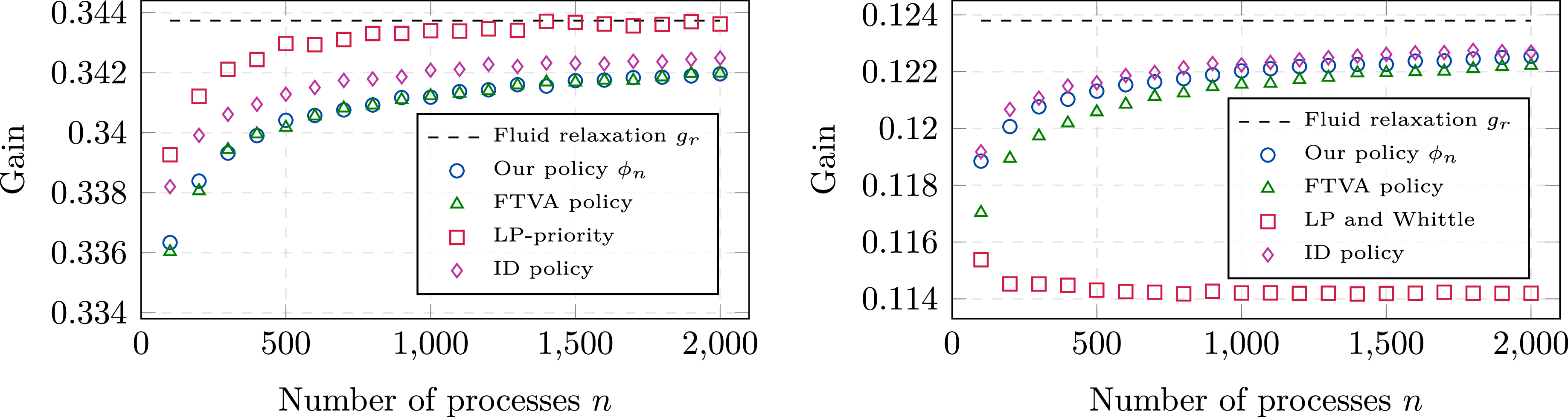
The second example was first considered in [Reference Gast, Gaujal and Yan8] and is such that the global attractivity assumption does not hold for the Whittle index and LP-priority policies, which in this case are the same policy. The plot in the right panel of Figure 2 shows that these policies are not asymptotically optimal for this problem instance. In contrast, our discrete control and the FTVA and ID policies approach
 $g_r = 0.1238$
at similar rates as n grows.
5.2.2. Counterexamples to FTVA.
We now consider an example where the synchronization assumption does not hold and the single-arm problem is multichain. Specifically, the budget constraint is
 $d = 0.25$
, the transition probabilities are depicted in Figure 3, and the rewards are given by
 \begin{equation*} r = \left[\begin{array}{l@{\quad}l@{\quad}l@{\quad}l@{\quad}l} 0 & 0 & 1 & 0 & 1 \\ 0 & 0 & 0 & 1 & 0 \end{array}\right]\!.\end{equation*}
The diagrams depict the transition probabilities for both actions. The plot compares the optimal value of the fluid relaxation and the gain of several policies. The gains were computed by simulating systems where all the arms are initially in state 0.

In order to show that the synchronization assumption does not hold, let us consider the single-arm problem with the relaxed budget constraint, i.e. action 1 must be selected 25% of the time. Consider also the following policy for this problem:
 $\pi(0 \mid i) = 1$
if
 $i \in \{2, 4\}$
and
 $\pi(1 \mid i) = 1$
if
 $i \in \{0, 1, 3\}$
. This policy is unichain and aperiodic, and the probability that action 1 is selected in steady state is
 $0.25$
. Hence,
 $\pi$
is a feasible solution, and it is easy to check that its gain is 1, which is clearly the maximum gain that any policy can achieve. It is also possible to check that any other policy with gain 1 must coincide with
 $\pi$
in states 2, 3, and 4. Moreover, the set
 $\{2, 3, 4\}$
must be absorbing for the Markov chain associated with the policy.
Suppose now that a leader arm uses one of the optimal policies while a follower arm always selects the same action as the leader arm. Assume also that the leader and follower arms are in states 2 and 0 at time zero, respectively. Since the leader arm remains within
 $\{2, 3, 4\}$
, it can never select action 1 twice in a row and therefore the follower arm can never leave
 $\{0, 1\}$
. It follows that the synchronization assumption does not hold, and the plot in Figure 3 shows that FTVA is not asymptotically optimal if all the arms are initially in state 0. Similar counterexamples to FTVA are constructed in [Reference Hong, Xie, Chen and Wang18]; these examples satisfy the assumptions in [Reference Hong, Xie, Chen and Wang18] and thus also our weaker assumptions.
States 2 and 3 have the lowest and highest Whittle indexes, respectively, and our numeric computations indicate that the other three states have a common Whittle index that is strictly between the indexes of 2 and 3. If we arrange the states as (3, 1, 0, 4, 2), then we obtain the Whittle index policy plotted in Figure 3, which is also an LP-priority policy; arranging the states as (3, 1, 0, 2, 4), we obtain another LP-priority policy with nearly the same performance. However, there are no results that rigorously establish this asymptotic optimality because the example considered here is multichain and all the available results concern unichain setups. In contrast, our discrete controls
 $\phi_n$
and the ID policy are provably asymptotically optimal for this problem instance, as confirmed by Figure 3.
5.2.3. Counterexample to ID policy.
Finally, we consider multi-armed restless bandits with budget constraint
 $d = 0.5$
and the transition probabilities and rewards depicted in Figure 4. The objective of the fluid relaxation (4) is to maximize
 $y(0, 0) + y(1, 1) \leq 1$
, and
 $\max\{y(0, 0), y(1, 1)\} \leq 0.5$
by the budget constraint since at most half of the processes can use action 0 and at most half of the processes can use action 1. Then it is not difficult to check that there exists a unique solution
 $y^*$
which is given by
 $y^*(0, 0) = y^*(1, 1) = 0.5$
and
 $y^*(i, a) = 0$
otherwise.
The diagrams depict the transition probabilities and rewards for both actions; all the transitions are deterministic. The chart compares the optimal value of the fluid relaxation and the gain of different policies; the gains were computed by simulating systems where all the arms are initially in state 0.

Consider now the single-arm policy
 $\mu$
defined by (20) when
 $y^*$
is as above. State 2 is transient while states 0 and 1 form an irreducible class with period 2. The synchronization assumption used in [Reference Hong, Xie, Chen and Wang16] does not hold because a leader starting in state 0 and a follower starting in state 2 will never be in the same state. In addition, the assumptions used in [Reference Hong, Xie, Chen and Wang18] to establish the asymptotic optimality of the ID policy do not hold either since
 $\mu$
is not aperiodic. However, the policy
 $\nu$
that selects actions uniformly at random is ergodic and thus yields discrete controls
 $\phi_n$
that are asymptotically optimal by Proposition 4.
The plot in Figure 4 confirms that our discrete controls
 $\phi_n$
are asymptotically optimal and further shows that all the other policies have gains that are far from the optimal value when all the arms are in state 0 at time zero. In fact, it is not difficult to check analytically that the Whittle index, LP-priority, and ID policies have gains equal to
 $\frac12$
.
For example, consider the ID policy, which follows the policy
 $\mu$
defined by (20) for as many arms as possible. More specifically, a permanent and unique ID in
 $\{1, \ldots, n\}$
is assigned to each arm at time
 $t = 0$
. Then, at each time, an action is sampled for each arm using the single-arm policy
 $\mu$
, and the sampled action is applied to the arms in order of their IDs for as many arms as allowed by the budget constraint; the actions for the rest of the arms are chosen so as to comply with the constraint. For the problem described in Figure 4, the action sampled at time
 $t = 0$
is 0 for all the arms. Hence, the half of the arms having the lowest IDs will move to state 1 at
 $t = 1$
, while the rest of the arms will move to state 2. Then the action sampled for the arms in state 1 will be 1 because
 $\mu$
is deterministic at state 1. Since these arms have the lowest IDs, action 1 will be used for these arms and action 0 will be used for the other arms. It follows that the state of the entire system at
 $t = 2$
is exactly the same as at
 $t = 0$
and that the system evolves periodically in the way just described. We conclude that half of the arms will obtain a reward equal to 1 at each time step while the other half will not obtain any reward.
Noting that the Whittle index and LP-priority policy give the highest priority for using action 1 in state 1, similar arguments as above can be used to show that both policies have gain
 $\frac12$
. The gain of the FTVA policy may depend on the tie-breaking rule used to decide which arms follow the virtual advice; the tie-breaking rule used in our simulations is the same as we described above for the ID policy. Nonetheless, we recall that the synchronization assumption does not hold for this problem instance.
6. Concluding remarks
We have established that asymptotically optimal policies for weakly coupled Markov decision processes can be obtained essentially by solving a fluid counterpart of the problem and then constructing discrete approximations of the solution. We have further derived sufficient conditions for the existence of a fluid control that solves the fluid problem and structural properties that help to construct such a fluid control. Moreover, we have used these conditions and structural properties to construct asymptotically optimal policies for multi-armed restless bandits and a broad class of problems with multiple actions and inequality constraints. In these setups, we showed that a sufficient condition for asymptotic optimality is that the unconstrained single-process problem admits a suitable unichain and aperiodic policy, and we provided multichain examples where this condition holds.
While most of our results hold for problems with general constraints, the asymptotically optimal policies are constructed explicitly only for multi-armed restless bandits and the above-mentioned class of problems with multiple actions and inequality constraints. An interesting topic for future research is the explicit construction of asymptotically optimal policies for problems with a different structure. In addition, the present paper focuses on obtaining asymptotically optimal policies under very general assumptions, but it would be interesting to study how the optimality gap of our policies depends on the number of processes, possibly under more restrictive assumptions. Our numerical experiments suggest that this dependence may vary across different problem instances.
Appendix A. Proofs of various results
Proof of Proposition
1. Fix n satisfying (5) and let
 $\pi \in \Pi_n^{SR}$
and
 $s \in S^n$
. By [Reference Puterman21, Proposition 8.1.1],
 \begin{equation} y_n(i, a) \,:\!=\, \lim_{T\to\infty}\frac{1}{T}\sum_{t = 0}^{T - 1}\mathbb{E}_s^\pi[{\boldsymbol{{y}}}_n(t, i, a)] \end{equation}
exists for all
 $i \in S$
and
 $a \in A$
; the limit clearly depends on the specific policy
 $\pi$
and initial state s, but we omit them from the notation for brevity. We claim that
 \begin{align} &\sum_{a \in A} y_n(a)P(a) = \sum_{a \in A} y_n(a), \\[-12pt] \nonumber \end{align}
 \begin{align} &\sum_{a \in A} y_n(a)C_n(a) = d_n, \\[-12pt] \nonumber \end{align}
 \begin{align} &\sum_{a \in A} y_n(a)E_n(a) \preceq f_n, \\[-12pt] \nonumber \end{align}
 \begin{align} &y_n \in Y. \\[6pt] \nonumber \end{align}
Suppose that (22) holds for all the stationary policies
 $\pi$
and initial states s. If (5) also holds, then
 $y_n$
is a feasible solution of the fluid relaxation, and thus
 $g_n^\pi(s) = \sum_{a \in A} y_n(a) r(a) \leq g_r$
. Since the stationary policy
 $\pi$
and initial state s are arbitrary, this proves the first claim of the proposition.
For the second claim, we argue by contradiction. If (6) does not hold, then there exist stationary policies and initial states
 $\{\pi_k, s_k \colon k \in \mathcal{K}\}$
such that
 $\lim_{k \to \infty} g_k^{\pi_k}(s_k) > g_r$
, where
 $\mathcal{K} \subset \mathbb{N}$
is infinite. Define
 $y_k$
in terms of
 $\pi_k$
and
 $s_k$
as in (21). It follows from (22) and the compactness of Y that the sequence
 $\{y_k \colon k \in \mathcal{K}\}$
has a limit point y that is a feasible solution of (4). By taking a subsequence, we may assume without any loss of generality that
 $y_k \to y$
as
 $k \to \infty$
, which leads to the following contradiction:
 \begin{equation*} \lim_{k \to \infty} g_k^{\pi_k}(s_k) = \lim_{k \to \infty} \sum_{a \in A} y_k(a)r(a) = \sum_{a \in A} y(a)r(a) \leq g_r. \end{equation*}
It only remains to prove that (22) holds for all
 $\pi \in \Pi_n^\mathrm{SR}$
and
 $s \in S^n$
. We only prove (22a) since the other properties follow from similar arguments. For this purpose, note that
 \begin{equation*} \sum_{a \in A} \mathbb{E}_s^\pi[{\boldsymbol{{y}}}_n(t, a)] P(a) = \sum_{a \in A} \mathbb{E}_s^\pi[{\boldsymbol{{y}}}_n(t + 1, a)] \quad \text{for all} \ t \geq 0 \end{equation*}
by (1). Taking the Cesàro limit as
 $t \to \infty$
on both sides of the equation, we conclude that the vector
 $y_n$
defined by (21) indeed satisfies (22a).
Proof of Lemma
1. Consider the random variables
 $U_t^l(j \mid i, a) \,:\!=\, B_t^l(j \mid i , a) - p(j \mid i, a)$
and
 $V_t^l(i, a) \,:\!=\, \mathbf{1}_{\{n{\boldsymbol{{y}}}_n(t - 1, i, a) \geq l\}}$
. Now let us fix
 $t \geq 1$
and
 $j \in S$
, and note that we may write
 \begin{equation*} {\boldsymbol{{z}}}_n(t, j) = \frac{1}{n} \sum_{l = 1}^n \sum_{i \in S} \sum_{a \in A} W_t^l(j \mid i, a) \quad \text{with} \ W_t^l(j \mid i, a) \,:\!=\, U_t^l(j \mid i, a)V_t^l(i, a). \end{equation*}
If
 $l_1 \neq l_2$
,
 $i_1 \neq i_2$
, or
 $a_1 \neq a_2$
, then
 \begin{equation*} \mathbb{E}[{W_t^{l_1}(j \mid i_1, a_1)W_t^{l_2}(j \mid i_2, a_2)}] = \mathbb{E}[U_t^{l_1}(j \mid i_1, a_1)]\mathbb{E}[V_t^{l_1}(i_1, a_1)W_t^{l_2}(j \mid i_2, a_2)] = 0 \end{equation*}
because
 $U_t^{l_1}(j \mid i_1, a_1)$
is independent of
 ${\boldsymbol{{y}}}_n(t - 1)$
and
 $U_t^{l_2}(j \mid i_2, a_2)$
. Furthermore,
 \begin{align*} \mathbb{E}[(W_t^l(j \mid i, a))^2] & = \mathbb{E}[(U_t^l(j \mid i, a))^2] \mathbb{E}[(V_t^l(i, a))^2] \\ & = [1 - p(j \mid i, a)]p(j \mid i, a)\mathbb{P}(n{\boldsymbol{{y}}}_n(t - 1, i, a) \geq l) \end{align*}
for all
 $l \geq 1$
,
 $i \in S$
, and
 $a \in A$
. We conclude that
 \begin{align*} \mathbb{E}[{\boldsymbol{{z}}}_n^2(t, j)] & = \frac{1}{n^2}\sum_{l = 1}^n \sum_{i \in S} \sum_{a \in A} [1 - p(j \mid i, a)]p(j \mid i, a)\mathbb{P}(n{\boldsymbol{{y}}}_n(t - 1, i, a) \geq l) \\ & \leq \frac{1}{n^2} \sum_{i \in S} \sum_{a \in A} q_{\max}(j)p(j \mid i, a) \mathbb{E}[n{\boldsymbol{{y}}}_n(t - 1, i, a)] = \frac{q_{\max}(j)}{n}\mathbb{E}[{\boldsymbol{{x}}}_n(t, j)]. \end{align*}
The other inequality is obtained using similar arguments.
Proof of Lemma
3. Suppose that
 $x \in X$
and
 $x \neq x^*$
. Then
 $\beta(x) = \beta(x) x^* e \leq x e = 1$
, where e is the column vector of ones. It is clear that
 $\beta(x) \neq 1$
since otherwise
 $x = x^*$
, so we conclude that
 $1 - \beta(x) > 0$
, and thus (i) follows from
 $[1 - \beta(x)]^{-1}[x - \beta(x)x^*] e = 1$
.
Recall that
 $S_+^* \,:\!=\, \{i \in S \colon x^*(i) > 0\}$
. For each
 $\lambda \geq 0$
, we have
 \begin{align*} \beta^{-1}((\lambda, \infty)) & = \{x \in \mathbb{R}_+^S \colon x(i) > \lambda x^*(i)\ \text{for all}\ i \in S^*\}, \\ \beta^{-1}([\lambda, \infty)) & = \{x \in \mathbb{R}_+^S \colon x(i) \geq \lambda x^*(i)\ \text{for all}\ i \in S^*\}. \end{align*}
These sets are open and closed in
 $\mathbb{R}_+^S$
, respectively. Therefore,
 \begin{equation*} \beta^{-1}((\lambda, \mu)) = \beta^{-1}((\lambda, \infty)) \setminus \beta^{-1}([\mu, \infty)), \qquad \beta^{-1}([0, \mu)) = \mathbb{R}_+^S \setminus \beta^{-1}([\mu, \infty)) \end{equation*}
are open in
 $\mathbb{R}_+^S$
for all
 $\lambda \geq 0$
and
 $\mu > 0$
, which proves (ii).
Proof of Proposition
3. We only need to check that
 $\psi$
is a fluid control. First, note that
 \begin{equation*} \sum_{a \in A} \psi(x, a) = \gamma x \sum_{a \in A} D_\pi(a) + (1 - \gamma) x = x \quad \text{for all} \ x \in X. \end{equation*}
Furthermore, the inequality constraints hold since
 \begin{equation*} \sum_{a \neq 0}\sum_{i \in S} \gamma x(i)\pi(a \mid i)E(i, k, a) \leq \gamma \max \{E(i, k, a) \colon i \in S, a \neq 0\} \leq f(k) \quad \text{for all} \ x \in X \end{equation*}
and all k less than or equal to the dimension of f. Hence, Definition 2 holds.
Proof of Proposition
4. Since
 $d < 1$
,
 $\varepsilon \,:\!=\, \min_{i \in S} [1 - d \pi(1 \mid i)] > 0$
. Hence, the denominator in the definition of
 $\psi_2(x)(i, 1)$
is lower bounded by
 $(1 - d)\varepsilon$
. This implies that
 $\psi_2$
is well-defined, and clearly also continuous.
It only remains to check that
 $\psi$
is a fluid control. First, note that
 \begin{equation*} \sum_{a \in A} \psi(x, a) = d x \sum_{a \in A} D_\pi(a) + (1 - d) \sum_{a \in A} \psi_2(x, a) = d x + (1 - d)x = x \end{equation*}
because
 $\psi_2(x, 0) + \psi_2(x, 1) = x$
by definition. Moreover,
 \begin{align*} \sum_{i \in S} \psi(x)(i, 1) & = \sum_{i \in S} x(i) d \pi(1 \mid i) + \sum_{i \in S} (1 - d)\psi_2(x)(i, 1) \\ & = \sum_{i \in S} x(i) d \pi(1 \mid i) + \sum_{i \in S} \frac{d - \sum_{j \in S} x(j) d \pi(1 \mid j)}{\sum_{j \in S} x(j)[1 - d \pi(1 \mid j)]} x(i)[1 - d \pi(1 \mid i)] = d, \end{align*}
which means that
 $\psi$
complies with the unique equality constraint.
Appendix B. Details of the examples
The transition probability matrices for the nonindexable example of Section 5.2.1 are:
 \begin{equation*} P(0) = \left[\begin{array}{l@{\quad}l@{\quad}l} 0.0050 & 0.7930 & 0.2020 \\ 0.0270 & 0.5580 & 0.4150 \\ 0.7360 & 0.2490 & 0.0150 \end{array}\right]\!, \qquad P(1) = \left[\begin{array}{l@{\quad}l@{\quad}l} 0.7180 & 0.2540 & 0.0280 \\ 0.3470 & 0.0970 & 0.5560 \\ 0.0150 & 0.9560 & 0.0290 \end{array}\right]\!.\end{equation*}
In addition, the budget constraint is
 $d = 0.5$
and the rewards are given by
 \begin{equation*} r = \left[\begin{array}{c@{\quad}c@{\quad}c} 0 & 0 & 0 \\ 0.6990 & 0.3620 & 0.7150 \end{array}\right]\!.\end{equation*}
The transition probability matrices for the other example of Section 5.2.1 are:
 \begin{equation*} P(0) = \left[\begin{array}{l@{\quad}l@{\quad}l} 0.0223 & 0.1023 & 0.8754 \\ 0.0343 & 0.1718 & 0.7940 \\ 0.5232 & 0.4552 & 0.0215 \end{array}\right]\!, \qquad P(1) = \left[\begin{array}{l@{\quad}l@{\quad}l} 0.1487 & 0.3044 & 0.5469 \\ 0.5685 & 0.4112 & 0.0204 \\ 0.2527 & 0.2731 & 0.4742 \end{array}\right]\!.\end{equation*}
Also, the budget constraint is
 $d = 0.4$
and the rewards are given by
 \begin{equation*} r = \left[\begin{array}{c@{\quad}c@{\quad}c} 0 & 0 & 0 \\ 0.3740 & 0.1174 & 0.0787 \end{array}\right]\!.\end{equation*}
Funding information
Most of this work was carried out while Diego Goldsztajn was with Inria, funded by an Inria fellowship. Part of this work was supported by ANII Uruguay through the fellowship PD_NAC_2024_1_182118.
Competing interests
There were no competing interests to declare which arose during the preparation or publication process of this article.
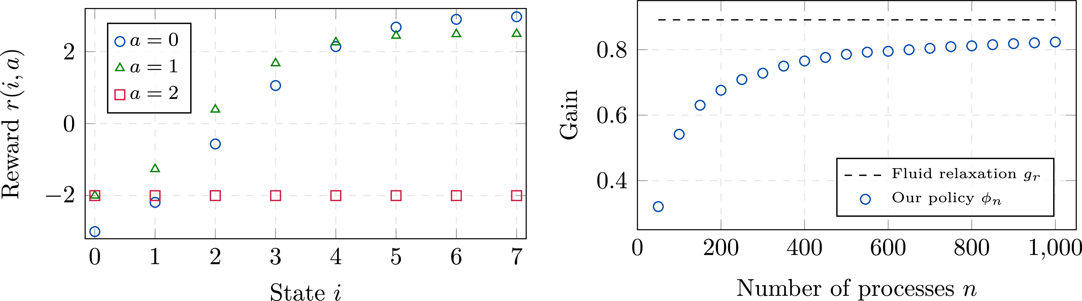
 ϕn