





Impact Statement
Underwater infrastructure inspection generates thousands of images with inconsistent quality, requiring manual curation before processing, which is a costly bottleneck for inspection agencies evaluating bridge piers, dams, and offshore structures. This work presents an unsupervised scene-based clustering framework that automatically organizes underwater imagery by environmental conditions without requiring labeled training data or specialized sensors. The approach integrates with existing robotic systems to prefilter degraded images before reconstruction pipelines, directly reducing computational costs and improving photogrammetry accuracy. By demonstrating that scene-based clustering enhances feature matching robustness across varying illumination and viewpoint conditions, this methodology enables inspection practitioners to process large-scale robotic surveys more efficiently. The framework supports rapid condition assessment documentation and postdisaster evaluation workflows, making it immediately applicable to infrastructure monitoring operations.
1. Introduction
The inspection of submerged infrastructure components, such as marine structures and bridge piers, has long been a challenging task. Routine inspections are essential to maintaining resiliency, and emergency assessments must be done rapidly after a disaster event. Traditionally, such inspections are performed visually by highly trained dive inspectors. These inspections are time-intensive and disruptive, and the limited number of sufficiently trained divers can be problematic in emergency situations. Modern robotic systems combined with digital imaging and computer vision analysis offer an opportunity to improve the inspection process. However, the underwater environment poses unique challenges for computer vision algorithms, particularly for robotic imaging, where the resulting image set is typically unstructured and often decontextualized.
Scene understanding is a central task for many computer vision applications. Given an understanding of a scene with respect to lighting, color, image quality, and content, many downstream tasks such as photogrammetric reconstruction or real-time assessments can be enhanced and expedited. In the context of the inspection of submerged infrastructure, applications include data set optimization for 3D reconstruction of infrastructure components and support for mandated element (component) level inspection processes.
The value of organizing images prior to structure from motion (SfM) reconstruction has been established in large-scale terrestrial photogrammetry, as demonstrated on internet-scale SfM pipelines (Frahm et al., Reference Frahm, Fite-Georgel, Gallup, Johnson, Raguram, Wu, Jen, Dunn, Clipp, Lazebnik, Pollefeys, Daniilidis, Maragos and Paragios2010). More recently, a cluster-based system was developed (Li et al., Reference Li, Qi, Wang and Bao2023) where camera graphs are divided into subgraphs via clustering algorithms in the sparse point-cloud reconstruction stage, with multiple computational nodes executing local SfM on clustered subsets to improve efficiency and feature matching accuracy. In aerial photogrammetry, a hierarchical clustering (HC)-aligning framework (Xie et al., Reference Xie, Yang, Li, Li and Zhang2019) demonstrated significant efficiency improvements in reconstruction. Hierarchical image organization strategies, such as triplet-based linking (Michelini and Mayer, Reference Michelini and Mayer2020), have further demonstrated robustness for complex datasets with varying camera baselines.
Underwater environments introduce additional challenges that make scene-based preprocessing not merely advantageous but essential. For underwater robotic imaging, these advantages are amplified: abrupt scene transitions, depth-dependent attenuation, variable artificial illumination, and frames corrupted by diffraction, bubbles, backscatter, or motion blur can produce false correspondences and degrade global optimization. Scene-level clustering therefore (i) facilitates automated exclusion or separate handling of image subsets that are unsuitable for reconstruction, (ii) increases the inlier ratio during local matching by limiting comparisons to photometrically consistent images, and (iii) enables efficient, parallel local SfM workflows that reduce wall-time and memory pressure prior to global bundle adjustment.
Given that a robotic inspection often includes many thousands of unstructured images, scene understanding is a nontrivial task critical to efficient assessment (Spencer et al., Reference Spencer, Hoskere and Narazaki2019). In this context, clustering facilitates targeted analysis by isolating infrastructure components and supporting downstream computer vision tasks such as 3D reconstruction and image stitching. The underwater environment poses significant challenges for scene understanding due to the intrinsic variability of aquatic settings, influenced by factors such as water depth (Sankpal and Deshpande, Reference Sankpal and Deshpande2016) and illumination (O’Byrne et al., Reference O’Byrne, Schoefs, Pakrashi and Ghosh2018). Light interaction with water leads to scattering and absorption, collectively termed attenuation (Sankpal and Deshpande, Reference Sankpal and Deshpande2016). Additional environmental factors, including particulates (Duarte et al., Reference Duarte, Codevilla, Gaya and Botelho2016; Peng and Cosman, Reference Peng and Cosman2017) and fluctuating underwater illumination (flicker) (Swirski and Schechner, Reference Swirski and Schechner2013), further degrade image quality. Inherent distortions such as reduced chroma, low contrast, blurring, non-uniform color casting, and noise, significantly undermine image quality and alter color consistency and contrast (Peng and Cosman, Reference Peng and Cosman2017; Wang et al., Reference Wang, Song, Fortino, Qi, Zhang and Liotta2019). These complexities necessitate specialized techniques for effective underwater image processing.
Preprocessing strategies for underwater images are influenced by scene characteristics and are closely tied to water’s spectral properties (Monterroso Muñoz et al., Reference Monterroso Muñoz, Moron-Fernández, Cascado-Caballero, Diaz-del-Rio and Real2023). Research in underwater imaging has focused on enhancement and restoration techniques (Li et al., Reference Li, Quo, Pang, Chen and Wang2016; Sankpal and Deshpande, Reference Sankpal and Deshpande2016; Berman et al., Reference Berman, Treibitz and Avidan2017; Wang et al., Reference Wang, Song, Fortino, Qi, Zhang and Liotta2019; Yang et al., Reference Yang, Hu, Li, Rohde, Du and Hu2019), with enhancement often preferred for its simplicity and independence from water parameter estimation. The development of specialized datasets has further facilitated training and evaluation of machine learning models tailored to underwater conditions (O’Byrne et al., Reference O’Byrne, Schoefs, Pakrashi and Ghosh2018, Reference O’Byrne, Ghosh, Schoefs and Pakrashi2020; Yang et al., Reference Yang, Hu, Li, Rohde, Du and Hu2019). However, deep learning remains limited by its reliance on extensive labeled datasets and computationally intensive tuning that are often impractical for highly varied underwater scenes (Yedida et al., Reference Yedida, Yang and Menzies2022; Vijayalakshmi and Sasithradevi, Reference Vijayalakshmi and Sasithradevi2024). This has driven interest in single-image processing methods that utilize intrinsic underwater image properties without exhaustive external calibration (Wang et al., Reference Wang, Song, Fortino, Qi, Zhang and Liotta2019). Expanding on this, scene-based clustering approaches offer a means to address the absence of standardized references for water types and environmental conditions (Sankpal and Deshpande, Reference Sankpal and Deshpande2016), improving underwater image analysis through global feature evaluation. It also provides a means to structure underwater image datasets, improving feature matching and global feature evaluation, thereby mitigating the challenges posed by unstructured robotic imaging.
1.1. Related prior work
Content-based image annotation and retrieval are applications of image clustering, and significant advancements have been made in the field of image clustering across different domains (Chang et al., Reference Chang, Wang, Meng, Xiang and Pan2017; Ren et al., Reference Ren, Wang, Li and Xu2020). However, research has primarily focused on object-centric analysis rather than on the scene-level understanding necessary in the inspection context.
Underwater image clustering commonly incorporates background light (BL) analysis and feature extraction targeting local or global attributes (Ping Tian, Reference Ping Tian2013; Tekli, Reference Tekli2022). Key features include color (Qiu, Reference Qiu2003; Shao et al., Reference Shao, Wu, Cui and Zhang2008; Duanmu, Reference Duanmu2010) and texture assessment (Aziz and Othman, Reference Aziz and Othman2017; Sutojo et al., Reference Sutojo, Tirajani, Ignatius Moses Setiadi, Sari and Rachmawanto2017) that can be combined to enhance interpretability in complex scenes (Taheri et al., Reference Taheri, Rahbar and Salimi2023). However, choosing appropriate metrics remains challenging due to the multifaceted nature of water clarity, typically measured by turbidity, Secchi depth, light attenuation, or other quality-related indices.
Although light attenuation is the most precise measure of water visibility, proxy metrics such as Secchi depth and turbidity are more cost-effective for practical applications (Turner et al., Reference Turner, Fall and Friedrichs2023). The study presented in (Rudy and Wilson, Reference Rudy and Wilson2024) introduces Turbidivision, a machine vision-based application for estimating turbidity from underwater images. The approach consists of a two-step model: an image classification network trained on turbidity-labeled images, followed by a regression model to provide continuous estimates. The dataset used for training includes a combination of in situ field data and controlled lab mesocosms, covering a range of suspended sediment concentrations and colorimetric conditions, with and without a Secchi disk as a visual reference. The model demonstrates high classification accuracy and provides reasonable turbidity estimations suitable for applications where lower precision is acceptable.
Image quality is affected by factors such as the optical performance of the equipment, instrument noise, imaging conditions, and processing techniques (Wang et al., Reference Wang, Song, Fortino, Qi, Zhang and Liotta2019). Recent literature highlights computational metrics tailored for underwater imaging (Shahid et al., Reference Shahid, Rossholm, Lövström and Zepernick2014; Zhai and Min, Reference Zhai and Min2020; Moghimi and Mohanna, Reference Moghimi and Mohanna2021; Hao et al., Reference Hao, Yuan, Zhang and Zhang2024). For instance, the Underwater Color Image Quality Evaluation (UCIQE) metric assesses fuzziness, contrast, and color cast (Yang and Sowmya, Reference Yang and Sowmya2015), while the Underwater Image Quality Measure (UIQM) integrates colorfulness (UICM), sharpness (UISM), and contrast (UIConM) (Panetta et al., Reference Panetta, Gao and Agaian2016).
Advanced turbidity methods, such as URanker, incorporate convolutional-attentional Transformers with histogram priors and dynamic cross-scale correspondence, providing improved quality assessment under local degradation (Guo et al., Reference Guo, Wu, Jin, Han, Chai, Zhang and Li2022). While these metrics approximate turbidity, they do not yield absolute turbidity measurements. Relative approaches aggregating edge strength and saturation (Zheng et al., Reference Zheng, Lu, Wang, Zhang and Guizani2024) provide spatially adaptive turbidity estimates but lack absolute quantification, necessitating condition-specific methodologies. Addressing this limitation, Karnawat and Patil (Reference Karnawat and Patil2016) propose a turbidity estimation method based on high-definition image processing. The approach involves RGB (Red-Green-Blue) to-gray conversion, noise filtration, histogram analysis, and thresholding, with turbidity levels calibrated against a laboratory-based reference dataset.
Critically, datasets such as the simulated water type dataset facilitate benchmarking by simulating diverse aquatic conditions that represent different Jerlov water types (Raihan et al., Reference Raihan, Abas and De Silva2021). This allows the research community to test featurization and characterization algorithms on established and curated test sets.
1.1.1. Applications of underwater scene analysis in civil engineering
Maintaining consistent lighting, radiometric color accuracy, and robust feature matching are critical for photogrammetric documentation of submerged cultural heritage sites, and scene clustering enables adaptive reconstruction strategies tailored to specific scene characteristics (Diamanti and Ødegård, Reference Diamanti and Ødegård2024). A relevant example is offered by Johnson-Roberson et al. (Reference Johnson-Roberson, Bryson, Friedman, Pizarro, Troni, Ozog and Henderson2017), which presents a high-resolution underwater mapping and 3D reconstruction method that achieves a 2 mm/pixel resolution using an AUV alongside a diver-operated stereo imaging platform. To address color constancy issues from frequency-dependent light attenuation, a two-layered clustering approach is used: first segmenting images by altitude bands, then grouping them by seabed type (e.g., rocks, stones, sand). This unsupervised method improves subset homogeneity, enabling precise pixel-level corrections and consistent color normalization across varying underwater conditions.
An application relevant to photogrammetry and structural reconstruction is presented in Yu et al. (Reference Yu, Shen, Zhang and Xiang2024), which focuses on underwater structural integrity assessment by integrating semantic segmentation, geometric quantification, and voxel neural radiance fields. Utilizing a wall-climbing robot equipped with high-definition cameras, this system successfully detects structural cracks and performs 3D reconstructions of an underwater pier in a prestressed concrete bridge. However, the study highlights persistent challenges, including image distortion due to bubbles and lighting-induced shadows that make some frames unusable.
Parallel to underwater inspection, deep learning frameworks for tunnel infrastructure have demonstrated automated defect classification from ground-penetrating radar profiles using convolutional networks and vision transformers with hierarchical classification strategies (Rosso et al., Reference Rosso, Marasco, Aiello, Aloisio, Chiaia and Marano2023, Reference Rosso, Aloisio, Randazzo, Tanzi, Cirrincione and Marano2024).
1.2. Research gaps addressed in this study
Current underwater image analysis methods focus on object-level classification, and there is a lack of studies on scene-based clustering methods that are essential for efficient dataset organization, curation, and underwater structural health monitoring (SHM) more generally. This is particularly true for 3D computer vision methods such as photogrammetry. Environmental variability degrades feature matching reliability, causing inconsistencies in keypoint detection and image alignment. Existing computer vision pipelines do not incorporate scene-aware clustering, leading to suboptimal reconstruction accuracy and higher computational costs. Additionally, no standardized evaluation framework exists for clustering underwater images based on scene attributes, limiting reproducibility and benchmarking of clustering methodologies.
Table 1 contrasts the proposed approach with existing underwater image analysis methods reviewed in Section 1.1. The key distinctions are highlighted across six dimensions, clarifying how scene-based unsupervised clustering addresses limitations of supervised approaches and quality metrics that lack clustering capabilities.
Comparison of the proposed framework with existing underwater image analysis methods

Table 1. Long description
The table consists of seven columns: Method, Analysis level, Supervision, Multi-feature integration, Clustering output, Validation approach, and S H M application.
* Turbidivision (Rudy and Wilson, 2024): Focuses on turbidity estimation using supervised labeled data. It uses a single metric, outputs turbidity classes, validates via prediction accuracy, and has limited S H M application.
* URanker (Guo et al., 2022): Focuses on image quality ranking using supervised learned priors. It integrates histogram and spatial features, provides ranking without clustering, validates via quality score correlation, and has no S H M application.
* U C I Q E / U I Q M (Yang and Sowmya, 2015; Panetta et al., 2016): Focuses on image quality assessment using unsupervised methods. It uses partial predefined metrics, has no clustering, validates via human perception correlation, and has indirect S H M application.
* Altitude-based (Johnson-Roberson et al., 2017): Focuses on scene segmentation using unsupervised depth-based data. It does not integrate multiple features, provides spatial clustering, validates via 3D reconstruction quality, and requires depth sensors for S H M application.
* Scene-based clustering (proposed): Focuses on scene characterization using unsupervised methods. It integrates color, texture, clarity, and quality features. It provides scene-based clusters, validates via feature matching and 3D alignment, and is suitable for vision-only S H M applications.
1.3. Contributions of this study
This study introduces a scene-based clustering framework for underwater SHM, shifting from object-level analysis to global scene understanding without relying on curated reference images. The proposed approach integrates multiscale feature extraction, correlation analysis, and dimensionality reduction to enhance robustness against variability, optimizing feature selection for turbidity assessment and underwater scene characterization.
Validated using hierarchical and centroid-based clustering algorithms, the framework effectively organizes unlabeled datasets and evaluates class-to-cluster mapping in labeled scene-based underwater datasets. Applied to real-world SHM scenarios and controlled laboratory experiments, it improves keypoint detection, feature correspondence, and image alignment accuracy, reducing mismatches caused by lighting variations and turbidity. A comprehensive performance evaluation using clustering validity metrics also demonstrates its effectiveness. Additionally, by optimizing dataset structuring for SfM and image stitching, the framework enhances computational efficiency in feature-based reconstruction pipelines. This study establishes scene-aware clustering as a scalable, interpretable approach for improving dataset organization and feature matching in underwater SHM.
The novel aspects of this work distinguish it from existing approaches in three key dimensions: (1) unsupervised operation without reference images or labeled data, enabling applicability to diverse robotic inspection scenarios; (2) quantitative validation through feature matching performance rather than subjective quality metrics, directly demonstrating impact on downstream reconstruction tasks; and (3) integration of scene-level clustering with photogrammetric workflows, achieving both computational efficiency gains and accuracy improvements for real-world underwater infrastructure inspection.
2. Methodology
The methodology, illustrated in Figure 1, builds on the comprehensive pipeline proposed in (Limin et al., Reference Limin, Zhiqiang, Ye, Sutanu and Satish2020) and is designed to improve underwater scene understanding for SHM. The primary objective is to enhance dataset organization and feature matching reliability by clustering images based on intrinsic scene attributes, mitigating the effects of environmental variability, and optimizing data for downstream applications such as SfM and image-based assessment and damage detection. The pipeline processes raw underwater image datasets as input and produces structured, scene-aware image clusters that improve feature correspondence and reconstruction accuracy.
The underwater scene analysis pipeline.

The methodology consists of feature engineering, feature space optimization, outlier management, clustering, and ultimately scene-adaptive postclustering analysis for performance evaluation. Feature engineering involves multiscale feature extraction, capturing spatial, radiometric, and textural descriptors to improve robustness against underwater imaging distortions. Feature space optimization applies correlation analysis, feature selection, and dimensionality reduction to refine the feature representation and mitigate redundancy. Outlier management ensures that suboptimal images (e.g., those with bubbles or severe distortions) are removed to enhance clustering performance.
Clustering is the core of this pipeline, where hierarchical and centroid-based algorithms organize images into meaningful scene categories. This scene-aware clustering groups images with similar visibility, lighting, and textural characteristics, facilitating improved feature correspondence in subsequent tasks. Scene-adaptive postclustering analysis evaluates the structured dataset for feature matching consistency and alignment accuracy, evaluating its usability for SfM and image-based reconstruction pipelines.
2.1. Feature engineering
Feature extraction captures both local and global low-level attributes, including color, texture, and complex patterns influenced by background lighting and scene composition (Taheri et al., Reference Taheri, Rahbar and Salimi2023). A broad range of features and feature extraction methods are evaluated in this study, as summarized in Table 2. Extracted features are categorized based on function and objective.
Overview of image feature extraction techniques employed

Table 2. Long description
The table is organized into four main categories of analysis.
Column 1, Color and lighting analysis, includes Color histogram, Color moments, Background light (dark channel), and Transmission map.
Column 2, Texture and clarity analysis, lists Local Binary Pattern, Variance of Laplacian, Sobel edge detector, and Image entropy.
Column 3, Quality assessment metrics, is divided into Underwater-specific metrics (U C I Q E, U I Q M, U Ranker) and General metrics (C I Q I, B R I S Q U E, T O P I Q _ N R, A R N I Q A).
Column 4, Deep feature extraction, lists ResNet 50.
2.1.1. Color and lighting analysis
Color and texture are key attributes in image analysis (Ping Tian, Reference Ping Tian2013; Pradhan et al., Reference Pradhan, Kumar, Pal and Banka2020), making color profiling a critical aspect of feature extraction. Common techniques include color histograms (Jain and Vailaya, Reference Jain and Vailaya1996), color correlograms (Huang et al., Reference Huang, Kumar, Mitra, Zhu and Zabih1997), and color moments (Mufarroha et al., Reference Mufarroha, Anamisa and Hapsani2020), which are invariant to image size, rotation, and zoom variations (Huang et al., Reference Huang, Kumar, Mitra, Zhu and Zabih1997) and robust to deformations and scale changes (Tian et al., Reference Tian, Fang and Kaneko2022). Histograms, though intuitive and computationally simple, are sensitive to noise and lack spatial information (Salau and Jain, Reference Salau and Jain2019).
Color moments, defined in equations (1)–(3), consist of mean (
$ {\mu}_{cm} $
 ), standard deviation (
$ {\sigma}_{cm} $
 ), and skewness (
$ {\theta}_{cm} $
 ) (Mufarroha et al., Reference Mufarroha, Anamisa and Hapsani2020), representing the average color value, variance square root, and the asymmetry degree, respectively.


Here,
$ N $
 signifies the total number of pixels in the image, and
$ {x}_{ij}^{cm} $
 refers to the value of the
$ i $
 th color component at pixel
$ j $
 .
Different color spaces offer distinct advantages for feature extraction and recognition (Ping Tian, Reference Ping Tian2013). RGB and CMYK are hardware-oriented, used for displays and printing, respectively (Wazarkar and Keshavamurthy, Reference Wazarkar and Keshavamurthy2018). The choice of color space is critical, as each responds differently to color variations (Lu et al., Reference Lu, Jiang and Kot2018), affecting its suitability for specific tasks (Rasouli and Tsotsos, Reference Rasouli and Tsotsos2017). The HSV color space, effective for color segmentation, is less sensitive to illumination changes than RGB, making it suitable for environments with fluctuating lighting (Afrisal et al., Reference Afrisal, Faris, Utomo, Grezelda, Soesanti and Andri2013). It also enhances image matching in textured scenes under varying illumination, viewpoint, and blur conditions (Rassem and Khoo, Reference Rassem and Khoo2015). The YCrCb color space separates luminance from chrominance, aiding in image segmentation, object detection, and tracking by mitigating shadow effects and ensuring smooth transitions between shaded and nonshaded areas (Deb, Reference Deb2014). The Lab color space, known for perceptual uniformity, uses
$ {L}^{\ast } $
 for lightness and
$ {a}^{\ast } $
 and
$ {b}^{\ast } $
 for color-opponent dimensions, making it effective for color matching and quantification (Mendoza et al., Reference Mendoza, Dejmek and Aguilera2006).
For BL estimation, the dark channel prior (DCP) method, initially developed for haze removal in terrestrial imagery (He et al., Reference He, Sun and Tang2011), has been adapted for underwater environments (Wang et al., Reference Wang, Song, Fortino, Qi, Zhang and Liotta2019; Yang et al., Reference Yang, Hu, Li, Rohde, Du and Hu2019). It relies on the principle that in most clear images, some pixels exhibit very low intensities in at least one RGB channel. Underwater image dehazing with DCP follows a two-step process: first, it identifies the top 0.1% brightest pixels in the dark channel (a channel representing the minimum intensity across RGB channels per pixel). Then, from these, the highest-intensity pixels in the original image are selected to estimate BL, which defines the ambient illumination limit for accurate transmission map estimation (Wang et al., Reference Wang, Song, Fortino, Qi, Zhang and Liotta2019). This selection is critical as it defines the estimated upper limit of ambient light in underwater scenes, influencing the accuracy of the subsequent transmission map estimation.
The transmission map models scene depth and visibility degradation due to underwater light attenuation. It quantifies the proportion of light that remains unscattered and unabsorbed before reaching the camera. Regions with denser water exhibit greater scattering and absorption, leading to lower transmission values. The mean and standard deviation of transmission values provide a quantitative measure of visibility and clarity by reflecting spatial variations in light attenuation.
For color profiling, color histograms in HSV, YCrCb, and Lab were used to capture color distribution, essential for grouping images with similar characteristics. Additionally, color moments were employed to statistically represent color distributions. Given the significance of BL and transmission maps in underwater imaging, these features were incorporated into the feature vector using the DCP method.
2.1.2. Texture, edge, and clarity analysis
Texture analysis employs spectral and spatial (statistical) descriptors like Gabor filtering and local binary patterns (LBPs) to quantify surface patterns and granularity (Ping Tian, Reference Ping Tian2013; Tekli, Reference Tekli2022). Spectral features, such as Gabor filtering and wavelet transforms, analyze an image’s frequency content. In contrast, statistical features include methods like the LBP (Ojala et al., Reference Ojala, Pietikäinen and Harwood1996), which evaluates the textural patterns based on the statistical properties of pixel intensities (Singh et al., Reference Singh, Sunkaria, Kaur, Rawat, Kumar, Kumar and Anguera2022; Tekli, Reference Tekli2022).
LBP extracts local texture by thresholding neighboring pixels relative to a central pixel, generating a binary pattern converted into a decimal value (Kaur et al., Reference Kaur, Nazir and Manik2021). A histogram of these values provides a robust texture description, with LBP offering invariance to monotonic gray-scale transformations, enhancing robustness against illumination, translation, and scaling variations (Mu et al., Reference Mu, Yan, Liu, Huang and Zhou2008; Fernandes and Cardoso, Reference Fernandes and Cardoso2017; Wei et al., Reference Wei, Yu, Liu and Zhi2019).
Spatial domain methods, preferred for their computational efficiency over deep learning approaches (Khan et al., Reference Khan, Javed, Irtaza and Mahmood2021; Zhu et al., Reference Zhu, Yu, Wang, Ke and Zhi2023), include the Variance of Laplacian, a second-order derivative metric, acting as a high pass filter (Tai and Yang, Reference Tai and Yang2008; Bansal et al., Reference Bansal, Raj and Choudhury2016) that evaluates image sharpness by measuring intensity variance, where higher values indicate sharper images (Ferzli and Karam, Reference Ferzli and Karam2009).
Additionally, perceptual blurriness metrics involving edge detection are employed (Marziliano et al., Reference Marziliano, Dufaux, Winkler and Ebrahimi2004), notably using the Sobel operator, a first-order derivative method commonly used for its edge-detection capabilities. The Sobel operator can be applied in both horizontal and vertical directions to produce edge maps in the spatial domain (Taheri et al., Reference Taheri, Rahbar and Salimi2023), which highlight contrasts distinctly from uniform areas of the image (Zhu et al., Reference Zhu, Yu, Wang, Ke and Zhi2023).
In this article, image sharpness was further assessed using gradient magnitude analysis at detected edges. Since sharper images exhibit higher gradient magnitudes, a ranking-based approach was applied: progressively increasing Gaussian blur was introduced to generate degraded versions of each image, and sharpness scores were compared against these versions. Naturally sharp images exhibited larger sharpness differentials, while inherently blurry images showed minimal variation.
Additionally, Shannon entropy quantifies image complexity by measuring pixel intensity distribution. Higher entropy values indicated richer textures and detail, while lower values suggested uniformity or blurriness, providing a global assessment of image sharpness and clarity.
In summary, LBP histograms in HSV channels captured texture information, leveraging HSV’s separation of chromatic and intensity components for improved robustness in underwater environments. Clarity assessment was conducted using Variance of Laplacian for edge sharpness, Sobel operator for edge gradients, gradient-based ranking to quantify relative sharpness, and Shannon entropy for global texture richness. These methods were selected for their computational efficiency and effectiveness in analyzing texture and clarity in underwater imagery.
2.1.3. Quality assessment metrics
Image quality assessment (IQA) is categorized into subjective qualitative assessment (SQA), based on human perception, and objective quantitative assessment (OQA), which applies mathematical models. OQA methods can be full-reference, reduced-reference, or no-reference, with no-reference methods being most suitable for underwater imaging due to the absence of ground-truth reference images (Y. Wang et al., Reference Wang, Song, Fortino, Qi, Zhang and Liotta2019).
Several no-reference IQA metrics have been developed to assess different aspects of image quality (Shahid et al., Reference Shahid, Rossholm, Lövström and Zepernick2014). Underwater-specific metrics such as UCIQE (Yang and Sowmya, Reference Yang and Sowmya2015) and UIQM (Panetta et al., Reference Panetta, Gao and Agaian2016) evaluate chroma variation, luminance contrast, and saturation, quantifying distortions unique to aquatic environments. Additionally, learning-based models such as URanker (Guo et al., Reference Guo, Wu, Jin, Han, Chai, Zhang and Li2022) utilize histogram priors for color analysis and dynamic cross-scale correspondence for spatial degradation modeling to rank underwater images based on perceptual attributes.
When datasets contain both underwater and above-water images, broader IQA methods are required. To complement underwater-specific metrics, general-purpose no-reference IQA metrics capture both low-level distortions and high-level perceptual attributes. Color Image Quality Index (CIQI) (Fu, Reference Fu2006) assesses color distortions, including colorfulness, contrast, and sharpness, particularly for images affected by compression artifacts or color degradation. BRISQUE (Mittal et al., Reference Mittal, Moorthy and Bovik2012) quantifies distortions based on deviations from natural scene statistics in the spatial domain, without requiring frequency-based transformations.
Deep learning-based IQA methods further enhance assessment. TOPIQ_NR (Top-down Image Quality Assessment—No-Reference) (Chen et al., Reference Chen, Mo, Hou, Wu, Liao, Sun, Yan and Lin2023) mimics human perception by forming a global impression before analyzing local distortions, using cross-scale attention to emphasize relevant distortion regions. ARNIQA (leArning distoRtion maNifold for Image Quality Assessment) (Agnolucci et al., Reference Agnolucci, Galteri, Bertini and Bimbo2023) employs self-supervised learning on synthetically degraded images to improve generalization and robustness across diverse conditions.
The proposed evaluation pipeline integrates underwater-specific and general-purpose IQA metrics to ensure robust quality assessment across varied image conditions. By combining statistical models with deep-learning-based perceptual metrics, the system effectively analyzes datasets containing both underwater and above-water scenes, enhancing adaptability to different imaging environments.
2.1.4. Deep feature extraction
Convolutional neural networks (CNNs) are extensively utilized for automated feature extraction, capturing both low-level spatial structures and high-level semantic attributes (Saleem et al., Reference Saleem, Senan, Wahid, Aamir, Samad and Khan2022). Architectures such as EfficientNet, ResNet, and MobileNet are optimized for varying network depths, connectivity, and computational efficiency. Among them, ResNet-50, pretrained on ImageNet, serves as a standard benchmark for object-level classification due to its residual learning framework and robustness in large-scale visual recognition.
However, applying ResNet-50 or similar pretrained models directly to underwater datasets is ineffective for scene-level representation, as these models prioritize object-centric features (Zhao et al., Reference Zhao, Liu, Sun, Liu, Yang and Zhou2021). Instead, extracting intermediate-layer deep feature representations, excluding the fully connected layer, preserves broader contextual information necessary for clustering underwater scenes.
In this work, ResNet50 features were extracted using the pretrained model from torchvision models with frozen weights (no fine-tuning). The 50-layer architecture includes residual skip connections that mitigate vanishing gradient problems and was originally trained on ImageNet ILSVRC (1.2 million images, 1000 object classes). Features were extracted from the Global Average Pooling (GAP) layer that spatially aggregates the final convolutional layer output (2048 feature maps of size 7 × 7) into a 2048-dimensional vector per image. This extraction point was selected following established transfer learning practices (Razavian et al., Reference Razavian, Azizpour, Sullivan and Carlsson2014; Kensert et al., Reference Kensert, Harrison and Spjuth2019), as it preserves holistic spatial patterns suitable for scene-level representation while avoiding class-specific biases from the subsequent softmax layer. The GAP layer captures overall scene characteristics rather than spatially localized object-part activations, making it appropriate for clustering based on environmental conditions rather than object identities.
All images were preprocessed using standard ImageNet normalization prior to feature extraction: resizing to 224 × 224 pixels via bilinear interpolation, mean subtraction (
$ \mu = $
 [0.485, 0.456, 0.406] for RGB channels), and standard deviation scaling (
$ \sigma = $
 [0.229, 0.224, 0.225] for RGB channels). No additional data augmentation was applied to maintain consistency with engineered feature processing. The resulting 2048-dimensional feature vectors underwent identical downstream processing as engineered features: MinMax normalization (Section 2.1.5), correlation-based feature selection with threshold 0.75 (Section 2.2.1), dimensionality reduction via principal component analysis (PCA), t-SNE, or UMAP (Section 2.2.2), and clustering using K-means and HC (Section 2.4). This methodological consistency ensures fair comparison between feature types.
The decision to use frozen pretrained weights rather than domain-specific fine-tuning reflects practical constraints of underwater SHM applications. Scene-level labeled datasets (annotated by turbidity categories, lighting types, or clarity levels) are not currently available at scale, precluding supervised fine-tuning. The unsupervised framework presented here must operate on unlabeled data. Additionally, using pretrained features without modification establishes a performance baseline that isolates the impact of feature design choices from dataset-specific tuning effects, enabling direct comparison with engineered features under equivalent conditions.
Despite offering richer representations than manually engineered features, deep features introduce redundancy due to increased dimensionality. Not all extracted features are optimized for scene-level discrimination, necessitating careful selection to enhance clustering performance.
2.1.5. Data normalization
Feature normalization mitigates scale disparities across parameters, ensuring model stability. MinMax normalization (Patro and Sahu, Reference Patro and Sahu2015) scales data to a 0–1 range, making it suitable for scale-sensitive algorithms such as neural networks and distance-based methods (e.g., K-Nearest Neighbors). However, it is sensitive to outliers, which can distort scaling. Z-score normalization (standardization) (Patro and Sahu, Reference Patro and Sahu2015) adjusts data to a mean of 0 and a standard deviation of 1, benefiting algorithms requiring normally distributed data, such as gradient descent and support vector machines. Standardization is particularly useful in clustering tasks with features of different units or scales, as it emphasizes distribution rather than absolute values. However, its effectiveness diminishes with skewed distributions or extreme outliers.
2.2. Feature space optimization
2.2.1. Correlation analysis and feature selection
Utilizing R (W. Chang, Reference Chang2018), histogram analysis was performed to quantify data point distribution and frequency within the dataset by categorizing them into specified bins or intervals (Verzani, Reference Verzani2002). This approach aids in identifying data patterns, such as skewness and modality, and in pinpointing outliers.
Correlation-based feature selection (Ibrahim et al., Reference Ibrahim, Hamid, Rahman and Fong2018), utilizing Pearson’s correlation coefficient principles (Guyon and Elisseeff Reference Guyon and Elisseeff2003), is applied to identify redundant features. This requires defining a correlation threshold, which varies depending on analytical objectives. Common approaches include retaining a fixed percentage of features (e.g., 25% or 50%) or selecting the top-ranked features based on importance scores (Bolón-Canedo and Alonso-Betanzos, Reference Bolón-Canedo and Alonso-Betanzos2019).
A correlation threshold of 0.75 was selected based on established practice in image-based feature selection. Studies examining correlation-based redundancy removal in computer vision and radiomics have validated thresholds ranging from 0.7 to 0.9 depending on feature type and application context (Xue et al., Reference Xue, Yuan, Lo, Chang, Poon, Wong, Zhou and Chu2021). For image-based features specifically, thresholds of 0.75 have been validated in underwater and medical imaging applications (Teng et al., Reference Teng, Zhang, Ma, Zhang, Lam, Li, Xiao, Li, Li, Zhou, Ren, Lee, Au, Lee, Chang and Cai2022; Beesabathuni et al., Reference Beesabathuni, Adia, Thilakaratne, Gangaraju and Shah2025), while texture-based GLCM features have employed thresholds of 0.8–0.9 (Ren et al., Reference Ren, Qi, Yuan, Duan and Tao2020; Prasad et al., Reference Prasad, Gaddale, Kamath, Shekaranaik and Pai2024). The selection of 0.75 balances redundancy elimination with retention of complementary features, particularly relevant for the multiscale color, texture, and quality metrics employed in this work. This threshold was applied uniformly across all datasets to ensure methodological consistency.
2.2.2. Dimensionality reduction strategies
Various dimensionality reduction techniques (DRTs) preserve specific data characteristics, making them suitable for different applications (Ayesha et al., Reference Ayesha, Hanif and Talib2020). PCA is a linear DRT that applies eigenvalue decomposition to the data covariance matrix, identifying principal components that maximize variance. It reduces complexity by retaining components with the most significant eigenvalues while preserving critical structure (Zhang et al., Reference Zhang, Wang and Liu2021).
t-Distributed Stochastic Neighbor Embedding (t-SNE) (van der Maaten and Hinton, Reference van der Maaten and Hinton2008) is a nonlinear technique that models high-dimensional data by preserving local structures, projecting similar points closer and dissimilar ones farther apart (Zhang et al., Reference Zhang, Wang and Liu2021). While effective for cluster visualization, its performance depends on hyperparameter tuning (Sharma et al., Reference Sharma, Jain and Shukla2023).
Uniform Manifold Approximation and Projection (UMAP), while similar to t-SNE in goals, employs a different approach by using an exponential probability distribution across any chosen distance function, without normalizing probabilities (Zhang et al., Reference Zhang, Wang and Liu2021). UMAP excels in visualization and runtime efficiency compared to t-SNE. It operates in two phases: constructing a weighted k-neighbor graph and computing its low-dimensional layout (McInnes et al., Reference McInnes, Healy and Melville2020).
PCA, t-SNE, and UMAP were each evaluated for dimensionality reduction, with performance assessed to determine the most suitable technique.
2.2.3. Evaluation of feature selection and reduction
In unsupervised feature selection, wrapper methods evaluate feature subsets based on clustering outcomes (Solorio-Fernández et al., Reference Solorio-Fernández, Carrasco-Ochoa and Martínez-Trinidad2020). Following this approach, K-means clustering was used to analyze how well each DRT preserved meaningful structure in lower-dimensional space. Effective clustering distinctly separates dissimilar observations while maintaining intra-cluster similarity, typically assessed through distance-based measures (Tekli, Reference Tekli2022). An effective clustering algorithm is one that distinctly separates dissimilar observations from similar ones, thereby accurately identifying distinct clusters. Key metrics used include the Silhouette Score, Davies-Bouldin index, and the Calinski–Harabasz (CH) Index, and hybrid versions of these metrics found in the literature (Solorio-Fernández et al., Reference Solorio-Fernández, Carrasco-Ochoa and Martínez-Trinidad2020).
In this study, the Silhouette Score, CH Index, and DB Index were used to evaluate K-means clustering performance across PCA, t-SNE, and UMAP, as well as to assess clustering quality, as outlined in Section 2.4.2. The analysis focused on each technique’s ability to preserve data structure and relationships in the transformed feature space.
2.3. Outlier management
Outlier detection is critical in data analysis, as outliers can significantly skew results. Various methods have been developed, particularly for unsupervised contexts where data point classification is unknown (Boukerche et al., Reference Boukerche, Zheng and Alfandi2021).
Z-score Method identifies outliers using the mean and standard deviation, with absolute Z-scores exceeding 3 typically considered outliers. However, extreme values can distort results. Modified Z-score: Uses the median and median absolute deviation for greater robustness. Absolute values above 3.5 are classified as outliers (Saleem et al., Reference Saleem, Aslam and Shaukat2021).
Tukey’s Method (Boxplot Technique) defines outliers based on quartiles, making it effective for both symmetric and skewed distributions while reducing sensitivity to extreme values (Saleem et al., Reference Saleem, Aslam and Shaukat2021). Data points falling outside the specified range are identified as potential outliers (Su and Tsai, Reference Su and Tsai2011).
Isolation Forest detects outliers in unlabeled data by recursively partitioning features and evaluating path lengths in an ensemble of trees. Shorter paths indicate higher anomaly likelihood (Liu et al., Reference Liu, Ting and Zhou2008).
This study employs an ensemble strategy, identifying outliers only when consistently detected by the Modified Z-score, Tukey’s Method, and Isolation Forest to enhance reliability and robustness. This integrated approach reduces reliance on a single detection criterion and mitigates the limitations associated with individual methods.
2.4. Clustering
2.4.1. Clustering methodologies
The selection of a clustering method (whether heuristic, evolutionary, or dimensionality reduction-based) depends on the dataset’s statistical properties and task objectives. Preserving intrinsic data topology is essential for reliable predictive modeling (Saxena et al., Reference Saxena, Prasad, Gupta, Bharill, Patel, Tiwari, Er, Ding and Lin2017).
Three clustering methods are considered in this work: K-means, Density-Based Spatial Clustering of Applications with Noise (DBSCAN), and HC. K-means is a centroid-based algorithm that partitions data into k nonoverlapping clusters (Verma et al., Reference Verma, Srivastava, Chack, Diswar and Gupta2012; Zhang et al., Reference Zhang, Wang and Liu2021). DBSCAN identifies clusters of arbitrary shapes and effectively differentiates outliers by classifying points as core, border, or noise based on local density (Verma et al., Reference Verma, Srivastava, Chack, Diswar and Gupta2012).
HC constructs a hierarchy of clusters using either agglomerative (bottom-up) or divisive (top-down) approaches (Manikandan et al., Reference Manikandan, Visalakshi and Ponnusamy2016; Zhang et al., Reference Zhang, Wang and Liu2021). The agglomerative method begins with each data point as an individual cluster and progressively merges clusters based on similarity metrics and linkage criteria. Euclidean distance is commonly used to measure similarity in multidimensional space. Two common linkage criteria employed are complete linkage and Ward’s method. Complete linkage defines intercluster distance as the maximum pairwise distance between points in the respective clusters, promoting compact clusters and effectively handling elongated structures. Ward’s method minimizes the sum of squared distances within all clusters, promoting globular clusters and exhibiting high noise tolerance. Ward.D2, an extension, further minimizes total within-cluster variance, improving clustering robustness (Zhang et al., Reference Zhang, Wang and Liu2021).
2.4.2. Evaluation of clustering performance and mapping
Clustering performance is assessed using internal and external validation metrics, ensuring a comprehensive evaluation of cluster compactness, separation, and alignment with ground truth labels when available (Gagolewski et al., Reference Gagolewski, Bartoszuk and Cena2021).
Internal validation quantifies clustering quality without requiring labeled data. The Silhouette Score ranges from −1 to +1, measuring intra-cluster similarity versus intercluster separation. Higher values indicate well-formed, distinct clusters (Wang and Xu, Reference Wang and Xu2019). The CH index evaluates clustering effectiveness using intercluster divergence (dispersion between clusters) and intracluster divergence (compactness within clusters). A higher ratio of inter-to-intra cluster variance reflects more effective clustering (Wang and Xu, Reference Wang and Xu2019). The Davies–Bouldin (DB) index quantifies cluster compactness and separation by comparing each cluster to the most similar one. Lower values indicate well-separated, compact clusters, while higher values suggest poor separation and overlapping clusters. Unlike the CH index, which relies on variance ratios, the DB index directly assesses cluster cohesion, making it useful for datasets with varying densities and irregular cluster shapes. Additional internal metrics include the Dunn Index, which favors compact and well-separated clusters, the Average Between-Cluster Distance, which quantifies centroid dissimilarity, and the Pearson Gamma Coefficient, which measures the correlation between pairwise dissimilarities and clustering assignments. Using multiple internal metrics mitigates biases inherent to individual measures.
When labeled data is available, external validation compares predicted clusters to ground truth using contingency matrices or the Hungarian algorithm to optimize cluster-to-class mapping.
External validation metrics include Purity, Normalized Mutual Information (NMI), Adjusted Mutual Information (AMI), Adjusted Rand Index (ARI), and the F1 Score. Purity measures the proportion of correctly assigned points by mapping each cluster to its most frequent class. However, it does not account for class imbalance. NMI measures shared information between clustering partitions, AMI adjusts for chance agreements, and ARI evaluates pairwise consistency, with values ranging from −1 (complete disagreement) to 1 (perfect alignment), where 0 represents random clustering (Palacio-Niño and Berzal, Reference Palacio-Niño and Berzal2019).
In cases where predicted clusters closely correspond to true classes, Precision, Recall, and F1 Score can be used by explicitly mapping clusters to labels through methods such as the Hungarian algorithm. While this enhances interpretability, it introduces methodological dependencies and may not fully capture clustering properties, particularly in scenarios involving overlapping or soft clustering.
Additional external validation measures include Homogeneity, Completeness, and V-Measure. Homogeneity assesses cluster purity relative to true labels, Completeness evaluates how well clusters capture entire classes, and V-Measure, the harmonic mean of the two, provides a balanced assessment. These metrics are applicable across both partitional and HC approaches. Variation of Information (VI) quantifies clustering dissimilarity by measuring divergence between predicted and true clusters using entropy and mutual information.
Metric selection must align with the evaluation objectives. NMI, AMI, and ARI are well-suited for assessing structural alignment in unsupervised settings, while Precision, Recall, and F1 Score are more appropriate when explicit cluster-class correspondence is necessary. Homogeneity, Completeness, and V-Measure provide a balanced assessment of clustering structure and interpretability.
Metrics such as ARI, NMI, and F1 Score require labeled data for valid evaluation, as they rely on direct comparisons between true and predicted labels. Unlabeled data points from unmapped clusters must be excluded to prevent distortions in pairwise agreement and entropy-based calculations. In contrast, the Silhouette Score and Davies–Bouldin Index assess clustering quality independently of labels, enabling the evaluation of all data points.
This study balances robustness, interpretability, and methodological rigor by selecting Silhouette Score, DB Index, and CH Index for internal validation and ARI, AMI, V-Measure, and F1 Score for external validation. These metrics were chosen for their theoretical foundations, complementary properties, and applicability across clustering paradigms. Additional aforementioned metrics were analyzed internally to detect inconsistencies, which are documented when relevant.
2.5. Postclustering analysis through feature matching and reconstruction
Feature detection and matching are critical for image alignment and correspondence estimation, particularly in SfM and multiview reconstruction. Performance depends on dataset visual consistency, as variations in lighting, perspective, and texture affect feature extraction and matching accuracy. To evaluate the impact of dataset variability, this study compares feature matching results across the full dataset and clustered subsets, assessing whether partitioning images into visually homogeneous groups improves correspondence accuracy and reduces mismatches.
Scale-Invariant Feature Transform (SIFT) (Lowe, Reference Lowe2004), Oriented FAST and Rotated BRIEF (ORB) (Rublee et al., Reference Rublee, Rabaud, Konolige and Bradski2011), and Accelerated-KAZE (AKAZE) (Alcantarilla et al., Reference Alcantarilla, Nuevo and Bartoli2013) are among the most common feature detection and description methods in computer vision applications (Tareen and Saleem, Reference Tareen and Saleem2018; Sharma et al., Reference Sharma, Sharma, Mangla and Rani2023). SIFT uses floating-point descriptors and is robust to scale and rotation variations, making it suitable for diverse imaging conditions. ORB is a binary descriptor optimized for computational efficiency, balancing speed and accuracy in real-time applications. AKAZE uses binary descriptors for enhanced performance on texture-rich surfaces while maintaining efficiency on 8-bit grayscale images.
Feature matching is performed using the FLANN-based matcher for SIFT, which is well-suited for high-dimensional float descriptors, and the Brute-Force Hamming matcher for ORB and AKAZE, which efficiently processes binary descriptors. Other methods, including BRISK, KAZE, and FAST, were evaluated but ultimately excluded due to limitations in either accuracy or computational efficiency. BRISK exhibited reduced matching accuracy compared to ORB and AKAZE, while KAZE, despite similarities to AKAZE, demonstrated higher computational costs. FAST, functioning only as a corner detector without an integrated descriptor, necessitates additional processing steps, which were not optimal for the objectives of this study.
3. Experimental analysis
3.1. Underwater image datasets
Underwater image datasets vary significantly in source, composition, and application. This study evaluates the proposed pipeline using publicly available labeled and unlabeled datasets, supplemented with self-collected field and laboratory data. Datasets are categorized based on their characteristics, detailed in the following subsections.
Labeled datasets
Labeled datasets, including UID2021, UCCS, and U45, provide annotated underwater images categorized by scene type, serving as ground truth for clustering evaluation. Predicted clusters are mapped to predefined classes, enabling performance metric computation.
Synthesized dataset
The UWCNN dataset is incorporated to assess pipeline robustness under varying water conditions by simulating different Jerlov water types. Compared to UID2021, UCCS, and U45, UWCNN offers greater class diversity, providing a broader framework for classification performance analysis.
Turbidity-referenced dataset
The Turbidivision dataset is utilized to examine the impact of water clarity on clustering performance. With images labeled by turbidity values, it enables a quantitative correlation analysis between measured turbidity levels and cluster assignments, facilitating objective evaluation of water clarity differentiation.
Real-world underwater datasets
The UIEB and LSUI datasets capture diverse real-world underwater conditions, including variations in visibility, lighting, and particulate matter. These datasets benchmark the pipeline’s generalizability, offering insights into performance under unconstrained, heterogeneous environments.
Self-collected field and laboratory data
Custom datasets were collected through controlled laboratory experiments and real-world field tests, providing insights into the pipeline’s adaptability across different environmental complexities and control levels.
3.1.1. Labeled datasets for underwater image evaluation
UID2021 dataset
UID2021 (Hou et al., Reference Hou, Li, Yang, Li and Pan2022) is a large-scale dataset developed for benchmarking no-reference underwater image quality assessment (NR-IQA) algorithms. It comprises 60 real-world degraded underwater images spanning six common scene types: bluish, greenish, blue-green, hazy, turbid, and low-light conditions. Additionally, it includes 900 quality-enhanced images, generated by 15 state-of-the-art enhancement and restoration algorithms, resulting in a total of 960 images with varying quality levels.
UCCS dataset
The Real-world Underwater Image Enhancement (RUIE) dataset (Liu et al., Reference Liu, Fan, Zhu, Hou and Luo2020) is a large-scale collection designed to evaluate underwater visibility enhancement, color correction, and object detection. It consists of three subsets: (1) the Underwater Image Quality Set (UIQS), targeting visibility improvement, (2) the Underwater Color Cast Set (UCCS), focusing on color correction, and (3) the Underwater Higher-level Task-driven Set (UHTS), designed for assessing the impact of enhancement on object detection and classification tasks.
This study employs the UCCS subset, which contains 300 images categorized into three color cast groups (Green, Green-Blue, and Blue) based on CIELab b* channel values, representing varying degrees of color distortion. Images were captured using waterproof cameras positioned 0.5 m above the seabed at depths of 5 m to 9 m under natural lighting at different times of the day.
U45 dataset
The U-45 dataset (Li et al., Reference Li, Li and Wang2019) comprises 45 underwater images affected by color casts, contrast variations, and haziness, serving as a controlled benchmark for evaluating underwater image classification and enhancement techniques. The images are categorized into three classes: blue, green, and haze, with 15 images per class.
3.1.2. Synthesized dataset
UWCNN dataset
The UWCNN dataset (Li et al., Reference Li, Anwar and Porikli2020) is a synthetic underwater image degradation dataset generated using a physical imaging model based on optical water properties. It simulates ten water types, classified into oceanic (I, IA, IB, II, III) and coastal (1, 3, 5, 7, 9) categories, with Type-I and Type-1 representing the clearest waters and Type-III and Type-9 the most turbid. Constructed using the RGB-D NYU-v2 dataset (1449 images), the dataset applies attenuation coefficients to simulate depth-dependent light propagation and degradation effects, with depths ranging from 0.5 m to 15 m.
For this study, and following the classification framework in Uplavikar et al. (Reference Uplavikar, Wu and Wang2019), the ten Jerlov water types were grouped into six classes: (1,3), 5, 7, 9, (I, IA, IB), and (II, III). This grouping enhances interpretability by forming more distinct and meaningful water-type categories, facilitating a structured evaluation of underwater image degradation effects.
3.1.3. Turbidity-referenced dataset
Turbidivision dataset
The Turbidivision dataset (Rudy and Wilson, Reference Rudy and Wilson2024) comprises underwater images with turbidity measurements collected from natural aquatic environments and controlled laboratory conditions. Field data were obtained from various water bodies, while laboratory experiments systematically varied turbidity levels using sediment and colored ink. Images were captured under ambient lighting, with metadata recorded for environmental and camera parameters. The dataset comprises 675 images: 440 collected from field environments and 235 from laboratory experiments: categorized into 11 turbidity levels based on Formazin Nephelometric Units (FNU).
3.1.4. Real-world underwater datasets
UIEB dataset
The Underwater Image Enhancement Benchmark (UIEB) dataset (Li et al., Reference Li, Guo, Ren, Cong, Hou, Kwong and Tao2020) consists of 890 underwater images representing a diverse range of real-world underwater environments, including coastal and oceanic regions with varying visibility conditions and image resolutions. The dataset was selected for its diverse content, which supports the generalizability assessment of the developed pipeline across different underwater imaging scenarios. A representative subset of these images is illustrated in Figure 2.
Sample images from the UIEB dataset.

Figure 2. Long description
The grid consists of three rows and five columns of square panels.
Top Row:
1. A white R O V tethered by a yellow cable in deep blue water.
2. A person swimming near the surface above a dark seabed.
3. A close-up of coral reef structures with red and orange polyps.
4. The rusted, vertical bow of a shipwreck in dark water.
5. A submerged airplane wreck on the sandy ocean floor.
Middle Row:
1. Large, mossy underwater rock formations.
2. A diver exploring a dark shipwreck.
3. A yellow autonomous underwater vehicle navigating over a reef.
4. Two fish swimming in murky, green-tinted water.
5. A close-up of a leafy seadragon camouflaged against seaweed.
Bottom Row:
1. A large, silvery fish swimming in yellowish water.
2. A diver with a large camera rig in clear blue water.
3. An underwater camera mounted on a vertical pier piling.
4. A green-tinted view of a textured, moss-covered underwater wall.
5. A scuba diver swimming horizontally in deep blue water with visible air bubbles.
LSUI dataset
The large-scale underwater image (LSUI) (Peng et al., Reference Peng, Zhu and Bian2023) dataset comprises 4279 real-world underwater image groups, each accompanied by a clear reference image, semantic segmentation map, and medium transmission map. It captures variations in underwater environments affected by light absorption, scattering, and color attenuation, providing a resource for evaluating underwater image processing techniques.
3.1.5. Field-collected dataset
A video dataset was collected to evaluate the pipeline’s performance in a maritime infrastructure inspection environment. Data acquisition took place at a water-crossing bridge in Occoquan, VA, depicted in Figure 3, where video footage was captured around the bridge piers.
Occoquan bridge and target piers are shown by rectangles.

A GoPro Hero 10 action camera was mounted on a specialized underwater rig equipped with LED lights and a protective casing for durability and impact resistance (Figure 4). A Wi-Fi extender enabled above-water signal transmission, allowing remote operation via the GoPro mobile app. The camera was maneuvered repeatedly between above-water and underwater sections to capture diverse conditions.
Mounted camera setup showing LED lights, Wi-Fi extender, and underwater housing. The backside of the camera is also visible on the right.

Data collection spanned three sessions (Field Test 1, Field Test 2, and Field Test 3), each accounting for lighting, tidal conditions, and water turbidity variations. However, Field Test 2 was excluded from the evaluation due to its high redundancy and limited contribution to dataset variability. Compared to Field Test 1 and Field Test 3, the data captured in Field Test 2 exhibited similar environmental conditions without introducing new turbidity, lighting, or structural variations.
To ensure balanced and comprehensive evaluation, only Field Test 1 and Field Test 3 were retained. Including Field Test 2 risked over-representing a specific scene type, potentially skewing clustering and classification outcomes without providing additional insights into pipeline performance under diverse underwater conditions.
3.1.6. Lab-collected dataset
The laboratory dataset was collected in a controlled indoor environment to assess the effects of water turbidity and surface texture variations on submerged infrastructure imaging.
As shown in Figure 5, a water tank (D = 2.8 m, H = 0.75 m) was filled to submerge test specimens while leaving portions exposed above water. Two cylindrical aluminum light poles (D = 0.13 m, H = 1.5 m) with visible cracks of unknown damage history were positioned in the tank. A black backdrop was added to minimize reflections. As illustrated Figure 6, one pole was coated with textured spray paint to enhance feature-based detection methods, such as SfM, while the other remained in its original state.
Schematic illustration of the laboratory experimental setup (not to scale).

Representative photograph of the laboratory setup: textured (left) and untextured (right) specimens.

The experiment included five turbidity levels (Turbid-0 to Turbid-4), achieved by incrementally adding kaolin clay per stage. The initial condition (Turbid-0) represented clear water. A submersible pump was used, and additional settling time was allowed to ensure uniform particle distribution before image acquisition.
Data collection utilized GoPro Hero 10 utilizing the same camera rig shown in Figure 4. Image sequences were captured under ambient and artificial lighting, with LED lights at a fixed intensity. The ambient light level was recorded as 500 lux. The camera followed circular and vertical motion paths to ensure comprehensive coverage.
Video footage was decomposed into individual frames, producing a dataset with controlled variations in turbidity, lighting, and surface texture for underwater imaging analysis. For this study, only frames captured under ambient lighting conditions (with the GoPro light turned off) were used, resulting in a total of 1700 images.
3.1.7. Summary of ground truth labels and semantics
To ensure a rigorous evaluation of clustering performance, the datasets employed in this study were selected to represent different labeling philosophies. Table 3 summarizes the origin and semantics of the ground truth labels used for external validation. These labels serve as the benchmark for calculating metrics such as ARI and AMI (Section 3.4.3). It is important to note that datasets not used here as class-labeled scene datasets (LSUI, UIEB, and Field Tests) were evaluated exclusively through internal metrics (Section 2.4.2) and downstream feature-matching performance (Section 2.5).
Summary of dataset ground truth characteristics and labeling semantics

Table 3. Long description
The table consists of five columns: Dataset name, Label source, Label category, Semantic/Physical criteria, and Reliability.
* Row 1: U 4 5. Label source is Original authors. Label category is Semantic. Criteria is Human-perceived degradation categories. Reliability is Qualitative.
* Row 2: U C C S. Label source is Original authors. Label category is Semantic/colorimetric. Criteria is Color cast groups defined using C I E Lab-based criteria. Reliability is Semi-Quantitative.
* Row 3: U I D 2021. Label source is Original authors. Label category is Semantic. Criteria is Human-perceived underwater scene types. Reliability is Qualitative.
* Row 4: U W C N N. Label source is Physics-based model. Label category is Physical. Criteria is Jerlov water types based on optical attenuation. Reliability is Physically defined.
* Row 5: Turbidivision. Label source is Sensor measurements. Label category is Physical. Criteria is Turbidity levels measured in F N U. Reliability is Highly reliable.
3.2. Dataset characteristics
Figure 7 illustrates the UCIQE score distributions across datasets, where higher values indicate better perceptual image quality. While multiple quality metrics were computed, only UCIQE is presented, as UCIQE, CIQ, and UIQM exhibit similar trends.
Distribution of UCIQE scores across datasets, illustrating variations in image quality characteristics.

Figure 7. Long description
The figure consists of two rows of five histograms each. All panels share a common x-axis representing U C I Q E scores from 0 to 100 and a y-axis representing frequency from 0.00 to 0.06.
Top row from left to right.
1. U C C S. Brown bars showing a sharp peak around a score of 25, tapering off toward 60.
2. U I D 2021. Pink bars with a bimodal distribution peaking at 30 and 45.
3. U I E B. Grey bars showing a broad normal distribution centered around 50.
4. L S U I. Yellow bars showing a slightly right-skewed distribution peaking at 60.
5. U W C N N. Cyan bars showing a distribution that increases toward the right, peaking at 70.
Bottom row from left to right.
6. Field Test 1. Blue bars showing a high peak at 20 and a secondary smaller peak at 75.
7. Field Test 3. Orange bars showing a right-skewed distribution peaking at 30.
8. Lab Test. Green bars showing a relatively flat, uniform distribution between scores of 25 and 75.
9. Turbidivision. Red bars showing a bimodal distribution with peaks at 25 and 65.
10. U 45. Purple bars showing a very narrow, high peak centered at 40.
Labeled datasets (UID2021, UCCS, and U45) exhibit skewed distributions, whereas UIEB and LSUI approximate normal distributions, expected for real-world data. The UWCNN dataset presents a bimodal distribution, also observed in Turbidivision, which contains both laboratory and real-world images. The two peaks in UWCNN likely arise from its design, incorporating distinct scene types (oceanic and coastal waters). This hypothesis was validated by segmenting the dataset and analyzing the distributions separately.
Despite variations in image characteristics, most datasets exhibit distributions centered around the mean UCIQE score, approximating normality. However, field test datasets display left-skewed distributions, indicating a prevalence of lower-quality images, likely due to environmental factors such as lighting variability and turbidity, particularly in open-water scenes with minimal objects.
In contrast, the laboratory dataset distribution differs significantly, reflecting the controlled nature of experiments, which results in greater consistency and a distribution more aligned with datasets exhibiting normality.
The box plot in Figure 8 presents the BRISQUE scores across multiple datasets, where higher scores correspond to greater distortion and lower scores indicate better perceptual quality. Field Test 1 and Field Test 3 show higher median scores and narrower interquartile ranges, indicating notable noise and distortions. U45 and UID2021 exhibit lower median scores and compact distributions, aligning with their design expectations for higher-quality images. UWCNN displays a broad distribution with numerous outliers, suggesting significant quality variability due to synthetic image generation. Prevalent outliers across multiple datasets indicate substantial within-dataset variations, influenced by environmental conditions, acquisition settings, or preprocessing methods.
Box plot of BRISQUE scores across datasets, showing variations in image quality and distribution.

Figure 8. Long description
The Y-axis is labeled brisque Score, ranging from negative 20 to 120 with dashed horizontal grid lines every 20 units. The X-axis lists ten datasets from left to right: Field Test 1, Field Test 3, Lab Test, Turbidivision, U 45, U C C S, U I D 2021, U I E B, L S U I, and U W C N N.
* Field Test 1: Median near 55, with a high density of outliers extending up to 105 and down to negative 10.
* Field Test 3: Median near 38, with outliers concentrated between 55 to 80 and negative 20 to 20.
* Lab Test: Narrow box with median near 22 and tight outlier clusters.
* Turbidivision: Median near 20, with a significant vertical column of outliers reaching 70.
* U 45: Lowest median near 10, with very few outliers.
* U C C S: Wide box with median near 35 and no visible outliers.
* U I D 2021: Median near 15, with whiskers extending from negative 5 to 42.
* U I E B: Median near 22, with a large whisker range and outliers up to 90.
* L S U I: Median near 32, with dense outlier clusters below 0 and above 60.
* U W C N N: Median near 38, featuring the highest density of outliers forming a thick black column from 80 to nearly 120.
The histograms in Figure 9 illustrate the effectiveness of various quality metrics in differentiating image characteristics. The results are from Field Test 1, in which UIQM exhibits a unimodal distribution with a central peak, indicating a tendency to assign mid-range scores to most images, thereby demonstrating limited discrimination across quality levels. UCIQE presents a skewed distribution with a secondary peak, suggesting an ability to separate high- and low-quality images. TOPIQ_NR demonstrates heightened sensitivity to lower-quality images while offering limited granularity in distinguishing higher-quality ones. The CIQI distribution is bimodal, signifying its capacity to differentiate between two distinct quality groups, likely corresponding to underwater and above-water settings. BRISQUE exhibits a central concentration with an extended tail, indicating its ability to capture varying degrees of perceptual distortion while maintaining a bias toward moderate-quality images. ARNIQA follows a skewed bimodal distribution, suggesting that it represents a spectrum of degradations and delineates a separation between high- and low-quality images. URANKER displays a concentration around negative values, implying a ranking bias toward lower-quality images while still accounting for a subset of higher-quality instances.
Histograms of Field Test 1 data for different quality metrics, illustrating their distributions and effectiveness in characterizing image quality.

Figure 9. Long description
A multi-panel figure containing seven histograms arranged in three rows.
Top row from left to right:
1. c i q i: X-axis ranges from 0 to 60. The distribution is bimodal with a primary sharp peak near 10 and a secondary smaller peak near 40.
2. u i q m: X-axis ranges from 0 to 3. The distribution is unimodal and slightly right-skewed, peaking around 1.5.
3. u c i q e: X-axis ranges from 0 to 100. The distribution shows a high concentration between 10 and 30, with a separate smaller cluster near 70.
Middle row from left to right:
4. u r a n k e r: X-axis ranges from -2.5 to 2.5. The distribution is centered around -1 with a secondary peak near 0.5.
5. a m i q a: X-axis ranges from 0.2 to 0.8. The distribution is concentrated between 0.4 and 0.6, peaking at 0.5, with a small separate bar at 0.7.
6. t o p i q _ n r: X-axis ranges from 0.25 to 0.75. The distribution is irregular with multiple peaks between 0.25 and 0.45, and a small cluster near 0.55.
Bottom row:
7. b r i s q u e: X-axis ranges from 0 to 100. The distribution is unimodal and symmetric, centered with a sharp peak at 50.
These distributions underscore how each quality metric characterizes image quality differently. Metrics such as CIQI and UCIQE effectively separate distinct quality groups, whereas UIQM and BRISQUE provide a more continuous but less segregated quality assessment. A comprehensive analysis integrating multiple metrics can offer a nuanced understanding of dataset quality variations.
3.3. Feature reduction
3.3.1. Feature correlation analysis
The correlation analysis was conducted across all feature categories (color and lighting, texture and clarity, quality assessment metrics, and deep features) for all datasets. Quality metrics exhibit the highest mean correlation (|r| = 0.688 for Field Test 1), while color features show greater diversity in correlation patterns. Similar patterns were observed across all ten datasets.
Strong interrelations are observed across color spaces, with variation across datasets. A correlation threshold of 0.75 (explained in Section 2.2.1) was applied to remove highly correlated features. Applying this threshold effectively reduced the retained features across datasets. The original engineered features total 73, while deep features total 2048. Table 4 summarizes the number of retained features per dataset after correlation-based filtering.
Reduced number of features per dataset after correlation filtering

Table 4. Long description
The table consists of three columns: Dataset name, Reduced number of features (engineered), and Reduced number of features (deep). The data is as follows:
* Field Test 1: 24 engineered, 1195 deep.
* Field Test 3: 32 engineered, 1796 deep.
* Lab Test: 24 engineered, 1977 deep.
* Turbidivision: 38 engineered, 1919 deep.
* U 45: 38 engineered, 1680 deep.
* U C C S: 23 engineered, 1948 deep.
* U I D 2021: 40 engineered, 1964 deep.
* U I E B: 36 engineered, 2038 deep.
* L S U I: 41 engineered, 2034 deep.
* U W C N N: 29 engineered, 2008 deep.
Based on Table 4, feature retention varies by dataset, reflecting differences in image diversity, environmental conditions, and dataset structure. This variation provides insights into feature redundancy patterns and practical considerations for underwater computer vision system design.
Datasets with controlled or repetitive imaging conditions exhibit high feature redundancy, resulting in aggressive dimensionality reduction. Field Test 1 (24 engineered features), Lab Test (24), and UCCS (23) share common characteristics: constant lighting, limited structural variability, and temporal continuity in video sequences. In the Lab Test dataset, constant ambient lighting (500 lux) and limited structural variability (two cylindrical poles) induce redundancy across color spaces and texture descriptors. Multiple metrics essentially quantify the same underlying scene attribute. For example, overall brightness is captured by HSV-Value, YCrCb-Y, and Lab-L* channels simultaneously. Field Test 1, despite being a real-world outdoor test, exhibits similar patterns.
In contrast, diverse real-world datasets require broader feature sets because environmental variability creates distinct, uncorrelated feature responses. UIEB (36 engineered features), LSUI (41), UID2021 (40), and Turbidivision (38) encompass coastal green waters, open-ocean blue waters, shallow and deep environments, natural and artificial lighting, and varying turbidity levels. No single subset of features adequately captures this full spectrum. Color features discriminate between blue and green waters, texture features separate clear from particulate-laden scenes, and quality metrics distinguish well-lit from shadowed regions, necessitating retention of more diverse descriptors. UWCNN (29 engineered features) exhibits intermediate retention despite its structured synthetic generation. While covering diverse Jerlov water types (clear oceanic to turbid coastal), the physics-based degradation model introduces predictable correlations between depth, attenuation, and color shifts.
The disparity between Field Test 1 (24 engineered, 1195 deep) and Field Test 3 (32 engineered, 1796 deep) provides within-study validation. Field Test 3 retained 33% more engineered features and 50% more deep features due to greater scene diversity, including abrupt above-water/underwater transitions, varying artificial lighting intensities, and more complex structural environments (multiple piers versus single pier). This demonstrates that feature retention serves as a quantitative proxy for dataset complexity, where higher retention signals greater environmental variability requiring more diverse feature representations.
Deep features exhibit universally high retention (1195–2038 features, representing 58–99% of the original 2048 dimensions) regardless of dataset characteristics. This consistent pattern indicates that ResNet50, pretrained on object-centric ImageNet data, extracts many redundant and scene-irrelevant representations. The network’s learned convolutional filters were optimized to discriminate fine-grained object details (distinguishing animal species, vehicle types), producing high-dimensional feature spaces where many dimensions convey overlapping information for scene-level tasks. The 0.75 correlation threshold successfully eliminates redundancy in engineered features (reducing 73 to 23–41) but proves insufficient for deep features, suggesting their redundancy manifests in more complex, higher-order relationships not captured by pairwise linear correlation. ResNet50 cannot leverage synthetic structure or underwater-specific patterns without domain-specific training incorporating the underlying optical models.
These patterns offer practical guidance for feature selection in underwater applications. For controlled environments (laboratory studies, standardized inspection protocols with consistent lighting and camera positioning), compact engineered feature sets (20–30 features) provide sufficient discriminative power while minimizing computational overhead. For highly variable real-world deployments (multi-location surveys, multi-season monitoring, diverse geographic regions), expanded feature sets (35–45 features) may be necessary. The 50–100× dimensional reduction of engineered features (23–41) compared to deep features (1195–2038) has profound implications for resource-constrained underwater platforms. Autonomous underwater vehicles (AUVs) and remotely operated vehicles (ROVs) with limited onboard processing must balance clustering accuracy against computational throughput. The results demonstrate that engineered features achieve superior clustering performance (Table 5) while requiring orders of magnitude fewer computations for distance calculations and dimensionality reduction. The combination of deep feature retention and poor clustering performance (Table 5) suggests the need for underwater-specific pretraining. Future efforts to curate LSUI datasets with scene-level annotations (turbidity categories, lighting types, clarity levels) would enable domain-specific fine-tuning that could reduce feature redundancy while improving discriminative power. Rather than treating engineered and deep features as competing alternatives, the dimensional disparity suggests opportunities for intelligent fusion, such as using compact engineered features as primary descriptors supplemented by selective deep features (50–100 dimensions via PCA), or adaptive weighting schemes that adjust feature contributions based on dataset characteristics.
Clustering performance at the maximum composite score

Table 5. Long description
The table consists of three columns: Dataset, Silhouette score for E N G (Engineered features), and Silhouette score for DEEP (Deep features).
* F T 1: E N G 0.3476, DEEP 0.3308.
* F T 3: E N G 0.4041, DEEP 0.3233.
* L A B: E N G 0.2817, DEEP 0.1369.
* T U R B I D I V I S I O N: E N G 0.4965, DEEP 0.1229.
* U 45: E N G 0.2311, DEEP 0.0819.
* U C C S: E N G 0.2633, DEEP 0.1953.
* U I D 2021: E N G 0.1565, DEEP 0.1315.
* U I E B: E N G 0.1335, DEEP 0.0653.
* L S U I: E N G 0.1265, DEEP 0.1116.
* U W C N N: E N G 0.8908, DEEP 0.0678.
Overall, E N G features consistently achieve higher Silhouette scores than DEEP features across all datasets, with the highest score of 0.8908 observed for U W C N N using E N G features.
Note. DEEP, Deep features; FT1, Field Test 1; FT3, Field Test 3; ENG, Engineered features.
Feature redundancy patterns vary systematically by category. Quality assessment metrics exhibit the highest mean absolute correlation (0.467 across all datasets), reflecting their shared objective of quantifying overall image quality through complementary algorithms. This correlation intensifies in controlled environments (Field Test 1: 0.688, UCCS: 0.616), where metrics respond to uniform degradation. Color and lighting features show the lowest mean correlation (0.263), as different color spaces capture distinct perceptual attributes. Texture and clarity features demonstrate intermediate correlation (0.441), with substantial variation across datasets (UCCS: 0.679 versus UID2021: 0.308) reflecting differences in structural complexity.
To further illustrate the correlation patterns of quality assessment features specifically, Figure 10 presents a detailed view of quality metric interrelationships. The figure focuses on the Lab Test dataset as a representative example, although similar analyses were conducted across all datasets. Strong correlations exist among UIQM, CIQI, UCIQE, and URanker, indicating consistent predictive capacity. BRISQUE demonstrates independence, suggesting it captures distortions not represented by other metrics. Additionally, the UWCNN dataset exhibits particularly high correlation among quality metrics (0.575) due to its structured degradation model, unlike real-world images, where unpredictable distortions reduce correlation.
Correlation matrix of quality assessment metrics for the Lab Test dataset.

Figure 10. Long description
A heatmap displays a 7 by 7 grid of correlation coefficients. The vertical y-axis and horizontal x-axis both list the same metrics in order: C I Q I, U C I Q E, U I Q M, BRISQUE, URANKER, ARNIQA, and TOPIQ-NR. A color bar on the right indicates values from 1.0 in dark red to -1.0 in dark blue, with 0.0 in light gray.
Data values by row:
* Row 1 C I Q I: 1.00, 0.94, 0.49, -0.02, 0.91, 0.47, 0.26.
* Row 2 U C I Q E: 0.94, 1.00, 0.60, -0.09, 0.93, 0.55, 0.26.
* Row 3 U I Q M: 0.49, 0.60, 1.00, -0.37, 0.68, 0.62, 0.39.
* Row 4 BRISQUE: -0.02, -0.09, -0.37, 1.00, -0.08, -0.23, -0.13.
* Row 5 URANKER: 0.91, 0.93, 0.68, -0.08, 1.00, 0.67, 0.42.
* Row 6 ARNIQA: 0.47, 0.55, 0.62, -0.23, 0.67, 1.00, 0.70.
* Row 7 TOPIQ-NR: 0.26, 0.26, 0.39, -0.13, 0.42, 0.70, 1.00.
The diagonal from top-left to bottom-right shows perfect correlation of 1.00 for each metric with itself. BRISQUE shows the most distinct behavior, with negative correlations across all other metrics.
3.3.2. Dimensionality reduction and clustering performance
Dimensionality reduction was performed using PCA, t-SNE, and UMAP, selected for their ability to preserve variance, capture local structures, and handle nonlinear embeddings. Their effectiveness was evaluated using DB index, CH index, and Silhouette score (Sections 2.2.2 and 2.2.3), with optimal parameters determined by clustering performance.
Figure 11 presents the Silhouette score heatmap for Field Test 3, using PCA with varying numbers of components for deep and engineered features. Clustering performance is highest at lower cluster counts, a trend consistent across datasets. However, the optimal PCA component count depends on dataset characteristics. As the number of clusters increases, Silhouette scores decline, reinforcing that excessive fragmentation reduces clustering cohesion. Notably, Field Test 3 contains both abovewater and underwater scenes, explaining why the model favors a two-cluster solution.
Heat map of Silhouette score for Field Test 3. (a) Engineered Features and (b) Deep Features.

Figure 11. Long description
A two-panel heat map display. Both panels share identical axes: the X-axis represents Number of Clusters ranging from 2 to 10, and the Y-axis represents Number of Components ranging from 2 to 10.
Panel a, labeled Engineered Features, shows a vertical band of high Silhouette scores in the first column (Number of Clusters equals 2) with a constant value of 0.4, colored bright green. As the Number of Clusters increases from left to right, the scores generally decrease and the color shifts from light green to yellow and orange. For example, at 10 clusters, scores range from 0.03 to 0.05.
Panel b, labeled Deep Features, shows a similar vertical band in the first column with a constant value of 0.32 or 0.33, colored bright green. Moving right, the scores decrease more gradually than in panel a, maintaining values between 0.10 and 0.19 across much of the grid. The lowest scores, indicated by darker orange, are concentrated in the bottom right corner where Number of Clusters is 10 and Number of Components is 2, reaching a value of 0.05.
Since each metric captures different clustering characteristics, their interpretations can be contradictory. A lower DB index indicates well-separated clusters, while a higher CH index reflects greater inter-cluster dispersion. However, neither directly measures cluster compactness, as captured by the Silhouette score.
To address the challenge of interpreting individual metrics and to enable a more streamlined assessment, a composite metric was formulated. This metric was derived by normalizing each clustering index, inverting the DB index to align all metrics in the same optimization direction (higher values indicate better clustering performance), and assigning equal weights to each metric. The composite score integrates intracluster cohesion and intercluster separation, mitigating biases inherent in any single measure. The primary objective of this metric was to facilitate the selection of the most effective DRT (and its parameters) across each dataset.
3.3.3. Clustering performance trends across datasets
Following the construction of the composite metric, Table 5 presents the clustering performance at the highest composite score. The results indicate consistently low Silhouette scores, particularly for real-world underwater datasets (UIEB, LSUI), reflecting high scene complexity and cluster overlap. Labeled datasets (UCCS, UID2021, U45) also exhibit low Silhouette scores, suggesting that predefined labels do not necessarily align with natural data separability. Conversely, Turbidivision achieves higher Silhouette scores, consistent with its two distinct scenes forming naturally separable clusters. A similar trend is also observed in the DB and CH indices.
3.3.4. Engineered versus deep features
As shown in Table 5, deep features yield lower Silhouette scores and higher DB indices than engineered features, suggesting less distinct clusters and greater intra-cluster dispersion. For instance, in the Lab Test dataset, engineered features achieve a Silhouette score of 0.2817, whereas deep features score significantly lower at 0.1369, indicating weaker separability in the deep feature space. Similar trends in UIEB (Sil-ENG = 0.1335 versus Sil-DEEP = 0.0653) and UID2021 (Sil-ENG = 0.1565 versus Sil-DEEP = 0.1315) confirm that engineered features provide better cluster separation. The UWCNN dataset exhibits the highest Silhouette score for engineered features (Sil-ENG = 0.8908), significantly outperforming deep features (Sil-DEEP = 0.0678).
This consistent performance disparity stems from three interrelated factors. First, ResNet50 features were extracted from a network pretrained on ImageNet’s 1000 object-centric classes (animals, vehicles, everyday objects), which prioritize discriminative object-level features (local textures, part-based patterns) rather than global scene-level attributes (overall illumination, water turbidity, color uniformity). For underwater scene clustering, holistic environmental characteristics are more relevant than object identities, creating a fundamental semantic mismatch between the pretraining task and the target application. Second, the high dimensionality of deep features (1195–2038 retained dimensions after correlation filtering, compared to 23–41 for engineered features, as discussed in Section 3.3.1) introduces challenges due to the concentration of measure phenomenon, where pairwise distances in high-dimensional spaces become increasingly similar, reducing discriminative power for distance-based clustering algorithms. Third, without fine-tuning on underwater scene-labeled data (categorized by turbidity levels, lighting conditions, and clarity classes), ResNet50’s frozen weights retain biases toward terrestrial object recognition, and the unsupervised nature of this framework precludes such fine-tuning.
The superior performance of engineered features should not be interpreted as a general limitation of deep learning for underwater image analysis, but rather highlights the importance of task-specific feature design and the challenges of applying object-centric pretrained models to scene-level tasks. Domain adaptation strategies, including fine-tuning on underwater scene datasets, self-supervised pretraining on unlabeled underwater image collections (e.g., contrastive learning, masked autoencoders), hybrid approaches combining engineered and deep features, or transformer-based architectures with attention mechanisms, represent promising future directions. However, for the current objective of developing an immediately deployable, computationally efficient framework for unlabeled underwater SHM datasets without requiring extensive labeled data or model training resources, engineered features provide a practical and effective solution.
3.3.5. Evaluation of UMAP and t-SNE
UMAP and t-SNE were evaluated through hyperparameter tuning, with heatmaps generated to assess clustering performance. For UMAP, a grid search varied the number of neighbors and components to examine their impact on composite scores and cluster separability. For t-SNE, optimization focused on selecting the appropriate number of dimensions and perplexity values. PCA consistently outperformed both methods across multiple datasets, demonstrating better-defined cluster separability. Given PCA’s superior performance, subsequent analyses prioritized PCA, while UMAP and t-SNE were not further explored.
3.4. Clustering and categorization of the images
Following outlier removal, clustering was performed using K-means, DBSCAN, and HC to determine optimal cluster configurations for engineered and deep learning-based features. Clustering performance was assessed using multiple metrics (Section 2.4.2), though their interpretations varied, often leading to different optimal cluster numbers. Figure 12 demonstrates a case where clustering metrics yield consistent results, while Figure 13 illustrates variability in optimal cluster numbers depending on the metric used, emphasizing the impact of metric selection. Note that in these figures, the blue arrows show the maximum values and the number of clusters suggested by each metric. This section focuses on summarizing key findings and describing the methodology used for result aggregation.
Clustering performance evaluation metrics for Field Test 1 using K-means (Engineered Features).

Figure 12. Long description
A multi-panel figure containing seven line graphs. The horizontal x-axis for all graphs is Number of Clusters ranging from 2 to 10.
1. Avg Between (Top Left): Black line showing a steep decrease from 6.75 at 2 clusters to approximately 5.6 at 10 clusters. A blue arrow points to the value at 2 clusters.
2. C H (Top Right): Red line showing a plateau at 1700 for 2 and 3 clusters, followed by a steady decrease to approximately 1050 at 10 clusters. A blue arrow points to 3 clusters.
3. D B (Second Row Left): Green line starting at 1.1 for 2 clusters, peaking at 1.55 for 4 clusters, then fluctuating between 1.4 and 1.45. A blue arrow points to 2 clusters.
4. Dunn (Second Row Right): Purple line starting at 0.19 for 2 clusters, then dropping sharply and remaining flat near 0.02 for 3 through 10 clusters. A blue arrow points to 2 clusters.
5. Entropy (Third Row Left): Orange line showing a logarithmic-style increase from 0.5 at 2 clusters to approximately 2.2 at 10 clusters. A blue arrow points to 2 clusters.
6. Pearson Gamma (Third Row Right): Blue line starting at 0.57, peaking at 0.59 for 3 clusters, then showing a jagged downward trend to 0.52 at 10 clusters. A blue arrow points to 3 clusters.
7. Silhouette (Bottom Left): Brown line starting at 0.355 for 2 clusters, dropping to 0.27 at 4 clusters, with a small peak at 5 clusters before settling around 0.26. A blue arrow points to 2 clusters.
Clustering performance evaluation metrics for UIEB dataset using K-means (Engineered Features).

Figure 13. Long description
A multi-panel figure containing seven line graphs. The horizontal x-axis for all graphs is labeled Number of Clusters, ranging from 2 to 10.
* Top-Left: Avg Between. A black line shows a steady downward trend from 7.75 at 2 clusters to 7.50 at 10 clusters. A blue arrow points down at 2 clusters.
* Top-Right: C H. A red line shows a general decline from 110 at 2 clusters to 80 at 10 clusters, with a small peak at 5. A blue arrow points down at 2 clusters.
* Second Row Left: D B. A green line shows a sharp decrease from 2.60 at 2 clusters, leveling off at 1.85 between 5 and 9 clusters. A blue arrow points down at 6 clusters.
* Second Row Right: Dunn. A purple line shows an erratic upward trend with a sharp drop at 7 clusters and a peak at 9 clusters. A blue arrow points down at 9 clusters.
* Third Row Left: Entropy. An orange line shows a logarithmic increase from 0.7 at 2 clusters to 2.2 at 10 clusters. A blue arrow points down at 2 clusters.
* Third Row Right: Pearson Gamma. A blue line rises from 0.28 at 2 clusters to a peak of 0.41 at 7 clusters before slightly declining. A blue arrow points up at 7 clusters.
* Bottom-Left: Silhouette. A dark red line rises from 0.12 at 2 clusters to a peak of 0.152 at 5 clusters, then gradually declines to 0.14. A blue arrow points up at 5 clusters.
K-means and HC were systematically evaluated across all datasets, with multiple cluster numbers tested to determine the best-performing configurations. DBSCAN was initially considered due to its theoretical ability to identify clusters with varying densities and arbitrary shapes, but systematic evaluation revealed fundamental incompatibilities with underwater scene data characteristics, as detailed below.
3.4.1. DBSCAN evaluation
A comprehensive grid search was conducted over 30 parameter combinations on Field Test 1 and UIEB datasets: eps
$ \in $
 {0.5, 1.0, 2.0, 3.0, 5.0, 10.0} and min_samples
$ \in $
 {5, 10, 15, 20, 25}. These datasets represent controlled (Field Test 1: constant lighting, structured environment) and diverse (UIEB: multi-location, variable water types) conditions.
Results revealed systematic failure across all 60 tested configurations. Three distinct failure modes emerged:
-
(1) Over-fragmentation, where stringent density requirements classified the majority of points as noise. For the UIEB dataset, all configurations with eps ≤ 1.0 classified 100% of images as noise, while eps = 2.0 with min_samples = 10 still excluded 96% of data. On average, the 14 over-fragmentation cases discarded 99.6% of images.
-
(2) Over-aggregation, where permissive parameters merged nearly all data into a single cluster. Field Test 1 with eps ≥ 5.0 and min_samples ≥10 consistently classified 98.9–99.3% of images into one cluster, effectively reducing to unsupervised global averaging rather than meaningful scene differentiation.
-
(3) Extreme imbalance, where intermediate parameters produced multiple clusters but with severe size disparities. For example, Field Test 1 at eps = 3.0 with min_samples = 5 generated 4 clusters but assigned 99.3% of non-noise points to the largest cluster, providing no practical scene discrimination.
Figure 14 visualizes these failure modes through t-SNE projections of representative parameter combinations. The visualization reveals that underwater scene features form a continuous, gradient-like manifold without the density discontinuities that DBSCAN requires for robust cluster identification. Points transition smoothly across the feature space rather than forming isolated, density-separated groups.
t-SNE visualization demonstrating DBSCAN failure modes across six representative parameter configurations on Field Test 1 dataset. Gray points indicate noise classification (excluded from clustering).

Figure 14. Long description
A six-panel grid of scatter plots. Each plot maps t S N E Dimension 1 from minus 30 to 30 against t S N E Dimension 2 from minus 50 to 50.
* Top-left panel: eps equals 0.5, min P t s equals 10. Labeled Over-fragmentation. Shows 36 clusters and 72 percent noise. Most points are gray with small scattered colored dots.
* Top-center panel: eps equals 1.0, min P t s equals 10. Labeled Over-fragmentation. Shows 30 clusters and 22.3 percent noise. Larger colored clusters appear but many gray noise points remain.
* Top-right panel: eps equals 3.0, min P t s equals 10. Labeled Intermediate. Shows 1 cluster and 1.9 percent noise. Almost the entire shape is a single red cluster.
* Bottom-left panel: eps equals 5.0, min P t s equals 10. Labeled Over-aggregation. Shows 1 cluster and 1.1 percent noise. A solid red mass covers the data distribution.
* Bottom-center panel: eps equals 10.0, min P t s equals 5. Labeled Over-aggregation. Shows 5 clusters and 0 percent noise. The main mass is red with tiny distinct clusters at the periphery.
* Bottom-right panel: eps equals 2.0, min P t s equals 15. Labeled Intermediate. Shows 5 clusters and 7.2 percent noise. The data is split into a large red cluster on the left and a large green cluster on the right.
DBSCAN’s systematic failure stems from a fundamental mismatch between algorithm assumptions and data characteristics:
-
(i) Continuous scene gradients: Underwater environmental attributes vary continuously rather than forming discrete categories. Water clarity transitions gradually from clear to turbid, color cast shifts incrementally along the blue-green spectrum, and lighting intensity changes smoothly with depth. This continuous variation creates a feature space without the sharp density boundaries that DBSCAN exploits for cluster separation.
-
(ii) High-dimensional distance concentration: Despite correlation-based reduction to 23–42 dimensions, the curse of dimensionality causes Euclidean distances to concentrate, with most pairwise distances becoming similar. This undermines DBSCAN’s density-based discrimination, creating a narrow parameter range between over-fragmentation (no points within eps) and over-aggregation (all points within eps).
-
(iii) Nonspherical cluster shapes: DBSCAN’s fixed-radius eps neighborhood assumes locally spherical cluster geometry. However, underwater feature correlations create elongated manifolds. For instance, color features vary along directional axes (blue-green water spectrum), while quality metrics align with “overall degradation” gradients. Fixed-radius neighborhoods cannot adapt to these anisotropic structures.
-
(iv) Operational requirement for complete coverage: Unlike exploratory clustering tasks where excluding “outliers” may be acceptable, this framework requires classification of all images to enable comprehensive dataset processing. DBSCAN’s noise classification of 80–100% of images fundamentally contradicts this requirement, rendering even “best-performing” configurations operationally unusable.
In contrast, HC with Ward linkage (Section 3.4.2) achieves 100% data coverage while adapting to continuous gradients through progressive agglomeration. Although Silhouette scores remain modest (0.35–0.68, reflecting the continuous nature of scene transitions), every image receives a cluster assignment suitable for downstream processing.
3.4.2. K-means and Hierarchical Clustering evaluation
When evaluating K-means and HC, the CH index generally decreased as cluster numbers increased, reflecting reduced compactness due to fragmentation. Entropy increased, indicating more unbalanced cluster distributions. K-means performed better for smaller cluster numbers, while HC improved with larger assignments. The optimal number of clusters was determined by maximizing respective metric scores, with the Elbow method applied when applicable. Given the variability across metrics, a multi-metric evaluation approach was used, selecting final cluster configurations based on aggregated metric performance for robustness.
Table 6 summarizes the best clustering configurations based on Silhouette, DB, and Dunn indices, showing the optimal number of clusters per dataset. Only these three scores are reported for clarity, though all metrics were analyzed for both engineered and deep features. In labeled datasets, cluster-class relationships were further examined using external validation indices (Table 7).
Optimal clustering configurations across datasets, with the number of clusters (in parentheses) determined by each metric

Table 6. Long description
The table consists of seven columns. The first column lists the Dataset names. The next three columns fall under the K-means category, and the final three columns fall under the H C category. Both categories include three metrics: Sil (up arrow), D B (down arrow), and Dunn (up arrow). Each cell contains a numerical value followed by the number of clusters in parentheses.
* F T 1-E N G: K-means Sil 0.3548 (2), D B 1.0913 (2), Dunn 0.1922 (2); H C Sil 0.3547 (2), D B 1.0895 (2), Dunn 0.2025 (2).
* F T 3-E N G: K-means Sil 0.2359 (2), D B 1.6545 (10), Dunn 0.0435 (2); H C Sil 0.1739 (9), D B 1.7246 (10), Dunn 0.0502 (3).
* L A B-E N G: K-means Sil 0.2831 (2), D B 1.5011 (2), Dunn 0.1205 (2); H C Sil 0.2835 (2), D B 1.4352 (2), Dunn 0.1520 (2).
* T U R B I D I V I S I O N-E N G: K-means Sil 0.2003 (2), D B 1.6006 (10), Dunn 0.1013 (4); H C Sil 0.1938 (2), D B 1.9551 (10), Dunn 0.1488 (2).
* U 4 5-E N G: K-means Sil 0.2401 (8), D B 1.0368 (10), Dunn 0.5250 (8); H C Sil 0.2312 (7), D B 1.0243 (10), Dunn 0.4660 (10).
* U C C S-E N G: K-means Sil 0.2789 (4), D B 1.4586 (9), Dunn 0.1903 (4); H C Sil 0.2824 (4), D B 1.4281 (4), Dunn 0.2965 (2).
* U I D 2 0 2 1-E N G: K-means Sil 0.1589 (10), D B 1.2957 (10), Dunn 0.3023 (9); H C Sil 0.1763 (2), D B 1.3124 (10), Dunn 0.3380 (10).
* U I E B-E N G: K-means Sil 0.1522 (5), D B 1.8276 (6), Dunn 0.1091 (9); H C Sil 0.1092 (10), D B 1.9978 (10), Dunn 0.1486 (8).
* L S U I-E N G: K-means Sil 0.1716 (3), D B 1.8083 (8), Dunn 0.0437 (9); H C Sil 0.1662 (3), D B 1.7793 (3), Dunn 0.1406 (3).
* U W C N N-E N G: K-means Sil 0.3175 (2), D B 1.3910 (2), Dunn 0.0777 (2); H C Sil 0.3231 (2), D B 1.3591 (2), Dunn 0.0920 (2).
Note. ↑ indicates higher values are better; ↓ indicates lower values are better.
Class-cluster relationships for labeled dataset (UCCS) along with external validity indices

Table 7. Long description
The table consists of 9 data rows organized under 9 column headers: Algorithm, Linkage method, Cut, number of clusters, Purity, A M I, A R I, V-Measure, and F 1-score.
For H C (Hierarchical Clustering):
- Single linkage, Dynamic cut, 2 clusters: Purity 0.3444, A M I minus 0.0002, A R I minus 0.0002, V-Measure 0.0070, F 1-score 0.1750.
- Ward dot D 2 linkage, Dynamic cut, 5 clusters: Purity 0.9259, A M I 0.7067, A R I 0.5865, V-Measure 0.7101, F 1-score 0.7987.
- Single linkage, Fixed cut, 2 clusters: Purity 0.3444, A M I minus 0.0002, A R I minus 0.0002, V-Measure 0.0070, F 1-score 0.1750.
- Single linkage, Fixed cut, 4 clusters: Purity 0.3518, A M I 0.0059, A R I 0.0001, V-Measure 0.0274, F 1-score 0.1891.
- Ward dot D 2 linkage, Fixed cut, 2 clusters: Purity 0.6666, A M I 0.7268, A R I 0.5574, V-Measure 0.7279, F 1-score 0.5543.
- Ward dot D 2 linkage, Fixed cut, 4 clusters: Purity 0.7777, A M I 0.6431, A R I 0.4658, V-Measure 0.6467, F 1-score 0.6985.
For K M (K-means):
- Row 1 (2 clusters): Purity 0.6555, A M I 0.6530, A R I 0.5311, V-Measure 0.6545, F 1-score 0.5371.
- Row 2 (9 clusters): Purity 0.8333, A M I 0.6350, A R I 0.5586, V-Measure 0.6384, F 1-score 0.7414.
- Row 3 (9 clusters): Purity 0.9740, A M I 0.6449, A R I 0.4381, V-Measure 0.6518, F 1-score 0.6727.
Note. D, dynamic cut; F, fixed cut; HC, hierarchical clustering; KM, K-means.
HC produces interpretable cluster assignments that visually group images by environmental similarity. Figures 15 and 16 display representative sample images from predicted clusters for UIEB and Field Test 1, demonstrating clear scene-level differentiation.
Clustering outcomes for UIEB, displaying randomly selected samples from each predicted cluster.

Figure 15. Long description
The multi-panel photo grid consists of 20 total images arranged in a 5 by 4 matrix.
Cluster 1, the first column on the left, contains four photos of rocky, brownish seabed environments with low visibility and murky water.
Cluster 2, the second column, features images with higher contrast and blue-toned water. It includes a top-down view of a rectangular structure on the sand, divers working near a grid on the seafloor, a dense coral reef, and a diver near a large shipwreck.
Cluster 3, the third column, shows structures in deep blue or teal water. The top two images feature large, dark, arch-like or gate-like artificial structures, while the bottom two show hazy, indistinct underwater scenes.
Cluster 4, the fourth column, has a green tint. It displays a statue of a person, a textured rock wall or reef, divers near a square floor marker, and close-up views of marine life or coral.
Cluster 5, the fifth column on the far right, shows vibrant blue water. It includes a tall underwater structure, two divers swimming side-by-side, a shipwreck surrounded by a school of fish, and a circular, concentric sand pattern on the ocean floor.
Clustering outcomes for Field Test 1, displaying randomly selected samples from each predicted cluster. Each row represents a distinct cluster, including images captured above water, images depicting piers, and images with minimal structural content (e.g., open water).

Figure 16. Long description
The grid consists of three horizontal rows, each containing eight square thumbnails.
* Cluster 1 (Top Row): Contains eight thumbnails showing murky, open water with minimal structural content. The colors range from light grey to brownish-green with a soft, out-of-focus texture.
* Cluster 2 (Middle Row): Contains eight thumbnails depicting various underwater or surface details with more texture than Cluster 1. Some frames show blurry sediment, while others include man-made markings, such as a white surface with black dots and a ruler-like scale.
* Cluster 3 (Bottom Row): Contains eight thumbnails showing clear above-water views of concrete bridge piers. The piers are vertical, textured with barnacles or debris, and are set against a background of a metal truss bridge, blue sky, and white clouds.
The choice of dissimilarity measure and clustering method significantly impacts clustering performance. Using Euclidean distance, multiple linkage methods were evaluated, including Average, Complete, McQuitty, Single, Ward.D, and Ward.D2 (Section 2.4). To facilitate comparison, both fixed and dynamic cut methods in HC were assessed alongside KM. Table 7 presents the results for the labeled dataset (UCCS), including only the minimum and maximum cluster configurations for each cut in HC and KM. External validity indices quantify alignment with ground-truth labels, illustrating the effectiveness of different clustering approaches while maintaining conciseness.
3.4.3. Clustering performance analysis
Table 7 highlights the variability in clustering performance across HC configurations and KM, emphasizing the sensitivity of results to linkage criteria and cut methods. Ward’s linkage consistently yields well-balanced clustering, demonstrating strong intracluster cohesion and intercluster separation. This trend is evident across both dynamic and fixed cut approaches, where Ward’s method aligns more effectively with ground-truth labels compared to other linkage methods.
Single-linkage clustering exhibits the weakest performance, due to the chaining effect, where clusters progressively merge based on the smallest pairwise distance, forming elongated, loosely compact clusters that fail to capture meaningful class structures.
McQuitty and Complete Linkage methods show moderate performance, often prioritizing purity over compactness, leading to clusters that, while distinct, may lack strong internal consistency. These methods tend to perform better with a larger number of clusters but struggle when the number of clusters is constrained.
K-Means demonstrates performance heavily dependent on the number of clusters. Configurations with more clusters tend to yield higher purity but at the expense of reduced cluster compactness and separation.
Following the methodology applied to the UCCS dataset, clustering performance was evaluated for U45 and UID2021. Ward linkage methods consistently achieve strong clustering performance in U45, particularly with three clusters, aligning with the dataset’s three ground-truth classes. Across all evaluated configurations, Purity scores range from 0.4 to 0.950, with a mean of 0.684. Higher Purity is typically associated with a larger number of clusters (e.g., 10 clusters achieving 0.950), though Ward methods with three clusters also yield competitive Purity scores (0.85). The highest AMI (0.748) and ARI (0.684) suggest a well-defined structure, effectively captured by clustering algorithms. The V-Measure peaks at 0.760, further supporting the presence of well-separated clusters.
Clustering performance on UID2021 follows a similar pattern but exhibits differences in metric distributions and cluster structures. Ward.D and Ward.D2 appear more frequently among top-performing configurations, reinforcing their robustness across datasets. However, clustering quality is lower in UID2021, with a maximum F1-score of 0.5215 and Purity of 0.7407, compared to 0.8456 and 0.950 in U45. The highest ARI (0.2381) and AMI (0.4145) indicate weaker alignment between predicted and true clusters, while the V-Measure peaks at 0.5396, suggesting that structural consistency is maintained, but class-cluster homogeneity is reduced.
In most configurations, large numbers of clusters are predicted, despite the ground truth consisting of 5, indicating over-segmentation. This likely results from the dataset’s underlying structure and HC’s tendency to create finer subdivisions when intraclass variance is high. Lower ARI and AMI values further suggest that UID2021 exhibits weaker class separability, leading the algorithm to fragment true clusters into smaller subgroups rather than preserving their original structure.
3.4.4. Deep versus engineered feature representations
The clustering results presented in the tables above are derived from engineered feature representations, reinforcing the effectiveness of handcrafted features in clustering-based classification tasks. In contrast, clustering based on deep feature representations demonstrated weaker performance across all datasets and clustering algorithms. The comparative analysis and underlying causes are discussed in Sections 3.3.1 and 3.3.4.
3.4.5. Operational consideration and cluster granularity
As observed in the evaluation of the UCCS and UID2021 datasets, the proposed pipeline often identifies a higher number of clusters than the nominal ground-truth classes. This phenomenon, which may be interpreted as over-segmentation, arises from the fundamental difference between semantic labeling and photometric clustering. Traditional underwater datasets often categorize images using broad color-based descriptors (e.g., “blueish” vs. “greenish”). While useful for general classification, these categories are frequently too heterogeneous for high-precision downstream tasks like SfM, which prioritize photometric and geometric consistency between views (Schonberger and Frahm, Reference Schonberger and Frahm2016).
For 3D reconstruction, over-segmentation into visually “pure” clusters serves as a quality control mechanism. By grouping images with similar lighting, turbidity, and texture, the pipeline minimizes the risk of false-positive matches and global optimization drift during incremental reconstruction (Wu, Reference Wu2013). While this may result in a larger number of reconstructed fragments, the individual accuracy of each fragment is enhanced. Operationally, users can manage this granularity by utilizing the hierarchical nature of the HC algorithm: high-level merges can be used for general inspection reporting, while the finer subclusters are utilized for the automated feature-matching stage. This dual-purpose approach ensures that the pipeline remains effective for both human-in-the-loop inspection and fully automated photogrammetric workflows.
3.5. Postclustering analysis
3.5.1. SIFT performance metrics
Feature-matching performance was assessed by evaluating feature detection and matching across the entire dataset and categorized subsets, using key performance metrics: mean keypoints per image pair, mean matches, inlier ratio (post-RANSAC filtering), and total execution time per image pair.
The full results are presented for SIFT in Field Test 3 in Table 8. The results indicate that clustered subsets consistently outperform the full dataset across all key metrics. Subsets exhibit higher keypoint detection per pair, suggesting improved stability in visually homogeneous conditions. The total number of matches increases on average, indicating stronger feature correspondence, while the inlier ratio improves, confirming that categorization mitigates mismatches caused by illumination and viewpoint variations. Additionally, processing time is significantly lower in clustered subsets, as fewer image pairs require evaluation. Notably, the insufficient matches ratio also decreases in the clustered evaluation, further enhancing the reliability of feature matching.
Feature matching performance in Field Test 3 using the SIFT

Table 8. Long description
The table contains six columns: Case ID, Mean keypoints per pair, Mean matches, Mean inlier ratio, Insufficient matches ratio, and Total processing time in seconds.
* C 1: 0.733 keypoints, 0.000 matches, 0.000 inlier ratio, 0.999 insufficient ratio, 497.42 s.
* C 2: 12.93 keypoints, 0.026 matches, 0.000 inlier ratio, 0.957 insufficient ratio, 295.01 s.
* C 3: 6.111 keypoints, 0.010 matches, 0.000 inlier ratio, 0.981 insufficient ratio, 100.72 s.
* C 4: 11.09 keypoints, 0.018 matches, 0.000 inlier ratio, 0.992 insufficient ratio, 70.942 s.
* C 5: 0.402 keypoints, 0.000 matches, 0.000 inlier ratio, 0.999 insufficient ratio, 47.761 s.
* C 6: 1.224 keypoints, 0.003 matches, 0.000 inlier ratio, 0.998 insufficient ratio, 39.387 s.
* C 7: 3.176 keypoints, 0.001 matches, 0.000 inlier ratio, 0.999 insufficient ratio, 39.738 s.
* C 8: 85.81 keypoints, 2.916 matches, 0.021 inlier ratio, 0.224 insufficient ratio, 58.469 s.
* C 9: 97.47 keypoints, 1.745 matches, 0.002 inlier ratio, 0.170 insufficient ratio, 43.237 s.
* C 10: 0.573 keypoints, 0.001 matches, 0.000 inlier ratio, 0.999 insufficient ratio, 24.649 s.
* C 11: 105.5 keypoints, 2.723 matches, 0.006 inlier ratio, 0.000 insufficient ratio, 35.801 s.
* C 12: 143.5 keypoints, 4.995 matches, 0.070 inlier ratio, 0.000 insufficient ratio, 38.807 s.
* Clustered Cases Average (C 1 to C 12): 39.05 keypoints, 1.037 matches, 0.008 inlier ratio, 0.693 insufficient ratio, 1291.9 s (summed).
* Whole Dataset: 29.47 keypoints, 0.130 matches, 0.000 inlier ratio, 0.920 insufficient ratio, 13594.3 s.
(*: sum. Instead of avg. for processing time)
3.5.2. Multi-descriptor comparison
A comparative analysis of SIFT, ORB, and AKAZE in keypoint detection, matching performance, inlier ratio, and computational efficiency is presented in Table 9. For direct comparison and conciseness, results include the whole dataset and the average of clustered cases (C1–C12) for all three methods.
Performance comparison of SIFT, ORB, and AKAZE in Field Test 3

Table 9. Long description
The table consists of seven columns. The columns from left to right are: Dataset Category, Algorithm, Mean keypoints per pair, Mean matches, Mean inlier ratio, Insufficient matches ratio, and Total processing time in seconds.
Row 1: Whole dataset, S I F T. Mean keypoints: 29.47. Mean matches: 0.130. Mean inlier ratio: 0.000. Insufficient matches ratio: 0.920. Total processing time: 13594.3.
Row 2: Whole dataset, ORB. Mean keypoints: 31.43. Mean matches: 1.580. Mean inlier ratio: 0.017. Insufficient matches ratio: 0.933. Total processing time: 1510.06.
Row 3: Whole dataset, A K A Z E. Mean keypoints: 3.879. Mean matches: 0.136. Mean inlier ratio: 0.001. Insufficient matches ratio: 0.983. Total processing time: 8174.40.
Row 4: Clustered cases Average (C 1 to C 12), S I F T. Mean keypoints: 39.05. Mean matches: 1.037. Mean inlier ratio: 0.008. Insufficient matches ratio: 0.693. Total processing time (sum): 1291.9.
Row 5: Clustered cases Average (C 1 to C 12), ORB. Mean keypoints: 41.44. Mean matches: 8.984. Mean inlier ratio: 0.073. Insufficient matches ratio: 0.745. Total processing time (sum): 158.87.
Row 6: Clustered cases Average (C 1 to C 12), A K A Z E. Mean keypoints: 5.401. Mean matches: 1.057. Mean inlier ratio: 0.011. Insufficient matches ratio: 0.867. Total processing time (sum): 817.75.
Note. *: sum. Instead of avg. for processing time.
The evaluation of feature detection methods in Field Test 3 indicates that ORB achieves the highest match quality, as reflected in the Mean Match metric, and exhibits the highest inlier ratio across both the whole dataset and the clustered dataset (C1–C12). ORB also demonstrates the fastest processing time, making it the most computationally efficient method. However, its insufficient matches ratio ranks second, following SIFT.
SIFT, while recognized for its robustness, exhibits prolonged processing times with a relatively low inlier ratio. Despite detecting a substantial number of keypoints, its match quality and computational efficiency remain suboptimal. In contrast, AKAZE generates fewer keypoints and matches while also being computationally demanding.
A consistent trend across all methods is the improved performance observed when the dataset is divided into clusters rather than processed as a whole. This suggests that localized feature matching enhances accuracy, likely due to reduced scene complexity and more stable keypoint correspondences.
These findings are critical for applications such as 3D reconstruction and localization, where the selection of an appropriate feature detection method directly influences both accuracy and computational feasibility.
3.5.3. Ablation study and pipeline validation
To validate the necessity of the integrated pipeline components and address potential biases regarding reduced search spaces, comparative evaluations were conducted. First, a random clustering baseline was established by partitioning the dataset into stochastic groups of identical size to the proposed scene-aware clusters. As shown in Table 10, while random partitioning reduces the computational search space compared to the whole dataset, its match quality remains significantly lower than the proposed method. This confirms that the gains are derived from the scene-aware logic (Section 2.4) rather than simple dataset subdivision. Second, an ablation study was performed by omitting the outlier removal (Section 2.3) and feature selection (Section 2.2) stages. Omitting outlier removal degraded the inlier ratio, as “junk” images introduced false correspondences, while omitting feature selection increased computational overhead and reduced clustering cohesion. These findings confirm that each module is essential for achieving robust feature-based 3D reconstruction in complex underwater environments.
Validation of pipeline components for Field Test 3

Table 10. Long description
The table consists of five rows representing different scenarios and four columns of data.
* Full Pipeline (proposed method): Mean matches 1.037, Mean inlier ratio 0.008, Insufficient matches ratio 0.693, Total processing time 1291.9 seconds (sum).
* Random clustering: Mean matches 0.245, Mean inlier ratio 0.001, Insufficient matches ratio 0.880, Total processing time 2008.9 seconds (sum).
* No outlier removal: Mean matches 0.782, Mean inlier ratio 0.004, Insufficient matches ratio 0.745, Total processing time 1510.41 seconds (sum).
* No feature selection: Mean matches 0.910, Mean inlier ratio 0.006, Insufficient matches ratio 0.710, Total processing time 1380.23 seconds (sum).
* Whole dataset: Mean matches 0.130, Mean inlier ratio 0.000, Insufficient matches ratio 0.920, Total processing time 13594.3 seconds (average).
A footnote indicates that for the first four scenarios, the processing time is a sum, whereas for the whole dataset, it is an average.
Note. *: sum. Instead of avg. for processing time.
3.5.4. Photogrammetric alignment validation
To further validate the findings, the same hypothesis was tested using Agisoft Metashape, with the alignment quality selected as medium and filtering as mild for all cases. The results for Field Test 1 (Table 11) indicate that the number of successfully aligned photos was higher in the clustered dataset compared to the entire dataset. Additionally, the total processing time was significantly lower in the clustered case, reinforcing the efficiency gains observed in the feature-matching analysis. These results further support the conclusion that dataset clustering enhances both accuracy and computational efficiency in feature-based image alignment.
Metashape results for Field Test 1

Table 11. Long description
The table contains five columns: Cluster, Alignment ratio, Tie points, Depth maps, and Dense cloud points.
* C 1: Alignment ratio 0.03, 12,952 tie points, 33 depth maps, 2,775,889 dense cloud points.
* C 2: Alignment ratio 0.15, 26,393 tie points, 138 depth maps, 5,400,171 dense cloud points.
* C 3: Alignment ratio 0.52, 17,759 tie points, 269 depth maps, 2,056,191 dense cloud points.
* C 4: Alignment ratio 0.08, 5,580 tie points, 42 depth maps, 1,722,603 dense cloud points.
* C 5: Alignment ratio 0.18, 8,031 tie points, 81 depth maps, 6,456,894 dense cloud points.
* C 6: Alignment ratio 0.30, 22,039 tie points, 81 depth maps, 2,691,981 dense cloud points.
* C 7: Alignment ratio 1.00, 17,937 tie points, 77 depth maps, 4,102,600 dense cloud points.
* A V G: Alignment ratio 0.32, 15,813 tie points, 103 depth maps, 3,600,904 dense cloud points.
* S U M: Alignment ratio 2.26, 110,691 tie points, 721 depth maps, 25,206,329 dense cloud points.
* Whole case: Alignment ratio 0.16, 108,812 tie points, 599 depth maps, 14,155,888 dense cloud points.
4. Conclusion
This study developed and validated a clustering pipeline for categorizing underwater images based on scene characteristics, enhancing image interpretability and improving feature matching efficiency for downstream applications such as 3D reconstruction and localization. The methodology incorporated feature extraction, advanced feature selection, dimensionality reduction, and robust clustering algorithms to improve scene-based categorization in underwater imagery.
The pipeline’s effectiveness was demonstrated through systematic evaluation across multiple datasets, using both internal clustering metrics (e.g., Silhouette Score, Davies-Bouldin Index, and CH Index) and external metrics (e.g., ARI, AMI, and Purity) to assess performance. The results confirmed that clustered subsets enhance feature matching, yielding higher keypoint detection, total matches, and inlier ratios, while also reducing mismatches compared to the unclustered dataset.
HC with Ward linkage consistently produced optimal clustering results, demonstrating its robustness across datasets. The hierarchical structure further provides operational flexibility, allowing users to select the level of cluster granularity required for either high-level inspection reporting or 3D reconstruction. Additionally, engineered features outperformed deep feature representations, reinforcing the effectiveness of structured feature design for clustering-based classification tasks. However, existing labeled underwater datasets found in the literature were not designed for scene clustering, underscoring the need for a dedicated, well-labeled dataset tailored to underwater scene classification.
The methodology was further applied to a custom SHM-based underwater dataset, demonstrating its applicability to structural health monitoring under real-world conditions. The results highlighted the pipeline’s adaptability across diverse environmental conditions, emphasizing its potential for infrastructure inspection and condition assessment.
This study underscores the potential of scene-based clustering in advancing underwater image analysis, paving the way for more effective unsupervised learning frameworks in this domain. To further enhance underwater image categorization, future work could explore more sophisticated feature extraction techniques, integrating ensemble methods and deep learning approaches if a well-labeled dataset becomes available.
Data availability statement
The data and code supporting this study are publicly available at https://doi.org/10.5281/zenodo.21208174 (Aminfar and Lattanzi, Reference Aminfar and Lattanzi2026).
Acknowledgements
Claude Sonnet 4.6 was used for language editing and manuscript refinement. All data analysis and interpretation are original author work.
Author contribution
Conceptualization: K.A., D.L.; Data curation: K.A.; Formal analysis: K.A., D.L.; Funding Acquisition: D.L.; Investigation: K.A., D.L.; Methodology: K.A., D.L.; Project administration: D.L.; Resources: D.L.; Software: K.A.; Supervision: D.L.; Validation: K.A. All authors approved the final submitted draft.; Visualization: K.A.; Writing original draft: K.A.; Writing review and editing: K.A., D.L.
Funding statement
This project was supported by resources provided by the Office of Research Computing at George Mason University (https://orc.gmu.edu) and funded in part by grants from the National Science Foundation (Awards Number 1625039 and 2,018,631). Additionally, we gratefully acknowledge the funding received from the U.S. Department of Transportation’s University Transportation Centers Program, facilitated through the Center for Integrated Asset Management for Multimodal Transportation Infrastructure Systems (CIAMTIS).
Competing interests
The authors declare none.


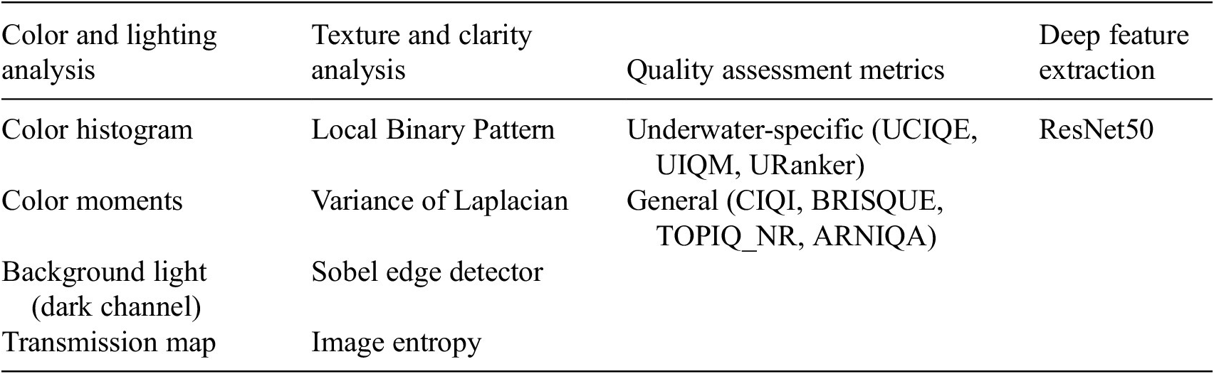


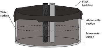

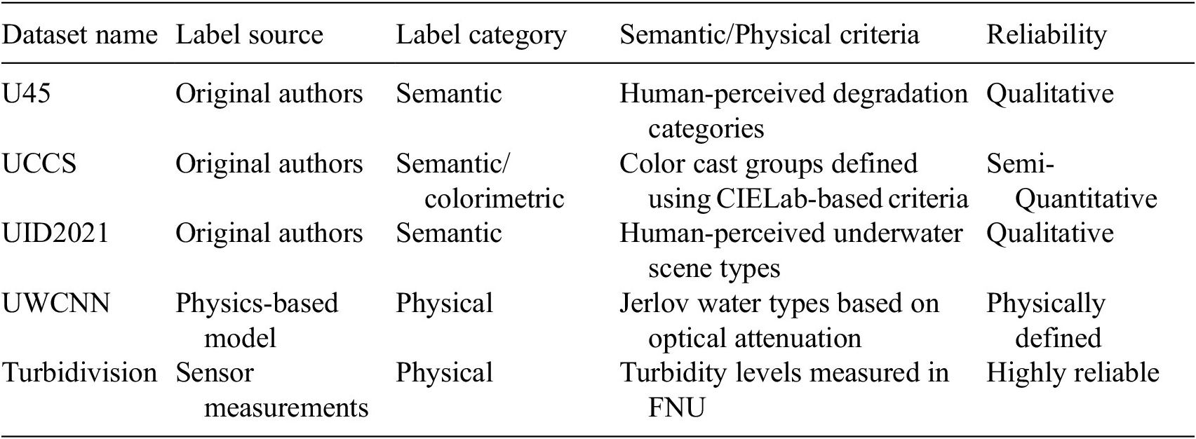


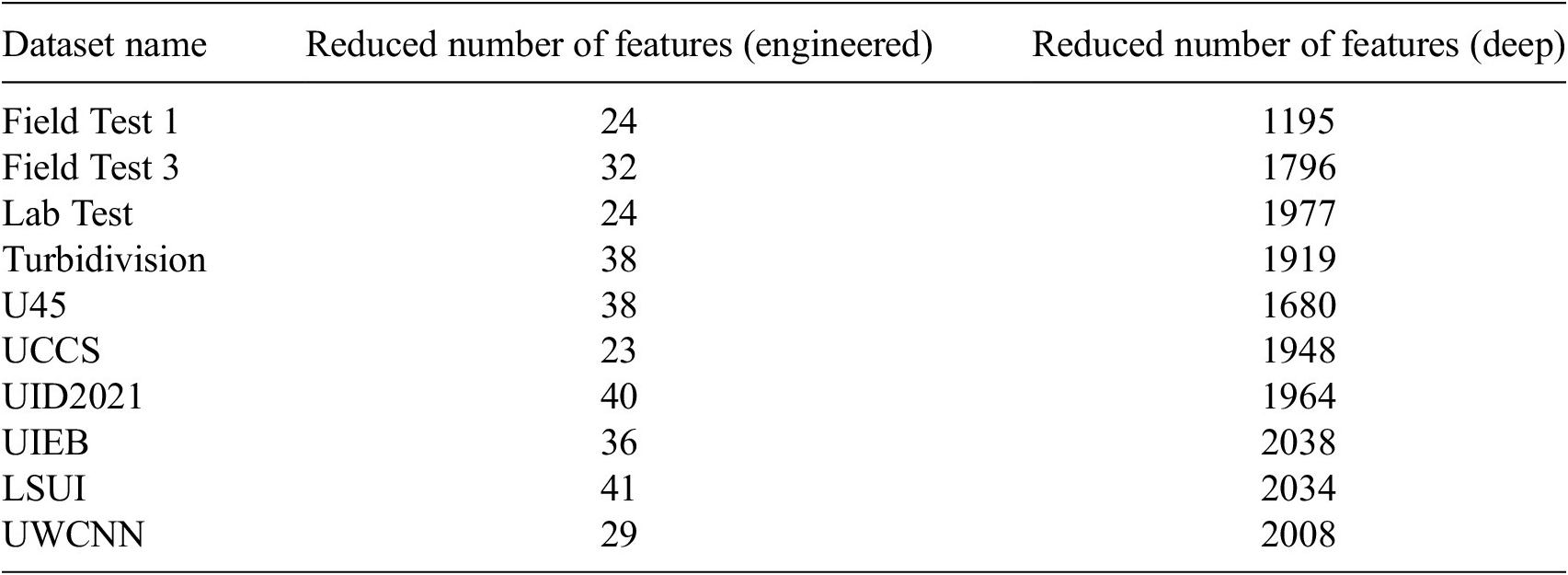
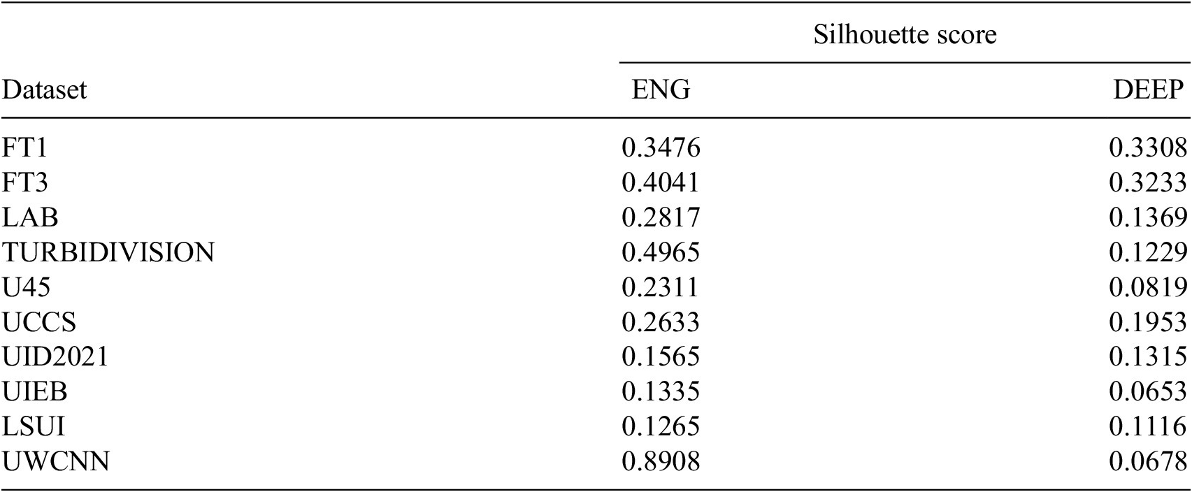


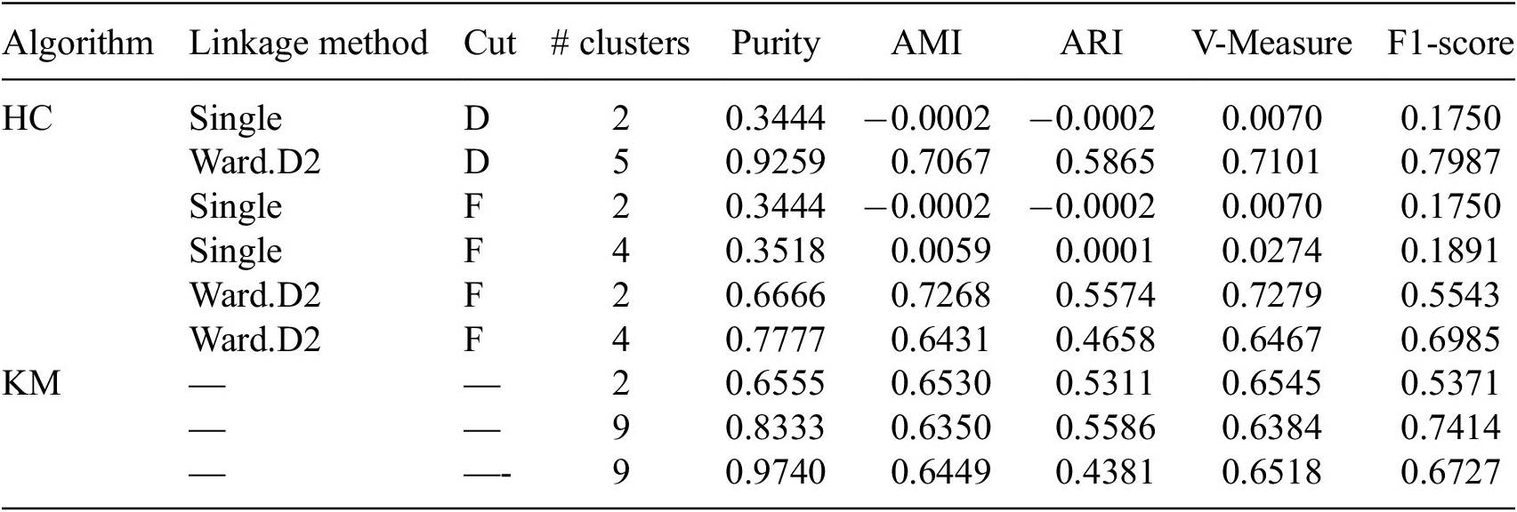

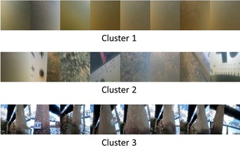
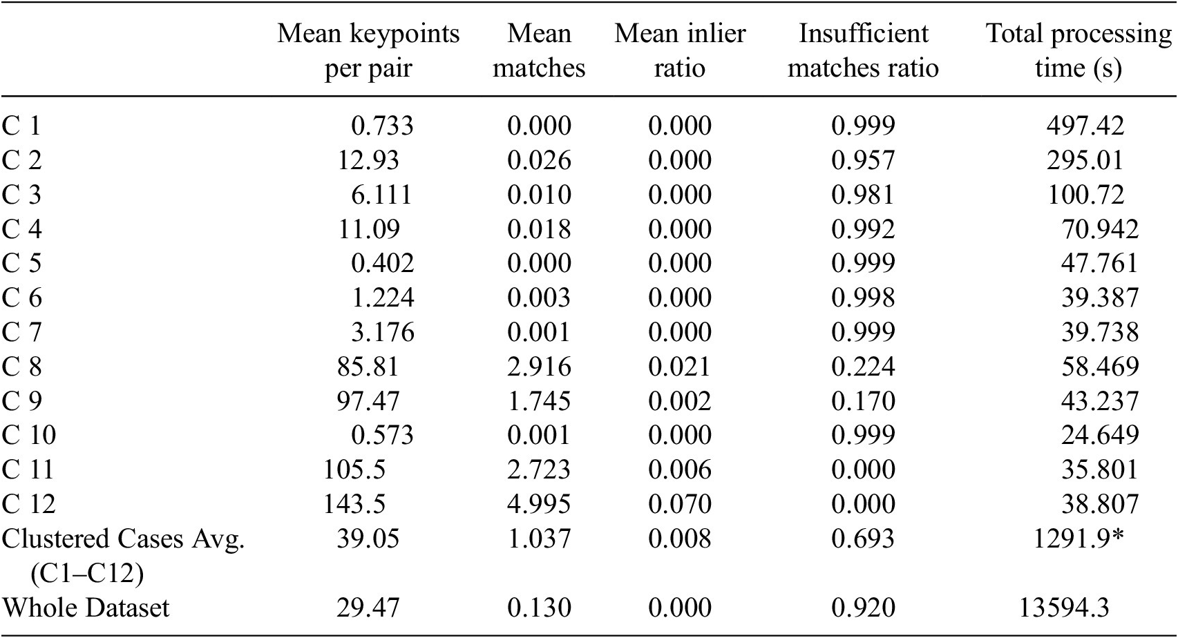
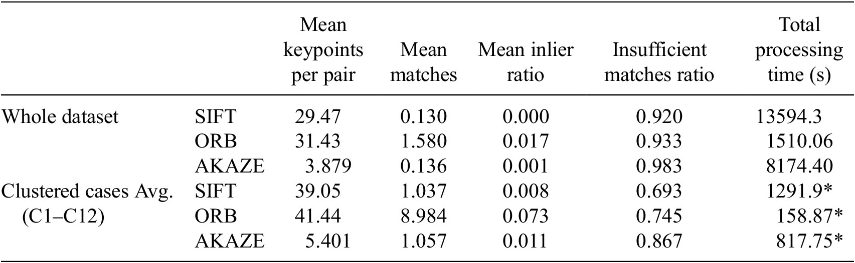
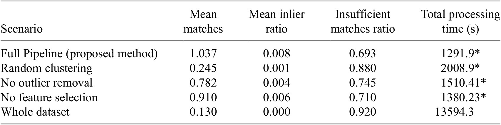
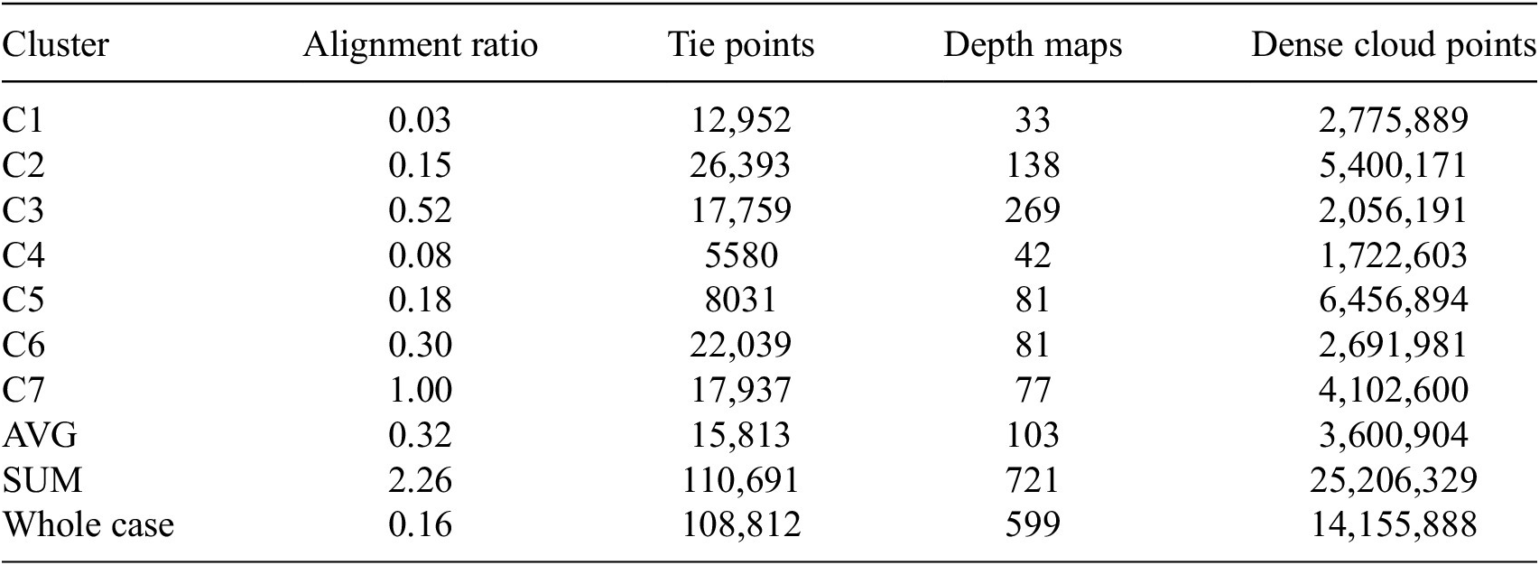

 Open access


Comments
No Comments have been published for this article.