Introduction

That the upper 100–200 m of large ice sheets are stratified in density is well known from many shallow-pit and deeper coring studies (e.g.Reference Gow Gow 1968; Reference Alley and BentleyAlley and Bentley 1988, this volume). It is also well known that the density contrast between layers remains sufficient to produce measurable radar reflections even from great depths (about 1000 m) and, in fact, density variations have been postulated as a dominant mechanism causing the long (hundreds of kilometers), continuous (on a scale of tens of meters) reflecting horizons that have been observed on radar data collected over all of the large ice sheets (Reference Paren and Robin.deParen and Robin 1975). Because of the suggestion that these layers may hold clues to present and past ice dynamics (Reference Whillans and JezekWhillans and Jezek 1987), much work has been done to elucidate the basic interaction between the deeper layers and the radar wave (Reference Bogorodsky, Bentley and GudmandsenBogorodsky and others 1986). Rather less attention has been paid to the upper 100 m of the ice sheet, in part because saturation limitations in the radar equipment precluded observations at shallow depths and in part because of the scientific focus of previous radar-sounding investigations. In this paper, we suggest that a different application of radar technology to ice-sheet research, namely radar altimetry, necessitates a more thorough investigation of near-surface effects. In radar altimetry, a radar apparatus is designed to measure very accurately the distance from the instrument’s platform to the surface of the Earth. Such radars were included as instruments aboard NASA’s Seasat and the U.S. Navy’s Geosat satellites and it is planned to carry them on future satellites, such as the European Remote Sensing Satellite. The essential information in radar altimetry is provided by the arrival time and the envelope of energy scattered solely from the surface of the ice sheet; sub-surface scattered energy is a potential contaminant. The precision of modern radar-to-surface measurements after processing is equivalent in range to about 10 cm (Reference TownsendTownsend 1980), which offers the tantalizing prospect of being able to discriminate subtle changes in ice-sheet shape (Reference ZwallyZwally 1984, 1986). But we wonder if, on this order of precision, other environmental effects may mask a change (or lack of change) in ice-sheet elevation. Specifically, in this paper we present a method that may help to answer the question of whether changes in stratification in the upper few meters of a glacier of constant shape can significantly perturb the envelope of a reflected radar pulse so as to simulate an apparent shift in ice-sheet topography.

Computational Method

We use a computational method described by Reference Jezek and ClayJezek and Clay (1984) for calculating the impulse response of a layered material. The approach is straightforward and somewhat more intuitive than others, such as the more common matrix formulations. It employs well-known theory for the reflection of a wave from a single layer overlying a half-space and then, followingReference Robinson and Treitel Robinson and Treitel (1980), obtaining the impulse response for a single layer by expressing the result in terms of z-transforms. Using a recursive solution for polynomial division, it is possible to calculate iteratively the response for an arbitrary number of layers. A band-limited result is obtained via convolution. In the following sketch of the technique, we explicitly invoke the following assumptions: smooth, horizontal layering; constant travel time through each layer; normally incident plane waves; non-dispersive media; that bulk absorption and volume scattering from individual ice grains are small.

The reflected amplitude of an electromagnetic wave at an interface is given by the well-known Fresnel equation

where e_l is the permittivity of the upper layer, e₂ is the permittivity of the lower layer and R₁₂ is the reflection coefficient for waves at the boundary between layer 1 and layer 2.

Now consider a short pulse incident on a single layer bounded on each side by semi-infinite media. Above the upper surface of the layer will be a series of upwardly traveling arrivals which have amplitudes

where Τ is the transmission coefficient, and the order of the subscripts indicates the direction of propagation across each interface. Now each term in the time sequence (2) is just the amplitude (a_n ) of an impulse arriving at a discrete time delay equal to the product of the integer n and the common time delay (∆t) throughout each layer. Hence we can write the time series as

δ(t) represents the amplitude function of the electric part (E) of the original incident impulse. The Fourier transform of (equ.3) is

Let

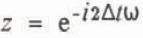
Then

Physically, z represents a unit time delay — the power of z gives the total time delay. Because the coefficients of z are less than unity, the right-hand side of (equ.6) sums to

R₁₃ represents the reflection coefficient of the layer and includes information on both the arrival time and the amplitude of all primary and multiple arrivals.

(equ.6) is the complete impulse response of a single layer covering a half-space. (equ.7) expresses the same result but as the ratio of two polynomials in z. For the case of many layers, one can start at the bottom layer, compute R _n−1,n and then use that result as the reflection coefficient for the bottom of the layer above. The computation proceeds until the top of the stack is reached.

The key to implementing this procedure on a computer is a recursive solution for the ratio of two polynomials:

The recursion formulae for the coefficients (c) of the solution are

By applying this algorithm to the quotient in (equ.7), we can calculate amplitudes of the primary reflection and all multiple reflections at the surface of the layer. Basically we retrieve (equ.6) and truncate the series at z^m where m is related to the maximum time of interest.

The power of this approach is demonstrated when there is more than one layer. In that case, the impulse response of the stack can be built up by starting with the layer at the bottom of the stack and working back up to the surface. For example, the impulse response (R₁₄ ) of two thin layers covering a half-space can be written

where R₁₂ is the reflection coefficient at the upper interface of the top layer and R₂₄ is the impulse response of the bottom thin layer.

Using (equ.6), (equ.12) can be written explicitly as

Application of the recursion relations yields

where ρ₀ is the first arrival from the top of the stack of layers and the succeeding terms represent primary and secondary reflections. An arbitrary number of additional layers can be modeled by an iterative application of this method.

Analysis

As a first case for study, we selected density data from a 2 m pit at Dome C, East Antarctica (personal communication from J. Bolzan) (Fig. 1). This is a relatively detailed depth-density profile, although there are probably more rapid density fluctuations that were not evident at the scale sampled (Reference PalaisPalais 1984).

Fig. 1.

Measured density (g/cm³) as a function of depth (cm) from a 2 m pit at Dome C, East Antarctica (personal communication from J. Bolzan). The profile was divided into 75 variable thickness layers, each of equal travel time.

Densities were converted to wave velocities using the empirical relationship (Reference Robin.de, Evans and BaileyRobin and others 1969)

where ρ is the relative density and n is the index of refraction. The results were used to divide the system into 75 layers, each with a 0.1 ns one-way travel time; consequently the thickness of each layer varied slightly. The impulse response of the measured profile was calculated; subsequently, each firn layer was successively replaced by an ice layer 1.7 cm thick (density 0.86 Mg/m³). The measured density of each firn layer was restored to its original value before proceeding to the next calculation. This model, although not particularly realistic for the central East Antarctic ice sheet, serves to illustrate the method and to provide some feel for the magnitude of effects in a situation where the local density profile does not vary by more than about 20% around the mean. We note that similar or thicker melt layers in otherwise dry firn do occur in large areas of Antarctica and Greenland and may be continuous over distances that are long when compared to the radar-altimeter footprint (e.g. Reference BensonBenson 1962,Reference Alley and Koci Alley and Koci 1988, Reference Mosley–Thompson, Thompson, Paskievitch and GrootesMosely-Thompson and others 1988). On the Siple Coast of West Antarctica, for example, melt features occur at about 50 year intervals, are often about 20 mm thick and require about 10 years to become buried to 2 m depth (Alley and Bentley 1988, this volume); thus the model used here represents possible conditions on the Siple Coast rather well.

Fig. 2.

Shape of the incident radar wave used in the calculation.

Synthetic waveforms were obtained by convolving the impulse response with a 20 ns long pulse modulated at 1 GHz and tapered at each end (Fig. 2). A long pulse was chosen to simulate heuristically the effects of surface roughness and volume scattering due to ice grains. (Sample Seasat waveforms shown inReference Martin, Zwally, Brenner and Bindschadler Martin and others (1983), and collected over Antarctica, are greater than 60 ns in width.)

Selected waveforms are shown in Figure 3 and reveal that the ice layer has a pronounced effect on the overall wave shape. The combination of constructive interference and multiple arrivals (the latter contributing energy that comprises a few per cent of the primary signal) can cause the part of the waveform affected by the ice layer to be almost 10 dB greater than when the ice layer is absent.

Fig. 3.

Selected waveforms derived from the convolution of the incident waveform (Fig. 2) and the impulse response of the measured density profile, interrupted by a single ice layer. The integers on the left indicate the number of the thin layer that contains the ice lens. Waveform 0 does not include an artificial ice layer.

When the ice layer is very near the surface, this causes the rising slope of the pulse to broaden; when the layer is deeper, the waveform exhibits a step-like change in amplitude.

To get some feeling for how the distortion in the waveform might affect the interpretation of travel time, two simple tracking schemes were developed. In each scheme, the amplitude in the generally flat part of the signal was measured. Then the half-amplitude point was located in the early part of the record. In the first method this was done automatically by searching the modulated waveform for the half-amplitude point. In the second method, the envelope of the waveform was sketched and the half-amplitude point was measured by eye. The same was done in the case where there was no ice layer and the difference time between the ice layer and ice-free cases was calculated. The results, shown in Figure 4, reveal an oscillating pattern of apparent two-way time delays that reach a maximum of about 4–5 ns. At layers deeper than interval 26, the step-like waveform clearly dominates, with the result that this simple tracking scheme is no longer meaningful. (Note that because the electrical properties of the layers are frequency-independent, the results can be scaled to other pulse-modulation frequencies. For example, the data can be interpreted as representing a 10 GHz pulse incident on a 20 cm stack of layers, giving rise to time delays of 0.4–0.5 ns. How Figure 4 would be modified due to a higher modulation frequency while using the 2 m stratigraphy remains to be calculated.)

Fig. 4.

Differences between the arrival time calculated for the case with an ice layer and the arrival time calculated for the case where there was no ice layer, as a function of the position of the ice layer in the stack. Abscissa labels are the layer number (roughly proportional to depth) into which the ice layer was inserted. Crosses indicate values computed automatically by finding the half-amplitude point of the modulated wave. Squares indicate values estimated by using the envelope of the waveforms.

Summary

With this simple example, we have attempted to show that density stratification can influence the interpretation of radar-altimetry data. On the one hand, this calculation is very primitive in that we neglected volume scattering from grains and the real effects of surface roughness. (Scattering coefficients given by Reference ZwallyZwally (1977) for grains 0.5 mm in radius, packed to a density of 0.48 g/cm³ and illuminated by 20 GHz radiation, yield attenuation rates of about 6 dB/m. Reference Ulaby, Moore and FungUlaby and others (1986, p. 1608) list penetration depths into snow (density 0.24 g/cm³, grain radii 0.5 mm and ambient temperature −1°C) of about 10 m at 13 GHz and greater than 100 m at 1 GHz.) In addition, the actual radar signal from satellite altimeters is transmitted as a very long chirp that is subsequently compressed in the radar electronics. (In the case of Seasat, the pulse was 3.2 µs long, with a 320 MHz bandwidth that was centered on 13.5 GHz (Townsend 1980).) Moreover, we ignore beamwidth effects and the fact that altimeters are designed to average over many successive pulses. On the other hand, our intuition is that by using a chirp we may introduce new complications (associated with the long, wide-bandwidth pulse) that further perturb the pulse shape. There is also independent evidence that buried ice layers are an important source of back-scatter, as reported by Reference Swift, Hayes, Herd, Jones and DelnoreSwift and others (1985), who studied Seasat scatterometer (14.6 GHz) and passive microwave-radiometer data collected over Greenland. Finally, on the basis of the ice-probing radar data noted in the Introduction and in core and pit studies, there is reason to believe that surface processes affecting ice-sheet morphology persist over great distances. If so, there may be systematic effects that, rather than being averaged out, are actually enhanced in the data. As such, we offer the following hypothesis: stratigraphy can affect the estimated arrival time of a radar pulse, and so variations in stratigraphy (production and/or burial of ice layers, for example) can cause variations in apparent ice-sheet elevation that has been deduced from repeated altimeter observations.

Acknowledgements

We thank W.F. Townsend and R.H. Thomas for many helpful suggestions.