1 Introduction
Near-inertial waves (NIWs) are inertia–gravity waves in rotating and stratified fluids with frequencies near the local inertial frequency,
 $f_{0}$
. In the oceans of Earth, an almost-universal strong density stratification means that NIWs have very small aspect ratios, large vertical shears and the lowest of internal wave frequencies. Partly because of their small aspect ratios and low frequencies, oceanic NIWs are generated by such diverse processes as fluctuating winds and flow over topography, contain roughly half of the total internal wave kinetic energy and are a main contributor to diapycnal mixing (Ferrari & Wunsch Reference Ferrari and Wunsch2009).
The weak dispersion and slow propagation of NIWs exposes them to strong interaction with balanced quasi-geostrophic (QG) flows. A basic introduction to NIW propagation through non-uniform balanced flows is given by the ray theories of Mooers (Reference Mooers1975) and Kunze (Reference Kunze1985), which show that near-inertial energy is attracted to regions of negative balanced vorticity and expelled from regions of positive vorticity. A more general theory valid both for ray-like NIW propagation and scattering by smaller-scale balanced flows was developed by Young & Jelloul (Reference Young and Ben Jelloul1997, YBJ hereafter). YBJ linearized the Boussinesq equations around a prescribed background flow and exploited weak near-inertial dispersion to develop a two-time asymptotic expansion that isolates the slow evolution of NIWs. The resulting YBJ NIW equation, which is similar to (1.8) below, describes the weakly dispersive propagation of
 $\unicode[STIX]{x1D6FD}$
-plane NIWs though advecting and refracting balanced flows of near-arbitrary spatial structure.
The YBJ NIW equation successfully describes many aspects of near-inertial propagation through realistic balanced flows (Klein & Smith Reference Klein and Smith2001; Klein, Smith & Lapeyre Reference Klein, Smith and Lapeyre2004; Danioux, Klein & Rivière Reference Danioux, Klein and Rivière2008), but ignores nonlinear finite-amplitude NIW dynamics and their corresponding feedback onto the balanced flow. In pursuit of a richer theory describing the coupled evolution of NIWs and balanced flows, Xie & Vanneste (Reference Xie and Vanneste2015, XV hereafter) derived a generalized-Lagrangian-mean model which joins the YBJ NIW equation to the QG equations. Like Bühler & McIntyre (Reference Bühler and McIntyre1998) and Wagner & Young (Reference Wagner and Young2015) and as in (1.7) below, in the XV model an NIW-induced balanced flow takes part in advecting QG potential vorticity and thus in the evolution of QG flow.
1.1 The
 $2f_{0}$
harmonic and motivation for a three-component model

Both YBJ and XV lack a conspicuous aspect of NIW evolution observed in the kinetic energy frequency spectra of the Ocean Storms Experiment (D’Asaro et al.
Reference D’Asaro, Eriksen, Levine, Paulson, Niiler and van Meurs1995), the observations of Niwa & Hibiya (Reference Niwa and Hibiya1999) and in the simulations of NIW–QG interaction by Danioux et al. (Reference Danioux, Klein and Rivière2008): the nonlinear generation of internal waves with frequency
 $2f_{0}$
. While these
 $2f_{0}$
waves have little horizontal kinetic energy relative to their parent NIWs, they can dominate pressure fields and contribute appreciably to vertical velocity fields and isopycnal displacements. Remarkably,
 $2f_{0}$
generation and subsequent horizontal radiation can remove energy from spatially compact regions of NIW–QG interaction, as discussed below and illustrated in figure 1. A primary motivation for this paper is the derivation of a more complete set of equations that contains the essential elements of YBJ and XV while including
 $2f_{0}$
waves. This derivation yields a model with three components: NIW velocity, balanced QG potential vorticity and the amplitude of the
 $2f_{0}$
pressure.
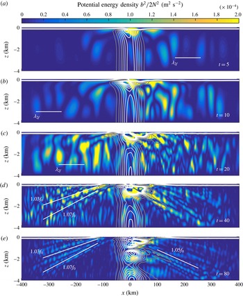
The numerical solution of a two-dimensional Boussinesq initial value problem involving the interaction between a barotropic jet and a surface-concentrated NIW. The shading shows the potential energy density
 $b^{2}/2N^{2}$
and the contours show the kinetic energy density at 10 levels between 0.01 and
 $0.1~\text{m}^{2}~\text{s}^{-2}$
at
 $t=5$
–
 $t=80$
inertial periods. The horizontal line on the
 $t=5$
, 10 and 20 snapshots shows the wavelength of a vertical mode-one
 $2f_{0}$
frequency internal wave. The slanting lines on the
 $t=40$
and
 $t=80$
snapshots show the characteristic propagation angles of NIWs with the indicated frequencies. The initial
 $v$
and
 $u$
are given in (1.1) and (1.2), where
 $V_{1}=0.4~\text{m}~\text{s}^{-1}$
,
 $L=40~\text{km}$
,
 $U=0.8~\text{m}~\text{s}^{-1}$
and
 $h=100~\text{m}$
. Only the central 800 km of a 1200 km computational domain is shown. The solution is relaxed to a surface-concentrated inertial oscillation in sponge layers 150 km thick on the edges of the domain.

To motivate the three-component model, we consider an initial value problem in the Boussinesq equations in which a surface-concentrated NIW interacts with a balanced barotropic jet in two dimensions
 $(x,z)$
. We use a constant inertial frequency
 $f_{0}=10^{-4}~\text{s}^{-1}$
and buoyancy frequency
 $N=2\times 10^{-3}~\text{s}^{-1}$
associated with a stable background buoyancy profile. The velocity field is
 $\boldsymbol{u}=u\hat{\boldsymbol{x}}+v\hat{\boldsymbol{y}}+w\hat{\boldsymbol{z}}$
and the dynamic buoyancy perturbation from the background is
 $b$
, so that the available potential energy density is
 $b^{2}/2N^{2}$
. The initial
 $v$
is a barotropic jet in geostrophic and hydrostatic balance flowing along the axis of
 $y$
, while the initial
 $u$
is a surface-concentrated, horizontally uniform and unbalanced flow which develops into an NIW. The balanced jet has the Gaussian profile
 $$\begin{eqnarray}v(x,z,0)=V_{0}+V_{1}\exp (-x^{2}/2L^{2}),\end{eqnarray}$$
where
 $V_{0}$
is defined so that
 $v(x,z,0)$
has zero horizontal average and thus no unbalanced component. The initial
 $u$
is horizontally uniform and concentrated in a layer of depth
 $h$
:
 $$\begin{eqnarray}u(x,z,0)=U_{0}\exp (-z^{2}/2h^{2}).\end{eqnarray}$$
The initial buoyancy
 $b$
and vertical velocity
 $w$
are zero. We solve this initial value problem in the Boussinesq equations using the spectral model of Winters, MacKinnon & Mills (Reference Winters, MacKinnon and Mills2004) with 1536 Fourier modes in
 $x$
and 768 sine/cosine modes in
 $z$
.
If the jet in (1.1) were not present, the initial condition in
 $u$
would develop into a horizontally uniform non-propagating perpetual inertial oscillation. Instead, refraction by the imposed jet injects small horizontal scales of size
 ${\sim}L$
into the NIW field, thus inducing near-inertial vertical propagation and catalysing radiation of low-mode
 $2f_{0}$
internal waves. The development of this process is illustrated in figure 1, which shows snapshots of the potential energy density at
 $t=5$
,
 $10$
,
 $20$
,
 $40$
and
 $80$
inertial periods. The kinetic energy density is indicated by 10 overlain contours between 0.01 and
 $0.1~\text{m}^{2}~\text{s}^{-2}$
. Throughout the simulation, the kinetic energy remains localized in the surface layer and in the near field of the barotropic jet. Bulges in the kinetic energy appearing at
 $t=20$
–
 $80$
inertial periods reveal the progress of vertical NIW propagation and show how NIW energy is refractively focused into the region of negative vorticity (Balmforth, Smith & Young Reference Balmforth, Smith and Young1998; Lee & Niiler Reference Lee and Niiler1998; Balmforth & Young Reference Balmforth and Young1999).
The vertical propagation of NIW kinetic energy is attended by an evolving potential energy field. Its most conspicuous aspect is a signal that extends for the full domain depth and radiates horizontally from the region of jet–NIW interaction. In the early stages, the potential energy signal has vertical mode-one structure. The horizontal line on the panels at
 $t=5$
, 10 and
 $20$
inertial periods indicates the horizontal wavelength
 $\unicode[STIX]{x1D706}_{2f}=2NH/\sqrt{3}f_{0}=92.4~\text{km}$
of a mode-one
 $2f_{0}$
frequency internal wave. Remarkably, while this
 $2f_{0}$
signal is generated by nonlinear NIW self-interaction in a small region, it rapidly radiates to fill a much larger volume without significant NIW activity (Danioux et al.
Reference Danioux, Klein and Rivière2008; Danioux & Klein Reference Danioux and Klein2008).
In addition to the low- and intermediate-mode
 $2f_{0}$
signal, narrow beams of potential energy radiate downwards and outwards from the centre of the domain. These beams are NIWs propagating at the characteristic angles indicated by the slanting lines on the snapshots at
 $t=40$
and
 $t=80$
inertial periods. The beams are produced by a scattering interaction between the surface-concentrated NIW and the jet. The rightward radiating beams are NIWs escaping the region of negative jet vorticity.
The two-dimensional NIW–jet interaction is thus characterized by at least three distinct phenomena: trapping of near-inertial energy in regions of negative balanced vorticity, beam-like radiation of near-inertial energy and emission of
 $2f_{0}$
waves. We use a multiple space- and time-scale expansion of the Boussinesq equations to construct a three-component model describing all of these processes.
1.2 Summary of the three-component model
In the three-component model, the horizontal velocity is
 $$\begin{eqnarray}u+\text{i}v\stackrel{\text{def}}{=}\text{e}^{-\text{i}f_{0}t}\,\text{L}\,A+(-\unicode[STIX]{x2202}_{y}+\text{i}\unicode[STIX]{x2202}_{x})\unicode[STIX]{x1D713}+\cdots \,,\end{eqnarray}$$
where
 $A(x,y,z,t)$
is the NIW envelope and
 $\unicode[STIX]{x1D713}(x,y,z,t)$
is the QG streamfunction. The differential operator
 $\text{L}$
in (1.3) is defined below in (1.7), and the dots on the right-hand side of (1.3) stand for additional contributions to the horizontal velocity: NIW harmonics, Stokes corrections and ageostrophic flow. The pressure field is
 $$\begin{eqnarray}p=f_{0}\unicode[STIX]{x1D713}+\frac{\text{i}f_{0}}{2}[\text{e}^{-\text{i}f_{0}t}(\unicode[STIX]{x2202}_{x}-\text{i}\unicode[STIX]{x2202}_{y})A+\text{e}^{-2\text{i}f_{0}t}2B]+\text{c.c.}+\cdots ,\end{eqnarray}$$
where
 $B(x,y,z,t)$
is the
 $2f_{0}$
wave envelope, ‘
 $\text{c.c.}$
’ stands for ‘complex conjugate’ and the dots indicate unimportant high-order corrections. The vertical velocity
 $w$
is
 $$\begin{eqnarray}w=-\frac{f_{0}^{2}}{2N^{2}}[\text{e}^{-\text{i}f_{0}t}(\unicode[STIX]{x2202}_{x}-\text{i}\unicode[STIX]{x2202}_{y})A_{z}+\text{e}^{-2\text{i}f_{0}t}4B_{z}]+\text{c.c.}\end{eqnarray}$$
The
 $2f_{0}$
contribution in
 $B$
features prominently in the vertical velocity field, despite its small contribution to the horizontal velocity.
The system consists of three equations: a wave-averaged QG potential vorticity equation, the NIW equation and a ‘
 $2f_{0}$
equation’ governing the evolution of
 $2f_{0}$
waves. The wave-averaged potential vorticity equation is
 $$\begin{eqnarray}q_{t}+\text{J}(\unicode[STIX]{x1D713},q)=0,\end{eqnarray}$$
where the potential vorticity is
 $$\begin{eqnarray}q=(\underbrace{\vphantom{\frac{f_{0}^{2}}{N^{2}}}\unicode[STIX]{x2202}_{x}^{2}+\unicode[STIX]{x2202}_{y}^{2}}_{\stackrel{\text{def}}{=}\unicode[STIX]{x0394}}+\underbrace{\unicode[STIX]{x2202}_{z}\frac{f_{0}^{2}}{N^{2}}\unicode[STIX]{x2202}_{z}}_{\stackrel{\text{def}}{=}\text{L}})\unicode[STIX]{x1D713}+\unicode[STIX]{x1D6FD}y+\frac{\text{i}}{2f_{0}}\text{J}(\text{L}A^{\ast },\text{L}A)+\frac{1}{4f_{0}}\unicode[STIX]{x0394}|\text{L}A|^{2}.\end{eqnarray}$$
In (1.6) and (1.7) the operator
 $\text{J}(a,b)=a_{x}b_{y}-a_{y}b_{x}$
is the Jacobian, the inertial of Coriolis frequency is
 $f=f_{0}+\unicode[STIX]{x1D6FD}y$
and
 $N(z)$
is the depth-dependent buoyancy frequency associated with strong background stratification. The two rightmost terms in (1.7) are quadratic NIW contributions to the wave-averaged potential vorticity. We assume that the
 $2f_{0}$
waves are too weak to contribute appreciably to the potential vorticity. The evolution of the NIW field is described by a generalization of the YBJ equation,
 $$\begin{eqnarray}\text{L}\,A_{t}+{\displaystyle \frac{\text{i}}{2}}f_{0}\unicode[STIX]{x0394}A+\text{J}(\unicode[STIX]{x1D713},\text{L}\,A)+\text{i}\text{L}\,A\left(\frac{1}{2}\unicode[STIX]{x0394}\unicode[STIX]{x1D713}+\unicode[STIX]{x1D6FD}y\right)+\frac{1}{2}\text{L}\,A^{\ast }(\unicode[STIX]{x2202}_{x}+\text{i}\unicode[STIX]{x2202}_{y})^{2}B=0.\end{eqnarray}$$
Equation (1.8) accounts for NIW dispersion and group propagation, horizontal advection by balanced flows, refraction by balanced flows and non-uniform planetary vorticity, and nonlinear NIW–
 $2f_{0}$
interaction. The NIW–
 $2f_{0}$
interaction term on the right end of (1.8) is identical to the term introduced by Young, Tsang & Balmforth (Reference Young, Tsang and Balmforth2008) into the YBJ equation to analyse near-inertial parametric subharmonic instability (PSI); in that work, the NIW–
 $2f_{0}$
interaction was implicated in the production of very small NIW vertical scales.
The evolution of the
 $2f_{0}$
amplitude
 $B$
is described by
 $$\begin{eqnarray}(\unicode[STIX]{x0394}+13\text{L})B_{t}+4\text{i}f_{0}(\unicode[STIX]{x0394}-3\text{L})B=-{\textstyle \frac{3}{2}}(\unicode[STIX]{x2202}_{x}-\text{i}\unicode[STIX]{x2202}_{y})^{2}(\text{L}\,A)^{2}.\end{eqnarray}$$
Equation (1.9) describes dispersion and propagation of
 $2f_{0}$
waves and energy transfer from NIWs via the source term on the right.
The three-component model, comprising (1.6)–(1.9), describes the coupled evolution of NIWs, QG flow and near-
 $2f_{0}$
internal waves. Like the XV system, the three-component model conserves two integral quantities: ‘wave action’ and ‘coupled energy’. The wave action is the sum of the NIW kinetic energy and the total energy of freely propagating near-
 $2f_{0}$
waves. The coupled energy is the sum of the total balanced energy, the near-inertial potential energy, an NIW–
 $\unicode[STIX]{x1D6FD}$
interaction term and terms associated with the NIW–
 $2f_{0}$
interaction.
A striking implication of both the XV and the three-component models is that NIWs can extract energy from balanced QG flow. This follows from the separation of two conservation laws for wave action and coupled energy, which together imply that an increase in NIW potential energy during NIW–flow interaction comes at the expense of balanced energy. Balanced flow thus loses energy when interacting with NIWs that consist almost entirely of kinetic energy, and NIW–QG interaction forms a link between large-scale balanced energy, the energy contained in the internal wave field, and wave breaking and diapycnal mixing. XV refer to this wave–mean interaction as ‘stimulated loss of balance’ to distinguish it from spontaneous loss of balance (Vanneste Reference Vanneste2013), emphasizing that it requires externally forced waves to ‘stimulate’ further production of wave energy at the expense of balanced energy. Unlike spontaneous wave generation, stimulated wave generation is a potentially significant energy sink for nearly balanced flows with small Rossby numbers.
Next, in § 2, we introduce the Boussinesq equations and special scaling assumptions, and define the multiple time and multiple vertical scales required to meet solvability conditions in the asymptotic derivation. In § 3 we expand the Boussinesq equations in wave amplitude, deriving the NIW equation as well as the
 $2f_{0}$
equation governing the evolution of the
 $2f_{0}$
harmonic. In § 4 we apply the wave-averaged contribution to the QG potential vorticity found by Wagner & Young (Reference Wagner and Young2015) to the near-inertial case. In § 5 we heuristically revise the formal theory derived in §§ 3 and 4 to arrive at the implementable model of (1.6)–(1.9). In § 6 we derive two conserved integral quantities from (1.6)–(1.9). In § 7 we compare numerical solutions of a two-dimensional initial value problem in both Boussinesq and three-component models, and in § 8 we assess the physical implications of the solutions. We conclude with a discussion of the significance and implications of the model in § 9.
2 The Boussinesq equations
We use the Boussinesq approximation by defining a constant reference density
 $\unicode[STIX]{x1D70C}_{0}$
and decomposing the total density into
 $$\begin{eqnarray}\unicode[STIX]{x1D70C}(\boldsymbol{x},t)=\unicode[STIX]{x1D70C}_{0}\left[1+g^{-1}\int _{z}^{0}N^{2}(z^{\prime })\,\text{d}z^{\prime }-g^{-1}b(\boldsymbol{x},t)\right],\end{eqnarray}$$
where
 $\boldsymbol{x}=(x,y,z)$
is position and
 $t$
is time. In (2.1), the resting buoyancy profile is the vertical integral of the buoyancy frequency
 $N^{2}(z)$
, and
 $b(\boldsymbol{x},t)$
is the dynamic buoyancy perturbation from background. Pressure is decomposed similarly into
 $-\unicode[STIX]{x1D70C}_{0}gz+\unicode[STIX]{x1D70C}_{0}P(z)+\unicode[STIX]{x1D70C}_{0}p(\boldsymbol{x},t)$
, where
 $P(z)$
is the resting hydrostatic pressure and the dynamic component of pressure is
 $\unicode[STIX]{x1D70C}_{0}p$
.
Using these definitions, the Boussinesq equations are
 $$\begin{eqnarray}\displaystyle & \displaystyle u_{t}+\boldsymbol{u}\boldsymbol{\cdot }\unicode[STIX]{x1D735}u-fv+p_{x}=0, & \displaystyle\end{eqnarray}$$
 $$\begin{eqnarray}\displaystyle & \displaystyle v_{t}+\boldsymbol{u}\boldsymbol{\cdot }\unicode[STIX]{x1D735}v+fu+p_{y}=0, & \displaystyle\end{eqnarray}$$
 $$\begin{eqnarray}\displaystyle & \displaystyle w_{t}+\boldsymbol{u}\boldsymbol{\cdot }\unicode[STIX]{x1D735}w+p_{z}=b, & \displaystyle\end{eqnarray}$$
 $$\begin{eqnarray}\displaystyle & \displaystyle b_{t}+\boldsymbol{u}\boldsymbol{\cdot }\unicode[STIX]{x1D735}b+wN^{2}=0, & \displaystyle\end{eqnarray}$$
 $$\begin{eqnarray}\displaystyle & \displaystyle u_{x}+v_{y}+w_{z}=0, & \displaystyle\end{eqnarray}$$
where
 $\boldsymbol{u}=u\hat{\boldsymbol{x}}+v\hat{\boldsymbol{y}}+w\hat{\boldsymbol{z}}$
is the fluid velocity. Subscripts with respect to
 $(x,y,z)$
or
 $t$
denote partial derivatives. We use the
 $\unicode[STIX]{x1D6FD}$
-plane approximation by introducing
 $f(y)=f_{0}+\unicode[STIX]{x1D6FD}y$
, where
 $f_{0}$
is the local inertial frequency and
 $\unicode[STIX]{x1D6FD}$
is its latitudinal variation.
2.1 Non-dimensionalization and scaling assumptions
We set the asymptotic reduction in motion by non-dimensionalizing the Boussinesq equations (2.2)–(2.6). We choose a spatial scaling that isolates NIWs at leading order and a velocity scaling that ensures that the back-rotated velocity and the QG potential vorticity share the same evolutionary time scale. Specifically, this requires that NIW dispersion acts on the same time scale as advection and refraction by the balanced flow. We use a single horizontal length scale,
 $L$
, and denote the scale of the near-inertial horizontal velocity with
 $\tilde{U}$
. The NIW ‘amplitude parameter’
 $$\begin{eqnarray}\unicode[STIX]{x1D716}\stackrel{\text{def}}{=}\frac{\tilde{U} }{f_{0}L}\end{eqnarray}$$
is crucial:
 $\unicode[STIX]{x1D716}\ll 1$
implies that nonlinear terms are small so that the NIW field is governed by linear dynamics to leading order.
The amplitude and importance of nonlinearity to balanced-flow evolution are measured by the Rossby number. We assume that the balanced flow is weak relative to the NIWs and that
 $\bar{U}=\unicode[STIX]{x1D716}\tilde{U}$
, where
 $\bar{U}$
is the characteristic velocity of the balanced flow. Under this scaling assumption the Rossby number is
 $$\begin{eqnarray}Ro\stackrel{\text{def}}{=}\frac{\bar{U}}{f_{0}L}=\unicode[STIX]{x1D716}^{2}.\end{eqnarray}$$
The NIW amplitude parameter and Rossby number have superficial similarity but different physical interpretations. The NIW amplitude can be interpreted as the ratio between the length scale
 $L$
and the radius of particle orbits in an inertial circle,
 $\tilde{U} /f_{0}$
. The Rossby number, on the other hand, is the ratio of the rotation time scale
 $1/f_{0}$
and advective time scale
 $L/\bar{U}=(\unicode[STIX]{x1D716}^{2}f_{0})^{-1}$
. The NIW envelope and the balanced flow co-evolve on the slow time scale
 $(\unicode[STIX]{x1D716}^{2}f_{0})^{-1}$
.
We denote the vertical scale of the NIWs by
 $\tilde{H}$
, and we use
 $\tilde{U}$
,
 $L$
and
 $\tilde{H}$
to non-dimensionalize the horizontal and vertical velocities,
 $$\begin{eqnarray}(u,v)=\tilde{U} \,({\check{u}},\check{v}),\quad w=\frac{\tilde{H}\tilde{U} }{L}\,\check{w},\end{eqnarray}$$
where non-dimensional variables are distinguished by
 $\check{\,}$
. Introducing
 $f_{0}$
, the local Coriolis or inertial frequency, and
 $N_{0}$
, the characteristic magnitude of
 $N(z)$
, we non-dimensionalize the buoyancy field with
 $$\begin{eqnarray}b=(\tilde{H}N_{0}^{2}\tilde{U} /f_{0}L)\,\check{b}.\end{eqnarray}$$
We adopt a geostrophic scaling for the pressure such that
 $$\begin{eqnarray}p=f_{0}L\bar{U}\check{p}=\unicode[STIX]{x1D716}f_{0}L\tilde{U} \check{p}.\end{eqnarray}$$
The inertial frequency is scaled so that
 $$\begin{eqnarray}\check{f}=1+\unicode[STIX]{x1D716}^{2}\check{\unicode[STIX]{x1D6FD}}\check{y},\end{eqnarray}$$
where
 $(x,y)=L(\check{x},\check{y})$
and
 $$\begin{eqnarray}\check{\unicode[STIX]{x1D6FD}}=\frac{\unicode[STIX]{x1D6FD}L^{2}}{\bar{U}}.\end{eqnarray}$$
Finally, we define an aspect ratio
 $$\begin{eqnarray}\unicode[STIX]{x1D6FC}\stackrel{\text{def}}{=}\unicode[STIX]{x1D716}\frac{N_{0}}{f_{0}}.\end{eqnarray}$$
By assuming
 $\unicode[STIX]{x1D6FC}=O(1)$
, we imply that
 $f_{0}/N_{0}=O(\unicode[STIX]{x1D716})$
and justify the hydrostatic approximation in the vertical momentum equation at all relevant orders in the perturbation theory.
2.2 Multiple scales: time and space
To describe both internal waves and slowly evolving balanced flow, we use the two-time method with a ‘fast’ time
 $\,\tilde{t}\,=f_{0}t$
and a ‘slow’ time
 $\bar{t}=\unicode[STIX]{x1D716}^{2}f_{0}t$
. Time derivatives are mapped according to
 $$\begin{eqnarray}\unicode[STIX]{x2202}_{t}\mapsto f_{0}(\unicode[STIX]{x2202}_{\,\tilde{t}\,}+\unicode[STIX]{x1D716}^{2}\unicode[STIX]{x2202}_{\bar{t}}).\end{eqnarray}$$
We use an Eulerian time average denoted with an overbar and defined as
 $$\begin{eqnarray}\bar{\unicode[STIX]{x1D719}}(\boldsymbol{x},\bar{t})\stackrel{\text{def}}{=}\frac{1}{T}\int _{t-T/2}^{t+T/2}\unicode[STIX]{x1D719}(\boldsymbol{x},t^{\prime })\,\text{d}t^{\prime },\quad \text{where}\quad \frac{1}{f_{0}}\ll T\ll \frac{L}{\bar{U}},\end{eqnarray}$$
to separate fast and slow flow components. Thus, any field
 $\unicode[STIX]{x1D719}$
can be represented as
 $$\begin{eqnarray}\unicode[STIX]{x1D719}=\bar{\unicode[STIX]{x1D719}}+\tilde{\unicode[STIX]{x1D719}},\end{eqnarray}$$
where
 $\bar{\unicode[STIX]{x1D719}}$
is the slowly evolving time-mean part and
 $\tilde{\unicode[STIX]{x1D719}}$
is the wavy part with
 $\overline{\tilde{\unicode[STIX]{x1D719}}}=0$
.
A multiple-vertical-scale expansion in the vertical is motivated by the disparity in aspect ratio between NIWs, and both observed
 $2f_{0}$
scales as well as standard QG flow. Denoting the vertical scale of the NIWs by
 $\tilde{H}$
, the internal wave dispersion relation implies that internal waves are near-inertial when the Burger number of the wave is small, or when
 $$\begin{eqnarray}\left(\frac{N_{0}\tilde{H}}{f_{0}L}\right)^{2}\ll 1.\end{eqnarray}$$
On the other hand, the standard QG equations assume that the Burger number of the balanced flow is of order unity. We use this requirement to define the vertical scale of the balanced flow,
 $\bar{H}$
, as
 $$\begin{eqnarray}\bar{H}\stackrel{\text{def}}{=}\frac{f_{0}L}{N_{0}}.\end{eqnarray}$$
We make the scaling assumption that
 $$\begin{eqnarray}\tilde{H}=\unicode[STIX]{x1D716}\bar{H}.\end{eqnarray}$$
This prescription for
 $\tilde{H}$
unifies the slow NIW dispersion time scale with the balanced-flow advection time scale. To capture both vertical scales in the expansion we split the vertical coordinate into a fast component,
 $\tilde{z}$
, and a slow component,
 $\bar{z}$
. Under this two-scale splitting, vertical derivatives become
 $$\begin{eqnarray}\unicode[STIX]{x2202}_{z}\mapsto \tilde{H}^{-1}(\unicode[STIX]{x2202}_{\tilde{z}}+\unicode[STIX]{x1D716}\,\unicode[STIX]{x2202}_{\bar{z}}).\end{eqnarray}$$
The vertical-scale splitting requires the introduction of a vertical average, which we define as
 $$\begin{eqnarray}\hat{\unicode[STIX]{x1D719}}=\frac{1}{H^{\prime }}\int _{\tilde{z}-H^{\prime }/2}^{\tilde{z}+H^{\prime }/2}\unicode[STIX]{x1D719}\,\,\text{d}\tilde{z}^{\prime },\quad \text{where }\tilde{H}\ll H^{\prime }\ll \bar{H}.\end{eqnarray}$$
The increase in complexity incurred by the multiple space-scale expansion is justified by a systematic explanation of the prominence and impact of the
 $2f_{0}$
harmonic on NIW evolution.
2.3 Complexifed non-dimensionalized equations
The derivation is greatly simplified by defining the complex horizontal coordinate and velocity field,
 $$\begin{eqnarray}s\stackrel{\text{def}}{=}x+\text{i}y\quad \text{and}\quad {\mathcal{U}}\stackrel{\text{def}}{=}u+\text{i}v.\end{eqnarray}$$
Spatial derivatives are expressed in terms of
 $s$
and
 $s^{\ast }$
via
 $$\begin{eqnarray}\unicode[STIX]{x2202}_{s}={\textstyle \frac{1}{2}}(\unicode[STIX]{x2202}_{x}-\text{i}\unicode[STIX]{x2202}_{y}),\quad \unicode[STIX]{x2202}_{s^{\ast }}={\textstyle \frac{1}{2}}(\unicode[STIX]{x2202}_{x}+\text{i}\unicode[STIX]{x2202}_{y}).\end{eqnarray}$$
These imply that
 $\unicode[STIX]{x0394}=4\unicode[STIX]{x2202}_{s}\unicode[STIX]{x2202}_{s^{\ast }}$
, and that
 $$\begin{eqnarray}u_{x}+v_{y}={\mathcal{U}}_{s}+{\mathcal{U}}_{s^{\ast }}^{\ast }\quad \text{and}\quad v_{x}-u_{y}=\text{i}\,{\mathcal{U}}_{s^{\ast }}^{\ast }-\text{i}\,{\mathcal{U}}_{s}.\end{eqnarray}$$
Using the scaling assumptions outlined above, and dropping decorations on non-dimensional variables, the complexified non-dimensional Boussinesq equations become
 $$\begin{eqnarray}\displaystyle & \displaystyle {\mathcal{U}}_{\,\tilde{t}\,}+\text{i}\,{\mathcal{U}}=-\unicode[STIX]{x1D716}(\boldsymbol{u}\boldsymbol{\cdot }\unicode[STIX]{x1D735}{\mathcal{U}}+2\,p_{s^{\ast }})-\unicode[STIX]{x1D716}^{2}({\mathcal{U}}_{\bar{t}}+w\,{\mathcal{U}}_{\bar{z}}+\text{i}\unicode[STIX]{x1D6FD}y\,{\mathcal{U}}), & \displaystyle\end{eqnarray}$$
 $$\begin{eqnarray}\displaystyle & \displaystyle p_{\tilde{z}}=\unicode[STIX]{x1D716}\,(b-p_{\bar{z}})-\unicode[STIX]{x1D716}^{2}\unicode[STIX]{x1D6FC}^{-2}[w_{\,\tilde{t}\,}+\unicode[STIX]{x1D716}(\boldsymbol{u}\boldsymbol{\cdot }\unicode[STIX]{x1D735}w)+\unicode[STIX]{x1D716}^{2}(ww_{\bar{z}}+w_{\bar{t}})], & \displaystyle\end{eqnarray}$$
 $$\begin{eqnarray}\displaystyle & \displaystyle b_{\,\tilde{t}\,}+wN^{2}=-\unicode[STIX]{x1D716}\,\boldsymbol{u}\boldsymbol{\cdot }\unicode[STIX]{x1D735}b-\unicode[STIX]{x1D716}^{2}(b_{\bar{t}}+wb_{\bar{z}}), & \displaystyle\end{eqnarray}$$
 $$\begin{eqnarray}\displaystyle & \displaystyle {\mathcal{U}}_{s}+{\mathcal{U}}_{s^{\ast }}^{\ast }+w_{\tilde{z}}=-\unicode[STIX]{x1D716}\,w_{\bar{z}}. & \displaystyle\end{eqnarray}$$
The bracketed terms in (2.27) are included for completeness, but never appear in the theory that follows. In terms of complex velocity the advection operators in (2.26) and (2.28) are
 $$\begin{eqnarray}\boldsymbol{u}\boldsymbol{\cdot }\unicode[STIX]{x1D735}={\mathcal{U}}\unicode[STIX]{x2202}_{s}+{\mathcal{U}}^{\ast }\unicode[STIX]{x2202}_{s^{\ast }}+w\unicode[STIX]{x2202}_{\tilde{z}}.\end{eqnarray}$$
The system in (2.26)–(2.29) is the basis for our asymptotic derivation.
3 The NIW equation
The NIW equation is derived by developing a perturbation expansion of (2.26)–(2.29) for
 $\unicode[STIX]{x1D716}\ll 1$
. We begin by expanding
 $\boldsymbol{u}$
,
 $b$
and
 $p$
each in a series in
 $\unicode[STIX]{x1D716}$
. For example, the complex velocity
 ${\mathcal{U}}$
has the expansion
 $$\begin{eqnarray}{\mathcal{U}}={\mathcal{U}}_{0}+\unicode[STIX]{x1D716}\,\,{\mathcal{U}}_{1}+\unicode[STIX]{x1D716}^{2}\,\,{\mathcal{U}}_{2}+\cdots .\end{eqnarray}$$
We develop (2.26)–(2.29) order by order in
 $\unicode[STIX]{x1D716}$
. For clarity, we express our results in dimensional variables, although the non-dimensional forms are indispensable for distinguishing each order in the development.
3.1 Leading order: NIWs
The leading-order terms in (2.26)–(2.29) are
 $$\begin{eqnarray}\displaystyle & \displaystyle {\mathcal{U}}_{0\,\tilde{t}\,}+\text{i}f_{0}\,{\mathcal{U}}_{0}=0, & \displaystyle\end{eqnarray}$$
 $$\begin{eqnarray}\displaystyle & \displaystyle p_{0\tilde{z}}=0, & \displaystyle\end{eqnarray}$$
 $$\begin{eqnarray}\displaystyle & \displaystyle b_{0\,\tilde{t}\,}+w_{0}N^{2}=0, & \displaystyle\end{eqnarray}$$
 $$\begin{eqnarray}\displaystyle & \displaystyle {\mathcal{U}}_{0s}+{\mathcal{U}}_{0s^{\ast }}^{\ast }+w_{0\tilde{z}}=0. & \displaystyle\end{eqnarray}$$
We write the solution to the horizontal momentum equation (3.2) in terms of an NIW envelope
 $M$
or
 $A$
,
 $$\begin{eqnarray}{\mathcal{U}}_{0}=\text{e}^{-\text{i}f_{0}\,\tilde{t}\,}\,M_{\tilde{z}}=\text{e}^{-\text{i}f_{0}\,\tilde{t}\,}\,\tilde{\text{L}}A,\end{eqnarray}$$
where
 $\tilde{\text{L}}$
is a second-order differential operator,
 $$\begin{eqnarray}\tilde{\text{L}}\stackrel{\text{def}}{=}\unicode[STIX]{x2202}_{\tilde{z}}\left(\frac{f_{0}^{2}}{N^{2}}\unicode[STIX]{x2202}_{\tilde{z}}\right).\end{eqnarray}$$
Both
 $A(x,y,\tilde{z},\bar{z},\bar{t})$
and
 $M=(f_{0}^{2}/N^{2})A_{\tilde{z}}$
prove useful for confronting the algebra that ensues. The representation in (3.6) ensures that the leading-order horizontal velocity is inertial over short times; small deviations in wave field frequency from
 $f_{0}$
are captured by the dependence of
 $M$
or
 $A$
on the slow time
 $\bar{t}$
. The construction in (3.6) also implies that the vertical average of the NIW horizontal velocity is zero at this order.
With the representation in (3.6), we can integrate the continuity equation (3.5) over the fast vertical coordinate
 $\tilde{z}$
to yield
 $$\begin{eqnarray}w_{0}=-\text{e}^{-\text{i}f_{0}\,\tilde{t}\,}M_{s}-\text{e}^{\text{i}f_{0}\,\tilde{t}\,}M_{s^{\ast }}^{\ast }+{\hat{w}}_{0},\end{eqnarray}$$
where the
 $\tilde{z}$
-independent function of integration
 ${\hat{w}}_{0}(x,y,\bar{z},\,\tilde{t}\,,\bar{t})$
is necessary to ensure solvability of the perturbation expansion at next order. If
 ${\hat{w}}_{0}$
is not included in (3.8), then the
 $O(\unicode[STIX]{x1D716})$
velocity field cannot satisfy continuity and the boundary conditions. At
 $O(\unicode[STIX]{x1D716})$
in (2.26)–(2.29), we find that
 ${\hat{w}}_{0}$
oscillates on the fast time scale with frequency
 $2f_{0}$
and is forced nonlinearly by NIW horizontal self-advection.
The leading-order buoyancy
 $b_{0}$
follows from integration of the buoyancy equation (3.4) using
 $w_{0}$
in (3.8),
 $$\begin{eqnarray}b_{0}=\text{i}f_{0}(\text{e}^{-\text{i}f_{0}\,\tilde{t}\,}A_{\tilde{z}s}-\text{e}^{\text{i}f_{0}\,\tilde{t}\,}A_{\tilde{z}s^{\ast }}^{\ast })+\hat{b}_{0},\end{eqnarray}$$
where as in (3.8) we include the function of integration
 $\hat{b}_{0}(x,y,\bar{z},\,\tilde{t}\,,\bar{t})$
. The vertical momentum equation (3.3) implies that the leading-order pressure
 $p_{0}$
does not depend on the fast vertical scale
 $\tilde{z}$
, or that
 $$\begin{eqnarray}p_{0}=\hat{p}_{0}.\end{eqnarray}$$
The leading-order pressure
 $p_{0}$
is eventually determined by (3.28) and (3.29) below and oscillates on a fast time scale with frequency
 $2f_{0}$
. An important feature eventually revealed by this expansion is that the large-vertical-scale
 $2f_{0}$
fields
 ${\hat{w}}_{0}$
,
 $\hat{b}_{0}$
and
 $\hat{p}_{0}$
appear at leading order in (3.8), (3.9) and (3.28). The magnitudes of these
 $2f_{0}$
fields follow from the two assumptions that the
 $2f_{0}$
horizontal velocity and vertical scales are respectively
 $O(\unicode[STIX]{x1D716})$
and
 $O(\unicode[STIX]{x1D716}^{-1})$
compared with their near-inertial counterparts. This scaling produces a description of NIW–
 $2f_{0}$
interaction that neglects the complicating effect of the mean flow
 $\unicode[STIX]{x1D713}$
on
 $2f_{0}$
evolution.
3.2 First order: wave-averaged geostrophic balance and
$2f_{0}$
harmonic

The
 $O(\unicode[STIX]{x1D716})$
terms in (2.26)–(2.29) are
 $$\begin{eqnarray}\displaystyle & \displaystyle {\mathcal{U}}_{1\,\tilde{t}\,}+\text{i}f_{0}\,{\mathcal{U}}_{1}=-2p_{0s^{\ast }}-\boldsymbol{u}_{0}\boldsymbol{\cdot }\unicode[STIX]{x1D735}{\mathcal{U}}_{0}, & \displaystyle\end{eqnarray}$$
 $$\begin{eqnarray}\displaystyle & \displaystyle p_{1\tilde{z}}=b_{0}-p_{0\bar{z}}, & \displaystyle\end{eqnarray}$$
 $$\begin{eqnarray}\displaystyle & \displaystyle b_{1\,\tilde{t}\,}+w_{1}N^{2}=-\boldsymbol{u}_{0}\boldsymbol{\cdot }\unicode[STIX]{x1D735}b_{0}, & \displaystyle\end{eqnarray}$$
 $$\begin{eqnarray}\displaystyle & \displaystyle {\mathcal{U}}_{1s}+{\mathcal{U}}_{1s^{\ast }}^{\ast }+w_{1\tilde{z}}=-w_{0\bar{z}}. & \displaystyle\end{eqnarray}$$
These equations describe wave-averaged geostrophic balance and the nonlinearly forced
 $2f_{0}$
harmonic.
3.2.1 Wave-averaged geostrophic balance
The time average of (3.11)–(3.14) yields the wave-averaged geostrophic balance conditions. These balance conditions are similar to those in Wagner & Young (Reference Wagner and Young2015) except that the restriction to NIWs means that there is no Stokes pressure contribution. We show this explicitly by first noting that the nonlinear term on the right-hand side of (3.11) is
 $$\begin{eqnarray}\boldsymbol{u}_{0}\boldsymbol{\cdot }\unicode[STIX]{x1D735}{\mathcal{U}}_{0}={\mathcal{J}}_{0}+\text{e}^{-2\text{i}f_{0}\,\tilde{t}\,}{\mathcal{J}}_{2}+\text{e}^{-\text{i}f_{0}\,\tilde{t}\,}{\hat{w}}_{0}M_{\tilde{z}\tilde{z}},\end{eqnarray}$$
where
 ${\mathcal{J}}_{0}$
and
 ${\mathcal{J}}_{2}$
are Jacobians defined by
 $$\begin{eqnarray}{\mathcal{J}}_{0}\stackrel{\text{def}}{=}\frac{\unicode[STIX]{x2202}(M^{\ast },M_{\tilde{z}})}{\unicode[STIX]{x2202}(\tilde{z},s^{\ast })}\quad \text{and}\quad {\mathcal{J}}_{2}\stackrel{\text{def}}{=}\frac{\unicode[STIX]{x2202}(M,M_{\tilde{z}})}{\unicode[STIX]{x2202}(\tilde{z},s)}.\end{eqnarray}$$
Next, we observe that the horizontal and vertical Stokes drifts,
 ${\mathcal{U}}^{S}$
and
 $w^{S}$
, are defined by
 $$\begin{eqnarray}{\mathcal{U}}^{S}\stackrel{\text{def}}{=}\,\overline{\unicode[STIX]{x1D743}_{0}\boldsymbol{\cdot }\unicode[STIX]{x1D735}{\mathcal{U}}_{0}}\quad \text{and}\quad w^{S}\stackrel{\text{def}}{=}\,\overline{\unicode[STIX]{x1D743}_{0}\boldsymbol{\cdot }\unicode[STIX]{x1D735}w_{0}},\end{eqnarray}$$
where
 $\unicode[STIX]{x1D743}_{0}=\unicode[STIX]{x1D709}_{0}\hat{\boldsymbol{x}}+\unicode[STIX]{x1D702}_{0}\hat{\boldsymbol{y}}+\unicode[STIX]{x1D701}_{0}\hat{\boldsymbol{z}}$
is the wave particle displacement, defined via
 $\unicode[STIX]{x1D743}_{0\,\tilde{t}\,}=\boldsymbol{u}_{0}$
and
 $\bar{\unicode[STIX]{x1D743}}_{0}=0$
. A direct calculation shows that
 $$\begin{eqnarray}\text{i}f_{0}\,{\mathcal{U}}^{S}=\overline{\boldsymbol{u}_{0}\boldsymbol{\cdot }\unicode[STIX]{x1D735}{\mathcal{U}}_{0}}={\mathcal{J}}_{0}.\end{eqnarray}$$
A similar calculation for the vertical Stokes drift
 $w^{S}$
shows that
 $$\begin{eqnarray}\text{i}f_{0}w^{S}=\frac{\text{i}f_{0}}{N^{2}}\,\overline{\boldsymbol{u}_{0}\boldsymbol{\cdot }\unicode[STIX]{x1D735}b_{0}}={\mathcal{K}}_{0}^{\ast }-{\mathcal{K}}_{0},\end{eqnarray}$$
where
 ${\mathcal{K}}_{0}$
is the Jacobian
 $$\begin{eqnarray}{\mathcal{K}}_{0}\stackrel{\text{def}}{=}\frac{\unicode[STIX]{x2202}(M^{\ast },M_{s})}{\unicode[STIX]{x2202}(\tilde{z},s^{\ast })}.\end{eqnarray}$$
The identity
 ${\mathcal{J}}_{0s}+{\mathcal{J}}_{0s^{\ast }}^{\ast }+{\mathcal{K}}_{0z}^{\ast }-{\mathcal{K}}_{0z}=0$
implies that the three-dimensional Stokes velocity in (3.18) and (3.19) is non-divergent.
Defining the QG streamfunction as
 $$\begin{eqnarray}\unicode[STIX]{x1D713}\stackrel{\text{def}}{=}\frac{\bar{p}_{0}}{f_{0}},\end{eqnarray}$$
we use the expressions for the Stokes velocities in (3.18) and (3.19) to write the time averages of (3.11) and (3.13) as
 $$\begin{eqnarray}\displaystyle & \displaystyle \bar{{\mathcal{U}}}_{1}+{\mathcal{U}}^{S}=2\text{i}\unicode[STIX]{x1D713}_{s^{\ast }}, & \displaystyle\end{eqnarray}$$
 $$\begin{eqnarray}\displaystyle & \displaystyle \bar{w}_{1}+w^{S}=0. & \displaystyle\end{eqnarray}$$
Equation (3.22) is the wave-averaged geostrophic balance condition for QG flow evolution in a field of strong NIWs. This balance condition lacks the Stokes pressure correction term that appears in the more general balance condition expressed by (4.38) in Wagner & Young (Reference Wagner and Young2015). From the leading-order vertical momentum equations (3.3), the pressure
 $p_{0}$
, and therefore
 $\unicode[STIX]{x1D713}$
, does not depend on the fast vertical coordinate
 $\tilde{z}$
.
3.2.2 The
$2f_{0}$
harmonic

Using the two-time decomposition in (2.17), we write the wavy parts of the first-order equations (3.11), (3.12) and (3.14),
 $$\begin{eqnarray}\displaystyle & \displaystyle \tilde{{\mathcal{U}}}_{1\,\tilde{t}\,}+\text{i}f_{0}\,\tilde{{\mathcal{U}}}_{1}+2\tilde{p}_{0s^{\ast }}=-\text{e}^{-2\text{i}f_{0}\,\tilde{t}\,}{\mathcal{J}}_{2}-\text{e}^{-\text{i}f_{0}\,\tilde{t}\,}\,{\hat{w}}_{0}M_{\tilde{z}\tilde{z}}, & \displaystyle\end{eqnarray}$$
 $$\begin{eqnarray}\displaystyle & \displaystyle \tilde{p}_{1\tilde{z}}=\tilde{b}_{0}-\tilde{p}_{0\bar{z}}, & \displaystyle\end{eqnarray}$$
 $$\begin{eqnarray}\displaystyle & \displaystyle \hat{b}_{0\,\tilde{t}\,}+{\hat{w}}_{0}N^{2}=0, & \displaystyle\end{eqnarray}$$
 $$\begin{eqnarray}\displaystyle & \displaystyle \tilde{{\mathcal{U}}}_{1s}+\tilde{{\mathcal{U}}}_{1s^{\ast }}^{\ast }+\tilde{w}_{1\tilde{z}}=-\tilde{w}_{0\bar{z}}, & \displaystyle\end{eqnarray}$$
where with (3.26) we include the vertically averaged leading-order buoyancy equation. It is (3.26), rather than the wavy part of (3.13), that describes the part of the
 $2f_{0}$
buoyancy field with large vertical scale. It should be noted that the final term on the right-hand side of (3.24) is not resonant because
 ${\hat{w}}_{0}$
oscillates with
 $2f_{0}$
frequency.
The system in (3.24)–(3.27) provides a complete description of the
 $2f_{0}$
harmonic of the NIW field. Importantly, part of this
 $2f_{0}$
harmonic response does not depend on the fast vertical coordinate
 $\tilde{z}$
. To isolate the slowly vertically varying part of the
 $2f_{0}$
harmonic we average (3.24)–(3.27) over
 $\tilde{z}$
and wrangle the resulting system into a single equation. We leave the details to appendix A and note the final result. Using the notation
 $$\begin{eqnarray}\tilde{p}_{0}=\text{i}f_{0}[\text{e}^{-2\text{i}f_{0}\,\tilde{t}\,}B(x,y,\bar{z},\bar{t})-\text{e}^{2\text{i}f_{0}\,\tilde{t}\,}B^{\ast }(x,y,\bar{z},\bar{t})],\end{eqnarray}$$
we find that
 $B$
solves
 $$\begin{eqnarray}\displaystyle \text{i}f_{0}(\unicode[STIX]{x0394}-3\bar{\text{L}})B=-{\textstyle \frac{3}{2}}\unicode[STIX]{x2202}_{s}^{2}\,\widehat{M_{z}^{2}}. & & \displaystyle\end{eqnarray}$$
The operator
 $\bar{\text{L}}$
is a second-order differential operator analogous to
 $\tilde{\text{L}}$
but defined in terms of the slow vertical scale
 $\bar{z}$
,
 $$\begin{eqnarray}\bar{\text{L}}\,\stackrel{\text{def}}{=}\,\unicode[STIX]{x2202}_{\bar{z}}\frac{f_{0}^{2}}{N^{2}}\unicode[STIX]{x2202}_{\bar{z}}.\end{eqnarray}$$
The ‘
 $2f_{0}$
equation’ in (3.29) describes forced
 $2f_{0}$
oscillations with a much larger vertical scale than the near-inertial fields. Because of this vertical-scale discrepancy, the vertical velocity of the
 $2f_{0}$
harmonic appears alongside the NIW vertical velocity at leading order in (3.8). As it stands, however, (3.29) cannot describe freely propagating
 $2f_{0}$
waves and thus cannot describe the waves that produce the prominent potential energy signal in figure 1. We modify (3.29) heuristically in § 5 to describe the freely propagating parts of
 $B$
, which roughly satisfy the
 $2f_{0}$
dispersion relation and thus obey
 $\unicode[STIX]{x0394}B\approx 3\text{L}\,B$
.
Continuing with the derivation of the NIW evolution equation, we use the expression for
 $\tilde{p}_{0}$
in (3.28) to integrate (3.24) for
 $\tilde{{\mathcal{U}}}_{1}$
. The full
 ${\mathcal{U}}_{1}$
field is
 $$\begin{eqnarray}{\mathcal{U}}_{1}=2\text{i}\unicode[STIX]{x1D713}_{s^{\ast }}+\text{i}f_{0}^{-1}{\mathcal{J}}_{0}+\text{e}^{-2\text{i}f_{0}\,\tilde{t}\,}(2B_{s^{\ast }}-\text{i}f_{0}^{-1}{\mathcal{J}}_{2})+{\textstyle \frac{2}{3}}\text{e}^{2\text{i}f_{0}\,\tilde{t}\,}B_{s^{\ast }}^{\ast }+\cdots \,,\end{eqnarray}$$
where the dots indicate terms proportional to
 $\text{e}^{-3\text{i}f_{0}\,\tilde{t}\,}$
and
 $\text{e}^{\text{i}f_{0}\,\tilde{t}\,}$
. Finally, we find
 $p_{1}-\hat{p}_{1}$
by subtracting the vertical average from (3.25), using (3.9) and integrating in
 $\tilde{z}$
to find
 $$\begin{eqnarray}p_{1}-\hat{p}_{1}=\text{i}f_{0}(A_{s}\text{e}^{-\text{i}f_{0}\,\tilde{t}\,}-A_{s^{\ast }}^{\ast }\text{e}^{\text{i}f_{0}\,\tilde{t}\,}).\end{eqnarray}$$
We now have
 ${\mathcal{U}}_{1}$
,
 ${\hat{w}}_{0}$
and
 $p_{1}$
, and are ready to proceed to the second-order system.
3.3 Second order: an NIW amplitude evolution equation
The
 $O(\unicode[STIX]{x1D716}^{2})$
terms in the horizontal momentum equation (2.26) are
 $$\begin{eqnarray}{\mathcal{U}}_{2\,\tilde{t}\,}+\text{i}f_{0}\,{\mathcal{U}}_{2}=-\boldsymbol{u}_{0}\boldsymbol{\cdot }\unicode[STIX]{x1D735}{\mathcal{U}}_{1}-\boldsymbol{u}_{1}\boldsymbol{\cdot }\unicode[STIX]{x1D735}{\mathcal{U}}_{0}-{\mathcal{U}}_{0\bar{t}}-\text{i}\unicode[STIX]{x1D6FD}y\,{\mathcal{U}}_{0}-2p_{1s^{\ast }}-w_{0}\,{\mathcal{U}}_{0\bar{z}}.\end{eqnarray}$$
Here, we finally apply the solvability condition arising from the introduction of multiple time scales. The solvability condition prevents the disordering of terms that would result from secular growth in
 ${\mathcal{U}}_{2}$
: we isolate resonant forcing terms on the right of (3.33) and set them collectively to zero. The amplitude equation yielded by this procedure governs the dependence of the NIW envelope
 $A$
on the slow time
 $\bar{t}$
. We note that the vertical average of (3.33) has no resonant terms.
We construct the amplitude equation piece by piece, starting at the far-right end of (3.33) and proceeding to the left. The final term
 $w_{0}\,{\mathcal{U}}_{0\bar{z}}$
in (3.33) has no parts proportional to
 $\text{e}^{-\text{i}f_{0}\,\tilde{t}\,}$
and so does not contribute to the amplitude equation. The next three terms from the left side of (3.33) are
 $$\begin{eqnarray}{\mathcal{U}}_{0\bar{t}}+\text{i}\unicode[STIX]{x1D6FD}y\,{\mathcal{U}}_{0}+2\unicode[STIX]{x2202}_{s^{\ast }}(p_{1}-\hat{p}_{1})=\text{e}^{-\text{i}f_{0}\,\tilde{t}\,}(\tilde{\text{L}}A_{\bar{t}}+\text{i}\unicode[STIX]{x1D6FD}y\,\tilde{\text{L}}A+2\text{i}f_{0}A_{ss^{\ast }})+\text{NRT},\end{eqnarray}$$
where
 $\text{NRT}$
stands for ‘non-resonant terms’. Next in line is
 $$\begin{eqnarray}\displaystyle (\boldsymbol{u}_{1}\boldsymbol{\cdot }\unicode[STIX]{x1D735}){\mathcal{U}}_{0}=\text{e}^{-\text{i}f_{0}\,\tilde{t}\,}\left[\,2\text{i}\frac{\unicode[STIX]{x2202}(\unicode[STIX]{x1D713},M_{\tilde{z}})}{\unicode[STIX]{x2202}(s^{\ast },s)}-{\mathcal{U}}^{S}M_{\tilde{z}s}-{\mathcal{U}}^{S\ast }M_{\tilde{z}s^{\ast }}-w^{S}M_{\tilde{z}\tilde{z}}\right]+\text{NRT}. & & \displaystyle\end{eqnarray}$$
It should be noted that to find (3.35) we need only consider the time-mean velocity
 $\bar{\boldsymbol{u}}_{1}$
, since
 ${\mathcal{U}}_{0}$
is proportional to
 $\text{e}^{-\text{i}f_{0}\,\tilde{t}\,}$
. The first term on the right of (3.33), involving the zero-order advection of the first-order velocity, is the most complicated. Carefully compiling the terms, we find
 $$\begin{eqnarray}\displaystyle (\boldsymbol{u}_{0}\boldsymbol{\cdot }\unicode[STIX]{x1D735}){\mathcal{U}}_{1} & = & \displaystyle \text{e}^{-\text{i}f_{0}\,\tilde{t}\,}(M_{\tilde{z}}{\mathcal{U}}_{1s}-M_{s}{\mathcal{U}}_{1\tilde{z}})+\text{e}^{\text{i}f_{0}\,\tilde{t}\,}(M_{\tilde{z}}^{\ast }{\mathcal{U}}_{1s^{\ast }}-M_{s^{\ast }}^{\ast }{\mathcal{U}}_{1\tilde{z}})+{\hat{w}}_{0}{\mathcal{U}}_{1\tilde{z}},\end{eqnarray}$$
 $$\begin{eqnarray}\displaystyle & = & \displaystyle \text{e}^{-\text{i}f_{0}\,\tilde{t}\,}\left[\frac{\unicode[STIX]{x2202}(M,\bar{{\mathcal{U}}}_{1})}{\unicode[STIX]{x2202}(\tilde{z},s)}+\frac{\text{i}}{f_{0}}\frac{\unicode[STIX]{x2202}({\mathcal{J}}_{2},M^{\ast })}{\unicode[STIX]{x2202}(\tilde{z},s^{\ast })}+2M_{\tilde{z}}^{\ast }B_{s^{\ast }s^{\ast }}\right]+\text{NRT}.\end{eqnarray}$$
Adding (3.35) to (3.37) yields
 $$\begin{eqnarray}(\boldsymbol{u}_{1}\boldsymbol{\cdot }\unicode[STIX]{x1D735}){\mathcal{U}}_{0}+(\boldsymbol{u}_{0}\boldsymbol{\cdot }\unicode[STIX]{x1D735}){\mathcal{U}}_{1}=\text{e}^{-\text{i}f_{0}\,\tilde{t}\,}\left[2\text{i}\frac{\unicode[STIX]{x2202}(\unicode[STIX]{x1D713},M_{\tilde{z}})}{\unicode[STIX]{x2202}(s^{\ast },s)}+2\text{i}\unicode[STIX]{x1D713}_{ss^{\ast }}M_{\tilde{z}}+2M_{\tilde{z}}^{\ast }B_{s^{\ast }s^{\ast }}\right]+\text{NRT}.\end{eqnarray}$$
The absence of terms cubic in
 $M$
is a remarkable aspect of (3.38): all 16 cubic
 $M$
terms in (3.35) and (3.37) conspire in collective cancellation. This simplification was previously noted by Falkovich, Kuznetsov & Medvedev (Reference Falkovich, Kuznetsov and Medvedev1994) and Zeitlin, Reznik & Ben Jelloul (Reference Zeitlin, Reznik and Ben Jelloul2003), and is the reason why no cubic terms appear in XV.
It is thus notable that our expansion identifies a surviving ‘honorary’ cubic term, proportional to
 $M_{\tilde{z}}^{\ast }B_{s^{\ast }s^{\ast }}$
, in (3.38). This new term results from the interaction of NIWs with both forced and freely propagating
 $2f_{0}$
waves. The requirement for
 $2f_{0}$
fields arises when the first-order continuity equation (3.27) is averaged over the small NIW vertical scale: if the vertical average of
 ${\mathcal{U}}_{1s}+{\mathcal{U}}_{1s^{\ast }}^{\ast }$
is non-zero, for example, then continuity can only be satisfied if
 ${\mathcal{U}}_{1}$
is permitted its own independent evolution. This solvability issue is addressed by introducing the
 $2f_{0}$
fields
 ${\hat{w}}_{0}$
,
 $\hat{b}_{0}$
and
 $\hat{p}_{0}$
at leading order in (3.8) and (3.9). This is the non-obvious step that ultimately produces the new term in (3.38).
The amplitude equation is then obtained from the sum of (3.34) and (3.38). In Cartesian coordinates and in terms of
 $A$
, the amplitude equation is
 $$\begin{eqnarray}\tilde{\text{L}}A_{\bar{t}}+\frac{\text{i}f_{0}}{2}\unicode[STIX]{x0394}A+\text{J}(\unicode[STIX]{x1D713},\tilde{\text{L}}A)+\text{i}\,\tilde{\text{L}}A\left(\frac{1}{2}\unicode[STIX]{x0394}\unicode[STIX]{x1D713}+\unicode[STIX]{x1D6FD}y\right)+\frac{1}{2}\,\tilde{\text{L}}A^{\ast }(\unicode[STIX]{x2202}_{x}+\text{i}\unicode[STIX]{x2202}_{y})^{2}B=0.\end{eqnarray}$$
The amplitude equation (3.39) is the YBJ equation except for the final
 $2f_{0}$
interaction term on the left-hand side. The
 $2f_{0}$
interaction term is identical to the one found by Young et al. (Reference Young, Tsang and Balmforth2008) in their analysis of energy transfer from prescribed
 $2f_{0}$
motions to NIWs by PSI.
4 The NIW-averaged available potential vorticity
Wave-averaged QG flow is governed by a wave-averaged potential vorticity equation (Bühler & McIntyre Reference Bühler and McIntyre1998; Wagner & Young Reference Wagner and Young2015),
 $$\begin{eqnarray}q_{\bar{t}}+\text{J}(\unicode[STIX]{x1D713},q)=0,\end{eqnarray}$$
where
 $\unicode[STIX]{x1D713}$
is defined through the balance condition (3.22) and
 $q$
is the wave-averaged available potential vorticity. Wagner & Young (Reference Wagner and Young2015) give a number of expressions for
 $q$
. Here, we use
 $$\begin{eqnarray}q\stackrel{\text{def}}{=}(\unicode[STIX]{x0394}+\text{L})\unicode[STIX]{x1D713}+\unicode[STIX]{x1D6FD}y+\underbrace{\overline{\text{J}(u_{0},\unicode[STIX]{x1D709}_{0})}+\overline{\text{J}(v_{0},\unicode[STIX]{x1D702}_{0})}+f_{0}\overline{\text{J}(\unicode[STIX]{x1D709}_{0},\unicode[STIX]{x1D702}_{0})}+{\textstyle \frac{1}{2}}(\overline{\unicode[STIX]{x1D709}_{0i}\unicode[STIX]{x1D709}_{0j}})_{\!,ij}}_{\stackrel{\text{def}}{=}q^{w}}.\end{eqnarray}$$
In (4.2) we define the wave contribution to the available potential vorticity,
 $q^{w}$
, in terms of the leading-order wave particle displacement
 $\unicode[STIX]{x1D743}_{0}=\unicode[STIX]{x1D709}_{0}\hat{\boldsymbol{x}}+\unicode[STIX]{x1D702}_{0}\hat{\boldsymbol{y}}+\unicode[STIX]{x1D701}_{0}\hat{\boldsymbol{z}}$
defined through
 $\unicode[STIX]{x1D743}_{0\,\tilde{t}\,}=\boldsymbol{u}_{0}$
.
In the present multiple-scale theory,
 $\unicode[STIX]{x1D713}$
and
 $q$
are both time-averaged and vertically averaged quantities. Consistency then demands that
 $q^{w}$
in (4.2) be vertically averaged as well. With the leading-order wave expressions (3.6) and (3.8) and using
 $M$
, a bit of algebra leads to
 $$\begin{eqnarray}q^{w}=-{\displaystyle \frac{1}{f_{0}}}(M_{ss^{\ast }}^{\ast }M_{\tilde{z}\tilde{z}}-2M_{\tilde{z}s^{\ast }}M_{\tilde{z}s}^{\ast }+M_{ss^{\ast }}M_{\tilde{z}\tilde{z}}^{\ast }).\end{eqnarray}$$
This is the expression for
 $q^{w}$
found by XV.
We then take the vertical average of
 $q^{w}$
, which yields a number of representations via integration by parts in
 $\tilde{z}$
, such as
 $$\begin{eqnarray}\displaystyle \widehat{q^{w}} & = & \displaystyle -{\displaystyle \frac{1}{f_{0}}}(\widehat{M_{ss^{\ast }}^{\ast }M_{\tilde{z}\tilde{z}}}-2\widehat{M_{\tilde{z}s^{\ast }}M_{\tilde{z}s}^{\ast }}+\widehat{M_{ss^{\ast }}M_{\tilde{z}\tilde{z}}^{\ast }}),\end{eqnarray}$$
 $$\begin{eqnarray}\displaystyle & = & \displaystyle {\displaystyle \frac{\text{i}}{2f_{0}}}\widehat{\text{J}(M_{\tilde{z}}^{\ast },M_{\tilde{z}})}+{\displaystyle \frac{1}{4f_{0}}}\unicode[STIX]{x0394}\,\widehat{|M_{\tilde{z}}|^{2}}.\end{eqnarray}$$
We take the second form, in (4.5), which is the form needed to furnish the three-component model in (1.6)–(1.9) with a coupled wave–mean-energy conservation law.
5 Remodelling
The formally derived model comprising (3.39), (4.2), (4.5) and (3.29) is a first draft that we heuristically revise to obtain the simpler and well-posed system in (1.6)–(1.9). This remodelling addresses two concerns with the multiple-scale formulation. First, the multiple vertical scales and vertical averages in (4.5) and (3.29) complicate computations. Second, the
 $2f_{0}$
equation in (3.29) cannot be solved when the NIW field and its
 $2f_{0}$
harmonic interact resonantly, which occurs when the nonlinear forcing on the right-hand side of (3.29) has spectral components in the null space of the operator
 $\unicode[STIX]{x0394}-3\text{L}$
on the left.
To address the first concern we reconsolidate vertical scales and eliminate vertical averaging from equations (4.5) and (3.29). Although this modification admits spurious small vertical scales into
 $\unicode[STIX]{x1D713}$
and
 $B$
, these small-scale parts of
 $\unicode[STIX]{x1D713}$
and
 $B$
contain little energy due to the ‘self-averaging’ Helmholtzian inversions that determine
 $\unicode[STIX]{x1D713}$
and
 $B$
through (4.2) and (3.29). In particular, energy is transferred most effectively to
 $B$
at resonant or near-resonant spectral components of (3.29) and (5.3). These spectral components lie close to the
 $2f_{0}$
dispersion relation and have large vertical scale relative to NIWs.
After consolidation of scales and dismissal of vertical averages the potential vorticity is given in terms of
 $\unicode[STIX]{x1D713}$
and wave-averaged properties as
 $$\begin{eqnarray}q=(\unicode[STIX]{x0394}+\text{L})\unicode[STIX]{x1D713}+\frac{\text{i}}{2f_{0}}\text{J}(\text{L}A^{\ast },\text{L}A)+\frac{1}{4f_{0}}\unicode[STIX]{x0394}|\text{L}A|^{2},\end{eqnarray}$$
and the NIW equation is
 $$\begin{eqnarray}\text{L}\,A_{t}+{\displaystyle \frac{\text{i}}{2}}f_{0}\unicode[STIX]{x0394}A+\text{J}(\unicode[STIX]{x1D713},\text{L}\,A)+\text{i}\text{L}\,A\left(\frac{1}{2}\unicode[STIX]{x0394}\unicode[STIX]{x1D713}+\unicode[STIX]{x1D6FD}y\right)+{\displaystyle \frac{1}{2}}\text{L}\,A^{\ast }(\unicode[STIX]{x2202}_{x}+\text{i}\unicode[STIX]{x2202}_{y})^{2}B=0.\end{eqnarray}$$
In (5.2) above,
 $\text{L}=\unicode[STIX]{x2202}_{z}\,f_{0}^{2}/N^{2}\,\unicode[STIX]{x2202}_{z}$
is the operator originally defined in (1.7) in terms of the single vertical scale
 $z$
. The evolution of
 $q$
in (5.1) is governed by the potential vorticity equation in (1.6).
The second issue regarding the non-invertibility of
 $\unicode[STIX]{x0394}-3\text{L}$
and the description of freely propagating
 $2f_{0}$
waves is addressed by applying the map
 $\unicode[STIX]{x2202}_{t}\mapsto -2\text{i}f_{0}+\unicode[STIX]{x2202}_{\bar{t}}$
to (3.24)–(3.27) prior to deriving (3.29). This procedure installs a time derivative in the
 $2f_{0}$
evolution equation (3.29) and fixes its resonance problem. We leave the details for appendix A and report the resulting modified
 $2f_{0}$
equation:
 $$\begin{eqnarray}(\unicode[STIX]{x0394}+13\text{L})B_{t}+4\text{i}f_{0}(\unicode[STIX]{x0394}-3\text{L})B=-{\textstyle \frac{3}{2}}(\unicode[STIX]{x2202}_{x}-\text{i}\unicode[STIX]{x2202}_{y})^{2}(\text{L}\,A)^{2}.\end{eqnarray}$$
Non-dimensionalizing (5.3) in the manner of § 2.1 reveals that
 $(\unicode[STIX]{x0394}+13\text{L})B_{t}$
is
 $\unicode[STIX]{x1D716}^{2}$
smaller than the rest of (5.3). The small term
 $(\unicode[STIX]{x0394}+13\text{L})B_{t}$
becomes important under conditions of near resonance when
 $4\text{i}f_{0}(\unicode[STIX]{x0394}-3\text{L})B$
is relatively small.
The expansion of
 $\unicode[STIX]{x2202}_{t}$
used to derive (5.3) is an application of the ‘method of reconstitution’ (Roberts Reference Roberts1985). Reconstitution successfully improves many asymptotic expansions, including the Navier–Stokes equations. Here, reconstitution of
 $2f_{0}$
dynamics by addition of the high-order term
 $(\unicode[STIX]{x0394}+13\text{L})B_{t}$
empowers (5.3) to describe freely propagating
 $2f_{0}$
waves.
6 Conservation laws
Like XV, we find that the wave-averaged system (1.6)–(1.9) conserves two integral quantities, which we call ‘wave action’ and ‘coupled energy’.
6.1 Wave action
The first conservation law follows from the wave equations (1.8) and (1.9). We multiply (1.8) with
 $(1/2)\text{L}\,A^{\ast }$
, add the complex conjugate and integrate over the domain. Using the
 $2f_{0}$
equation (5.3), and a liberal application of integration by parts, we find
 $$\begin{eqnarray}\frac{\text{d}}{\text{d}t}\int \;{\displaystyle \frac{1}{2}}|\text{L}\,A|^{2}+{\displaystyle \frac{1}{6}}|\unicode[STIX]{x1D735}B|^{2}+{\displaystyle \frac{13f_{0}^{2}}{6N^{2}}}|B_{z}|^{2}\;\,\text{d}V=0.\end{eqnarray}$$
The appearance of the
 $B$
terms in this first conservation law is a consequence of the time derivative in the
 $2f_{0}$
equation (5.3) and corresponds to the total energy in the freely propagating part of the near-
 $2f_{0}$
wave field. The conservation law (6.1) thus implies that resonant generation of propagating
 $2f_{0}$
waves extracts near-inertial kinetic energy.
6.2 Coupled energy
The second conserved quantity is a wave–mean coupled energy. We derive the associated conservation law by multiplying the potential vorticity equation (4.1) with
 $\unicode[STIX]{x1D713}$
and integrating over the domain. The Jacobian term
 $\unicode[STIX]{x1D713}\,\text{J}(\unicode[STIX]{x1D713},q)$
can be written as an exact derivative and integrates to zero. Applying integration by parts, we are left with
 $$\begin{eqnarray}\frac{\text{d}\mathscr{E}_{\unicode[STIX]{x1D713}}}{\text{d}t}=\int \unicode[STIX]{x1D713}q_{t}^{w}\,\text{d}V,\end{eqnarray}$$
where
 $q^{w}$
is the wave potential vorticity defined in (4.2) and
 $$\begin{eqnarray}\mathscr{E}_{\unicode[STIX]{x1D713}}\stackrel{\text{def}}{=}\int \frac{1}{2}|\unicode[STIX]{x1D735}\unicode[STIX]{x1D713}|^{2}+\frac{1}{2}{\displaystyle \frac{f_{0}^{2}}{N^{2}}}\unicode[STIX]{x1D713}_{z}^{2}\;\,\text{d}V\end{eqnarray}$$
is the total balanced QG energy. Next, we multiply (1.8) by
 $\text{i}\text{L}\,A_{t}^{\ast }/2f_{0}$
, add the complex conjugate and integrate over the domain to obtain
 $$\begin{eqnarray}\frac{\text{d}\mathscr{E}_{f}}{\text{d}t}=-\int \unicode[STIX]{x1D713}q_{t}^{w}\,\text{d}V-{\displaystyle \frac{\text{i}}{2f_{0}}}\int B^{\ast }\unicode[STIX]{x2202}_{t}\unicode[STIX]{x2202}_{s}^{2}(\text{L}\,A)^{2}-B\unicode[STIX]{x2202}_{t}\unicode[STIX]{x2202}_{s^{\ast }}^{2}(\text{L}\,A^{\ast })^{2}\,\text{d}V,\end{eqnarray}$$
where
 $$\begin{eqnarray}\mathscr{E}_{f}\stackrel{\text{def}}{=}\int {\displaystyle \frac{f_{0}^{2}}{4N^{2}}}|\unicode[STIX]{x1D735}A_{z}|^{2}+{\displaystyle \frac{\unicode[STIX]{x1D6FD}y}{2f_{0}}}|\text{L}\,A|^{2}\;\,\text{d}V\end{eqnarray}$$
is the sum of the NIW potential energy and an action-like term associated with the
 $\unicode[STIX]{x1D6FD}$
-effect. The first term on the right of (6.4) corresponds to the term on the right of (6.2) and will cancel when these equations are added. Substitution of the
 $2f_{0}$
equation (1.9) and its complex conjugate into the second integral on the right of (6.4) followed by persistent integration by parts produces
 $$\begin{eqnarray}\frac{\text{d}\mathscr{E}_{2f}}{\text{d}t}={\displaystyle \frac{\text{i}}{2f_{0}}}\int B^{\ast }\unicode[STIX]{x2202}_{t}\unicode[STIX]{x2202}_{s}^{2}(\text{L}\,A)^{2}-B\,\unicode[STIX]{x2202}_{t}\unicode[STIX]{x2202}_{s^{\ast }}^{2}(\text{L}\,A^{\ast })^{2}\,\text{d}V,\end{eqnarray}$$
where
 $$\begin{eqnarray}\displaystyle \mathscr{E}_{2f} & \stackrel{\text{def}}{=} & \displaystyle \int {\displaystyle \frac{\text{i}}{12f_{0}}}[B(\unicode[STIX]{x0394}+13\text{L})B_{t}^{\ast }-B^{\ast }(\unicode[STIX]{x0394}+13\text{L})B_{t}]-{\displaystyle \frac{1}{3}}|\unicode[STIX]{x1D735}B|^{2}+{\displaystyle \frac{f_{0}^{2}}{N^{2}}}|B_{z}|^{2}\,\text{d}V,\end{eqnarray}$$
 $$\begin{eqnarray}\displaystyle & = & \displaystyle \int {\displaystyle \frac{\text{i}}{8f_{0}}}[B^{\ast }(\unicode[STIX]{x2202}_{x}-\text{i}\unicode[STIX]{x2202}_{y})^{2}(\text{L}\,A)^{2}-B(\unicode[STIX]{x2202}_{x}+\text{i}\unicode[STIX]{x2202}_{y})^{2}(\text{L}\,A^{\ast })^{2}]+{\displaystyle \frac{1}{3}}|\unicode[STIX]{x1D735}B|^{2}-{\displaystyle \frac{f_{0}^{2}}{N^{2}}}|B_{z}|^{2}\,\text{d}V.\qquad\end{eqnarray}$$
An additional substitution of (1.9) and its complex conjugate transforms equation (6.7) into (6.8). The conservation of coupled energy emerges from the combination of (6.2), (6.4) and (6.6),
 $$\begin{eqnarray}\frac{\text{d}}{\text{d}t}(\mathscr{E}_{\unicode[STIX]{x1D713}}+\mathscr{E}_{f}+\mathscr{E}_{2f})=0.\end{eqnarray}$$
The conservation law in (6.9) is identical to XV’s conservation law except for the addition of the
 $\mathscr{E}_{2f}$
term. Equation (6.9) is the analogue of a conservation law found by Danioux, Vanneste & Bühler (Reference Danioux, Vanneste and Bühler2015) that relates the evolution of NIW potential energy to advection and refraction by steady geostrophic flows.
A thought experiment due to XV illuminates an important implication of (6.9). Envision the rapid and stormy deposition of a horizontally extensive surface-concentrated current in a region of geostrophic turbulence. As the storm passes, the unbalanced current develops into a surface-concentrated NIW that is almost horizontally uniform, and therefore has little potential energy, and thus
 $\mathscr{E}_{f}\approx 0$
. Over subsequent inertial periods, NIW refraction and advection by the geostrophic flow drives the creation of near-inertial horizontal scales and potential energy, which leads to vertical propagation of a refracted NIW signal and the generation of
 $2f_{0}$
internal waves. Because the wave action in (6.1) and coupled energy in (6.9) are distinct and independent conservation laws, the total NIW and
 $2f_{0}$
wave energy increases in this process at the sole expense of energy in the geostrophic flow. The role of
 $\mathscr{E}_{2f}$
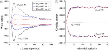
in (6.9) is unfortunately obscure in this thought experiment, although the diagnosis of (6.9) presented in figure 7 below shows that the effect is minor in some cases.
7 Comparison of the three-component model and the Boussinesq equations
To build confidence in the heuristic and asymptotic approximations used to develop the three-component model, we compare numerical solutions of a two-dimensional initial value problem in the three-component model and the Boussinesq equations. The initial problem is similar to that shown in figure 1, in which a surface-concentrated NIW interacts with a barotropic balanced velocity field. In addition to solutions intended for direct comparison, we compute solutions to a two-component model without
 $2f_{0}$
dynamics, and a three-component model with the PSI-like part of the NIW–
 $2f_{0}$
interaction removed. The physical implications of the numerical solutions are discussed in § 8.
7.1 A surface-concentrated NIW in random barotropic flow
The initial value problem involves the interaction of a surface-concentrated NIW with random barotropic balanced flow. The two-dimensional physical domain is bounded by rigid lids in
 $z$
with height
 $H=4$
km and is periodic in
 $x$
with width
 $L=800$
km. The stratification is uniform, with buoyancy frequency
 $N=2\times 10^{-3}~\text{s}^{-1}$
, and the inertial frequency is
 $f_{0}=10^{-4}\;\text{s}^{-1}=N/20$
, with
 $\unicode[STIX]{x1D6FD}=0$
. As for the problem considered in § 1, the NIW initial condition is
 $$\begin{eqnarray}\text{L}\,A(x,z,0)=u(x,z,0)=U_{0}\,\exp (-z^{2}/2h^{2}),\end{eqnarray}$$
with
 $h=100$
m. We consider initial NIW surface velocities of
 $U_{0}=0.4,0.2$
and
 $0.1~\text{m}~\text{s}^{-1}$
.
The initial balanced
 $v$
velocity is
 $$\begin{eqnarray}\unicode[STIX]{x1D713}_{x}(x,z,0)=v(x,z,0)=V_{0}\,\mathop{\sum }_{n=4}^{14}\left(\frac{k_{4}}{k_{n}}\right)^{2}\cos (k_{n}x+\unicode[STIX]{x1D719}_{n}),\end{eqnarray}$$
where
 $k_{n}\stackrel{\text{def}}{=}2\unicode[STIX]{x03C0}n/L$
and the
 $\unicode[STIX]{x1D719}_{n}$
are random phases between 0 and
 $2\unicode[STIX]{x03C0}$
for each component of the geostrophic flow. We choose
 $V_{0}=0.1~\text{m}~\text{s}^{-1}$
for all simulations. This produces a maximum velocity of
 $\max (v)\,\approx \,0.2~\text{m}~\text{s}^{-1}$
, a maximum Rossby number of
 $\max (v_{x})/f_{0}\,\approx \,0.1$
and a root-mean-square Rossby number of
 $\text{r.m.s.}(v_{x})/f_{0}\approx 0.05$
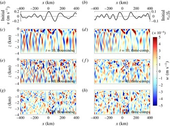
. The balanced flow and its associated vorticity field are plotted in figures 2(a,b)–4(a,b).
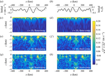
Comparison of wave speed in numerical solutions to the three-component and Boussinesq models. (a,b) The
 $x$
dependence of the initial balanced velocity
 $v$
(a) and the balanced vorticity normalized by
 $f_{0}$
,
 $v_{x}/f_{0}$
(b). (c–h) The wave speed defined in (7.8) at
 $t=10$
, 40 and 80 inertial periods in the Boussinesq model (c,e,g) and the three-component model (d,f,h). The initial NIW surface velocity is
 $U_{0}=0.4~\text{m}~\text{s}^{-1}$
.

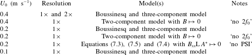
The numerical solutions we report are listed in table 1. We choose simulation parameters both for ease of numerical integration and for consistency with oceanic scenarios. In particular,
 $V_{0}=0.1~\text{m}~\text{s}^{-1}$
leads to ‘reasonable’ NIW vertical propagation in 10 or 20 inertial periods; smaller values of
 $V_{0}$
lead to slower vertical propagation. It should be noted, however, that
 $V_{0}=0.1~\text{m}~\text{s}^{-1}$
violates assumptions made in § 2 to justify the asymptotic derivation of the three-component model: the expansion assumes that
 $\bar{U}/\tilde{U} =\tilde{H}/\bar{H}=\unicode[STIX]{x1D716}\ll 1$
. In the following simulations,
 $\tilde{H}/\bar{H}=\unicode[STIX]{x03C0}h/H=0.08\ll 1$
while
 $\bar{U}/\tilde{U} =V_{0}/U_{0}$
ranges between
 $0.25$
and
 $1$
, so that the balanced flow seems to be too strong given that the non-dimensionalization in § 2.1 assumes
 $\tilde{H}/\bar{H}\sim \bar{U}/\tilde{U} =\unicode[STIX]{x1D716}\ll 1$
. Nevertheless, we find generally good agreement between the predictions of the three-component model and full Boussinesq solutions. Other calculations with
 $V_{0}$
reduced to
 $0.025~\text{m}~\text{s}^{-1}$
not shown here also validate the three-component model.
We note finally that that our two-dimensional computations do not test all aspects of the three-component model: with
 $\unicode[STIX]{x2202}_{y}=0$
the advective terms
 $\text{J}(\unicode[STIX]{x1D713},\text{L}\,A)$
and
 $\text{J}(\unicode[STIX]{x1D713},q)$
vanish and the available potential vorticity (Wagner & Young Reference Wagner and Young2015)
 $q$
does not evolve from its initial distribution. The two-dimensional simulations reported here are interesting primarily as a test of the nonlinear NIW–
 $2f$
interaction and the associated production of small vertical scales. Probing of the advective terms requires either three-dimensional solutions like those in Danioux et al. (Reference Danioux, Klein and Rivière2008) or solutions of the two-dimensional model introduced in § 6.2 of XV.




7.2 Methods
In two dimensions, the APV equation (1.6) reduces to
 $q_{t}=0$
and implies that
 $q$
is constant. We decompose the balanced streamfunction into
 $\unicode[STIX]{x1D713}(x,z,t)=\unicode[STIX]{x1D713}^{q}(x,z)+\unicode[STIX]{x1D713}^{w}(x,z,t)$
, where
 $$\begin{eqnarray}(\unicode[STIX]{x2202}_{x}^{2}+\text{L})\unicode[STIX]{x1D713}^{q}=q\quad \text{and}\quad (\unicode[STIX]{x2202}_{x}^{2}+\text{L})\unicode[STIX]{x1D713}^{w}=-\frac{1}{4f_{0}}\unicode[STIX]{x2202}_{x}^{2}|\text{L}\,A|^{2}.\end{eqnarray}$$
Like
 $q$
,
 $\unicode[STIX]{x1D713}^{q}$
is constant in time and is determined by the initial condition. Because
 $\text{L}\,A$
is initially uniform, we have
 $\unicode[STIX]{x1D713}^{q}=\unicode[STIX]{x1D713}(t=0)$
and thus
 $\unicode[STIX]{x1D713}_{xx}^{q}=v_{x}(t=0)$
. With this decomposition the two-dimensional three-component system becomes
 $$\begin{eqnarray}\displaystyle & \displaystyle \text{L}\,A_{t}+{\displaystyle \frac{\text{i}}{2}}f_{0}A_{xx}+{\displaystyle \frac{\text{i}}{2}}(\unicode[STIX]{x1D713}_{xx}^{q}+\unicode[STIX]{x1D713}_{xx}^{w})\text{L}\,A+\frac{1}{2}B_{xx}\text{L}\,A^{\ast }=-\text{D}(\text{L}\,A), & \displaystyle\end{eqnarray}$$
 $$\begin{eqnarray}\displaystyle & \displaystyle (\unicode[STIX]{x2202}_{x}^{2}+13\text{L})B_{t}+4\text{i}f_{0}(\unicode[STIX]{x2202}_{x}^{2}-3\text{L})B+{\displaystyle \frac{3}{2}}\unicode[STIX]{x2202}_{x}^{2}(\text{L}\,A)^{2}=-\text{D}(\text{L}\,B), & \displaystyle\end{eqnarray}$$
where the linear ‘hyperdiffusion’ operator
 $$\begin{eqnarray}\text{D}\stackrel{\text{def}}{=}\unicode[STIX]{x1D708}\left[\left(\frac{\unicode[STIX]{x1D6FF}x}{\unicode[STIX]{x1D6FF}z}\right)^{2}\unicode[STIX]{x2202}_{x}^{2}+\unicode[STIX]{x2202}_{z}^{2}\right]^{8}\end{eqnarray}$$
helps to ensure numerical stability. In (7.6)
 $\unicode[STIX]{x1D708}$
is the hyperviscosity and
 $(\unicode[STIX]{x1D6FF}x,\unicode[STIX]{x1D6FF}z)$
is the resolution in
 $(x,z)$
. We set
 $\unicode[STIX]{x1D708}=10^{6}\;\text{m}^{16}~\text{s}^{-1}$
for all simulations reported here and find that the fractional energy lost to dissipation is negligible.
Equations (7.3)–(7.5) are solved with a pseudospectral method by decomposing
 $A$
and
 $B$
into the constant-
 $N$
vertical modes
 $\cos (n\unicode[STIX]{x03C0}z/H)$
in
 $z$
, and Fourier modes in
 $x$
. Fast Fourier transforms are used for vertical and horizontal modal projections. Time integration of (7.4) and (7.5) is performed with the exponential time differencing method described by Cox & Matthews (Reference Cox and Matthews2002), Kassam & Trefethen (Reference Kassam and Trefethen2005) and Grooms & Julien (Reference Grooms and Julien2011). The exponential time differencing method is crucial for integrating (7.4) and (7.5) efficiently due to the stiffness generated by both hyperdiffusion at small scales and the term
 $(\unicode[STIX]{x2202}_{x}^{2}-3\text{L})B$
in (7.5) at large scales.
A subtlety of the vertical mode decomposition of
 $A$
emerges because we set the barotropic vertically uniform modes of
 $A$
to zero. For the vertically uniform and
 $x$
-dependent parts of
 $A$
, this helps to ensure that
 $w_{0}$
in (3.8) vanishes at the top and bottom boundaries. However, the vertically and horizontally uniform part of
 $A$
does not have this constraint: this ‘domain mode’ corresponds to a pure inertial oscillation with no spatial structure or evolution that exactly solves the volume-integrated Boussinesq equations in (2.2)–(2.6). The domain mode might be regarded as a covert and constant ‘fourth component’ that can be eliminated by posing an initial condition with no net momentum. In the results presented here the complex velocity of the domain mode is
 $\text{e}^{-\text{i}f_{0}t}(HL)^{-1}\int \text{L}\,A(x,z,0)\,\text{d}x\,\text{d}z$
, where
 $\text{L}\,A(x,z,0)$
is the initial NIW amplitude given in (7.1). Because the domain mode is included in our Boussinesq solutions, we add it to the horizontal velocity of the numerical solution of (7.4) and (7.5) shown in figures 2 and 8. The domain mode makes a small but discernible impact on the solution at
 $t=10$
in figure 2.
The non-hydrostatic Boussinesq equations in (2.2)–(2.6) with
 $\unicode[STIX]{x1D6FD}=0$
are solved with the model of Winters et al. (Reference Winters, MacKinnon and Mills2004), which employs a pseudospectral method with Fourier horizontal modes, sine vertical modes for
 $w,b$
, cosine vertical modes for
 $u,v$
, and an integrating factor method with a third-order Adams–Bashforth scheme for time stepping.
We use the same order of hyperdiffusion for the three-component and Boussinesq models. Non-exhaustive trial and error indicates that our three-component code is stable with time steps at least 10 times larger than those demanded by Winters’ Boussinesq model. The simulations reported here use 1024 Fourier modes in
 $x$
and 2048 vertical cosine modes in
 $z$
. To test the dependence on resolution, we ran simulations with double the resolution for
 $U_{0}=0.4~\text{m}~\text{s}^{-1}$
in both the Boussinesq and three-component models. The results are almost identical for the two resolutions.
7.3 Points of comparison
We use the horizontal velocity, vertical velocity and domain-integrated vertical kinetic energy to compare the Boussinesq and three-component models. Because
 $v$
is initially balanced, the unbalanced part of
 $v$
is approximately isolated with
 $$\begin{eqnarray}\unicode[STIX]{x1D6FF}v(x,z,t)=v(x,z,t)-v(x,z,0).\end{eqnarray}$$
On the other hand,
 $u$
is unbalanced because
 $p_{y}=0$
. We thus define the unbalanced horizontal ‘wave speed’ as
 $$\begin{eqnarray}\text{wave speed }\stackrel{\text{def}}{=}\sqrt{u^{2}+\unicode[STIX]{x1D6FF}v^{2}}.\end{eqnarray}$$
The wave speed in (7.8) includes NIW and
 $2f_{0}$
components as well as a much smaller wave-induced mean component. In figure 2, we compare the wave speed from the Boussinesq solution with
 $|\tilde{{\mathcal{U}}}|\approx |\,{\mathcal{U}}_{0}+\tilde{{\mathcal{U}}}_{1}|$
diagnosed from the three-component solution, where
 ${\mathcal{U}}_{0}=\text{e}^{-\text{i}f_{0}t}\text{L}\,A$
and
 $\tilde{{\mathcal{U}}}_{1}$
is the wavy part of (3.31). The comparison is made at
 $t=10,40$
and 80 inertial periods. The initial NIW magnitude in figure 2 is
 $U_{0}=0.4~\text{m}~\text{s}^{-1}$
, and the initial balanced barotropic
 $v$
and local Rossby number
 $v_{x}/f_{0}$
are plotted in (a) and (b).
The wave speed shown in figure 2 indicates good agreement between the three-component model and the Boussinesq equations. A close inspection of the fields is required to discern differences that arise between the two models at late times. It is our consistent experience that the wave speed field is well estimated by the three-component model for the two-dimensional initial value problems examined here; we therefore focus the following discussion on the more interesting and worst-case comparison of vertical velocity.
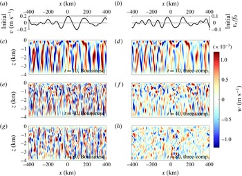
The vertical velocities in the Boussinesq and three-component solutions are compared in figures 3 and 4 for initial NIW magnitudes of
 $U_{0}=0.4$
and
 $0.2~\text{m}~\text{s}^{-1}$
. Vertical velocity is plotted from (c,d) to (g,h) at
 $t=10$
, 40 and 80 inertial periods. For both cases, the agreement is good at
 $t=10$
inertial periods but degrades progressively thereafter. Conspicuous aspects of the Boussinesq solution absent from the three-component solution are features with small horizontal scales and steep characteristic angles. These features are especially prominent in figure 3 for the most nonlinear case with
 $U_{0}=0.4~\text{m}~\text{s}^{-1}$
at
 $t=40$
and 80 inertial periods.
Comparison of the vertical velocity in numerical solutions with the Boussinesq and three-component models. (a,b) The
 $x$
dependence of the initial
 $v$
(a) and
 $v_{x}/f_{0}$
(b). (c–h) The vertical velocity
 $w$
at
 $t=10$
, 40 and 80 inertial periods for the Boussinesq model (c,e,g) and the three-component model (d,f,h). The initial NIW surface velocity is
 $U_{0}=0.4~\text{m}~\text{s}^{-1}$
.

Like figure 3 but with initial NIW surface velocity
 $U_{0}=0.2~\text{m}~\text{s}^{-1}$
. The agreement between the Boussinesq and three-component models is better than for
 $U_{0}=0.4~\text{m}~\text{s}^{-1}$
.

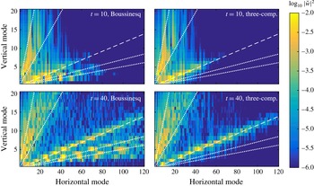
We dissect this failure of the three-component model in figure 5, which compares vertical kinetic energy (VKE) spectra between the three-component and Boussinesq models for
 $U_{0}=0.4~\text{m}~\text{s}^{-1}$
at
 $t=10$
and 40 inertial periods. The five lines indicate internal wave frequencies based on the linear dispersion relation; proceeding clockwise from the vertical axes these frequencies are
 $1.01f_{0}$
,
 $1.08f_{0}$
,
 $2f_{0}$
,
 $3f_{0}$
and
 $4f_{0}$
, with the dashed line corresponding to
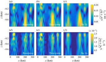
 $2f_{0}$
. The dynamics are clear: in the Boussinesq simulations, substantial VKE leaks into higher harmonic frequencies
 $3f_{0}$
and
 $4f_{0}$
. By
 $t=40$
inertial periods, the fraction of VKE contained in frequencies greater than
 $2.8f_{0}$
is 49 %. This transfer of VKE to higher harmonics decreases with
 $U_{0}$
: for
 $U_{0}=0.2$
and
 $0.1~\text{m}~\text{s}^{-1}$
, the fraction is 10 % and just over 1 % respectively at
 $t=40$
inertial periods.
Snapshots of VKE spectral components,
 $|\breve{w}|^{2}$
, where
 $\breve{w}$
denotes the Fourier and vertical mode transform of
 $w$
, for
 $U_{0}=0.4~\text{m}~\text{s}^{-1}$
at
 $t=10$
and 40 inertial periods. The spectral components are normalized by the total Boussinesq VKE, and horizontal modes include energy from both positive and negative horizontal wavenumbers. The five lines show the linear dispersion relation for five internal wave frequencies; proceeding clockwise from the vertical axes these frequencies are
 $1.01f_{0}$
,
 $1.08f_{0}$
,
 $2f_{0}$
,
 $3f_{0}$
and
 $4f_{0}$
, with the dashed line corresponding to
 $2f_{0}$
. By
 $t=40$
inertial periods, 49 % of the Boussinesq VKE is in frequencies higher than
 $2.8f_{0}$
.

The effect of the energy transfer to NIW harmonics on total VKE is demonstrated in figure 6, which shows the evolution of total VKE,
 $\int w^{2}/2\,\text{d}x\,\text{d}z$
, for (a)
 $U_{0}=0.4~\text{m}~\text{s}^{-1}$
and (b)
 $U_{0}=0.2~\text{m}~\text{s}^{-1}$
. Four models are considered: Boussinesq (solid lines), three-component model (dashed lines), a two-component model that neglects
 $2f_{0}$
(dash-dotted lines), and a modification of the three-component model with PSI suppressed by removing
 $B_{xx}\text{L}\,A^{\ast }$
from the NIW equation (7.4) (dotted line, figure 6(b) only). The three-component model underestimates the amplitude of the VKE, having 54 % of the Boussinesq solution at
 $t=40$
inertial periods and 43 % of the total at
 $t=80$
inertial periods. The ‘extra’ Boussinesq VKE is thus similar to that contained in frequencies greater than
 $2.8f_{0}$
, implying that it originates in a transfer of horizontal NIW kinetic energy to high NIW harmonics not accounted for in the three-component model. It is not surprising that this transfer to
 $3f_{0}$
and
 $4f_{0}$
is strongest in the most nonlinear case with
 $U_{0}=0.4~\text{m}~\text{s}^{-1}$
.
Evolution of total VKE,
 $\int w^{2}/2\,\text{d}x\,\text{d}z$
, for (a)
 $U_{0}=0.4~\text{m}~\text{s}^{-1}$
and (b)
 $U_{0}=0.2~\text{m}~\text{s}^{-1}$
. Results are diagnosed from the Boussinesq model (solid lines), the three-component model (dashed lines), a ‘no
 $2f_{0}$
’ two-component model with
 $B\mapsto 0$
(dash-dotted lines) and a ‘no PSI’ three-component model with the term
 $B_{xx}\text{L}\,A^{\ast }$
removed from the NIW equation (7.4) (dotted line in (b) only). Black colours are used for (a)
 $U_{0}=0.4~\text{m}~\text{s}^{-1}$
and blue colours for (b)
 $U_{0}=0.2~\text{m}~\text{s}^{-1}$
here and in figures 7 and 9.


Comparison of velocity magnitude and shear magnitude between the Boussinesq equations, the three-component model and a two-component model with
 $B\mapsto 0$
and thus no
 $2f_{0}$
waves. The snapshots are taken at
 $t=80$
inertial periods and comprise a portion of the full domain shown in figure 2.

For the case
 $U_{0}=0.2~\text{m}~\text{s}^{-1}$
the three-component model correctly estimates the amplitude, but not the phase of the VKE. Unsurprisingly, given the impact of NIW–harmonic interactions on the VKE, the two-component solutions with
 $B\mapsto 0$
and thus no
 $2f_{0}$
cannot capture the evolution of the VKE for either
 $U_{0}=0.4$
or
 $0.2~\text{m}~\text{s}^{-1}$
. In figure 6(b), the suppression of PSI leads to an unrealistic accumulation of VKE in
 $2f_{0}$
motions starting at approximately
 $t=20$
inertial periods. This indicates that the transfer of energy from
 $2f_{0}$
back to NIWs must be accounted for to accurately capture VKE evolution.
7.4 Summary
The comparison presented in this section shows that the three-component model well describes NIW evolution and nonlinear NIW–
 $2f_{0}$
interaction. That the three-component model describes NIW evolution in the cases shown here is not too surprising, since it is probably driven by a linearized YBJ-type flow-induced refraction. The success of the three-component model in describing NIW–
 $2f_{0}$
interaction is more surprising and vindicates the heuristic derivation of
 $2f_{0}$
dynamics. On the other hand, the model grossly underestimates the vertical velocity magnitude when the NIWs are strong, which follows from the neglect of NIW harmonics higher than
 $2f_{0}$
. We stress that this two-dimensional comparison cannot test whether the three-component model correctly captures the impact of NIWs on balanced flow evolution.
8 Energy transfer and production of small vertical scales
In this section we continue to explore the initial value problem of § 7 by looking at the energy transfer between the three flow components and the surprising role played by
 $2f_{0}$
in the evolution of the smallest vertical scales.
8.1 Energy transfer between flow components
The two conserved quantities in the three-component model are wave action and coupled energy defined in (6.1) and (6.9) and plotted in figure 7(a,b). Figure 7(a) illustrates the transfer between NIW kinetic energy and the total energy of the
 $2f_{0}$
field, defined respectively as
 $$\begin{eqnarray}\mathscr{A}_{f}=\int \frac{1}{2}|\text{L}\,A|^{2}\,\text{d}x\,\text{d}z\quad \text{and}\quad \mathscr{A}_{2f}=\int {\displaystyle \frac{1}{6}}|B_{x}|^{2}+{\displaystyle \frac{13f_{0}^{2}}{6N^{2}}}|B_{z}|^{2}\,\text{d}x\,\text{d}z.\end{eqnarray}$$
Figure 7(a) shows the components of wave action change
 $\unicode[STIX]{x1D6FF}\mathscr{A}_{f}(t)\stackrel{\text{def}}{=}\mathscr{A}_{f}(t)-\mathscr{A}(0)$
and
 $\mathscr{A}_{2f}$
. Figure 7(a) also shows the very small change in total wave action
 $\unicode[STIX]{x1D6FF}\mathscr{A}=\unicode[STIX]{x1D6FF}\mathscr{A}_{f}+\mathscr{A}_{2f}$
due to hyper-dissipation with dotted lines. All curves are normalized by the initial wave action
 $\mathscr{A}(0)$
, which is equal to the kinetic energy in the near-inertial initial condition. Three cases corresponding to different initial amplitudes of the NIW are shown:
 $U_{0}=0.1,0.2$
and
 $0.4~\text{m}~\text{s}^{-1}$
in red, blue and black. The action transferred from
 $\mathscr{A}_{f}$
to
 $\mathscr{A}_{2f}$
increases initially to a maximum value and thereafter decays to a constant asymptotic value as
 $t\rightarrow \infty$
. Although the short-term maximum transfer increases with the initial NIW amplitude
 $U_{0}$
, the fraction as
 $t\rightarrow \infty$
is independent of
 $U_{0}$
and indicates that less than 1 % of the near-inertial action is ultimately transferred to the
 $2f_{0}$
field.
Figure 7(b) shows the evolution of
 $\unicode[STIX]{x1D6FF}\mathscr{E}_{\unicode[STIX]{x1D713}}(t)\stackrel{\text{def}}{=}\mathscr{E}_{\unicode[STIX]{x1D713}}(t)-\mathscr{E}(0)$
,
 $\mathscr{E}_{f}$
and
 $\mathscr{E}_{2f}$
following the definitions in (6.3), (6.5) and (6.7) respectively. All energies are normalized by the initial near-inertial kinetic energy
 $\mathscr{A}(0)$
, thus revealing an uncanny correspondence between cases: the energy transferred from balanced flow to NIWs is a constant fraction of the initial NIW kinetic energy,
 $\mathscr{A}_{f}(0)$
.
8.2 The
$2f_{0}$
motions are a stepping stone to small vertical scales

The evolution of
 $\mathscr{A}_{2f}$
in figure 7(a) is unspectacular and suggests that NIW–
 $2f_{0}$
interaction is not important because at most a mere 3 % of the initial NIW kinetic energy is transferred to
 $2f_{0}$
when
 $U_{0}=0.4~\text{m}~\text{s}^{-1}$
. Yet the possibility for a PSI-type energy transfer from
 $2f_{0}$
to NIW hints that the inclusion of
 $2f_{0}$
and nonlinear NIW–
 $2f_{0}$
interaction may be necessary to capture the production of small NIW vertical scales.
We isolate the effect of this process by computing a ‘no
 $2f_{0}$
’ solution of (7.3) and (7.4). In this solution we set
 $B\mapsto 0$
, thus removing
 $2f_{0}$
waves and the
 $2f_{0}$
-mediated transfer of energy. Figure 8 gives a qualitative impression of the results, where the wave speed (a–c) and wave shear magnitude (d–f) are plotted for three model solutions with
 $U_{0}=0.4~\text{m}~\text{s}^{-1}$
: Boussinesq (a,d), three-component model (b,e) and the two-component ‘no
 $2f_{0}$
’ solution of (7.3) and (7.4) with
 $B\mapsto 0$
(c,f). Both the Boussinesq and the three-component results have small scales in the vertical velocity which are lacking when
 $2f_{0}$
is removed, and thus must be created by nonlinear NIW–
 $2f_{0}$
interaction. Without
 $2f_{0}$
the magnitude of the vertical shear is also underestimated near
 $(x,z)=(-0.1,40)~\text{km}$
. At the same time, the overall flow structure agrees between the three models.
A more quantitative estimate of small vertical scales is provided by the metric
 $\mathit{Ri}^{\dagger }(t)$
, which measures the smallest Richardson numbers and thus the potential for wave breaking and mixing were such processes resolved. Here,
 $\mathit{Ri}^{\dagger }$
is defined as the average of the smallest 0.1 % of Richardson numbers:
 $$\begin{eqnarray}\mathit{Ri}^{\dagger }(t)\stackrel{\text{def}}{=}\text{mean }[\text{smallest 0.1 }\%\text{ of }\mathit{Ri}\text{ values}],\quad \text{where}\quad \mathit{Ri}\stackrel{\text{def}}{=}\frac{N^{2}+b_{z}}{u_{z}^{2}+v_{z}^{2}}.\end{eqnarray}$$
The evolution of
 $\mathit{Ri}^{\dagger }$
normalized by its initial value is shown in figure 9 for the cases
 $U_{0}=0.4$
and
 $0.2~\text{m}~\text{s}^{-1}$
. Results are compared between the Boussinesq, three-component and two-component models. The comparison reveals that small values of
 $\mathit{Ri}^{\dagger }$
and thus small vertical scales are produced by at least two distinct physical mechanisms:
 $\mathit{Ri}^{\dagger }$
first decreases to a minimum value between
 $t=15$
and 20 inertial periods and rises gradually thereafter. The early-time agreement between all five cases means that
 $\mathit{Ri}^{\dagger }$
is controlled by refraction of the NIW field by balanced flow during this first stage.
The evolution of
 $\mathit{Ri}^{\dagger }$
defined in (8.2) and normalized by its initial value for the cases
 $U_{0}=0.4~\text{m}~\text{s}^{-1}$
(black) and
 $U_{0}=0.2~\text{m}~\text{s}^{-1}$
(blue or grey) and in three models: Boussinesq (solid lines), three-component model (dashed lines) and the two-component model with
 $B\mapsto 0$
and thus no
 $2f_{0}$
(dashed-dotted lines). The inset shows the numerical values of
 $\mathit{Ri}^{\dagger }$
approaching the critical value
 $\mathit{Ri}=1/4$
for the case
 $U_{0}=0.4~\text{m}~\text{s}^{-1}$
in the Boussinesq and three-component models. The metric
 $\mathit{Ri}^{\dagger }$
is a measure of the smallest vertical scales in the flow, whose evolution cannot be captured without
 $2f_{0}$
.

However, at approximately
 $t=40$
inertial periods, the results diverge and
 $\mathit{Ri}^{\dagger }$
is smaller for
 $U_{0}=0.4~\text{m}~\text{s}^{-1}$
in both the Boussinesq and the three-component model. It is conspicuous that in the two-component model with
 $U_{0}=0.4~\text{m}~\text{s}^{-1}$
,
 $\mathit{Ri}^{\dagger }$
is overestimated and stays close to the more linear
 $U_{0}=0.2~\text{m}~\text{s}^{-1}$
results. At this stage, the smallness of
 $\mathit{Ri}^{\dagger }$
and thus small NIW vertical scales in the Boussinesq and three-component models must be controlled by nonlinear NIW–
 $2f_{0}$
interaction. Strikingly, and despite the fact that they contain little instantaneous energy,
 $2f_{0}$
motions provide a crucial stepping stone through which NIW energy is transferred to small vertical scales. The surprisingly accurate description of this process by the three-component model suggests that it is controlled by the interaction of relatively large-vertical-scale
 $2f_{0}$
motions with small-scale NIWs, which figures 2 and 3 show to be well captured by the three-component model.
9 Discussion
We have developed a three-component model for the coupled evolution of NIWs, QG flow and internal waves with frequency near
 $2f_{0}$
. The three-component model adds
 $2f_{0}$
dynamics to the two-component NIW–QG model derived by Xie & Vanneste (Reference Xie and Vanneste2015), and thereby describes the prominent
 $2f_{0}$
vertical velocities and production of small NIW vertical scales that numerical solutions of the Boussinesq equations show to be important features of the coupled evolution of NIWs and balanced flow.
A striking prediction of both the three-component model and XV’s two-component model is that forced oceanic NIWs extract energy from large-scale balanced flows. Because this requires externally forced internal waves, XV call this mechanism ‘stimulated loss of balance’, distinguishing it from the spontaneous loss of balance that occurs without external forcing of waves. Stimulated loss of balance acts even in small-Rossby-number flows, and our numerical solutions suggest that energy transfer to NIWs increases with the strength of the externally forced waves. Gertz & Straub (Reference Gertz and Straub2009) showed that stimulated loss of balance can result in a forward energy cascade and dissipation of wind-driven gyres in an unstratified thin-aspect-ratio fluid. The significance of stimulated loss of balance in real ocean flows is uncertain.
The three-component model connects the
 $2f_{0}$
generation mechanism identified by Danioux & Klein (Reference Danioux and Klein2008) with the YBJ-based near-inertial PSI mechanism of Young et al. (Reference Young, Tsang and Balmforth2008). The form of the NIW–
 $2f_{0}$
coupling implies a two-step cycle for NIW energy. First, advection and refraction by balanced flow catalyses transfer of NIW energy to
 $2f_{0}$
waves. These newly produced
 $2f_{0}$
waves have large, often depth-spanning, vertical scales and propagate rapidly in the horizontal. Second, a PSI-like interaction transfers energy from
 $2f_{0}$
waves back to the NIW field at very small vertical scales. This two-step process provides a path from the large scales of NIW forcing to the small scales of wave breaking and mixing. Advection and refraction of NIWs by non-uniform QG flows leads to relatively small NIW horizontal scales and thus plays a catalytic role in activating this path. Interestingly, the rapid horizontal and vertical propagation of the nascent
 $2f_{0}$
waves can excite small-scale NIWs in regions remote from the initial NIW forcing. Two-dimensional numerical solutions of both the three-component and Boussinesq models give tentative confirmation of this mechanism.
The numerical comparison with the Boussinesq equations shows that the strengths of the three-component model include its description of NIW refraction by balanced flow, and prediction of both the phase and the amplitude of growing
 $2f_{0}$
waves at short times. A weakness of the three-component model is the underestimation of the vertical velocity and vertical kinetic energy under increasingly nonlinear conditions due to its neglect of
 $3f_{0}$
and
 $4f_{0}$
frequency NIW harmonics. Despite this shortcoming, the three-component model captures with surprising accuracy the long-time evolution of the very smallest NIW vertical scales that result from nonlinear NIW–
 $2f_{0}$
interaction.
The numerical comparison primarily tests the accuracy of NIW–
 $2f_{0}$
dynamics in the three-component model in a regime where refraction by APV-induced balanced flow controls the large-scale NIW evolution. The magnitude of APV and the APV-induced flow mean that our comparison does not isolate the existence and impact of balanced flow induced by quadratic NIW terms in (1.7). In addition, because APV cannot evolve from its initial condition in our two-dimensional scenario, the comparison cannot explore dynamic NIW–QG interaction. A three-dimensional comparison of three-component and Boussinesq dynamics is required to define the regimes of validity of the three-component model in more realistic scenarios and to unravel the effects of NIWs and their wave-induced balanced flow on the evolution of oceanic QG motion.
The applicability of the three-component model to a particular part of the ocean can be assessed using kinetic energy frequency spectra derived from long-term mooring observations of horizontal velocity. Where non-wave flows of NIW scale have small Rossby number, the three-component model well approximates the dynamics of any motion with Eulerian frequencies near
 $f_{0}$
. In flows with relative vorticities near or greater than
 $f_{0}$
, or under conditions of active wave breaking, the relevance of the three-component model is uncertain. The ubiquitous appearance of a spectral peak at
 $f_{0}$
combined with the belief that large NIW-scale vortical flows are predominantly balanced (Ferrari & Wunsch Reference Ferrari and Wunsch2009) hints at, but does not confirm, the potentially broad applicability of the three-component model. Such confirmation requires further observations, such as the difficult simultaneous observation of large-scale balanced vorticity and storm-driven NIW evolution. The applicability of the three-component model to real flows is of consequence because prediction of the climatic evolution of diapycnal mixing likely requires a firm understanding of NIW physics – a link between the large and small scales of oceanic motion.
Acknowledgements
This work was supported by the National Science Foundation under OCE-1357047. We thank three anonymous reviewers for their criticism and C. Rocha, N. Grisouard, K. Winters, O. Bühler, J. Vanneste and J.-H. Xie for helpful discussions. N. Grisouard provided source code and selfless assistance in setting up his customized version of Winters’ flowsolve code.
Appendix A. The
$2f_{0}$
equation

In this appendix, we outline the asymptotic and heuristic steps that lead to the
 $2f_{0}$
equation in (1.9) and (5.3).
A.1 The
$2f_{0}$
frequency forcing at first order

The vertically averaged time-fluctuating part of the first-order Boussinesq system in (3.24)–(3.27) is
 $$\begin{eqnarray}\displaystyle & \displaystyle \widehat{\tilde{{\mathcal{U}}}_{1}}_{\,\tilde{t}\,}+\text{i}f_{0}\,\widehat{\tilde{{\mathcal{U}}}_{1}}+2\tilde{p}_{0s^{\ast }}=-\text{e}^{-2\text{i}f_{0}\,\tilde{t}\,}\widehat{{\mathcal{J}}}_{2}, & \displaystyle\end{eqnarray}$$
 $$\begin{eqnarray}\displaystyle & \displaystyle \tilde{p}_{0\bar{z}\,\tilde{t}\,}+\widehat{\tilde{w}_{0}}\,N^{2}=0, & \displaystyle\end{eqnarray}$$
 $$\begin{eqnarray}\displaystyle & \displaystyle \widehat{\tilde{{\mathcal{U}}}_{1}}_{s}+\widehat{\tilde{{\mathcal{U}}}_{1}^{\ast }}_{s^{\ast }}+\widehat{\tilde{w}_{0}}_{\bar{z}}=0, & \displaystyle\end{eqnarray}$$
where the wavy part of the leading-order pressure
 $\tilde{p}_{0}$
does not depend on the fast scale
 $\tilde{z}$
. The system above describes hydrostatic internal waves of general aspect ratio driven by the
 $2f_{0}$
forcing on the right of (A 1).
A bit of wrangling with (A 1)–(A 3) leads to a single equation for the wavy part of the leading-order pressure field:
 $$\begin{eqnarray}\unicode[STIX]{x2202}_{\,\tilde{t}\,}[\,\unicode[STIX]{x2202}_{\,\tilde{t}\,}^{2}\,\bar{\text{L}}+f_{0}^{2}(\unicode[STIX]{x0394}+\bar{\text{L}})]\tilde{p}_{0}=3\text{i}f_{0}^{3}(\text{e}^{-2\text{i}f_{0}\,\tilde{t}\,}\widehat{{\mathcal{J}}}_{2s}-\text{e}^{2\text{i}f_{0}\,\tilde{t}\,}\widehat{{\mathcal{J}}}_{2s^{\ast }}^{\ast }).\end{eqnarray}$$
Equation (A 4) is the hydrostatic internal wave equation forced at frequency
 $2f_{0}$
. Writing
 $\tilde{p}_{0}$
as
 $$\begin{eqnarray}\tilde{p}_{0}=\text{i}f_{0}[\text{e}^{-2\text{i}f_{0}\,\tilde{t}\,}B(x,y,\bar{z},\bar{t})-\text{e}^{2\text{i}f_{0}\,\tilde{t}\,}B^{\ast }(x,y,\bar{z},\bar{t})],\end{eqnarray}$$
and noting that (3.16a,b ) implies
 $$\begin{eqnarray}\widehat{{\mathcal{J}}}_{2}=\unicode[STIX]{x2202}_{s}\,\widehat{M_{\tilde{z}}^{2}},\end{eqnarray}$$
we find that
 $B$
satisfies
 $$\begin{eqnarray}\text{i}f_{0}(\unicode[STIX]{x0394}-3\bar{\text{L}})B=-{\textstyle \frac{3}{2}}\unicode[STIX]{x2202}_{s}^{2}\,\widehat{M_{\tilde{z}}^{2}}.\end{eqnarray}$$
A.2 Resonant and near-resonant NIW–
$2f_{0}$
interaction

Equation (A 7) describes forced oscillations with frequency
 $2f_{0}$
. It cannot describe the resonant and near-resonant generation and free propagation of
 $2f_{0}$
internal waves. Near-resonant generation can be understood by projecting (A 7) onto vertical modes
 $\mathit{h}_{n}(z)$
which satisfy
 $$\begin{eqnarray}\text{L}\mathit{h}_{n}+\unicode[STIX]{x1D705}_{n}^{2}\mathit{h}_{n}=0\quad \text{and}\quad \mathit{h}_{n}^{\prime }=0\quad \text{at top and bottom,}\end{eqnarray}$$
where the eigenvalue
 $\unicode[STIX]{x1D705}_{n}$
is the Rossby deformation wavenumber of mode
 $n$
. If we look for solutions of the form
 $B\sim \text{e}^{\text{i}kx+\text{i}\ell y}h_{n}(z)$
, we find that (A 7) cannot be solved when
 $$\begin{eqnarray}k^{2}+\ell ^{2}=3\unicode[STIX]{x1D705}_{n}^{2}.\end{eqnarray}$$
These combinations, which are circular slices of
 $(k,\ell )$
space at each vertical mode, are the wavenumber combinations that satisfy the linear internal wave dispersion relation at frequency
 $2f_{0}$
. Freely propagating
 $2f_{0}$
internal waves are generated when the NIW forcing
 $\unicode[STIX]{x2202}_{s}^{2}\widehat{M}_{\tilde{z}}^{2}$
has non-zero spectral content near these wavenumber combinations. The generality of near-resonant
 $2f_{0}$
generation in NIW–balanced-flow interaction is evident from the results in figure 1 and the simulations in Danioux et al. (Reference Danioux, Klein and Rivière2008).
As resonant generation is generic, we seek to describe it by modifying (A 7). In particular, we need a term proportional to
 $B_{\bar{t}}$
in (A 7) in order to describe time-dependent
 $B$
generation and free near-
 $2f_{0}$
propagation. We achieve this by applying the map
 $$\begin{eqnarray}\unicode[STIX]{x2202}_{t}\mapsto -2\text{i}f_{0}+\unicode[STIX]{x2202}_{\bar{t}}\end{eqnarray}$$
to (A 4) and re-deriving the
 $2f_{0}$
equation.
The scaling in § 2.1 implies that
 $\unicode[STIX]{x2202}_{\bar{t}}$
is
 $\unicode[STIX]{x1D716}^{2}$
smaller than
 $2f_{0}$
; thus, in applying (A 10) to (A 4) we ignore the even smaller
 $O(\unicode[STIX]{x1D716}^{4})$
terms. Introducing (A 5) into the result then yields
 $$\begin{eqnarray}-(\unicode[STIX]{x0394}-11\bar{\text{L}})B_{\bar{t}}+2\text{i}f_{0}(\unicode[STIX]{x0394}-3\bar{\text{L}})B=-3\unicode[STIX]{x2202}_{s}^{2}\widehat{M_{z}^{2}}.\end{eqnarray}$$
The leftmost term is
 $\unicode[STIX]{x1D716}^{2}$
smaller than
 $(\unicode[STIX]{x0394}-3\bar{\text{L}})B$
and only becomes important when
 $(\unicode[STIX]{x0394}-3\bar{\text{L}})B\approx 0$
. Moreover, the addition of any multiple of
 $(\unicode[STIX]{x0394}-3\bar{\text{L}})B_{\bar{t}}$
does not reduce the ‘accuracy’ of the approximation in (A 11).
We exploit this ambiguity to improve the already approximate form of (A 11). Consider the exact vertical mode-
 $n$
dispersion relation for linear hydrostatic internal waves,
 $$\begin{eqnarray}\unicode[STIX]{x1D6F4}=\pm f_{0}\sqrt{1+\frac{k^{2}}{\unicode[STIX]{x1D705}_{n}^{2}}},\end{eqnarray}$$
where
 $\unicode[STIX]{x1D6F4}(k,\unicode[STIX]{x1D705}_{n})$
is the hydrostatic internal wave frequency,
 $k$
is the horizontal wavenumber and
 $\unicode[STIX]{x1D705}_{n}$
is the horizontal wavenumber of the
 $n\text{th}$
vertical mode. The Taylor expansion of the positive root of
 $\unicode[STIX]{x1D6F4}$
around
 $k=\sqrt{3}\unicode[STIX]{x1D705}_{n}$
with
 $\unicode[STIX]{x1D705}_{n}$
fixed is
 $$\begin{eqnarray}\unicode[STIX]{x1D6F4}=2f_{0}+\frac{\sqrt{3}f_{0}}{2\unicode[STIX]{x1D705}_{n}}(k-\sqrt{3}\unicode[STIX]{x1D705}_{n})+\frac{f_{0}}{16\unicode[STIX]{x1D705}_{n}^{2}}(k-\sqrt{3}\unicode[STIX]{x1D705}_{n})^{2}+\cdots .\end{eqnarray}$$
On the other hand, the approximate dispersion relation implied by (A 11) is found by linearizing (A 11), projecting it onto vertical modes and proposing
 $B\sim \text{e}^{\text{i}kx-\text{i}\unicode[STIX]{x1D70E}\bar{t}}$
so that the frequency of
 $B$
is
 $2f_{0}+\unicode[STIX]{x1D70E}$
. Algebra reveals that
 $\unicode[STIX]{x1D6F4}_{k}=\unicode[STIX]{x1D70E}_{k}$
when
 $k=\sqrt{3}\unicode[STIX]{x1D705}_{n}$
and
 $\unicode[STIX]{x1D6F4}=2f_{0}$
. As a consequence, the
 $2f_{0}$
approximation in (A 11) produces the correct group velocity.
This feature is preserved under the addition of any multiple of
 $(\unicode[STIX]{x0394}-3\bar{\text{L}})B_{\bar{t}}$
to (A 11). We use this freedom to increase the accuracy of
 $2f_{0}$
linear dispersion in the three-component model. Subtracting
 $(9/2)(\unicode[STIX]{x0394}-3\bar{\text{L}})B_{\bar{t}}$
from (A 11), we obtain
 $$\begin{eqnarray}(\unicode[STIX]{x0394}+13\bar{\text{L}})B_{\bar{t}}+4\text{i}f_{0}(\unicode[STIX]{x0394}-3\bar{\text{L}})B=-6\unicode[STIX]{x2202}_{s}^{2}\widehat{M_{\tilde{z}}^{2}}.\end{eqnarray}$$
The approximate dispersion relation implied by (A 14) is
 $$\begin{eqnarray}\unicode[STIX]{x1D70E}=4f_{0}\frac{k^{2}-3\unicode[STIX]{x1D705}_{n}^{2}}{k^{2}+13\unicode[STIX]{x1D705}_{n}^{2}},\end{eqnarray}$$
which yields
 $\unicode[STIX]{x1D70E}_{kk}=\unicode[STIX]{x1D6F4}_{kk}$
and means that (A 14) produces the correct near-
 $2f_{0}$
group velocity over a range of wavenumbers. Figure 10 compares the exact dispersion relation with the approximate dispersion relations for both the
 $2f_{0}$
harmonic component as well as the NIW component, demonstrating the accuracy of our ‘Padé’ approximation to the
 $2f_{0}$
dispersion relation. We use (A 14) to model the
 $2f_{0}$
component of flow in the three-component system. It should be noted also that such a ‘Padé’ approximation can be applied in the same manner to the NIW equation.
Comparison between the exact hydrostatic internal wave dispersion relation and the approximate linear dispersion relations in the three-component model. The thick black line traces the exact hydrostatic internal wave dispersion relation. The green dash-dotted line is the approximate dispersion relation for the NIW component,
 $f_{0}(1+k^{2}/2\unicode[STIX]{x1D705}_{n}^{2})$
, obtained by linearizing (1.8). The blue dashed line is the approximate dispersion relation for the
 $2f_{0}$
component implied by (1.9) and (A 14) and given by
 $2f_{0}+\unicode[STIX]{x1D70E}$
in (A 15). The insets show the fractional errors of the approximate NIW and
 $2f_{0}$
dispersion relations.

A.3 Expressions for
${\mathcal{U}}_{1}$
and
${\hat{w}}_{0}$


With
 $\tilde{p}_{0}$
defined through
 $B$
, we can calculate
 $\tilde{{\mathcal{U}}}_{1}$
. The vertically averaged horizontal momentum equation is
 $$\begin{eqnarray}\displaystyle \widehat{\tilde{{\mathcal{U}}}}_{1\,\tilde{t}\,}+\text{i}f_{0}\widehat{\tilde{{\mathcal{U}}}}_{1} & = & \displaystyle -2\tilde{p}_{0s^{\ast }}-\text{e}^{-2\text{i}f_{0}\,\tilde{t}\,}\widehat{{\mathcal{J}}}_{2},\end{eqnarray}$$
 $$\begin{eqnarray}\displaystyle & = & \displaystyle -2\text{i}f_{0}\text{e}^{-2\text{i}f_{0}\,\tilde{t}\,}B_{s^{\ast }}+2\text{i}f_{0}\text{e}^{2\text{i}f_{0}\,\tilde{t}\,}B_{s^{\ast }}^{\ast }-\text{e}^{-2\text{i}f_{0}\,\tilde{t}\,}\unicode[STIX]{x2202}_{s}\widehat{M}_{z}^{2},\end{eqnarray}$$
which means that
 $$\begin{eqnarray}\widehat{\tilde{{\mathcal{U}}}}_{1}=\text{e}^{-2\text{i}f_{0}\,\tilde{t}\,}(2B_{s^{\ast }}-\text{i}f_{0}^{-1}\unicode[STIX]{x2202}_{s}\widehat{M}_{z}^{2})+{\textstyle \frac{2}{3}}\text{e}^{2\text{i}f_{0}\,\tilde{t}\,}B_{s^{\ast }}^{\ast }.\end{eqnarray}$$
The vertically averaged vertical velocity
 ${\hat{w}}_{0}$
is obtained from (A 2),
 $$\begin{eqnarray}{\hat{w}}_{0}=-\frac{2f_{0}^{2}}{N^{2}}(\text{e}^{-2\text{i}f_{0}\,\tilde{t}\,}B_{\bar{z}}+\text{e}^{2\text{i}f_{0}\,\tilde{t}\,}B_{\bar{z}}^{\ast }).\end{eqnarray}$$
With
 ${\hat{w}}_{0}$
we can obtain the full expression for
 $\tilde{{\mathcal{U}}}_{1}$
by solving (3.24), which yields
 $$\begin{eqnarray}\tilde{{\mathcal{U}}}_{1}=\text{e}^{-2\text{i}f_{0}\,\tilde{t}\,}(2B_{s^{\ast }}-\text{i}f_{0}^{-1}{\mathcal{J}}_{2})+{\displaystyle \frac{2}{3}}\text{e}^{2\text{i}f_{0}\,\tilde{t}\,}B_{s^{\ast }}^{\ast }+\frac{f_{0}}{N^{2}}M_{\tilde{z}\tilde{z}}(\text{e}^{-3\text{i}f_{0}\,\tilde{t}\,}B_{\bar{z}}-\text{e}^{\text{i}f_{0}\,\tilde{t}\,}B_{\bar{z}}^{\ast }).\end{eqnarray}$$