1 Introduction
One of the key challenges associated with the operation of floating liquefied natural gas (FLNG) production facilities at sea is to offload LNG at regular intervals from the production barge to a carrier. Side-by-side offloading is the most viable method at present; in this case two very large floating vessels must remain in very close proximity due to the limited size of fenders and loading arms currently available. In such a scenario, any large relative motion between the carrier (e.g. bridge wing) and the FLNG risks a steel-on-steel collision. To guarantee the safety of side-by-side offloading, the maximum roll motion of LNG carriers, which in isolation is much larger than that of FLNG facilities (Zhao et al. Reference Zhao, Yang, Hu and Tao2014), has to be limited to some (small) angle. During offloading, when storage tanks are inevitably partially filled, wave-induced motions of the vessels might excite significant liquid cargo sloshing inside the tanks. In return, this nonlinear sloshing flow could back-react on the vessel motion, affecting the roll response and possibly further limiting the operational sea-state window. As a consequence, the roll behaviour of a carrier vessel with partially filled tanks is of considerable practical importance.
Many studies analysing the roll response of ship-like vessels have been conducted. Viscous damping needs to be included in order to match experimental data and full-scale experience (e.g. Bhattacharyya Reference Bhattacharyya1978, van Dijk, Quiniou-Ramus & Le-Marechal Reference van Dijk, Quiniou-Ramus and Le-Marechal2003). Possible sources of roll damping include: skin friction, eddies due to flow separation (sometimes enhanced by the addition of bilge keels), dynamic lift (with forward speed), all in addition to inviscid wave radiation damping (Ikeda, Himeno & Tanaka Reference Ikeda, Himeno and Tanaka1978; Himeno Reference Himeno1981; Downie, Bearman & Graham Reference Downie, Bearman and Graham1988). Of these sources, radiation damping may be predicted reliably through potential flow theory, but the other terms are still a challenge to model. Although damping may be estimated using semi-empirical or empirical methods, the underlying rationale for choosing a damping coefficient varies from practitioner to practitioner (Himeno Reference Himeno1981). To add to the problem, the prediction of roll response becomes even more complex when taking into account coupling effects due to liquid cargo motion.
There have been classical numerical studies on the coupled problem which start by ignoring the nonlinearity of the sloshing flows inside the tanks (Molin et al. Reference Molin, Remy, Rigaud and De Jouette2002; Malenica, Zalar & Chen Reference Malenica, Zalar and Chen2003; Newman Reference Newman2005). However, sloshing inside tanks can be a strongly nonlinear phenomenon. Faltinsen et al. (Reference Faltinsen, Rognebakke, Lukovsky and Timokha2000), Faltinsen, Rognebakke & Timokha (Reference Faltinsen, Rognebakke and Timokha2003) developed a nonlinear multimodal method for sloshing, which has been adopted for tanks with different (vertical walled) shapes. This method was then applied to spherical tanks, using the analytically approximate sloshing modes of Faltinsen & Timokha (Reference Faltinsen and Timokha2012), with the aim of investigating the stability of steady-state sloshing responses (Faltinsen & Timokha Reference Faltinsen and Timokha2013a ,Reference Faltinsen and Timokha b ). To consider nonlinear sloshing flows, Lee & Kim (Reference Lee and Kim2010) conducted simulations in the time domain using a finite difference computational fluid dynamics (CFD) method and linear potential flow for the external waves. Based on a finite element method for the simulation of nonlinear sloshing, Mitra et al. (Reference Mitra, Wang, Reddy and Khoo2012) ran time domain simulations where nonlinear ship motion was assumed. They found it difficult to obtain converged results for the coupled problem based on CFD, and hence needed experiments to validate the numerical simulations. Nam & Kim (Reference Nam and Kim2007) carried out an experimental study on a barge equipped with two partially filled prismatic tanks, showing the importance of a fully coupled analysis, in particular for roll response. Kim (Reference Kim2007) investigated the nonlinear effect of sloshing on roll response from both experiments and numerical simulations, emphasizing its critical role in the coupling effects. With a similar experimental set-up, Nasar, Sannasiraj & Sundar (Reference Nasar, Sannasiraj and Sundar2008, Reference Nasar, Sannasiraj and Sundar2010) conducted a study on the effects of intermediate filling conditions. Focusing on the roll response, Zhao & McPhail (Reference Zhao and McPhail2017) further clarified some of the effects of liquid cargo sloshing inside spherical tanks on global roll responses.
The majority of these numerical and experimental studies directed their efforts toward improving the prediction of the global roll response coupled with liquid cargo motions considering nonlinearity. However, it is unclear how or if the internal sloshing couples to global roll motions and the role of linearity and nonlinearity in the coupling has not yet been identified. It is known that an obvious secondary resonant response peak is sometimes observed for roll response amplitude operators (RAO) of a vessel with partially filled tanks (Nasar et al. Reference Nasar, Sannasiraj and Sundar2010; Zhao et al. Reference Zhao, Yang, Hu and Tao2014). The secondary peak is generally located at a frequency significantly higher than that of the main roll resonant response. This means that, although there might be some linear wave excitation at the lowest sloshing frequency in real sea states, it is also possible that higher (e.g. double and triple frequency) harmonics of the main roll response peak may excite sloshing of the tank contents, and this internal motion could back-react on the vessel’s roll motion. This coupling process has not been investigated in detail due to its complexity.
To obtain physical understanding of the interactions between external waves, roll motions and internal sloshing, a series of experiments was conducted for a single barge-like model with two identical spherical tanks under the excitation of random seas with a broadbanded spectrum. The role of linear and nonlinear coupling between them is identified, and complexity of this coupling driven by a very broadbanded incident wave field is revealed.
A NewWave-type methodology (Tromans, Anaturk & Hagemeijer Reference Tromans, Anaturk and Hagemeijer1991; Jonathan & Taylor Reference Jonathan and Taylor1997) is adopted to examine the nature of the interactions. This paper can be regarded as the third part of our recent NewWave-type analysis. The first paper (Zhao et al.
Reference Zhao, Wolgamot, Taylor and Eatock Taylor2017) used NewWave-type transient wave groups (with four different phases at intervals of
 $90^{\circ }$
) as input to excite the gap resonance between two vessels, making it possible to extract the higher harmonics of the gap resonance. The second part (Zhao et al.
Reference Zhao, Taylor, Wolgamot and Eatock Taylor2018) used the same experimental configuration as in part 1, but the incident waves were changed to random seas with a broadbanded spectrum and thus more difficult to analyse. Through an averaging process, NewWave-type profiles (similar to the four phase signals in part 1) were obtained in part 2, making it possible to demonstrate the linearity and reciprocity of a linear system response under a random excitation. The viscous damping of the gap resonance phenomenon was observed to have a linear form at laboratory scale. The present study extends the NewWave-type analysis methodology in the second paper by introducing a conditioning process, where for the first time it is extended to represent the average properties of roll and sloshing motions. Based on the NewWave-type analysis in this study, the nonlinearities in the roll responses with internal sloshing are identified. To the authors’ knowledge, our observations of the internal sloshing coupled to higher harmonics of the main resonant roll response are new.
The experimental set-up is described in detail in § 2, followed by the presentation of the measured time histories (in § 3). NewWave-type statistical analysis is performed for large roll peak profiles in § 4, to confirm the feasibility of this approach for large roll motion events. The general character of the vessel motions and internal sloshing excited by broadbanded external waves are illustrated in § 5.1, showing complex coupling between them. In § 5.2, the NewWave analysis coupled to the phase-combination method is presented, enabling the extraction of the higher harmonics of the main roll response coupled to the internal sloshing mode. This is a new observation. Finally, the linear and nonlinear coupling between external waves, ship motions and internal fluid sloshing is explored in § 6.
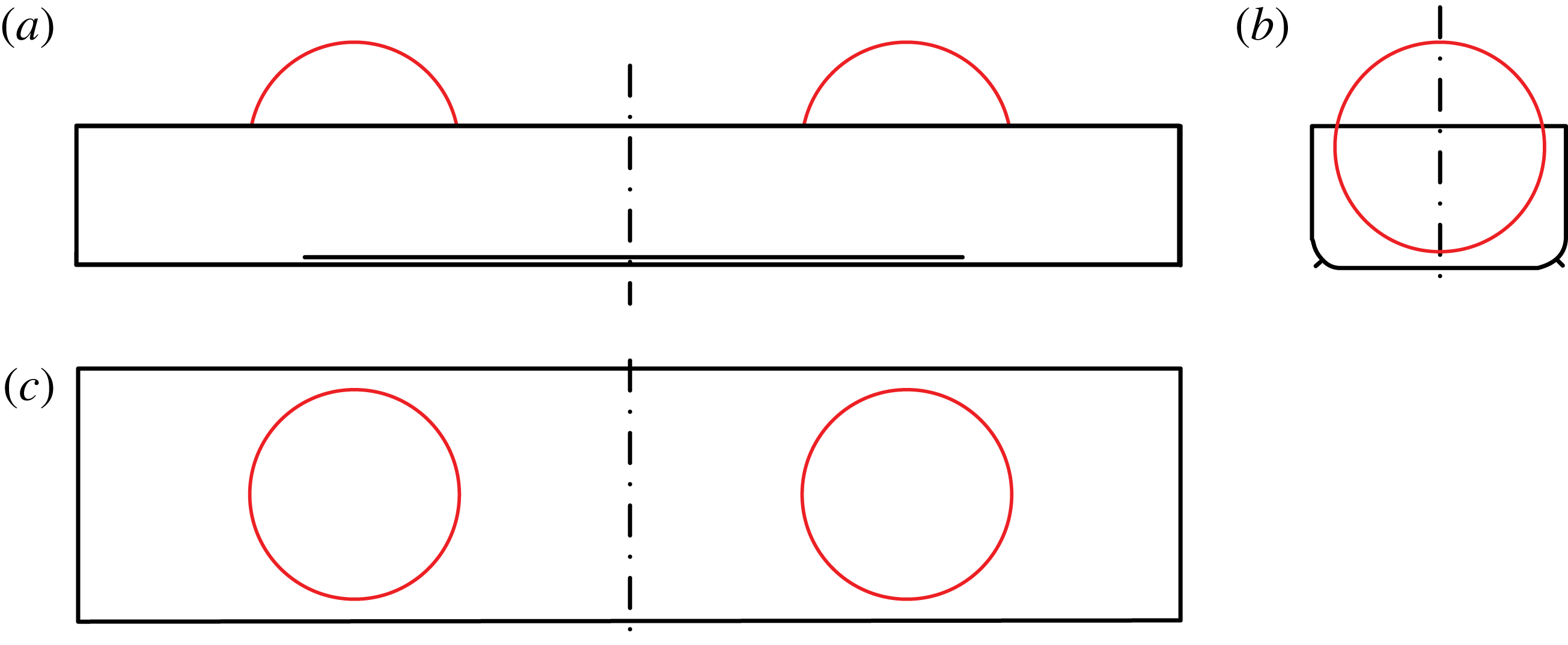
Line drawings of the vessel model with two spherical tanks: (a) broadside view; (b) end-on view; (c) plan view; the radius of the round corners in (b) is 0.083 m; the centre of the spherical tank is 0.833 m from the middle of the model and 0.363 m above the base of the model.

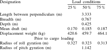
Particulars of the vessel model with two spherical tanks.

2 Experimental set-up
Model tests were conducted in the Deepwater Wave Basin in Shanghai Jiao Tong University. This wave basin is 50 m long, 40 m wide and the water depth was set to 10 m. Waves can be generated by flap-hinged wave makers along one side of the basin and wave absorbers are installed on the opposite side to minimize reflected wave energy from the boundaries of the basin.
2.1 Model details
A barge-like vessel model 3.333 m long and 0.767 m wide (shown in figure 1) was designed to have roll characteristics representative of a Moss-type LNG carrier with spherical storage tanks. The vessel model has rounded corners of radius 0.083 m, and is fitted with bilge keels 0.013 m wide running 2.083 m along the vessel. We are unaware of any liquid that possesses the same density as LNG (
 ${\sim}465~\text{kg}~\text{m}^{-3}$
) and can be used in the laboratory at normal temperature. Hence, to achieve a representative model, two spherical tanks (instead of four in a typical LNG carrier) are installed in the model and filled with fresh water. The internal diameter of these is 0.642 m. Since water is close to twice as dense as LNG, a similar moving mass is present. Since we focus on roll, this model configuration should make the obtained results realistic and valuable for practical assessments, which has not always been possible in previous studies.
Because our focus is on roll coupling to liquid cargo motions, partially filled tanks are required. Tests were conducted with tanks 25 %, 50 % and 75 % full (by volume). The particulars of the vessel in the three different load conditions are listed in table 1. The mean draft does not change significantly as the volume filling level of the spherical tanks is varied. In practice, water inside ballast tanks would be removed during LNG loading, so that the draft of the carrier would hardly change. Also, each ballast tank is required to be either empty or full, to avoid any free-surface effects affecting the global motions of vessel. Hence, for these model tests the ballast tanks are treated as frozen masses, and liquid motion inside the model is only possible within the two partially filled storage tanks.
Based on the above specification, the overall aim of these tests is to provide information relevant to the roll characteristics of a realistic LNG carrier of order 250 m long, 50 m wide and with 4 spherical tanks of diameter 40 m. From the model in the tank to field scale, we have a Froude length scaling of 1 : 60.
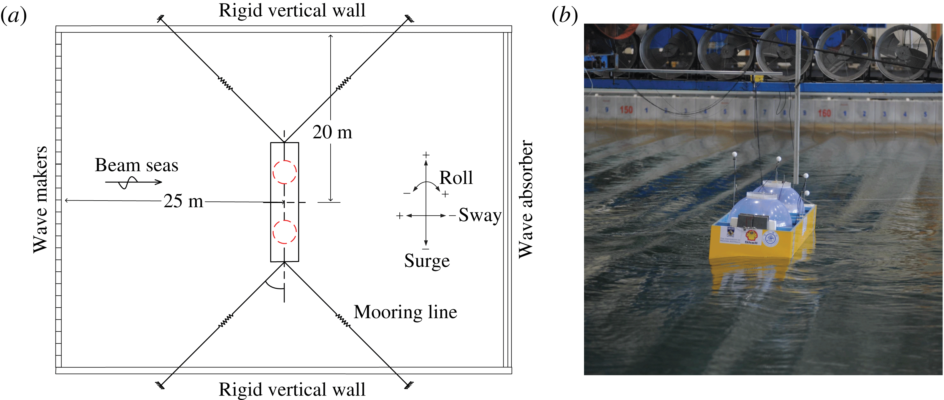
During the experiments, the model was moored in the wave basin with a horizontal mooring system, as shown in figure 2. The horizontal mooring system was designed to prevent the vessel drifting away, but to be soft enough not to introduce any significant restraint at the frequencies of interest. Consequently there is considerable low frequency horizontal motion of the model. The natural period of this induced low frequency motion of the model was measured to be approximately 20 s, which is far beyond any periods of interest here. This study focuses on the roll response in beam seas, as shown in figure 2, which is likely to be the most severe heading condition for the excitation of roll for a moored barge-like vessel. In practice, this could occur in a sea state dominated by swell, but with the vessel direction being controlled by wind and/or tidal currents, or held in position by a dynamic positioning system.
Configuration of the horizontally moored system: (a) schematic of the configuration, (b) the physical model in the wave basin.

2.2 White noise wave generation
Uni-directional waves with a white noise spectrum over a frequency range 0.27–1.94 Hz are used. This spectrum is close to flat and very broad, so it is not fully representative of real ocean wave fields. When Froude scaled to field scale, this wave field would contain wave components of periods 4–29 s. The laboratory-scale significant wave height is 5 cm, so the undisturbed waves remain close to linear and the excited large roll responses are in the desired range of
 ${\sim}3.5^{\circ }$
. The maximum allowable roll response of an LNG carrier during loading is small for side-by-side offloading, so our experiments are directly relevant to this scenario.
The white noise wave field was calibrated prior to the actual model tests, so measured without the model in the wave basin. At laboratory scale each random wave test was run for
 ${\sim}1500$
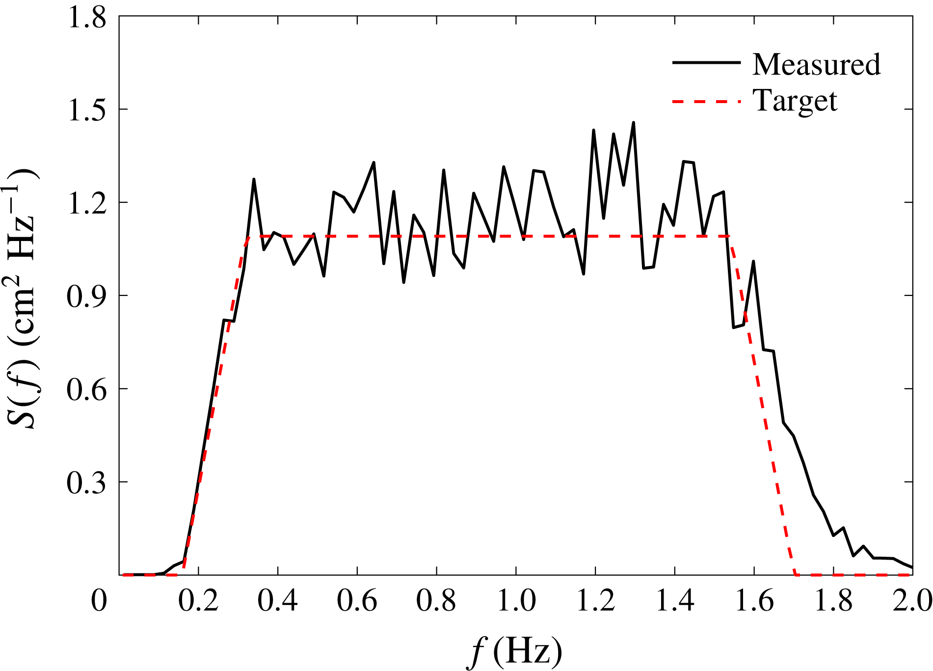
s. The measured spectrum of the broadbanded white noise waves generated in the wave basin for one such test is shown in figure 3. Then, with the model in place, the same paddle signal was used to generate identical incident wave conditions to excite the vessel motions. Note that the agreement (figure 3) between the measured and target spectra at high frequency could be improved with iteration. However, we did not make that effort, as the target spectral shape is essentially arbitrary, provided that it is sufficiently broadbanded to excite both the main roll resonant response and the internal sloshing modes. What is important for our analysis is that the undisturbed waves are known.
The power spectrum (
 $S(f)$
) of surface elevation for the white noise waves generated in the wave basin.

2.3 Mass property adjustment of the model
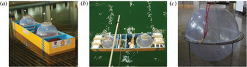
Several tests at the 50 % load condition were performed for which the tanks were empty, but the vessel properties modified to a ‘frozen’ approximation by replacing the liquid with steel weights. Figure 4(a) shows the vessel model with liquid cargo, and (b) ‘frozen’ cargo as weights at each end and in the middle of the model.
The vessel model at the 50 % load condition: (a) liquid cargo (coloured water) in the two spherical tanks, (b) frozen cargo (the white blocks within the model) load condition, (c) curved wave probes inside an empty spherical tank.

Prior to the model tests, the mass properties of the model were adjusted to achieve the target values listed in table 1. This included tuning the location of the centre of gravity, and the mass radii of gyration for the roll and pitch motions. There are two static effects from the liquid free surface inside the tanks; these are the upwards shift of the centre of gravity vertically, and the decrease of the total mass radii of gyration. The former effect was accounted for through the metacentric height correction, while the latter one was accounted for by matching the roll natural period of the model with frozen cargo to that of the liquid cargo case. As a consequence, the only significant difference between the liquid and frozen cargo cases lies in the sloshing of the fluid inside the spherical tanks.
Arc-shaped wave probes were designed and fixed along the curved inner wall of the spherical tanks, as shown in figure 4(c). Before the installation of the barge model, a resistance-type wave probe with measuring error smaller than 1 mm was mounted at the location of the geometric centre of the vessel model (in undisturbed conditions) during the wave calibration process (see § 2.2), and subsequently removed during the model tests. In the model tests, the motions of the model were captured with a Qualisys three-dimensional non-contact optical motion capture system. As can be seen in figure 4, optical balls were fixed to different locations on the model to define rigid body motion. This motion capture system was calibrated immediately after installation, and the desired measurement accuracy was ensured by keeping residual values less than 1 mm.
All the instruments were calibrated prior to the model tests, details of which are given in appendix B. During the model tests, all signals were recorded synchronously at a sampling rate of 25 Hz.
3 Time histories of the measured signals
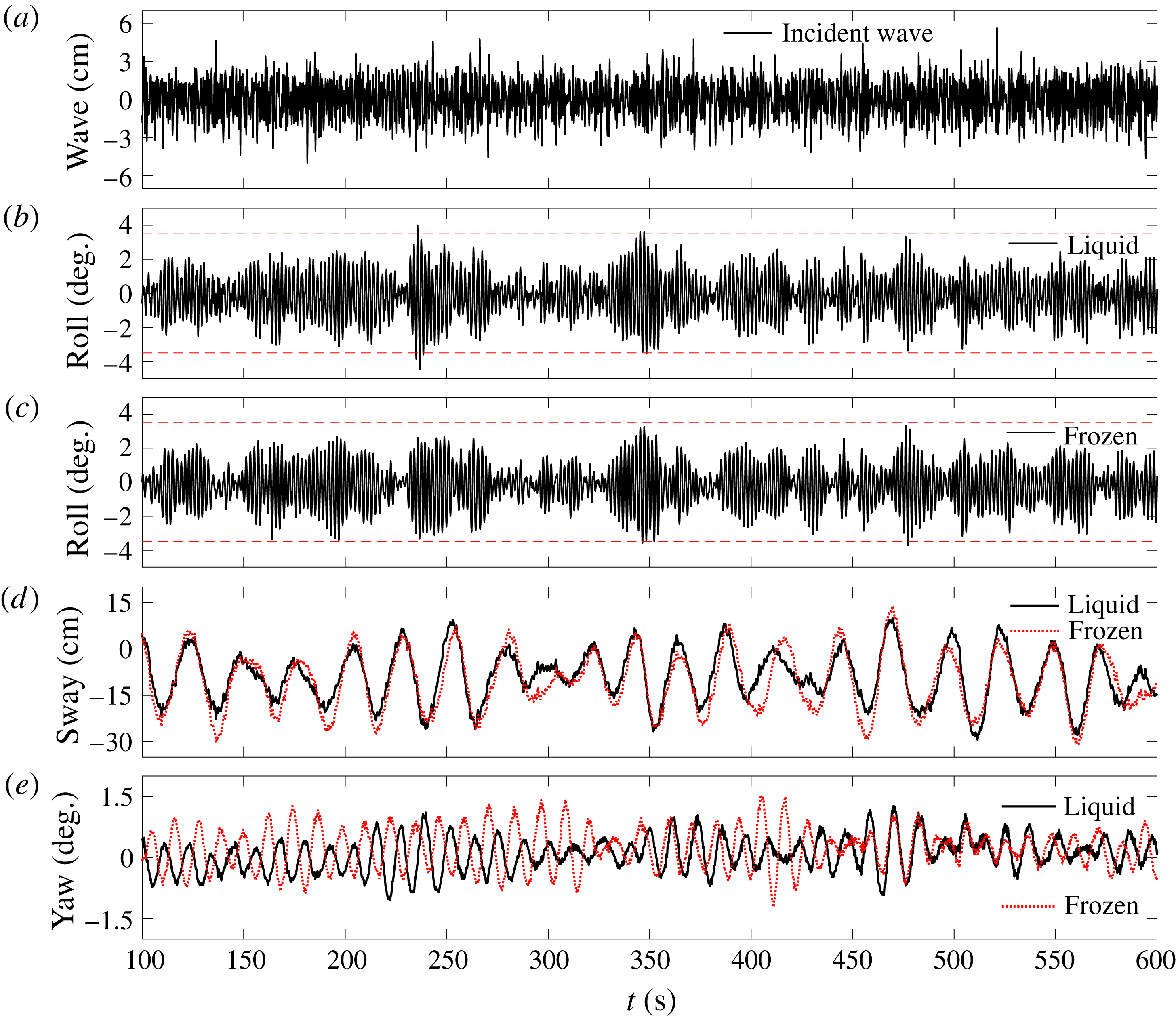
In the model tests, the measurement recording commences as the wavemakers start moving, and continues for 1500 s. The time histories are recorded synchronously for the vessel motions in 6 degrees of freedom and the liquid cargo sloshing inside the spherical tanks. In all cases, we considered only weakly nonlinear uni-directional beam seas. For the 50 % load condition, identical random wave realizations (shown in figure 5 a) excited the model for the liquid and frozen cargo cases. In addition to the roll motions, the sway and yaw motions are also plotted in figure 5, to provide a more comprehensive view of the overall responses of the model carrying partially filled spherical tanks. It should be noted that the time series shown in these figures start after 100 seconds to avoid any effects associated with starting transients, and all the analyses in this study are based on the measured data from 100 s onwards, so 1400 s in total.
Measured time histories for the model at the 50 % load condition: (a) the incident wave elevations, (b,c) comparison between roll in the liquid cargo and frozen cargo cases, (d) comparison between sway in the two cases, (e) comparison between yaw in the two cases.

It is clear in figure 5 that there are visual differences between the wave surface elevation (figure 5
a), which is very broadbanded, and the roll motion (figure 5
b) which shows obvious group structure and looks more narrowbanded. The roll signals for the liquid cargo and the frozen cargo cases are very similar in overall trends. However, the roll amplitudes in the former case are sometimes larger than those in the latter one (horizontal dashed lines are inserted on the plots at
 $\pm 3.5^{\circ }$
to assist the reader). This difference indicates that the extreme roll response may be underestimated if the effects of the liquid cargo are simply ignored. Clearly this could affect estimation of side-by-side offloading availability. It is therefore necessary to explore this phenomenon.
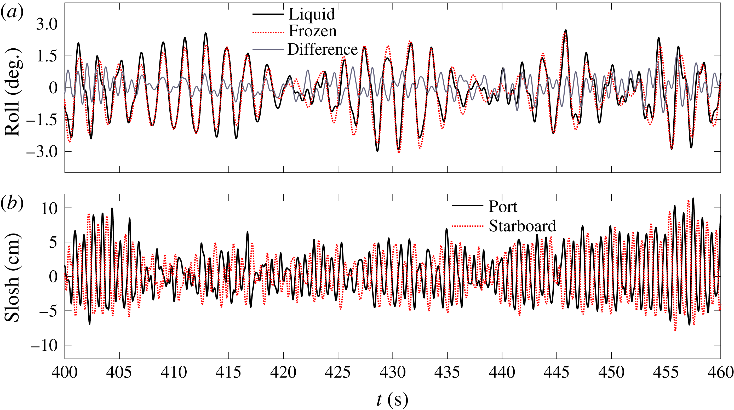
Measured time histories for the model at the 50 % load condition in a selected time window: (a) comparison between roll in the two cases, (b) internal sloshing elevations.

To provide better understanding of the general vessel motions, the sway and yaw (both relative to the long direction of the model, so at
 $0^{\circ }$
to the wave approaching direction in beam seas) are also analysed. As might be expected, figure 5(d) shows obvious slowly varying drift motion of the model for both cases. The model drifts downstream and oscillates in sway slowly around a position 8.11 cm and 9.2 cm away from the original position for the liquid cargo and frozen cargo cases, respectively. Although figure 5(d) shows some local differences, the slowly varying signals are very similar overall. Furthermore, these slight local differences will not affect the main findings in this study, as the slowly varying drift frequency is much smaller than that of the roll response of main interest. Figure 5(e) shows the yaw responses of the models. It is seen that the yaw motion for the model with liquid cargo filled tanks is generally smaller than that for the frozen cargo model. This might be because yaw motions could couple to circumferential sloshing in the two spherical tanks, providing an extra source of motion damping for the liquid filled case. One can see that the yaw responses do not match for the two cases, though it should be noted that the yaw responses in both cases are very small. With broadside uni-directional incident waves and a symmetric model, in principle there should be no yaw motion. The maximum and the standard deviation of the measured yaw responses are very small at around
 $1.5^{\circ }$
and
 $0.4^{\circ }$
respectively, confirming the high quality set-up of the model tests.
To aid visualization of the difference between roll motions with liquid cargo and frozen cargo, we replot a portion of the roll signal in figure 5 over a much smaller time range of 430–460 s in figure 6. The difference signal (liquid–frozen) shows significant higher frequency components. The internal sloshing surface elevations inside one of the spherical tanks is plotted in figure 6(b). The significant asymmetry with respect to the undisturbed water surface indicates the significantly nonlinear nature of the sloshing flow. Detailed discussion will be provided in the following sections.
Although the internal flows are clearly nonlinear, the focus of this study is on the global roll motion accounting for the internal sloshing instead of the nonlinear sloshing flow itself, so we do not attempt detailed analysis of the nonlinear sloshing.
The measured roll signal appears to be relatively narrowbanded, although the input waves are broadbanded. NewWave-type analysis is simple to apply for narrowbanded signals and thus should be able to describe the roll motions well. Similar to our earlier work using NewWave-type methodology (Zhao et al. Reference Zhao, Taylor, Wolgamot and Eatock Taylor2018), we reconstruct a series of NewWave-type groups (with different phases) based on the signal measured in random seas. This allows for further data processing as we did in part 1 (Zhao et al. Reference Zhao, Wolgamot, Taylor and Eatock Taylor2017) where the input waves are deterministic (NewWave-type focused) wave groups.
4 NewWave analysis of the large roll profiles
Prior to conducting the NewWave-type analysis, we first provide the evidence for its applicability for large roll profiles.
4.1 Definition of NewWave
Lindgren (Reference Lindgren1970) and Boccotti (Reference Boccotti1983) showed that the average shape of a large event in any linear random Gaussian process tends to the (scaled) autocorrelation function. This has been described in offshore engineering as NewWave (Tromans et al.
Reference Tromans, Anaturk and Hagemeijer1991; Jonathan & Taylor Reference Jonathan and Taylor1997; Taylor & Williams Reference Taylor and Williams2004; Walker, Taylor & Eatock Taylor Reference Walker, Taylor and Eatock Taylor2004). Thus the linearized average shape (in time) of the large events (the so-called NewWave) is defined to be the scaled autocorrelation function of the measured time history at a particular location. By analogy, the NewWave profile (
 $\unicode[STIX]{x1D711}^{NW}$
) of a roll signal is the inverse Fourier transform of its power spectrum:
 $$\begin{eqnarray}\unicode[STIX]{x1D711}^{NW}=A\cdot \unicode[STIX]{x1D70C}(\unicode[STIX]{x1D70F})=A\cdot \int _{0}^{\infty }S(\unicode[STIX]{x1D714})\cos (\unicode[STIX]{x1D714}\unicode[STIX]{x1D70F})\,\text{d}\unicode[STIX]{x1D714}\bigg/\int _{0}^{\infty }S(\unicode[STIX]{x1D714})\,\text{d}\unicode[STIX]{x1D714},\end{eqnarray}$$
where
 $A$
is the linear ‘crest’ amplitude which may be set to correspond to a certain return period,
 $S(\unicode[STIX]{x1D714})$
is the roll power spectral density,
 $\unicode[STIX]{x1D70F}=t-t_{0}$
is the time relative to the moment when the large value occurs and
 $\unicode[STIX]{x1D70C}$
denotes the autocorrelation function. The variance of the entire random process is defined as:
 $$\begin{eqnarray}\unicode[STIX]{x1D70E}^{2}=\int _{0}^{\infty }S(\unicode[STIX]{x1D714})\,\text{d}\unicode[STIX]{x1D714}.\end{eqnarray}$$
To examine how well the scaled autocorrelation function fits the linearized average shape of the large roll events, it is necessary to estimate confidence intervals. A Lindgren variance (Lindgren Reference Lindgren1970) can be used to asymptotically express the variation in shape of individual ‘crests’ around the expected shape of the scaled autocorrelation function. Far from the time
 $t=0$
, the Lindgren variance reduces to that of the underlying random process. The derivation of the equation for the Lindgren variance is given in his original paper but the result is quoted by Jonathan & Taylor (Reference Jonathan and Taylor1997):
 $$\begin{eqnarray}{\hat{\unicode[STIX]{x1D70E}}_{Li}}^{2}=\unicode[STIX]{x1D70E}^{2}(1-\unicode[STIX]{x1D70C}(\unicode[STIX]{x1D70F})^{2}-\dot{\unicode[STIX]{x1D70C}}(\unicode[STIX]{x1D70F})^{2}\unicode[STIX]{x1D706}^{-2}),\end{eqnarray}$$
where
 $\hat{\unicode[STIX]{x1D70E}}_{Li}$
is the Lindgren standard deviation, and
 $\dot{\unicode[STIX]{x1D70C}}(\unicode[STIX]{x1D70F})$
and
 $\unicode[STIX]{x1D706}$
can be written as below:
 $$\begin{eqnarray}\displaystyle & \displaystyle \dot{\unicode[STIX]{x1D70C}}(\unicode[STIX]{x1D70F})=-\unicode[STIX]{x1D70E}^{-2}\int _{0}^{\infty }\unicode[STIX]{x1D714}S(\unicode[STIX]{x1D714})\sin (\unicode[STIX]{x1D714}\unicode[STIX]{x1D70F})\,\text{d}\unicode[STIX]{x1D714}, & \displaystyle\end{eqnarray}$$
 $$\begin{eqnarray}\displaystyle & \displaystyle \unicode[STIX]{x1D706}^{2}=\unicode[STIX]{x1D70E}^{-2}\int _{0}^{\infty }\unicode[STIX]{x1D714}^{2}S(\unicode[STIX]{x1D714})\,\text{d}\unicode[STIX]{x1D714}. & \displaystyle\end{eqnarray}$$
To provide approximately 5 %–95 % confidence intervals on the expected shape profile, we use
 $\pm 2\unicode[STIX]{x1D70E}_{Li}$
here where
 $\unicode[STIX]{x1D70E}_{Li}$
is the Lindgen standard deviation divided by
 $\sqrt{N-1}$
; i.e. we are looking at the sample variability of the estimated mean compared to the true mean.
4.2 Construction of NewWave profiles – linearization of average shape
The local shape in time around each individual roll response peak is unique. However, it is useful to examine the average shape in time associated with large roll events, by analogy with the treatment of the average shape of large waves measured on the open sea (Jonathan & Taylor Reference Jonathan and Taylor1997; Taylor & Williams Reference Taylor and Williams2004; Santo et al.
Reference Santo, Taylor, Eatock Taylor and Choo2013). The average shape in time is obtained from a given number of the largest roll peaks in the record, here 30 out of a total of
 ${\sim}700$
zero crossings in the 1400 s. By creating shorter time series with each roll maximum point located at relative time
 $t=0$
and then averaging across the short records we produce the so-called NewWave shape. The averaged profiles may then be linearized using harmonic decomposition (Walker et al.
Reference Walker, Taylor and Eatock Taylor2004). This approach is based on the Stokes perturbation expansion. According to the classic Stokes perturbation expansion in the wave slope parameter
 $kA$
, a regular incident wave of linear wave amplitude
 $A$
, frequency
 $\unicode[STIX]{x1D714}$
and wavenumber
 $k$
will induce a response of offshore structures of the following form (up to the second harmonic):
 $$\begin{eqnarray}\unicode[STIX]{x1D711}(\unicode[STIX]{x1D70F})=Af_{1}\cos (\unicode[STIX]{x1D714}\unicode[STIX]{x1D70F})+A^{2}f_{2}\cos (2\unicode[STIX]{x1D714}\unicode[STIX]{x1D70F}+\unicode[STIX]{x1D713}).\end{eqnarray}$$
The phase-inversion method (Jonathan & Taylor Reference Jonathan and Taylor1997) can be used to separate the linearized profile and the second harmonic, with the assumption that the higher harmonic contributions are negligible. In this method, two time series which are
 $180^{\circ }$
out of phase are needed. The idea is that the phase shift will cause the signs of the odd harmonics to change, so the components are inverted while those of the even harmonics remain unaltered. As a consequence, the linear and second harmonic components of the average shape of extreme roll events can be extracted.
 $$\begin{eqnarray}\displaystyle & \displaystyle \unicode[STIX]{x1D711}^{L}\approx \unicode[STIX]{x1D711}^{odd}={\textstyle \frac{1}{2}}(\overline{\unicode[STIX]{x1D711}}_{+}-\overline{\unicode[STIX]{x1D711}}_{-}), & \displaystyle\end{eqnarray}$$
 $$\begin{eqnarray}\displaystyle & \displaystyle \unicode[STIX]{x1D711}^{S}\approx \unicode[STIX]{x1D711}^{even}={\textstyle \frac{1}{2}}(\overline{\unicode[STIX]{x1D711}}_{+}+\overline{\unicode[STIX]{x1D711}}_{-}), & \displaystyle\end{eqnarray}$$
where
 $\overline{\unicode[STIX]{x1D711}}_{+}$
is the average of the large (max. downwave) roll responses of any point above the roll centre and
 $\overline{\unicode[STIX]{x1D711}}_{-}$
is the average of the large upwave response of any point above the roll centre. By analogy with surface wave analysis, we (arbitrarily) denote maximum downwave motion events in time as crests (so
 $+$
), and upwave motion events as troughs (so
 $-$
).
4.3 Comparison between constructed NewWave and scaled autocorrelation function
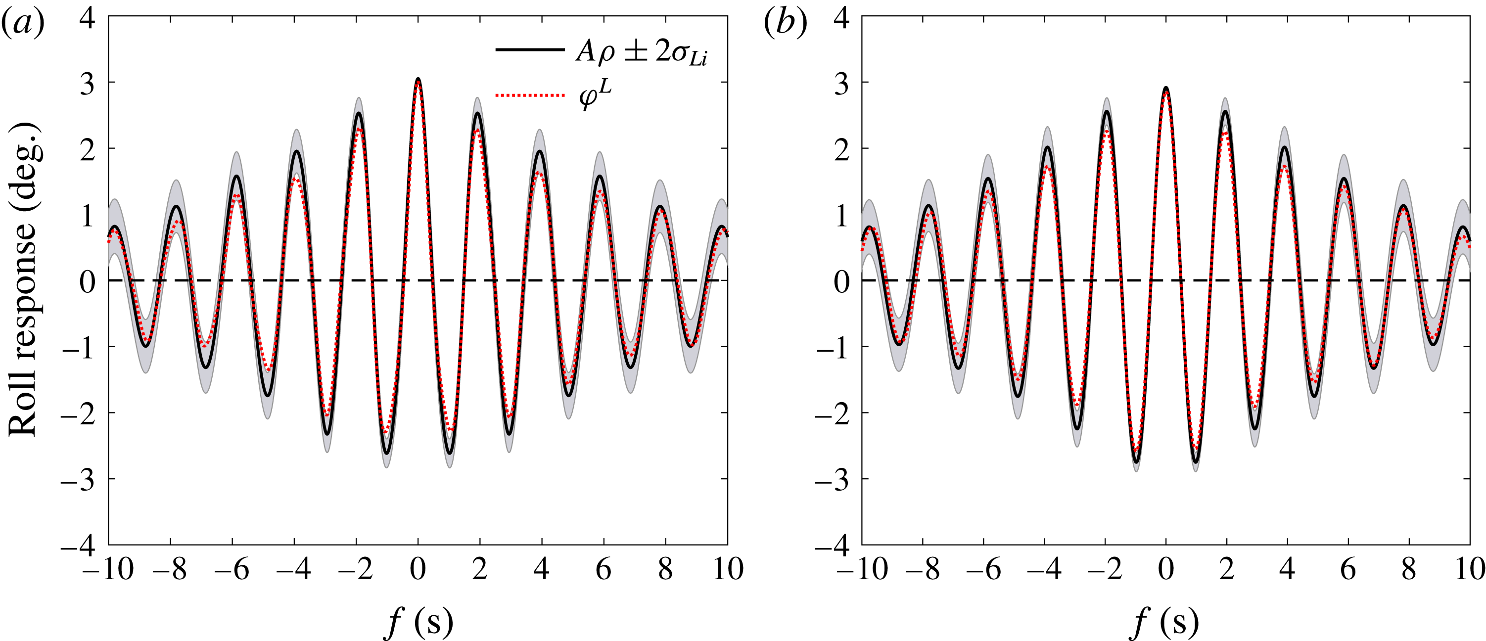
Comparisons of the scaled autocorrelation function and the constructed NewWave profile have been plotted, together with the approximately 5 %–95 % confidence intervals of the mean. Figure 7 shows the results for the liquid and frozen cargo cases, where the grey ‘band’ shows the confidence interval (
 $A\unicode[STIX]{x1D70C}+2\unicode[STIX]{x1D70E}_{Li}$
to
 $A\unicode[STIX]{x1D70C}-2\unicode[STIX]{x1D70E}_{Li}$
). It can be seen that for both the liquid and the frozen cargo cases, the scaled autocorrelation function (
 $A\unicode[STIX]{x1D70C}$
) fits the constructed NewWave profile (
 $\unicode[STIX]{x1D711}^{NW}$
) of the measured roll motions, which is obtained using a two-phase decomposition method, i.e.
 $\unicode[STIX]{x1D711}^{NW}=\unicode[STIX]{x1D711}^{L}$
(see (4.7)). So we conclude that NewWave is a reasonable model for the linear part of the largest roll responses in random waves, both with and without liquid cargo effects.
Ability of the scaled autocorrelation function (
 $A\unicode[STIX]{x1D70C}$
) to represent the linearized average shape (
 $\unicode[STIX]{x1D711}^{L}$
) of the large roll responses of the model at the 50 % load condition: (a) liquid cargo case, (b) frozen cargo case.

5 High-order harmonics and coupling
Spectral analyses are conducted for the measured roll signals, showing a secondary peak in addition to the main roll resonant response. To explore nonlinear contributions to this phenomenon and explore the effects of liquid cargo flow on the global roll response, higher harmonics are isolated and analysed. Then, the coupling between harmonics of the main roll resonant response and internal sloshing is investigated.
5.1 Spectral analysis of the measured signals
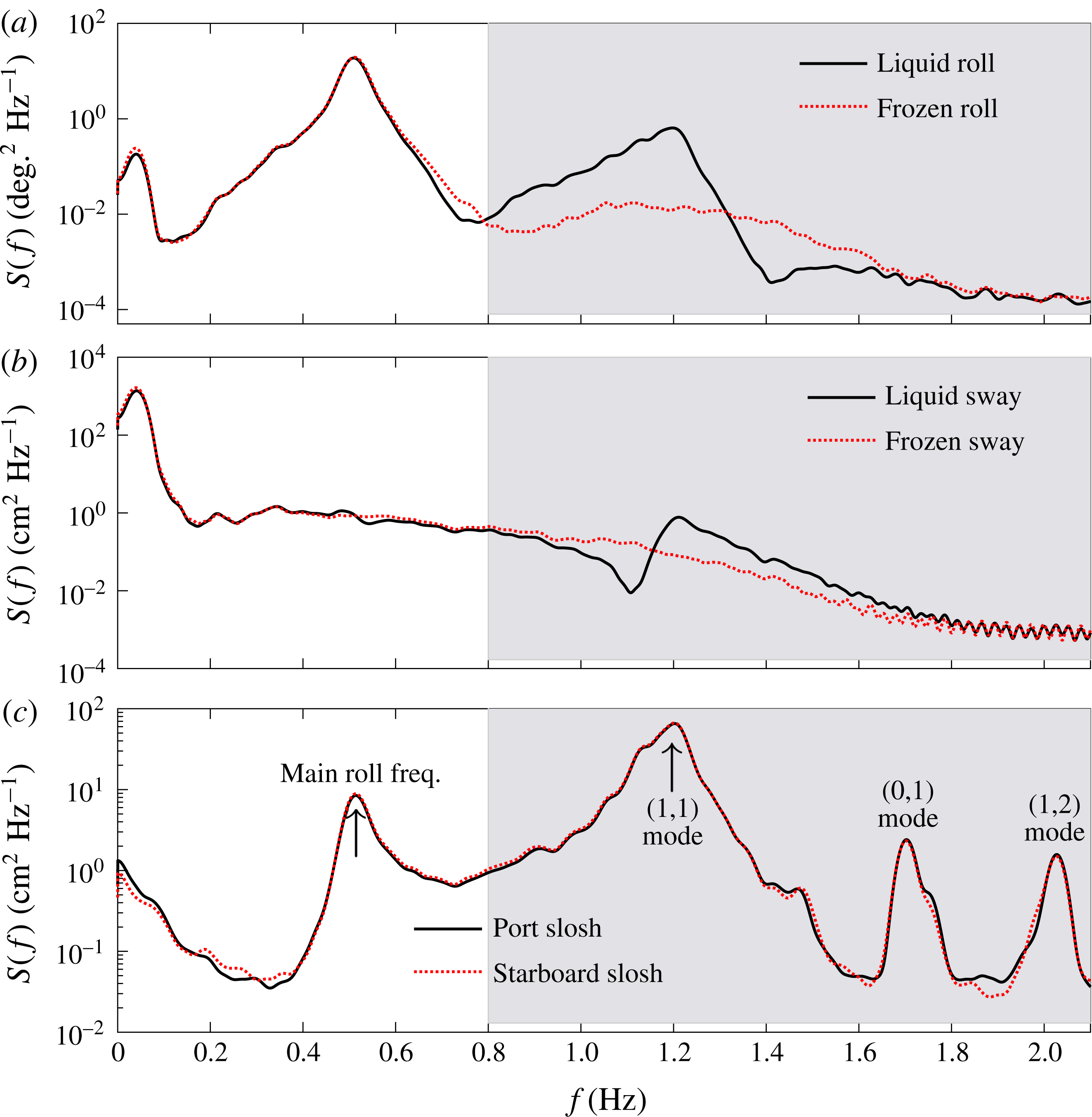
The power spectra of the roll motion signals for the liquid and frozen cargo cases, and for internal sloshing and sway motions are studied. An observable but small response peak at a frequency below 0.1 Hz is observed for the roll motions in both the liquid cargo and frozen cargo cases. This is associated with slow drift motions in the horizontal plane (i.e. sway motions) shown in figure 8(b). The principal mode of response at
 ${\sim}0.5$
Hz corresponds to the linear roll resonance of the model. Higher frequency harmonic components of the roll responses in the frozen cargo case are very small, but in the liquid cargo case one can observe a marked secondary peak in the roll response at around 1.2 Hz. We do not observe any significant nonlinear roll damping in these tests, of a Morison drag-type form. This is presumably because the roll motion is not large enough to cause significant flow separation at the bilge keels. At model scale there will be linear Stokes oscillatory boundary type damping, comparable to that observed in Zhao et al. (Reference Zhao, Wolgamot, Taylor and Eatock Taylor2017) for the gap resonance problem.
Power spectra of the measured signals with the model at the 50 % load condition, the vertical axes are on log scales. (a) Roll motions, (b) sway motions, (c) sloshing with the frequencies of the different slosh modes marked. The spectra are split at the minimum of the liquid roll response, where the grey shading is used to denote the high pass signal components and the unshaded white area the low pass signal components.

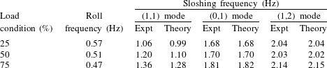
The natural frequencies of sloshing modes in the spherical tanks under different load conditions were determined by identifying spectral peaks. These may also be estimated using the results of McIver (Reference McIver1989) or Faltinsen & Timokha (Reference Faltinsen and Timokha2009, Reference Faltinsen and Timokha2012). The results are listed in table 2, together with the natural frequencies of the global roll response at different load conditions. The measured sloshing frequencies match the analytical approximations extremely well, apart from the (1,1) mode (the lowest mode by frequency for spherical tanks) where the measured frequencies are slightly upshifted for all three load conditions. This phenomenon is believed to be associated with the interactions possible in a linear 2 degrees-of-freedom system, where the degrees in this case are the global roll motions and the (1,1) sloshing mode. This is discussed further in appendix A.
Natural frequencies for roll motions and internal fluid sloshing (at laboratory scale). ‘Expt’ refers to the measured frequencies of the sloshing modes, ‘Theory’ the analytical approximation based on Faltinsen & Timokha (Reference Faltinsen and Timokha2009, Reference Faltinsen and Timokha2012).

Figure 8(c) shows that the most severe sloshing in the 50 % full case occurs at the lowest sloshing mode (the (1,1) mode) frequency of 1.2 Hz, which is well above 0.5 Hz where the main roll response occurs. The response peaks around 1.7 Hz and 2.0 Hz in figure 8(c) suggest that other sloshing modes (e.g. (0,1) and (1,2) modes) are also excited, although the response amplitudes are much smaller than that of the (1,1) mode. The other sloshing modes may have larger amplitudes when their frequencies coincide with harmonics of the (1,1) mode – this occurs for specific filling levels larger than 50 % (Faltinsen & Timokha Reference Faltinsen and Timokha2013a ,Reference Faltinsen and Timokha b ), which do not coincide with the 75 % volume fill level tested here. Here, our focus is on global roll motions, which do not seem to be affected by the sloshing in other modes – see figure 8(a) – in line with expectation given the mode shapes for these modes (Faltinsen & Timokha Reference Faltinsen and Timokha2012).
5.2 Extraction of higher harmonics – conditioned signal analysis
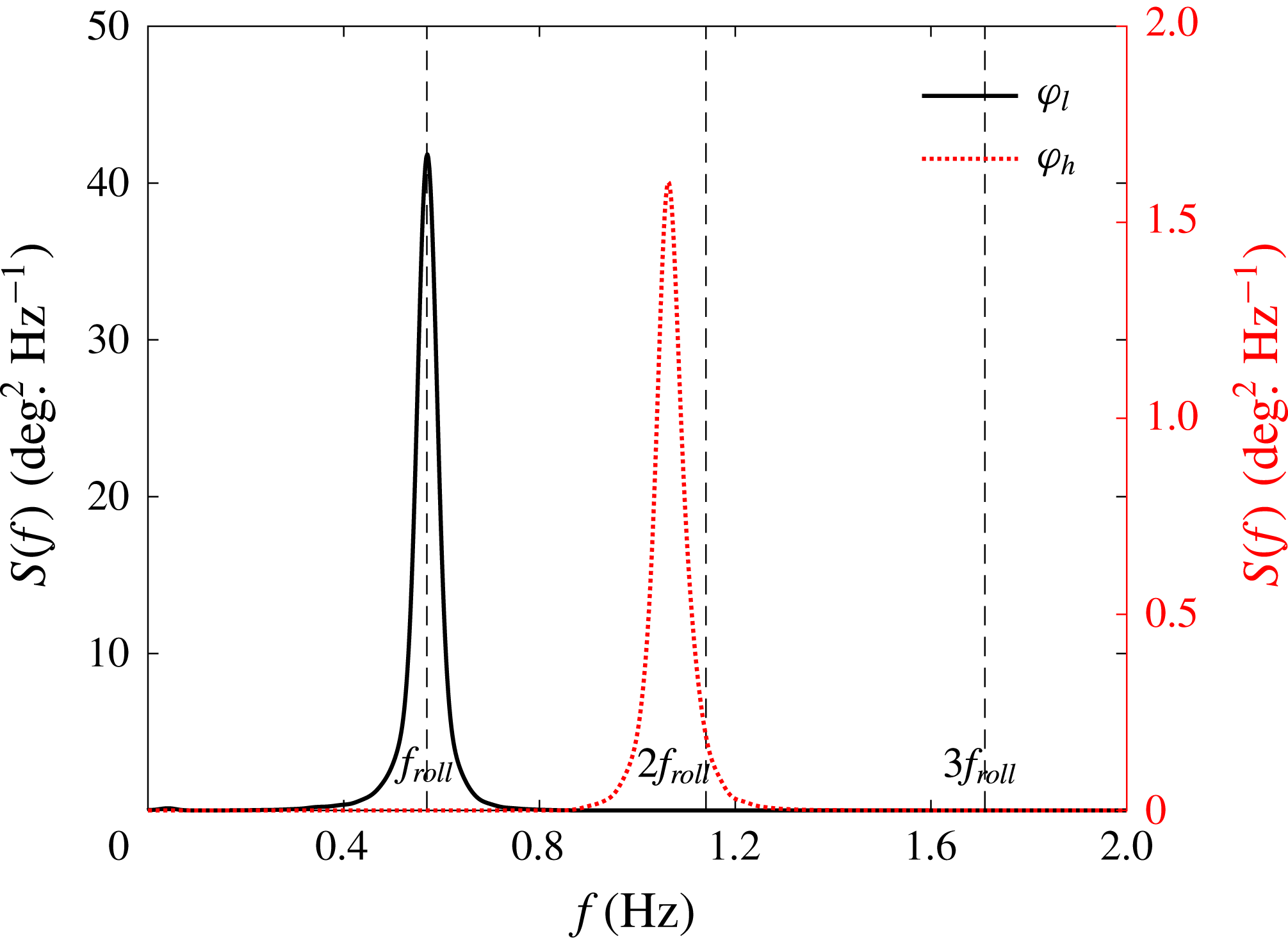
To explore any nonlinear coupling between higher harmonics of the main roll resonance and the (1,1) mode sloshing, the roll response at the 50 % load condition was bandpass filtered at 0.80 Hz, forming two time series designated low pass and high pass components, as indicated in figure 8. For comparison purposes, this was also done for the roll responses at the same load condition but with frozen cargo. The roll responses at the 25 % and 75 % load conditions were analysed in a similar method but only for the case with liquid cargo inside the tanks. The relevant bandpass frequencies were 0.88 Hz and 0.72 Hz, respectively, for these two fill levels.
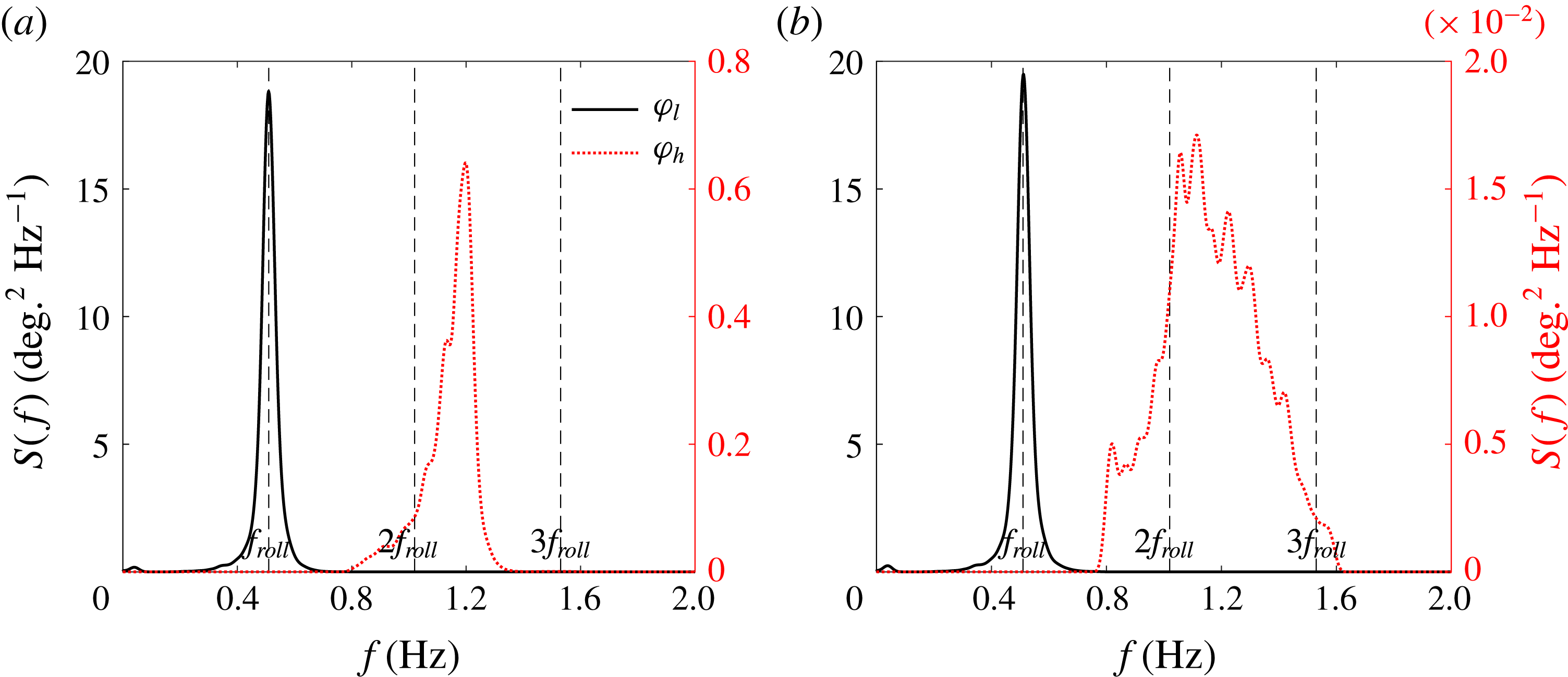
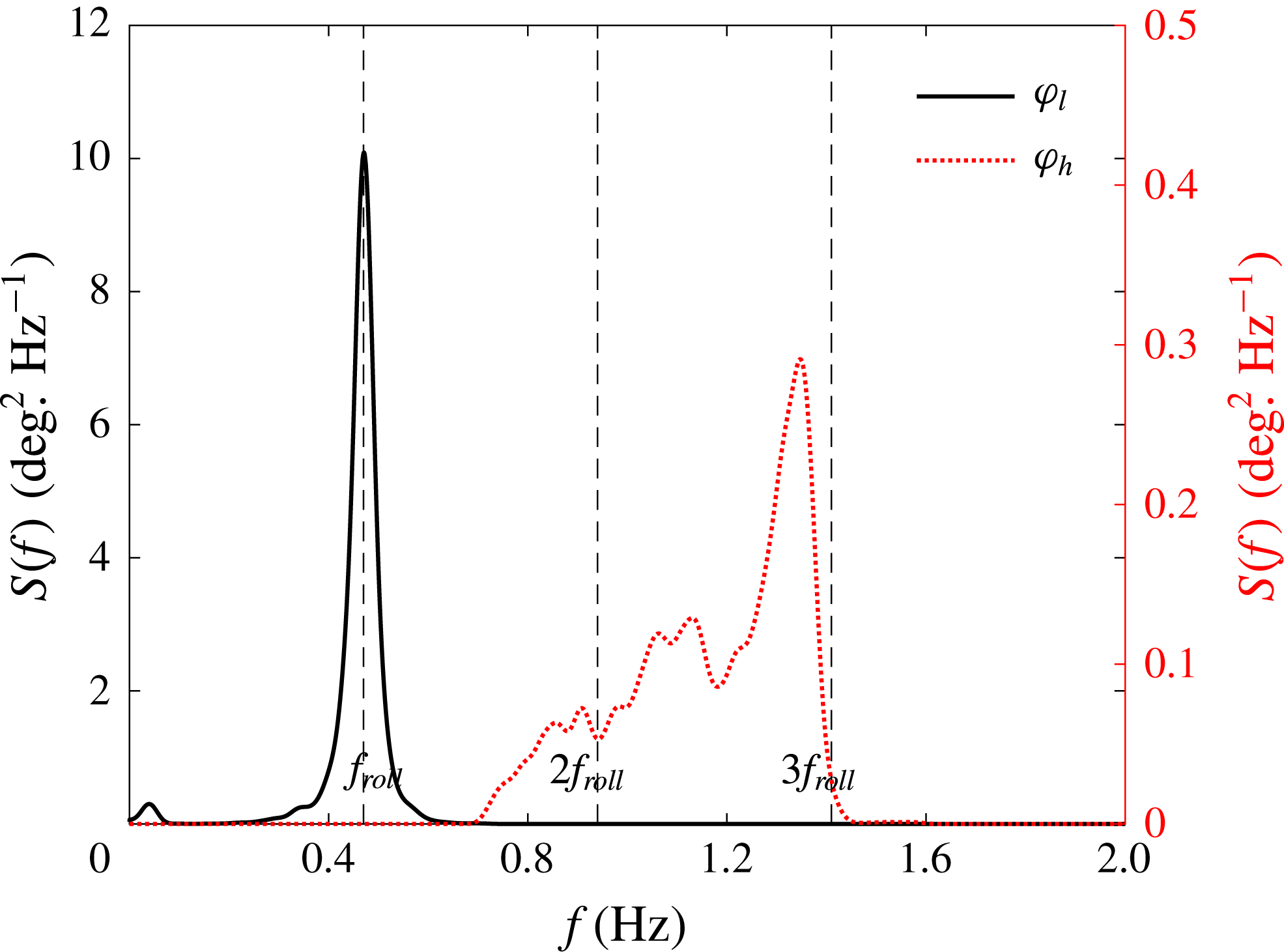
Response spectra of the filtered roll motions at the 50 % load condition: (a) vessel model with liquid cargo, (b) vessel model with frozen cargo.
 $\unicode[STIX]{x1D711}_{l}$
and
 $\unicode[STIX]{x1D711}_{h}$
refer to the low and high pass signal respectively. Note the different scales for the high pass component between (a) and (b).
 $f_{roll}$
refers to the natural frequency of the linear roll motion.

After splitting the roll response of the carrier model at the 50 % load condition into two frequency components as indicated in figure 8, spectral analysis was conducted for each. Figure 9(a) shows the spectra of the low pass and high pass signals for the cases with liquid cargo. We assume the high pass signal could be driven linearly or by higher harmonics. For comparison, figure 9(b) shows the same results but for the carrier model with frozen cargo.
A secondary roll peak occurs at double the frequency of the main resonant roll motion for the case with frozen cargo. However, it is very small compared to the liquid cargo case. Since there is no liquid cargo in the frozen cargo case, this minor secondary response peak is believed to be a result of both small linear excitation by high frequency waves and more likely a double frequency quadratic coupling effect. The power spectrum for the low pass roll signal for the liquid fill case shown in figure 9(a) has a simple shape, being smooth and symmetric, while the high pass roll signal exhibits more structure (wiggles in the spectrum).
5.2.1 Signal processing methods
It is obvious that extracting higher and particularly nonlinear harmonics is difficult in a broadbanded random sea. Simple frequency filtering is inadequate. To pursue a general approach to investigating nonlinear coupling from low to high frequency, a four-phase combination method (Fitzgerald et al.
Reference Fitzgerald, Taylor, Eatock Taylor, Grice and Zang2014) based on weakly nonlinear theory is adopted. The four-phase combination method is the same idea as the two-phase method described in § 4.2, but enables the separation of the first four harmonics. In the present case we are not extracting the harmonics of the total signal but extracting the harmonics of one (high frequency) part of the signal which are coupled to another (low frequency) part. This requires separating the frequency content into separate signals by filtering and then conditioning the high pass signal on the low pass to make sure that we can distinguish between coupled and uncoupled responses. In this work by ‘signal
 $X$
conditioned on signal
 $Y$
’ we mean that we have selected the
 $N$
parts of signal
 $X$
that occur at the same times as some
 $N$
similar events occur in signal
 $Y$
, the signals being recorded synchronously. By averaging the
 $N$
parts of signal
 $X$
we reduce those parts with no phase relationship (coupling) to the average event in signal
 $Y$
to the level of background noise, so that we may then extract the coupled harmonics.
Details of the four-phase approach are given in Fitzgerald et al’s paper, but we provide a summary here. We start by assuming a nonlinear response (say the roll motion
 $\unicode[STIX]{x1D711}$
) can be written as a Stokes-like series to
 $O(A^{4})$
in amplitude and to the fourth harmonic in frequency:
 $$\begin{eqnarray}\displaystyle \unicode[STIX]{x1D711}_{(0)} & = & \displaystyle Af_{11}\cos (\unicode[STIX]{x1D703})+A^{2}(f_{20}+f_{22}\cos 2\unicode[STIX]{x1D703})+A^{3}(f_{31}\cos \unicode[STIX]{x1D703}+f_{33}\cos 3\unicode[STIX]{x1D703})\nonumber\\ \displaystyle & & \displaystyle +\,A^{4}(f_{40}+f_{42}\cos 2\unicode[STIX]{x1D703}+f_{44}\cos 4\unicode[STIX]{x1D703})+O(A^{5}).\end{eqnarray}$$
Now we create phase shifted forms of this function, the phase shifts being
 $90^{\circ }$
,
 $180^{\circ }$
(equivalent to changing the sign of
 $A$
) and
 $270^{\circ }$
. Thus
 $\cos (\unicode[STIX]{x1D703})$
is replaced by
 $\cos (\unicode[STIX]{x1D703}+90^{\circ })=-\sin (\unicode[STIX]{x1D703})$
,
 $\cos (2\unicode[STIX]{x1D703})$
by
 $\cos (2\unicode[STIX]{x1D703}+180^{\circ })=-\cos (2\unicode[STIX]{x1D703})$
, etc. In deterministic physical experiments such as wave groups in a wave tank, the phase of the linear component of the input waves is immediately accessible through the paddle control software. This basic four-phase method has been adopted successfully to extract the higher harmonics in our previous study on gap resonance in focused wave groups – part 1 (Zhao et al.
Reference Zhao, Wolgamot, Taylor and Eatock Taylor2017). The method of constructing NewWave-type wave groups (with different phases) from random responses has been illustrated in part 2 (Zhao et al.
Reference Zhao, Taylor, Wolgamot and Eatock Taylor2018).
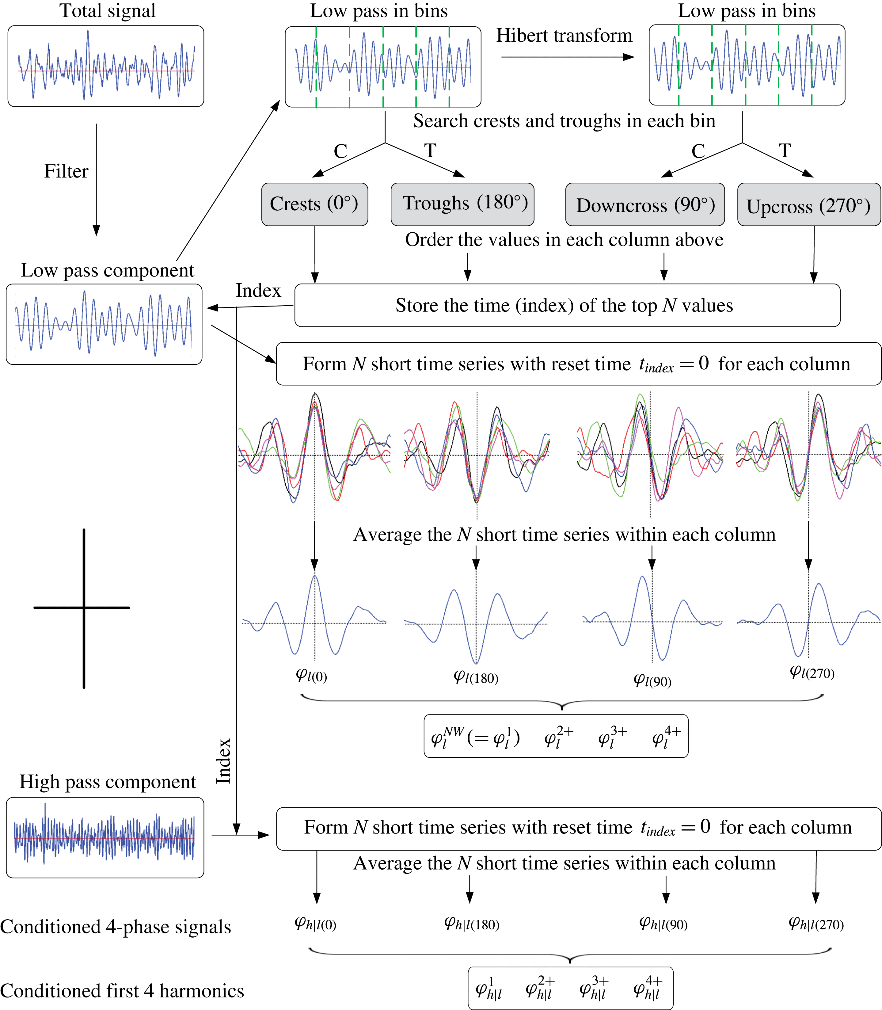
Illustration of the NewWave-type analysis based on conditioning process used to analyse the high and low pass components.
 $\unicode[STIX]{x1D711}_{l}^{NW}$
refers to the NewWave profiles of the low pass signal, and
 $\unicode[STIX]{x1D711}_{h|l}$
(short for
 $\unicode[STIX]{x1D711}_{h}|\unicode[STIX]{x1D711}_{l}^{NW}$
) the (high pass) signal profiles conditioned on the low pass term. Hence, for
 $\unicode[STIX]{x1D711}_{h|l(0)}$
, we find the local average shape of the high pass component around the time at which the low pass component has a large crest. The subscripts ‘0’, ‘90’, ‘180’ and ‘270’ refer to the phase, and ‘1’, ‘2+’, ‘3+’ and ‘4+’ the first hour harmonics obtained based on the four-phase signal.

Here we go one step further by introducing a conditioning process when constructing the NewWave-type wave groups illustrated in part 2. The harmonic separation equations are given as:
 $$\begin{eqnarray}\displaystyle & \displaystyle \unicode[STIX]{x1D711}_{h|l}^{1}\approx (f_{11}A+f_{31}A^{3})\cos \unicode[STIX]{x1D703}={\textstyle \frac{1}{4}}(\unicode[STIX]{x1D711}_{h|l(0)}-\unicode[STIX]{x1D711}_{h|l(90)}^{H}-\unicode[STIX]{x1D711}_{h|l(180)}+\unicode[STIX]{x1D711}_{h|l(270)}^{H}), & \displaystyle\end{eqnarray}$$
 $$\begin{eqnarray}\displaystyle & \displaystyle \unicode[STIX]{x1D711}_{h|l}^{2+}\approx (f_{22}A^{2}+f_{42}A^{4})\cos 2\unicode[STIX]{x1D703}={\textstyle \frac{1}{4}}(\unicode[STIX]{x1D711}_{h|l(0)}-\unicode[STIX]{x1D711}_{h|l(90)}+\unicode[STIX]{x1D711}_{h|l(180)}-\unicode[STIX]{x1D711}_{h|l(270)}), & \displaystyle\end{eqnarray}$$
 $$\begin{eqnarray}\displaystyle & \displaystyle \unicode[STIX]{x1D711}_{h|l}^{3+}\approx f_{33}A^{3}\cos 3\unicode[STIX]{x1D703}={\textstyle \frac{1}{4}}(\unicode[STIX]{x1D711}_{h|l(0)}+\unicode[STIX]{x1D711}_{h|l(90)}^{H}-\unicode[STIX]{x1D711}_{h|l(180)}-\unicode[STIX]{x1D711}_{h|l(270)}^{H}), & \displaystyle\end{eqnarray}$$
 $$\begin{eqnarray}\displaystyle & \displaystyle \unicode[STIX]{x1D711}_{h|l}^{4+}\approx f_{44}A^{4}\cos 4\unicode[STIX]{x1D703}={\textstyle \frac{1}{4}}(\unicode[STIX]{x1D711}_{h|l(0)}+\unicode[STIX]{x1D711}_{h|l(90)}+\unicode[STIX]{x1D711}_{h|l(180)}+\unicode[STIX]{x1D711}_{h|l(270)}), & \displaystyle\end{eqnarray}$$
where the superscript
 $H$
refers to the Hilbert transform of the signal;
 $\unicode[STIX]{x1D711}_{h|l}$
(short for
 $\unicode[STIX]{x1D711}_{h}|\unicode[STIX]{x1D711}_{l}^{NW}$
) indicates the high pass (roll) signals conditioned on extrema in the low pass (roll) signals; and the subscripts (0, 90, 180 and 270) in brackets represent the shifted phase of the conditioning signals, respectively. The fourth linear combination (5.5) is slightly simpler than that given by Fitzgerald et al. (Reference Fitzgerald, Taylor, Eatock Taylor, Grice and Zang2014), since we ignore any second-order difference harmonic response term. This term was removed when conducting the frequency filtering in the present study. This harmonic separation technique allows us to separate the first four harmonics, based on a large crest (
 $0^{\circ }$
), downcrossing (
 $90^{\circ }$
), trough (
 $180^{\circ }$
) and upcrossing (
 $270^{\circ }$
), where the downcrossing and upcrossing signals are extracted by finding the maximum and minimum points of the Hilbert transformed (
 $90^{\circ }$
phase shifted) low pass components. All the necessary signal processing was performed in MATLAB.
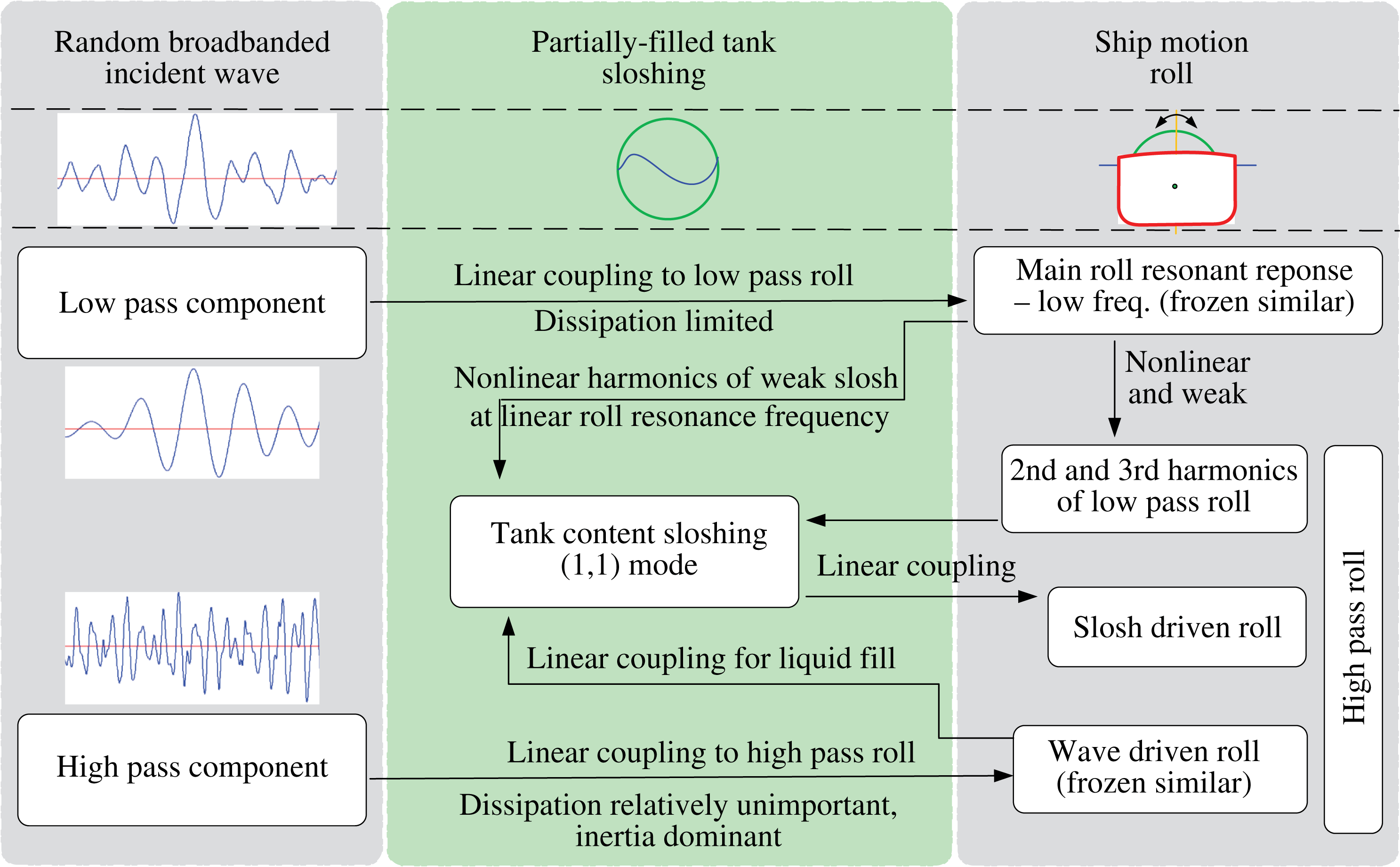
To provide a clearer explanation of the conditioning process and the signals used for four-phase harmonic separation, we summarize the procedure in the flowchart in figure 10.
5.2.2 Results for the 50 % load condition
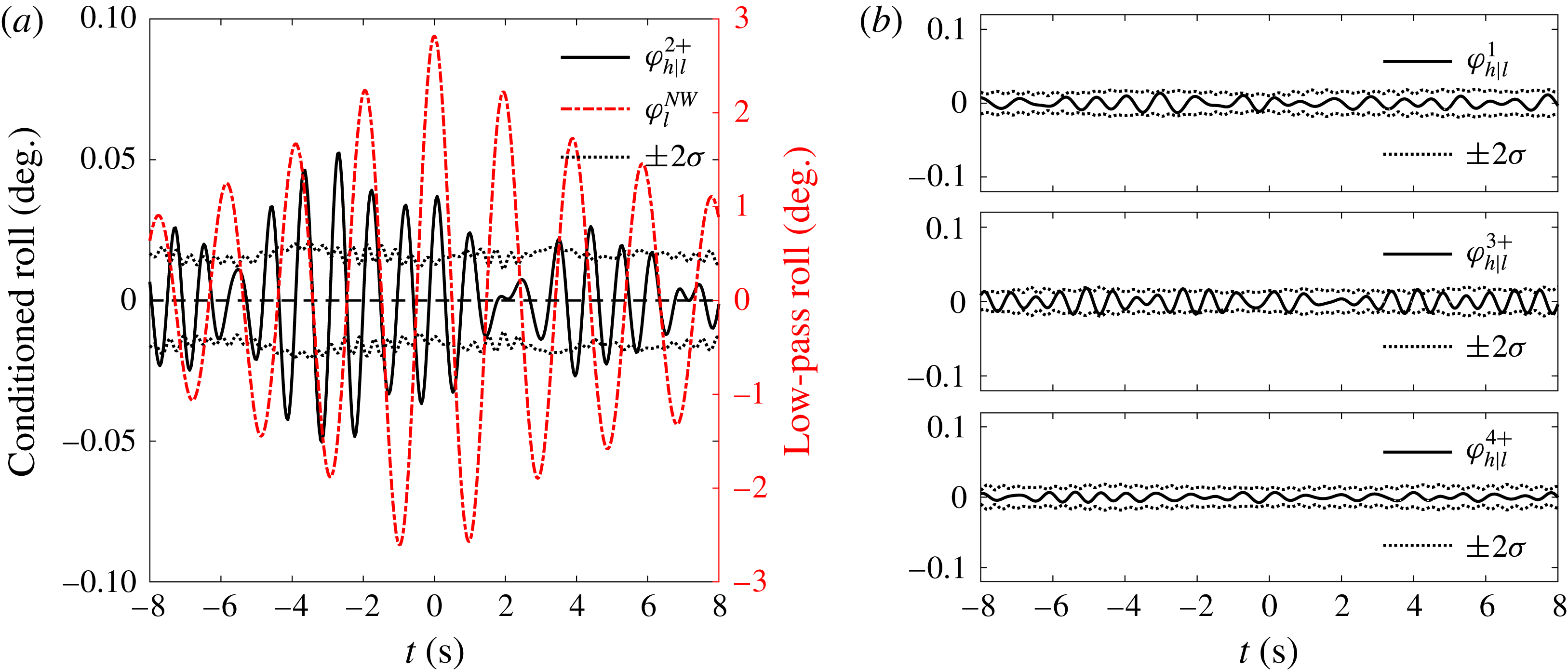
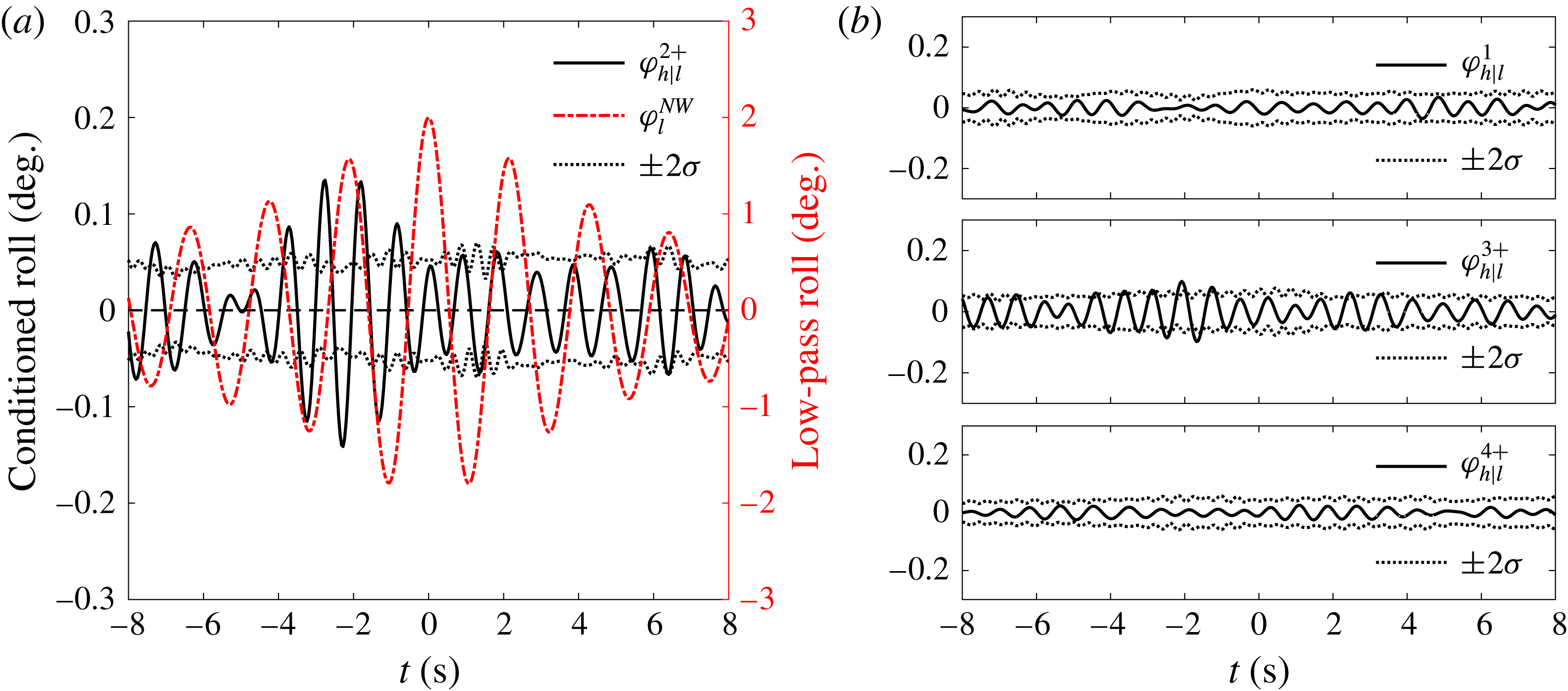
The results of the four-phase separation using conditioned roll signals for the model at the 50 % load condition with frozen cargo are shown in figure 11. Evidently, the first harmonic signal (b, top) is very small and negligible compared with the second harmonic (a, black solid line). This is because we are looking at the high pass signal where the roll driven linearly around the roll natural frequency has already been filtered out. The first, third and fourth harmonics are obviously within the error bars computed as approximately 5 %–95 % confidence intervals on the estimation of the mean signal, so are simply noise. There are no visible higher harmonics in conditioned high frequency roll, except the second harmonic contribution with a magnitude of
 $0.05^{\circ }$
, which is very small. The averaged low pass linear roll signal, used to condition the averaged high pass components is shown as the red signal in figure 11(a). The vertical label in the centre of the figure in red corresponds to the axis for the linear roll signal.
Harmonic separation of the high pass roll signal conditioned on the low pass roll signal for the 50 % load condition with frozen cargo in tanks.
 $\unicode[STIX]{x1D711}_{l}^{NW}$
refers to the NewWave profile of the low pass roll signal, and
 $\unicode[STIX]{x1D711}_{h|l}^{2+}$
is short for
 $\unicode[STIX]{x1D711}_{h}^{2+}|\unicode[STIX]{x1D711}_{l}^{NW}$
, the second harmonic of the high pass roll signal conditioned on
 $\unicode[STIX]{x1D711}_{l}^{NW}$
.

Figure 12 shows the same results as in figure 11 but for the model at the 50 % load condition with liquid cargo. The first, third and fourth harmonics are again much smaller than the second harmonic and within the error bars, so are probably just signal leakage. This result indicates that the second harmonic is the dominant coupled nonlinearity for the liquid cargo condition. In general, the harmonic separation presented in figure 12 appears to have significant double frequency harmonics and perhaps some visible triple frequency harmonics.
It should be noted that we are using conditioning on peaks in the low pass signal to search for nonlinear coupling to the high frequency signal. The internal sloshing frequency (1.20 Hz) is between 2 times the frequency of the main roll signal (1.02 Hz) and 3 times the frequency of the main roll signal (1.53 Hz), so we might expect nonlinear coupling from the internal fluid sloshing modes into the high pass roll signal. This will be discussed in detail in § 6. To examine whether the observation in this section is given by chance for only this load condition, studies for the other two load conditions, namely 25 % and 75 %, are addressed next.
5.2.3 Results for the 25 % load condition
As for the case of the 50 % load condition, the roll response signal of the carrier model at the 25 % load condition with liquid cargo only is filtered into two parts below and above a frequency cutoff (in this case 0.88 Hz).
The spectra of the low pass and high pass signals are plotted in figure 13. Both the low pass and the high pass spectral peaks have a simple form, being smooth and symmetric. The high pass signal is relatively a little more broadbanded than the low pass signal.
As in figure 11, but for the 50 % load condition with liquid cargo in tanks.

Response spectra of the filtered roll motions at the 25 % load condition with liquid cargo in tanks.

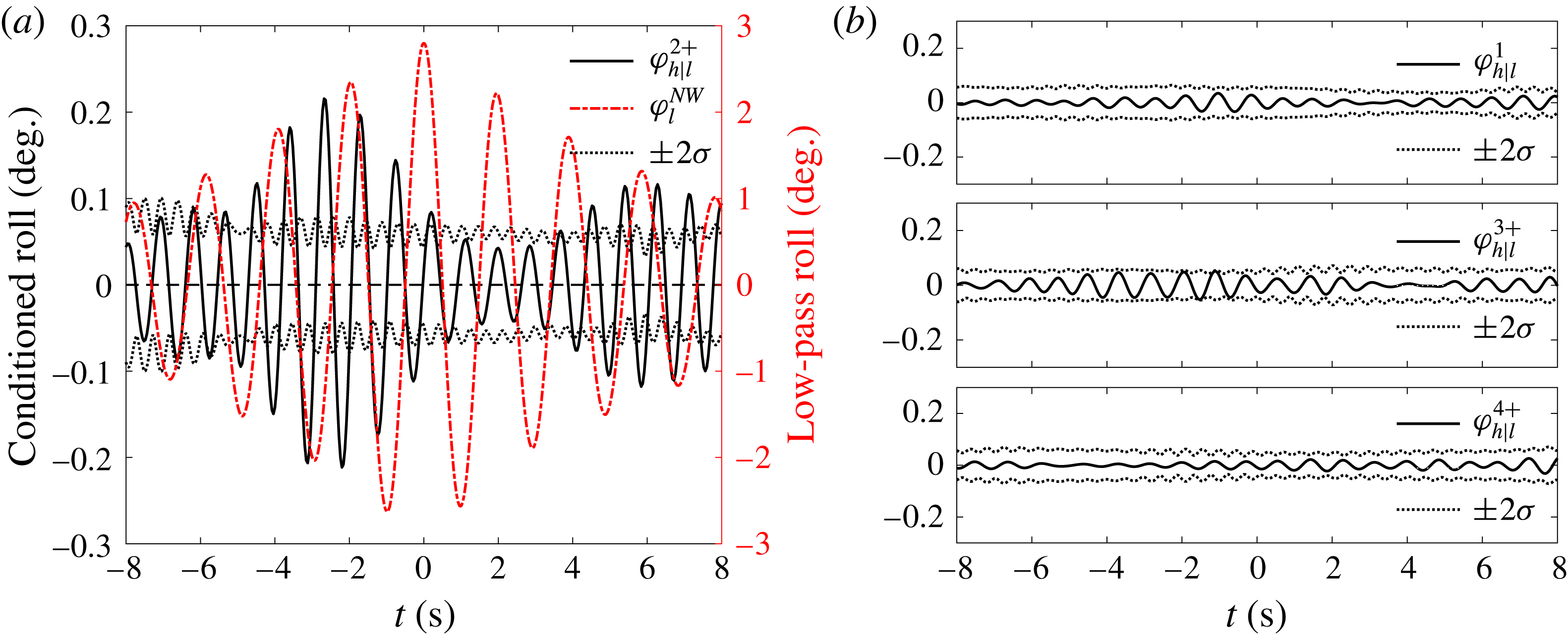
Four-phase separation is conducted for the roll signals of the model at 25 % load condition with liquid cargo, based on the conditioning process (as shown in figure 10). Figure 14 shows the first four harmonics of the high frequency roll signals conditioned on the low pass roll signals.
As in figure 12, but for the 25 % load condition with liquid cargo in tanks.

The amplitudes of the first, third, and fourth harmonics are approximately
 $1/10$
th of the second harmonic. So we can conclude that the second harmonic is the dominant coupled nonlinearity. One can note that the first, third, and fourth harmonics show almost the same number of peaks and troughs as the second harmonic, indicating that there is leakage from the second harmonic and that the first, third, and fourth harmonics are not the exact four-phase combinations. This is because we are dealing with a finite number of random signals (here 30) instead of the carefully controlled localized wave groups of Fitzgerald et al. (Reference Fitzgerald, Taylor, Eatock Taylor, Grice and Zang2014) and Zhao et al. (Reference Zhao, Wolgamot, Taylor and Eatock Taylor2017), where cancellation would be much better.
The sloshing frequency (1.06 Hz) is very close to 1.14 Hz which is 2
 $\times$
the frequency of the main roll signal (0.57 Hz), so we would expect coupling from the sloshing mode in the high pass signal. By using the conditioning and averaging we expect to avoid any linear excitation of the internal sloshing by wave action at this frequency (1.06 Hz), because there would be no direct coupling between the linear wave components at high frequency and the linear low pass waves (except if the frequency excitation is exactly a factor of 2 apart). With a conditioned low pass roll of approximately
 $4^{\circ }$
, we obtain a correlated double frequency roll of around
 $0.25^{\circ }$
. Hence the high frequency sloshing back-reacts on the model roll and the contribution is approximately 6 % of the low pass roll.
5.2.4 Results for the 75 % load condition
As for the previous cases, the roll signals of the model at the 75 % load condition with liquid cargo is bandpass filtered into two parts (in this case, cut at a frequency of 0.72 Hz).
The spectra of the low pass and high pass signals are shown in figure 15. It can be seen that the high pass signal is relatively much more broadbanded than the low pass signal. One can see from the shape that the spectrum seems to consist of two components with different frequencies, which can be further clarified from the four-phase combination separation results next.
Response spectra of the filtered roll motions at the 75 % load condition with liquid cargo in tanks.

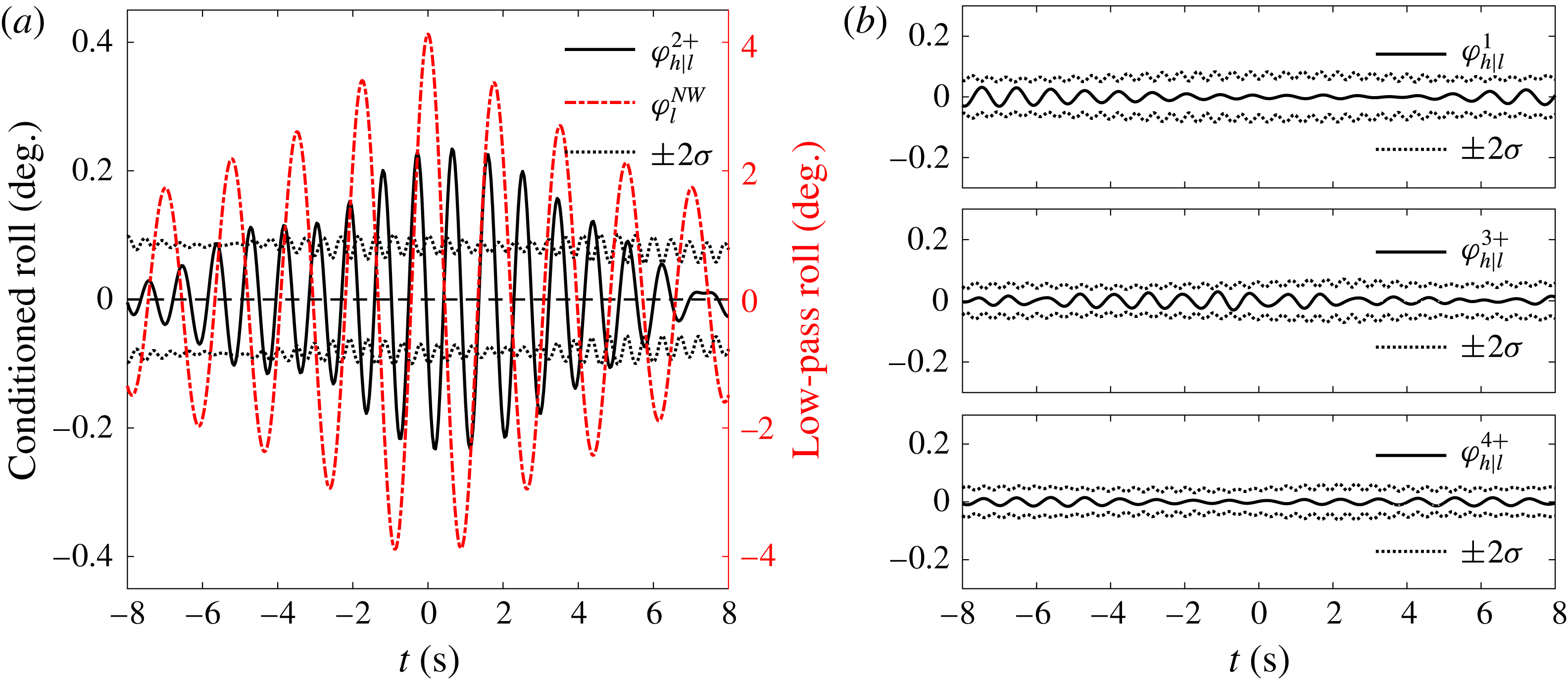
The first four harmonics of the conditioned roll signals based on four-phase separation are obtained, for the 75 % load condition with liquid cargo. As shown in figure 16, the first and fourth harmonic conditioned signals are just
 $1/10$
th of the second harmonic, but the third harmonic is larger (extends beyond the error bars) and is approximately 75 % of the size of the second harmonic. So the first and fourth conditioned signals are presumably the result of signal leakage, but the third conditioned signal is significant. It is clear that the double frequency and triple frequency harmonics contribute to roll for the 75 % load condition.
As in figure 12, but for the 75 % load condition with liquid cargo in tanks.

At the 75 % load condition, the main roll signal has a frequency of 0.47 Hz, and the triple harmonic of the main roll signal has a frequency of 1.41 Hz, which is very close to the first mode sloshing frequency (1.36 Hz). As the filling level of the liquid cargo inside the tanks decreases, the coupling between the third roll harmonic and the internal liquid cargo sloshing decreases. In contrast the coupling between the second roll harmonic and the internal liquid cargo sloshing increases with decreasing fill level. In general, for small amplitude weakly nonlinear signals, the second harmonic coupling is stronger than the triple harmonic coupling because of the amplitude squared versus the amplitude cubed dependency. In addition, in a less filled condition, the sloshing frequency decreases, while the main roll frequency increases, making the second harmonic frequency closer to the sloshing frequency and further enhancing the coupling between them.
6 Identifying linear and nonlinear coupling
As discussed above, the incident waves in these tests are very broadbanded. The external waves induce roll of the model, including linear roll response and weak nonlinear roll at double and triple the linear frequency; meanwhile, sloshing occurs in the tank partially filled with liquid cargo. There are two sources of high frequency bandpass filtered sloshing, i.e. either linear excitation from high pass filtered roll or nonlinear coupling through higher harmonics of the main low pass roll resonance. The internal sloshing then reacts back on the roll motions. To facilitate the understanding of this complex coupling phenomenon, we provide a flowchart in figure 17 which also shows the framework of this section. All the analyses in this section are based on measured data for the model at the 50 % load condition with liquid cargo. Our physical explanation for the coupling phenomenon is built on the phase-decomposition approach.
Illustration of the linear and nonlinear coupling between external waves, ship motions and internal liquid cargo sloshing: the frequencies around the roll resonance of the ship model are here defined as ‘Low pass’ and those around the first sloshing mode as ‘High pass’. Note other sloshing modes can be excited but are rather small, with no visible effect on global roll motions in figure 8.

6.1 Identification of linear coupling
All signals (incident waves, measured roll and internal sloshing) are bandpass filtered into two parts at a frequency of 0.80 Hz (as shown in figure 8), forming low pass and high pass signals.
6.1.1 Coupling between low pass incident waves and low pass roll
According to linear system theory (here, NewWave), if the coupling between waves and roll response is linear, a simple reciprocity result should hold. This result relates the average shape of a local roll time history around the time a large wave crest occurs and the average shape of the free-surface elevation time history around the time of a large roll ‘crest’. The shape of the time histories are a mirror image pair in time centred around the zero conditioning time, with a simple scaling factor between the two time histories (Ohl et al. Reference Ohl, Eatock Taylor, Taylor and Borthwick2001). This can be expressed as follows (Grice, Taylor & Eatock Taylor Reference Grice, Taylor and Eatock Taylor2013; Santo et al. Reference Santo, Taylor, Moreno, Stansby, Eatock Taylor, Sun and Zang2017):
 $$\begin{eqnarray}\displaystyle & \displaystyle \unicode[STIX]{x1D702}^{NW}=\unicode[STIX]{x1D6FC}_{\unicode[STIX]{x1D702}}\frac{\operatorname{Re}\left[\displaystyle \sum S_{\unicode[STIX]{x1D702}}(\unicode[STIX]{x1D714}_{n})\text{e}^{-\text{i}\unicode[STIX]{x1D714}_{n}t}\right]}{\displaystyle \sum S_{\unicode[STIX]{x1D702}}(\unicode[STIX]{x1D714}_{n})}, & \displaystyle\end{eqnarray}$$
 $$\begin{eqnarray}\displaystyle & \displaystyle \unicode[STIX]{x1D711}^{NW}=\unicode[STIX]{x1D6FC}_{\unicode[STIX]{x1D711}}\frac{\operatorname{Re}\left[\displaystyle \sum S_{\unicode[STIX]{x1D711}}(\unicode[STIX]{x1D714}_{n})\text{e}^{-\text{i}\unicode[STIX]{x1D714}_{n}t}\right]}{\displaystyle \sum S_{\unicode[STIX]{x1D711}}(\unicode[STIX]{x1D714}_{n})}, & \displaystyle\end{eqnarray}$$
 $$\begin{eqnarray}\displaystyle & \displaystyle S_{\unicode[STIX]{x1D711}}=S_{\unicode[STIX]{x1D702}}\cdot (|H|)^{2}, & \displaystyle\end{eqnarray}$$
where
 $H$
is the linear transfer function from input (e.g. the incident wave
 $\unicode[STIX]{x1D702}$
) to output (e.g. the roll response
 $\unicode[STIX]{x1D711}$
), and
 $\unicode[STIX]{x1D6FC}$
is defined below. Then the roll motion resulting from (conditioned on) incident NewWave-type waves (
 $\unicode[STIX]{x1D702}^{NW}$
) is,
 $$\begin{eqnarray}\unicode[STIX]{x1D711}|\unicode[STIX]{x1D702}^{NW}=\unicode[STIX]{x1D6FC}_{\unicode[STIX]{x1D702}}\frac{\operatorname{Re}\left[\displaystyle \sum S_{\unicode[STIX]{x1D702}}(\unicode[STIX]{x1D714}_{n})\text{e}^{-\text{i}\unicode[STIX]{x1D714}_{n}t}\,\cdot \,H(\unicode[STIX]{x1D714}_{n})\right]}{\displaystyle \sum S_{\unicode[STIX]{x1D702}}(\unicode[STIX]{x1D714}_{n})},\end{eqnarray}$$
and the surface elevation associated with NewWave-type roll responses (
 $\unicode[STIX]{x1D711}^{NW}$
) is,
 $$\begin{eqnarray}\displaystyle \unicode[STIX]{x1D702}|\unicode[STIX]{x1D711}^{NW} & = & \displaystyle \unicode[STIX]{x1D6FC}_{\unicode[STIX]{x1D711}}\frac{\operatorname{Re}\left[\displaystyle \sum S_{\unicode[STIX]{x1D711}}(\unicode[STIX]{x1D714}_{n})\text{e}^{-\text{i}\unicode[STIX]{x1D714}_{n}t}\,\cdot \,H(\unicode[STIX]{x1D714}_{n})^{-1}\right]}{\displaystyle \sum S_{\unicode[STIX]{x1D711}}(\unicode[STIX]{x1D714}_{n})}\nonumber\\ \displaystyle & = & \displaystyle \unicode[STIX]{x1D6FC}_{\unicode[STIX]{x1D711}}\frac{\operatorname{Re}\left[\displaystyle \sum S_{\unicode[STIX]{x1D702}}(\unicode[STIX]{x1D714}_{n})(|H|)^{2}\,\cdot \,H(\unicode[STIX]{x1D714}_{n})^{-1}\text{e}^{-\text{i}\unicode[STIX]{x1D714}_{n}t}\right]}{\displaystyle \sum S_{\unicode[STIX]{x1D711}}(\unicode[STIX]{x1D714}_{n})}\nonumber\\ \displaystyle & = & \displaystyle \unicode[STIX]{x1D6FC}_{\unicode[STIX]{x1D711}}\frac{\operatorname{Re}\left[\displaystyle \sum S_{\unicode[STIX]{x1D702}}(\unicode[STIX]{x1D714}_{n})H(\unicode[STIX]{x1D714}_{n})^{\ast }\text{e}^{-\text{i}\unicode[STIX]{x1D714}_{n}t}\right]}{\displaystyle \sum S_{\unicode[STIX]{x1D711}}(\unicode[STIX]{x1D714}_{n})}\nonumber\\ \displaystyle & = & \displaystyle \frac{\unicode[STIX]{x1D6FC}_{\unicode[STIX]{x1D711}}}{\unicode[STIX]{x1D6FC}_{\unicode[STIX]{x1D702}}}\frac{\displaystyle \sum S_{\unicode[STIX]{x1D702}}}{\displaystyle \sum S_{\unicode[STIX]{x1D711}}}\cdot (\unicode[STIX]{x1D711}|\unicode[STIX]{x1D702}^{NW})^{\ast },\end{eqnarray}$$
where
 $H$
and
 $H^{\ast }$
are complex conjugates. If
 $H$
phase shifts a frequency component forwards in time,
 $H^{\ast }$
shifts the same frequency component backwards in time. Therefore, it leads to reciprocity in time as described above. The
 $\unicode[STIX]{x1D6FC}$
coefficients are related to the 1 in
 $N$
peaks occurrence of extremes in the appropriate variables, hence to the Rayleigh-type distribution in the relevant random variable.
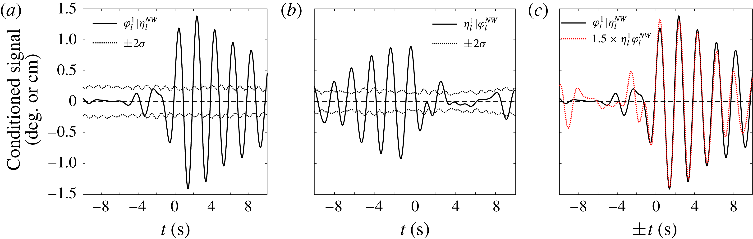
Conditioned signal analysis of the low pass roll (
 $\unicode[STIX]{x1D711}_{l}$
) and low pass waves (
 $\unicode[STIX]{x1D702}_{l}$
).
 $\unicode[STIX]{x1D70E}$
is the standard deviation used to estimate the confidence intervals. (a) Linear component of the low pass roll response conditioned on a NewWave-type form of the low pass waves. (b) Linear component of the low pass wave conditioned on a NewWave-type form of the low pass roll responses. (c) Reciprocity of the low pass wave (time reversed about
 $t=0$
and thus ‘
 $\pm t$
’ used here) and the low pass roll.

As in figure 18, but for the low pass roll (
 $\unicode[STIX]{x1D711}_{l}$
) and low pass sloshing (
 $\unicode[STIX]{x1D701}_{l}$
). The conditioned low pass roll signal has been mirrored in time about
 $t=0$
and multiplied by a numerical scaling factor of
 $0.75~\text{cm}~\text{deg}^{-1}$
.

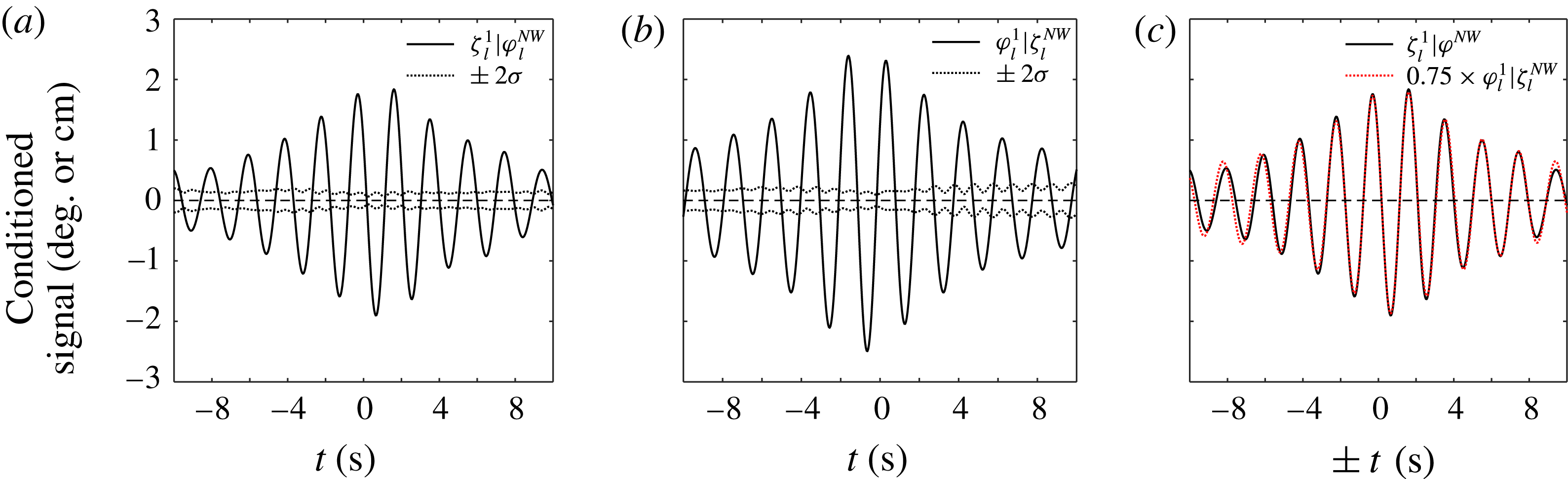
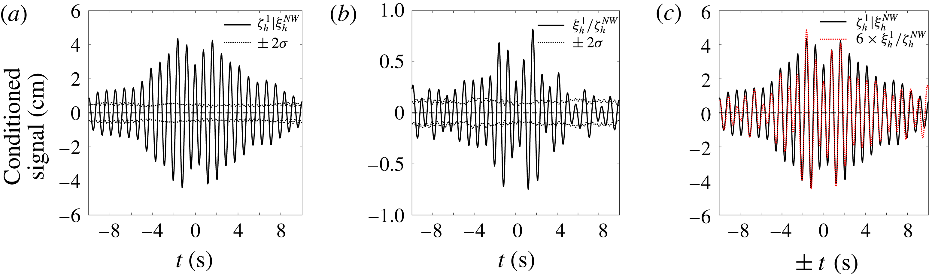
To test the theory above, the low pass roll signals conditioned on the low pass wave signals have been calculated. Phase-combination separation of the harmonics is employed, but as these data are frequency filtered, only the first harmonic is present. The first harmonic roll signal conditioned on the low pass wave signal is shown in figure 18(a), while figure 18(b) shows the linear component of the low pass waves conditioned on the low pass roll motions. The signal in figure 18(a) has a very similar shape to that in figure 18(b), with a reflection about
 $t=0$
. To provide a clearer illustration of this, these signals are plotted together in figure 18(c), where the conditioned low pass wave signals have been mirrored with respect to
 $t=0$
and amplified by a numerical scaling factor of
 $1.5\,^{\circ }~\text{cm}^{-1}$
, effectively
 $(\unicode[STIX]{x1D6FC}_{\unicode[STIX]{x1D702}}/\unicode[STIX]{x1D6FC}_{\unicode[STIX]{x1D711}})(\sum S_{\unicode[STIX]{x1D711}}/\sum S_{\unicode[STIX]{x1D702}})$
(see (6.5)). As observed, the two signals are very similar, confirming that the coupling between low pass waves and low pass roll motions is very close to linear, even with liquid in the partially filled tanks.
6.1.2 Coupling between low pass roll and low pass sloshing
As shown in figure 8, there is a response peak of the internal sloshing located at the same frequency as that of the main roll resonant response, which will be present in the low pass sloshing signal. The low pass roll may also couple to this low pass sloshing. To investigate this coupling, we apply the same process as in § 6.1.1, with results for low pass sloshing conditioned on roll and vice versa shown in figure 19, together with the indication of reciprocity. The very good agreement shown in figure 19(c) strongly supports the conclusion that the coupling between low pass roll and low pass sloshing is linear. It is worth noting that the sloshing signal measured from one (upwave) gauge is used for this type of analysis, but the results are unaffected by this choice.
6.1.3 Coupling between high pass incident waves and high pass roll
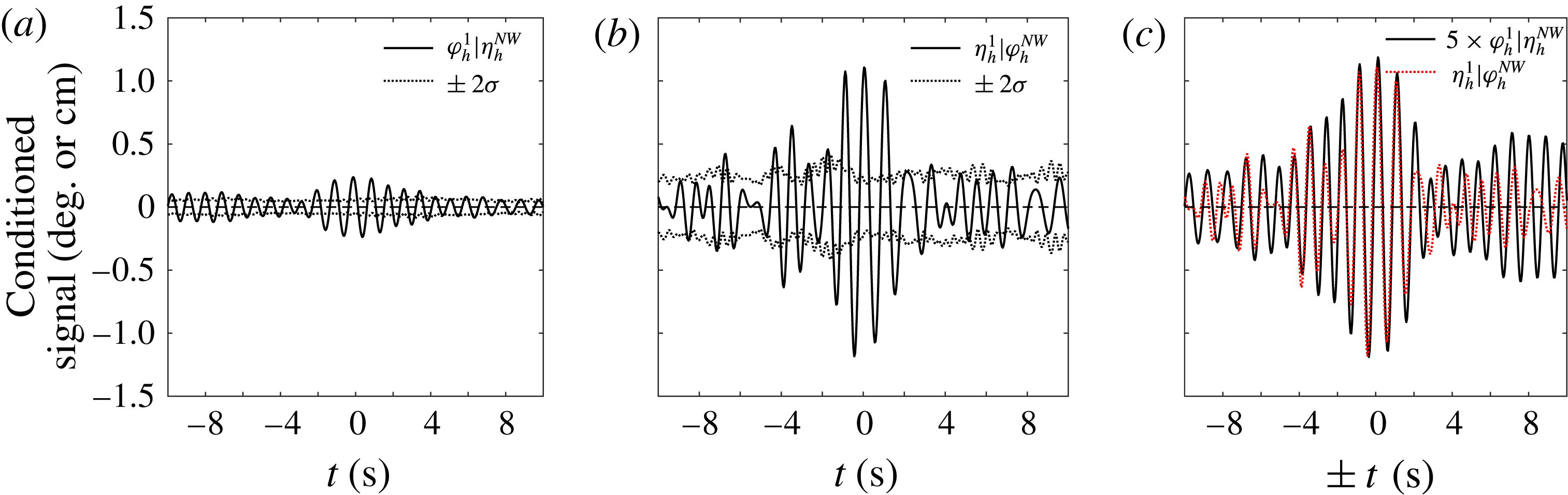
As the incident waves are very broadbanded, wave components at high frequency (the high pass waves) may drive roll motions linearly. To understand this coupling phenomenon, the same process as in § 6.1.1 is conducted for the high pass waves and high pass roll. Although we are now dealing with high pass signals where the higher harmonics are not filtered out, the results of the phase combination show no visible higher harmonics in the conditioned signals (so these are not shown), but significant linear components are observed. Figure 20 shows similar results as figure 18, but for the high pass waves and the high pass roll motions. In this case the scaling factor is
 $5~\text{cm}~\text{deg}^{-1}$
.
As in figure 18, but for the coupling between high pass waves (
 $\unicode[STIX]{x1D702}_{h}$
) and high pass roll (
 $\unicode[STIX]{x1D711}_{h}$
).

In the immediate vicinity of the conditioning point
 $t=0$
, the signal shapes shown in figure 20(c) are very similar, confirming that the coupling between the high pass roll signals and the high pass incident waves is a linear process. This suggests that some of the high pass roll must be driven linearly by the high pass waves. However, one can see that the overall agreement in figure 20(c) is reasonably good but not as good as in the previous examples. This is probably due to the fact that part of the high pass roll signal is a result of the higher harmonics of the main resonant roll response.
6.1.4 Coupling between high pass roll and high pass sloshing
The high pass roll may further couple to the internal sloshing. To investigate this coupling, reciprocity results for the high pass roll and the high pass sloshing signals (upwave gauge) are analysed in figure 21, analogous to the low pass results in figure 19.
As in figure 18, but for the coupling between high pass roll (
 $\unicode[STIX]{x1D711}_{h}$
) and high pass sloshing (
 $\unicode[STIX]{x1D701}_{h}$
).

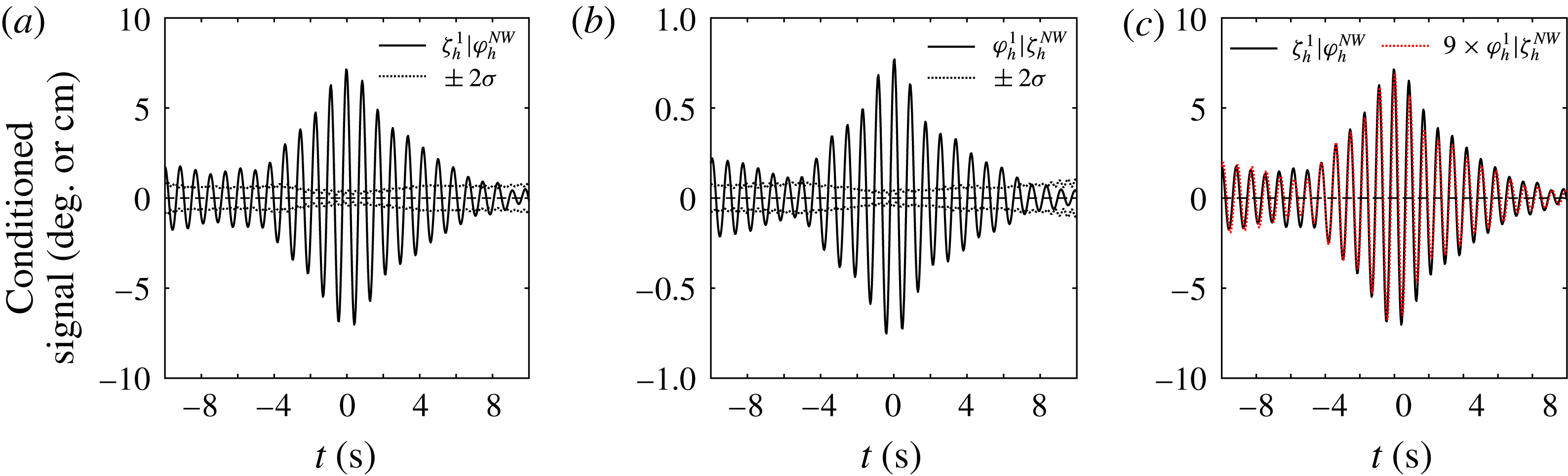
Again, only the first harmonic component of the conditioned signal is visible, and shown in figure 21, where the scaling coefficient in part (c) is 9 (
 $\text{cm}~\text{deg}^{-1}$
). The two signals are virtually identical, confirming that the coupling between high pass sloshing and high pass roll motions is a simple linear phenomenon.
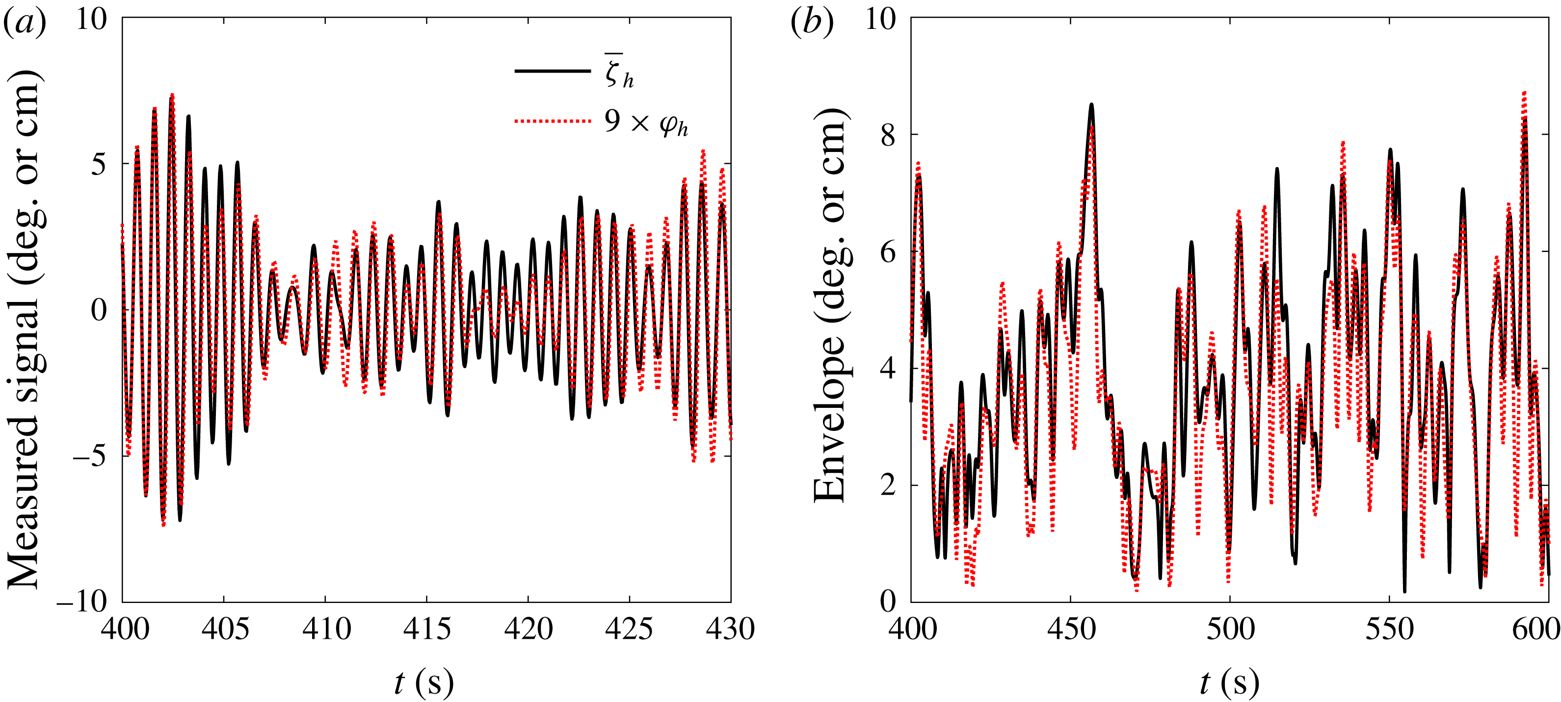
To further demonstrate the coupling between the internal sloshing and the high pass roll signals, representative time histories of the roll and sloshing signals (here the combination of two gauges, (upwave gauge – downwave gauge)/2) are plotted in figure 22(a), together with the high frequency roll signals scaled by 9 (
 $\text{cm}~\text{deg}^{-1}$
). Furthermore, their envelopes have been calculated using the Hilbert transform and plotted in figure 22(b). The envelopes show very similar trends for the high pass sloshing and the high pass roll signals, over a much larger time scale than in figure 22(a).
Comparison of the high pass sloshing signal (
 $\bar{\unicode[STIX]{x1D701}}_{h}$
= (upwave gauge – downwave gauge)/2) and the high pass roll signals (
 $\unicode[STIX]{x1D711}_{h}$
). (a) Time histories, (b) envelopes over a wider time window.

In addition to the coupling between high pass roll and sloshing, the coupling between high pass sway and sloshing is also investigated. Reciprocity results for high pass sway and high pass sloshing are given in figure 23, with the reasonable agreement seen and suggesting linear coupling between them. Given the linear coupling between the high pass roll and high pass sloshing shown in figure 21, one would expect the coupling between high pass sway and high pass roll should also be linear. This has been confirmed through reciprocity results, which are not shown here to avoid duplication.
As in figure 18, but for the coupling between high pass sloshing (
 $\unicode[STIX]{x1D701}_{h}$
) and high pass sway (
 $\unicode[STIX]{x1D709}_{h}$
).

As in figure 12, but for the high pass sloshing (
 $\unicode[STIX]{x1D701}_{h}$
) conditioned on the low pass roll (
 $\unicode[STIX]{x1D711}_{l}$
). (a) The second harmonics for conditioned high pass sloshing and high pass roll scaled by 9 (
 $\text{cm}~\text{deg}^{-1}$
). (b) The first, third and fourth harmonic components of the high pass sloshing conditioned on the low pass roll.

6.2 Identification of nonlinear coupling
As discussed earlier, the high pass roll may be driven linearly by the incident waves and/or nonlinearly through the roll higher harmonics. The coupling between the roll and sloshing signals (both for low pass and high pass signals) has been proved to be linear, so it is reasonable to expect nonlinear coupling between high pass sloshing and low pass roll.
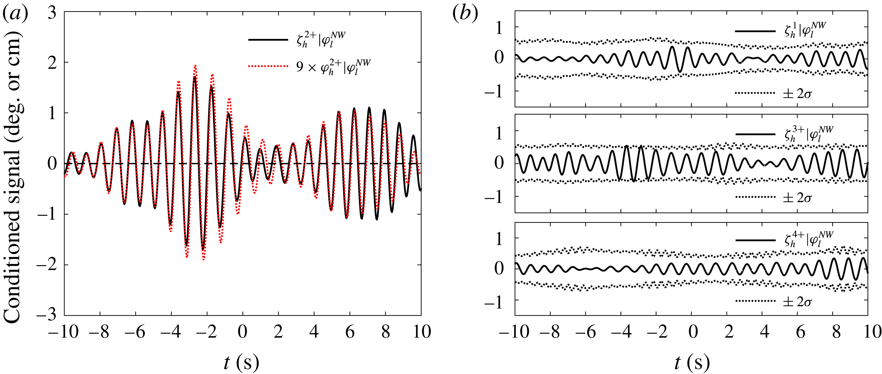
The first four harmonics of the high pass sloshing (again one gauge signal) conditioned on the low pass roll motions are shown in figure 24. The first, third and fourth harmonics are within the estimated 5 %–95 % error bars as shown in figure 24(b). In addition, the second harmonic of the high pass roll conditioned on the low pass roll motions amplified by a scaling coefficient of 9 (
 $\text{cm}~\text{deg}^{-1}$
) is plotted on top of the high pass conditioned sloshing signal in figure 24(a). These two signals are of very similar shape. This is due to the fact that high frequency roll and high frequency sloshing are linearly related. With this transfer coefficient, some slight differences between the two signals are visible in figure 24(a), so the level of match is not as good as that in figure 21(c). This difference is to be expected, because the procedure is based on a limited number of large profiles (top 30) picked out from a limited length of time history. The scaling coefficient used here is identical to that used in the high pass roll and high pass sloshing coupling. This indicates that no matter how the internal sloshing is driven, i.e. by higher harmonics of low pass roll motions (the main roll resonant signals) or by the high pass roll motions, the coupling between the subsequent roll motions and the internal sloshing is a linear process.
7 Conclusions
A series of experiments has been conducted in a deep water wave basin; these focused on the roll characteristics of a simple barge with partially filled spherical tanks as a model for an LNG carrier. This roll motion is a complex phenomenon and is of practical concern for side-by-side offloading operations. A signal processing approach based on combining an average shape of large events (NewWave) representation with a Stokes-type phase-combination method is used to study the large roll profiles with liquid cargo. The principal conclusions are as follows:
(i) We have observed and analysed a new form of coupling: low pass (linear) roll motion of a vessel driving sloshing at multiple (integer) frequencies of the low pass roll via nonlinear coupling. This induced sloshing itself back-reacts on the barge motion to drive high frequency roll (and sway) linearly.
(ii) In the physical experiments, high frequency roll is also driven by high frequency incident waves, but signal processing allows us to separate this simple effect out and to identify double frequency and triple frequency excitation of the sloshing mode.
(iii) We see no significant effect on roll from any other sloshing modes, instead various sources of excitation of the (1,1) sloshing mode – the lowest sloshing mode by frequency for spherical tanks. This suggests that considering only the (1,1) sloshing mode would be acceptable for the design or operation of LNG carriers with spherical tanks from the perspective of global motions during offloading operations.
(iv) Although the internal sloshing flow is significantly nonlinear, the coupling interaction from sloshing back to global roll motions of the model is demonstrated to be a simple linear feedback process (presumably through motion of the centre of gravity of the fluid in the tanks).
The analysis in this study can be regarded as the third of three recent papers using the NewWave-type methodology. In the first (Zhao et al. Reference Zhao, Wolgamot, Taylor and Eatock Taylor2017), we adopted NewWave-type wave groups (which are deterministic) with four different phases to excite gap resonances, and extracted higher harmonics in the gap resonance. The second (Zhao et al. Reference Zhao, Taylor, Wolgamot and Eatock Taylor2018) investigated the same problem but with broadbanded random incident waves, where NewWave-type wave profiles (similar to the groups in the first) were constructed through an averaging process. The present study introduced the idea of a conditioning process into the methodology used in part 2 (Zhao et al. Reference Zhao, Taylor, Wolgamot and Eatock Taylor2018), enabling the identification of linear and nonlinear coupling between random incident waves, roll motions and internal liquid cargo sloshing. The NewWave-type methodology is, for the first time, introduced to examine a substantially more complex set of random processes involving random external waves, body roll motion and internal free-surface sloshing, all coupled through both linear and weakly nonlinear interactions. In future work we aim to build a numerical model capturing these interactions between waves, roll and sloshing.
Acknowledgements
This work was funded by research and development grants from the University of Western Australia (UWA) and from Shanghai Jiao Tong University (SJTU). The first and third authors are grateful for support through the Shell EMI Offshore Engineering Initiative at UWA. The authors acknowledge useful discussions with Professor J. Yang at SJTU and Professor M. Efthymiou and Dr S. Draper at UWA. The authors would also like to thank the reviewers for their valuable comments which inspired us to delve further into the details of the sloshing modes, leading to the contents in appendix A.
Appendix A
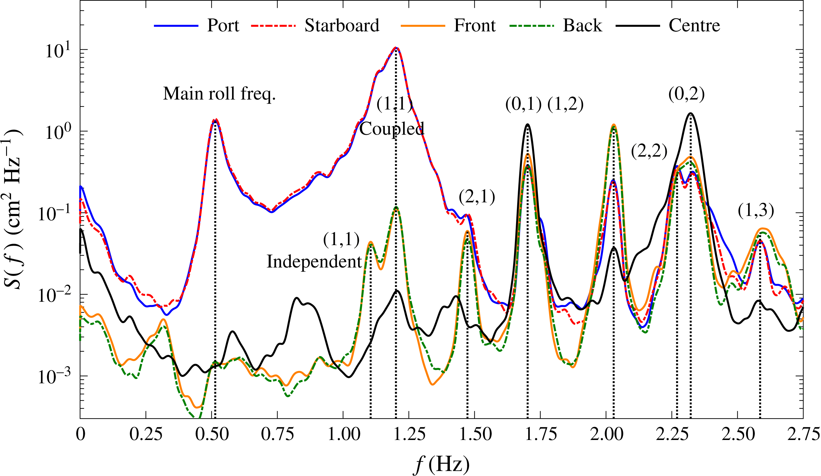
A series of sloshing modes in the spherical tanks at different load conditions are identified using all five wave probes inside the tanks in combination. Four of them are arc-shaped wave probes along the tank wall, while the remaining one is straight and goes through the geometric centre of the spherical tank, being vertical when the model is still. To demonstrate the different sloshing modes, the same results as in figure 8(c) are replotted by extending the horizontal axis up to 2.75 Hz and identifying the remaining sloshing modes from all the gauges, as shown in figure 25.
Power spectra of the measured sloshing signals with the model at the 50 % load condition under beam sea excitations, the vertical axes are on log scales. ‘Port’ refers to the arc-shape wave probe at the weather side, while ‘Back’, ‘Starboard’ and ‘Front’ located at intervals of 90
 $^{\circ }$
in anticlockwise direction. The ‘Centre’ wave probe is straight and goes through the geometric centre of the spherical tank.

All the experimentally determined frequencies of the sloshing modes (marked in figure 25) match the analytical approximations based on Faltinsen & Timokha (Reference Faltinsen and Timokha2009, Reference Faltinsen and Timokha2012) extremely well, apart from the (1,1) mode. We can see the ‘Port’ and ‘Starboard’ signals are dominated by a peak at 1.20 Hz, though there is a shoulder at 1.10 Hz which is the theoretical (1,1) mode value. In contrast, the ‘Front’ and ‘Back’ signals show each peak now much closer in magnitude at 1.10 Hz and 1.20 Hz (but significantly reduced in overall level). These very small (1,1) mode sloshing signals measured from the ‘Front’ and ‘Back’ wave probes in a beam sea excitation could be a result of swirling waves.
We see the same upshift phenomenon of the (1,1) mode frequency for all three load conditions, as shown in table 2. It is very likely to be a result of the interaction between the global roll motions and the (1,1) mode sloshing. This can be explained in terms of the resonant modes of a 2 degrees-of-freedom (DOF) system, where the two are the global roll motions and the (1,1) mode sloshing.
Taking an undamped 2-DOF system as an example, e.g. fixed point – spring (
 $k_{1}$
) – mass (
 $m_{1}$
) – spring (
 $k_{2}$
) – mass (
 $m_{2}$
), we have the differential equations of motion
 $m_{1}\ddot{x}_{1}+(k_{1}+k_{2})x_{1}-k_{2}x_{2}=0$
and
 $m_{2}\ddot{x}_{2}-k_{2}x_{1}+k_{2}x_{2}=0$
, where
 $x_{1}$
and
 $x_{2}$
are the displacements of the two masses. Solving this coupled system for inline vibration shows that the frequency of the lower mode is downshifted from
 $\sqrt{k_{1}/m_{1}}$
by the addition of the second mode, whereas the frequency of the higher mode is upshifted from
 $\sqrt{k_{2}/m_{2}}$
, these being the resonant frequencies for the elements in isolation.
None of the other sloshing modal frequencies are significantly shifted because their mode shapes do not include any (much) horizontal motion of the centre of mass of the tank liquid, and thus there is no significant coupling with global roll motions.
Appendix B
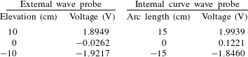
Calibrations of the instruments including external resistance-type wave probes, internal curved wave probes and the load cells on the mooring lines (not reported in this paper) were carried out prior to the model tests.
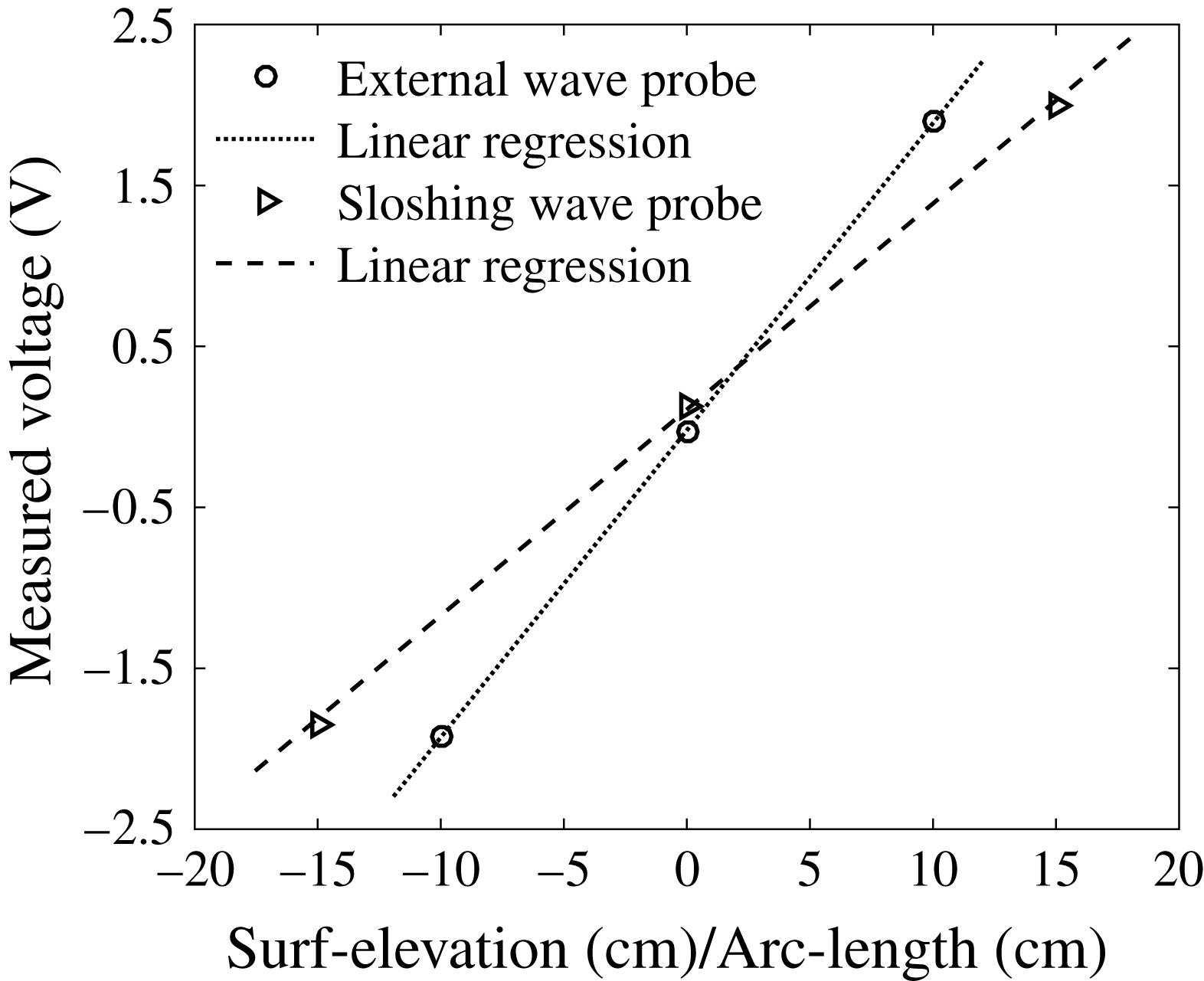
Some representative calibration results are listed in table 3. The corresponding calibration results are also plotted in figure 26. It can be seen that the instruments show very good linearity.
Calibration results of the instrumentations.

Representative calibration results of the instrumentations.

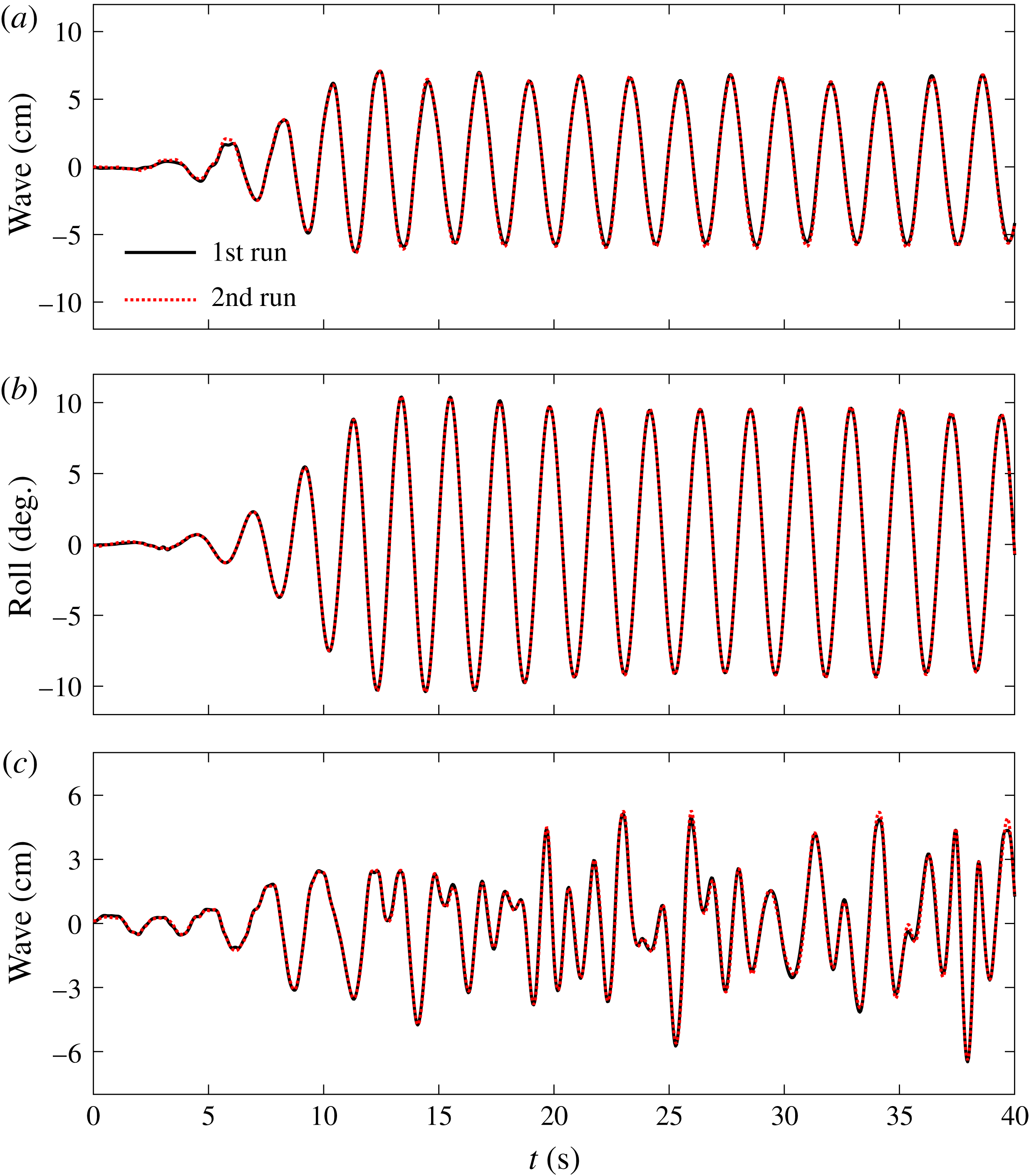
The repeatability of the wave generation and motion measurements is shown in figure 27, with (a) showing the free-surface elevations measured at a certain distance away from the side end of the vessel (so the disturbed wave field) and (b) the roll motions of the model. The experimental set-up in (a,b) is the same as in figure 2, except that the model has a natural frequency of 0.46 Hz with frozen cargo. The regular wave test results suggest that the vessel motions and the diffracted wave fields (with the model in place) show extremely good repeatability for both the starting transient and the steady-state behaviour.
Repeatability of the wave generations and vessel motions, (a) free-surface elevations in regular wave tests, (b) roll motions of the vessel with frozen cargo in regular wave tests, (c) diffracted wave fields in white noise wave tests. Note the diffracted wave fields in (c) were measured in a previous test conducted in the same wave basin but for two fixed boxes (Zhao et al. Reference Zhao, Wolgamot, Taylor and Eatock Taylor2017) under similar white noise waves.

In this study, we have focused on white noise waves, which we believe have the same repeatability, and thus we did not repeat these in this experiment. However, we provide some indirect evidence to demonstrate the repeatability of white noise irregular wave generation in figure 27(c), which shows waves measured in the same wave basin using the same wave gauge. These white noise waves, with a slightly larger significant wave height than used in the present study, were generated for the gap resonance problems (Zhao et al. Reference Zhao, Wolgamot, Taylor and Eatock Taylor2017) where two identical boxes are fixed together in side-by-side configuration, forming a narrow gap. In the experiment of Zhao et al. (Reference Zhao, Wolgamot, Taylor and Eatock Taylor2017), the white noise waves were generated twice with the two fixed boxes in place, but the bilge geometry of the boxes was changed from round (for the 1st run) to square (for the 2nd run) shape. The free-surface elevations were recorded 5.04 m away from the side end of the fixed boxes, where the gap resonance effects due to different geometries are thought to be small. As confirmed in figure 27(c), at the beginning, the two diffracted white noise wave signals match very well, and slight discrepancies appear later on which are believed to be a result of the slightly different gap resonances generated by different box geometries.
Given the good agreement shown in figure 27, we believe we have provided sufficient evidence for the repeatability of the wave generation process and vessel motion measurements, both for regular and irregular waves.