


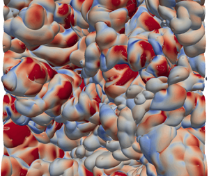

1. Introduction
In free-shear flows (e.g. jets, wakes and mixing layers), the turbulent regions and the non-turbulent regions are separated by continuous, thin and highly contorted interfacial layers, which is also known as turbulent/non-turbulent interface (TNTI; see da Silva et al. (Reference da Silva, Hunt, Eames and Westerweel2014) and references therein). The physical properties of the TNTI govern the exchange of mass and momentum between the turbulent and non-turbulent regions and, consequently, a thorough understanding of the TNTI is of critical importance to model the growth of free-shear turbulence and the accompanying scalar mixing.
The pioneering work of Corrsin & Kistler (Reference Corrsin and Kistler1955) pointed out that there exists a viscous superlayer at the outer edge of the TNTI and the thickness of the viscous superlayer is comparable to the Kolmogorov length-scale. This assumption made by Corrsin & Kistler (Reference Corrsin and Kistler1955) was first confirmed by Taveira & da Silva (Reference Taveira and da Silva2014). The continuous viscous superlayer is characterised by the overwhelming dominance of pure shear motions without solid-body rotation (Xie et al. Reference Xie, Yin, Zhang and Zhou2023; Yin et al. Reference Yin, Xie, Zhang and Zhou2023). The characteristic features of the TNTI and the entrainment process through which the non-turbulent fluid points at the vicinity of the TNTI become turbulent have been explored extensively for more than half a century (see, for example, Westerweel et al. Reference Westerweel, Fukushima, Pedersen and Hunt2009; Holzner & Lüthi Reference Holzner and Lüthi2011; Taveira & da Silva Reference Taveira and da Silva2013; da Silva, Lopes & Raman Reference da Silva, Lopes and Raman2015; Xu, Long & Wang Reference Xu, Long and Wang2023). It is commonly believed that there are two different mechanisms contribute to the entrainment process: small-scale nibbling and large-scale engulfment and the entrainment process is dominated by the effect of small-scale nibbling (Holzner & Lüthi Reference Holzner and Lüthi2011; da Silva et al. Reference da Silva, Hunt, Eames and Westerweel2014). Until now, understanding of the turbulent entrainment remains challenging. As a matter of fact, in a quite recent work by van Reeuwijk, Vassilicos & Craske (Reference van Reeuwijk, Vassilicos and Craske2021), it is suggested that ‘understanding of turbulent entrainment (the transport of fluid from regions of relatively low to relatively high levels of turbulence) remains fragmented’. One of the challenges is related to the fact that the local entrainment velocity  $v_n$ is thought to be comparable to the Kolmogorov velocity (Holzner & Lüthi Reference Holzner and Lüthi2011), and the TNTI can be strongly contorted with fractal-like geometry covering a wide range of length scales (de Silva et al. Reference de Silva, Philip, Chauhan, Meneveau and Marusic2013).
The growth rate of free shear turbulent flows is directly determined by the local entrainment velocity and the corresponding instantaneous contorted surface area. It is worth mentioning that albeit the entrainment process across the TNTI has been studied extensively both experimentally and numerically, only a few studies (Holzner & Lüthi Reference Holzner and Lüthi2011; Jahanbakhshi & Madnia Reference Jahanbakhshi and Madnia2016) have strictly checked the balance between the integral volume flux, i.e. integrating the local entrainment velocity  $v_n(t)$ over the highly contorted area of the TNTI,
 $Q(t)=\int v_n(t)\, {\rm d} A(t)$ and the global volume flux
 $Q_0(t)=-{\rm d} V_J(t)/{\rm d} t$. The global volume flux can also be given by
 $Q_0(t)=u_eA_0$ with
 $u_e$ being the mean entrainment velocity and
 $A_0$ being the projected area of the TNTI (Sreenivasan, Ramshankar & Meneveau Reference Sreenivasan, Ramshankar and Meneveau1989). Recently, an alternative but probably less-direct way to model the turbulent entrainment process across the TNTI is proposed by Zhou & Vassilicos (Reference Zhou and Vassilicos2017) and Er, Laval & Vassilicos (Reference Er, Laval and Vassilicos2023). The Corrsin length
 $\eta _I \sim \nu /\langle v_n \rangle$, which is based on the mean entrainment velocity and the thickness of the TNTI, and the fractal property of the TNTI are involved for an indirect estimation of the surface area (Zhou & Vassilicos Reference Zhou and Vassilicos2017; Er et al. Reference Er, Laval and Vassilicos2023). The Corrsin length and the fractal property are expected to only be accurately observed at high Reynolds numbers, albeit the recent work by Zhou & Vassilicos (Reference Zhou and Vassilicos2017) and Er et al. (Reference Er, Laval and Vassilicos2023) suggested that one could predict the scaling of the mean entrainment velocity based on the characteristics of the Corrsin length and the fractal property even at moderate Reynolds numbers.
Another aspect, perhaps equally significant but less noticed is that for self-similar/self-preserving turbulent shear flow the entrainment process across the TNTI is closely related to the newly reported non-equilibrium dissipation law (Vassilicos Reference Vassilicos2015; Zhou & Vassilicos Reference Zhou and Vassilicos2017). The dissipation assumption, which is also referred to as the zeroth law of turbulence (Benzi & Toschi Reference Benzi and Toschi2023), is normally required to derive the growth law of free shear flows. Different dissipation assumptions (i.e. equilibrium dissipation law and non-equilibrium dissipation law) can normally lead to distinctly different growth behaviour of turbulent shear flows (Nedić, Vassilicos & Ganapathisubramani Reference Nedić, Vassilicos and Ganapathisubramani2013; Dairay, Obligado & Vassilicos Reference Dairay, Obligado and Vassilicos2015; Cafiero & Vassilicos Reference Cafiero and Vassilicos2020). It is worth mentioning that aside from classical self-similar analysis (Townsend Reference Townsend1956, Reference Townsend1976), there are other methods to derive the scaling law of shear flows (see, for example, George Reference George1989; Sadeghi, Oberlack & Gauding Reference Sadeghi, Oberlack and Gauding2018). Furthermore, based on the variation of the TNTI surface area in a self-similar period, the mean entrainment velocity can also be derived from the scaling law, as shown below, which can provide a simple law of entrainment velocity and has not been done in previous studies.
The temporal evolution equation of a non-material infinitesimal element of area  $\delta A$, derived by Phillips (Reference Phillips1972), has been widely used to investigate the production and destruction mechanisms of the turbulent flame surface area (Candel & Poinsot Reference Candel and Poinsot1990; Trouvé & Poinsot Reference Trouvé and Poinsot1994; Echekki & Chen Reference Echekki and Chen1999), which is also applicable to the evolution of the TNTI surface area. The growth of the TNTI area strongly depends on the turbulent entrainment process and the surface curvature (Phillips Reference Phillips1972). However, a few studies have directly analysed the evolution of the three-dimensional (3-D) TNTI surface area and combined it with the surface curvature. Recently, Neamtu-Halic et al. (Reference Neamtu-Halic, Krug, Mollicone, van Reeuwijk, Haller and Holzner2020) studied the effect of nearby coherent structures on the evolution of the two-dimensional (2-D) TNTI surface area, but the comprehensive understanding of the coupling between the production and destruction of the TNTI surface area, surface curvature and the entrainment process remains elusive. Furthermore, the Reynolds number (the inflow Reynolds number
 $R{e_0} = {{u{h_0}} / \nu } = 3700$) used in the work of Neamtu-Halic et al. (Reference Neamtu-Halic, Krug, Mollicone, van Reeuwijk, Haller and Holzner2020) is relatively low to draw conclusions about the evolution characteristics of the TNTI at high Reynolds numbers. It is well-known that chemical reactions often occur near the TNTI in non-premixed flames (Cleary & Klimenko Reference Cleary and Klimenko2009; Gampert et al. Reference Gampert, Kleinheinz, Peters and Pitsch2014) and the TNTI governs the mixing rates between different species (da Silva et al. Reference da Silva, Hunt, Eames and Westerweel2014). Thus, fully understanding the evolution of the TNTI surface area is related to the modelling of the scalar dissipation rate (or some other related quantity) in numerical simulations of reacting flows and is an important research topic.
In this paper, a temporally evolving turbulent plane jet is numerically investigated by means of direct numerical simulation (DNS). The numerical data of a temporally shear flow allow a quantitative assessment of the turbulent entrainment across the TNTI. The remaining parts of the paper are organised as follows. In § 2, we present the DNS details along with the validation of the numerical data. A theoretical analysis of the mean flow scaling law based on the computational results of the TNTI area is presented in § 3. In § 4, we further explore the physical mechanisms responsible for the production/destruction of the TNTI area. Finally, our main findings are summarised in § 5.
2. DNS of a temporally evolving turbulent plane jet
The DNS data with a high spatial resolution are the essential prerequisites for an accurate evaluation of the local turbulence characteristics near the TNTI along with the corresponding entrainment process. An open-source high-fidelity parallel solver ‘Incompact3d’ (Laizet & Lamballais Reference Laizet and Lamballais2009; Laizet, Lamballais & Vassilicos Reference Laizet, Lamballais and Vassilicos2010; Laizet & Li Reference Laizet and Li2011) with spectral-like resolution (Lele Reference Lele1992) is used for the DNS of the temporally evolving turbulent plane jet with a moderate Reynolds number.
2.1. Numerical details
Following previous numerical studies (da Silva & Métais Reference da Silva and Métais2002; Hayashi, Watanabe & Nagata Reference Hayashi, Watanabe and Nagata2021), a hyperbolic-tangent function is employed to describe the vertical distribution of the initial mean streamwise velocity  $U_{in}(Y)$, i.e.
 \begin{equation} U_{in}(Y)=\frac{U_J}{2}+\frac{U_J}{2} \tanh \left[\frac{H_J}{4 \theta_0}\left(1-\frac{2\lvert Y \rvert}{H_J}\right)\right],\end{equation}
where  $U_J=1$ and
 $\theta _0/H_J=35$ with
 $\theta _0$ and
 $H_J$ being the initial momentum thickness and the width of the nozzle, respectively. The mean initial velocity in the two other directions is set to zero, i.e.
 $V_{in}(Y)= 0$ and
 $W_{in}(Y)= 0$. Throughout the paper, unless otherwise defined, the values of the mean velocity components and the corresponding fluctuating components are presented by uppercase and lowercase letters, respectively. The periodic boundary conditions are adopted in the two quasi-homogeneous directions (i.e.
 $X$ and
 $Z$ directions), whereas the free slip boundary condition is used in the vertical direction.
For an efficient transition to the self-similar/self-preserving state, artificially generated 3-D disturbances are superimposed onto the initial mean velocity field ( $U_{in}$,
 $V_{in}$,
 $W_{in}$) within the vertical range
 $-1/2 \le Y/H_J \le 1/2$. The generation of the initial disturbances is based on the diffusion procedure proposed by Kempf, Klein & Janicka (Reference Kempf, Klein and Janicka2005). Relatively small-amplitude disturbances (i.e. the root-mean-square (r.m.s.) values of the velocity fluctuations in three directions are only
 $0.02 U_J$) be superposed onto the initial mean velocity field to allow a natural outward growth of the turbulent plane jet.
The computational details and the corresponding geometric parameters are listed in table 1. Here, the initial Reynolds number  $Re_{J}=U_JH_J/\nu$, where
 $\nu$ is the kinematic viscosity, is set to 4000. This moderate Reynolds number is chosen to ensure a sufficiently fine spatial resolution and, consequently, accurately capture the instantaneous TNTI along with the nearby turbulent flow dynamics. For instance, the first-order and second-order derivatives of vorticity are required to compute the local turbulent entrainment (Holzner & Lüthi Reference Holzner and Lüthi2011). The lengths
 $L_X$,
 $L_Y$ and
 $L_Z$ denote the sizes of the computational domain along the streamwise, vertical and spanwise directions, respectively. Hereafter,
 $X$,
 $Y$ and
 $Z$ refer to the streamwise, vertical and spanwise directions, respectively. The size of the simulation domain is
 $L_X \times L_Y \times L_Z = 8 H_J \times 12 H_J \times 8 H_J$ and a total number of
 $N_X \times N_Y \times N_Z = 768 \times 1025 \times 768$ grid mesh points are used for the spatial discretisation. With respect to the finite-difference discretisation, a sixth-order central compact scheme with spectral-like resolution (Lele Reference Lele1992) is employed. A third-order Adams–Bashforth scheme is adopted for time advancement with
 $\Delta t / (H_{J}/U_{J})=0.0015$. It is worth mentioning that the size of the simulation domain and the corresponding mesh number are comparable to or even better than those used in Hayashi et al. (Reference Hayashi, Watanabe and Nagata2021). To avoid the normal boundary conditions affecting the evolution of the turbulent region, we carefully selected the box size along the normal direction, i.e.
 $L_Y=12H$. This box size is larger than the normal length used in previous studies (Watanabe et al. Reference Watanabe, da Silva, Nagata and Sakai2017; Silva, Zecchetto & da Silva Reference Silva, Zecchetto and da Silva2018; Hayashi et al. Reference Hayashi, Watanabe and Nagata2021) and is nearly twice that used by Silva et al. (Reference Silva, Zecchetto and da Silva2018). Further validation of the choice of the streamwise and spanwise simulation domains is confirmed by performing an additional DNS with a larger simulation domain, i.e.
 $L_X \times L_Y \times L_Z = 16 H_J \times 12 H_J \times 16 H_J$ and the corresponding number of grids is
 $N_X \times N_Y \times N_Z = 1536 \times 1025 \times 1536$ (
 $\simeq 2.4 \times {10^{ 9}}$). The numeral treatment of the additional DNS is the same as that with a small domain.
Computational and geometric details.

2.2. Simulation validation and spatial resolution
Figure 1 shows the vertical distributions of the normalised one-point statistics (i.e. the mean streamwise velocity  $U$ and r.m.s. velocities
 $U_{rms}$,
 $V_{rms}$ and
 $W_{rms}$) at two different time steps (
 $T/T_{ref}=25.5$ and 36.0, where
 $T_{ref}=H_J/U_J)$. The corresponding results from previous numerical (i.e. da Silva & Métais Reference da Silva and Métais2002; da Silva & Pereira Reference da Silva and Pereira2008; Watanabe et al. Reference Watanabe, Sakai, Nagata, Ito and Hayase2014b; Hayashi et al. Reference Hayashi, Watanabe and Nagata2021) and experimental (i.e. Gutmark & Wygnanski Reference Gutmark and Wygnanski1976; Thomas & Prakash Reference Thomas and Prakash1991; Stanley, Sarkar & Mellado Reference Stanley, Sarkar and Mellado2002) investigations are included for comparison. It can be seen that our simulation results are in reasonably good accord with those in previous studies. Here,
 $U_C$ and
 $b_U$ denote the centreline mean velocity and the jet half-width, respectively. Hereafter, the subscript
 $C$ denotes a variable along the centreline and the half-width
 $b_U$ is defined as the vertical distance between the jet centreline and the location where
 $U(Y)/{U_C} = 0.5$.
The distributions of the normalised mean flow velocity and r.m.s. velocities. For comparison, results from previous investigations (i.e. Gutmark & Wygnanski Reference Gutmark and Wygnanski1976; Thomas & Prakash Reference Thomas and Prakash1991; da Silva & Métais Reference da Silva and Métais2002; Stanley et al. Reference Stanley, Sarkar and Mellado2002; da Silva & Pereira Reference da Silva and Pereira2008; Watanabe et al. Reference Watanabe, Sakai, Nagata, Ito and Hayase2014b; Hayashi et al. Reference Hayashi, Watanabe and Nagata2021) are included.

To capture small-scale flow dynamics across the TNTI and the small-scale local entrainment velocity  $v_n$, high-order derivatives (e.g. the first-order and second-order derivatives of the vorticity) need to be accurately solved. In this study, a high-order compact scheme is adopted, and the global Reynolds number is set to be moderately low. The current spatial resolution follows the suggestion by Laizet, Nedić & Vassilicos (Reference Laizet, Nedić and Vassilicos2015) that a spatial resolution less than
 $2\eta$ is necessary to have a correct reproduction of the strain-rate and rotation tensors when using the solver Incompact3d. As shown in figure 2(a), the normalised spatial resolution
 $(\Delta X \Delta Y \Delta Z)^{1/3}/\eta$ is always below 1.2, with
 $\Delta X$,
 $\Delta Y$ and
 $\Delta Z$ being the mesh sizes in the streamwise, vertical and spanwise directions, respectively, and
 $\eta$ is the Kolmogorov scale. Figure 2(b) shows that the spatial resolution
 $(\Delta X \Delta Y \Delta Z)^{1/3}/\eta$ at the TNTI detected by a wider range of vorticity magnitude (
 $1.0\times {10^{-5}}\le {\vert \boldsymbol \omega \vert }_{th} / {\vert \boldsymbol \omega \vert }_{max} \le 1.0\times {10^{-3}}$) is mostly smaller than 1.0 and the peaks of the probability distribution function (PDF) profiles are found around
 $(\Delta X \Delta Y \Delta Z)^{1/3}/\eta \simeq 0.45$. Further validation of the current spatial resolution is done by assessing the balance between the integral volume flux and the global volume flux, as will be demonstrated below.
(a) Vertical distributions of the normalised spatial resolution  $(\Delta X \Delta Y \Delta Z)^{1/3}/\eta$ at
 $T/T_{ref}=25.5$ and (b) the PDF distribution of the local resolution at the TNTI for three different thresholds
 ${\vert \boldsymbol \omega \vert }_{th} / {\vert \boldsymbol \omega \vert }_{max} = 1.0\times {10^{-5}}$ (red solid line),
 $1.6\times {10^{-4}}$ (cyan solid line) and
 $1.0\times {10^{-3}}$ (green solid line) with
 ${\vert \boldsymbol \omega \vert }_{max}$ being the maximum vorticity magnitude.

2.3. Evaluation of the self-similarity property
Figure 1(a) suggests that the vertical distribution of mean velocity is self-similar/self-preserving. To further evaluate the self-similar behaviour of the mean flow, the jet shape factor  $F(t)$ (Hickey, Hussain & Wu Reference Hickey, Hussain and Wu2013) is computed (see figure 3). The jet shape factor
 $F(t)$ is the ratio of the displacement thickness
 $\delta _{J}=\int U(Y)/U_C \,{\rm d} Y$ to the momentum thickness
 $\theta _{J}=\int U(Y)^2/U_C^2 \,{\rm d} Y$, that is
 $F(t) = \delta _{J}(t) / \theta _{J}(t)$. The time evolution of
 $\delta _{J}$ and
 $\theta _{J}$ are also included in figure 3. The jet shape factor
 $F$ remains nearly constant, i.e.
 $F \simeq 1.37$ after
 $T/T_{ref}=10.0$.
Time evolution of the shape factor  $F(t)$, the displacement thickness
 $\delta _{J}(t)$ and the momentum thickness
 $\theta _{J}(t)$. The horizontal line indicates
 $F \simeq 1.37$.

The self-similar behaviour of the mean velocity and the corresponding constant jet shape factor  $F$ have been confirmed in the previous discussion. The self-similar/self-preserving state can be further evaluated by the second-order statistics such as r.m.s. velocity (Almagro, García-Villalba & Flores Reference Almagro, García-Villalba and Flores2017). Figure 4 shows the vertical distributions of the normalised r.m.s. velocity components and the Reynolds stress as a function of
 $Y/b_U$. It can be seen that although the profiles are not smooth and exhibit oscillations to some extent, which is probably related to the insufficient data samples for a given time step, a reasonably good profile can still be obtained. A quantitative assessment of self-similarity is determined by calculating the area enclosed within the normalised profiles. Take, for instance, the integral function
 $S_{\boldsymbol {u}}$ for the normalised profiles of
 ${\boldsymbol {u}}_{rms}$ is defined by
 $S_{\boldsymbol {u}} = \int {{{\boldsymbol {u}}_{rms}} \,{\rm d}Y/{\boldsymbol {u}}_{rms}^{max}{b_U}}$. It is evident from figure 5 that the profiles evaluating the self-similar states become roughly constant for
 $T/T_{ref} >20.0$. The corresponding turbulent Reynolds number
 $Re_{\lambda }$ based on the Taylor microscale
 $\lambda$ remains nearly constant at approximately
 $Re_{\lambda } = {u_{rms}}\lambda /\upsilon \simeq 58.8$ for
 $T/T_{ref} >20.0$.
Vertical distributions of the normalised (a)  $U_{rms}$, (b)
 $V_{rms}$ (c)
 $W_{rms}$ and
 $\langle u'v' \rangle$ at different time steps, normalised by the peak values of the respective curves.

Time evolution of the integrals, i.e.  $S_{u}(t)$,
 $S_{v}(t)$,
 $S_{w}(t)$ and
 $S_{uv}(t)$.

3. Surface area of the TNTI and the scaling law of the mean flow
The entrainment processes of free shear flows are closely related to turbulent flow dynamics near the TNTI. We first explore the identification of the TNTI and temporal evolution of the TNTI surface area, and also establish the relationship of the turbulent entrainment process and the TNTI surface area, which enables us to derive the scaling law of the mean flow.
3.1. Identification and surface area of the TNTI
Figure 6 shows the contours of the magnitude of the vorticity field  $\vert \boldsymbol \omega \vert$ in a randomly chosen 2-D
 $X\unicode{x2013}Y$ plane at
 $T/T_{ref}=19.5$ and the isocontour lines corresponding to three different vorticity magnitudes (represented by solid lines) are also included. Here,
 ${\boldsymbol {\omega }}$ stands for the vorticity vector with
 $\omega _i=\varepsilon _{i j k} \partial u_k / \partial x_j$, where the subscripts
 $i = 1$,
 $2$ and
 $3$ represent
 $X$,
 $Y$ and
 $Z$ directions, respectively. Throughout this paper, the bold letters indicate vectors, and the symbol ‘
 $|\ |$’ represents the magnitude of a vector. The symbol
 $\boldsymbol \omega _{max}$ denotes the maximum magnitude of vorticity within the turbulent region for a particular time step. Based on the interface orientation relative to the mean streamwise velocity, the TNTI can generally be classified into three different types as conducted by Watanabe et al. (Reference Watanabe, Sakai, Nagata, Ito and Hayase2014b): leading edge (oriented towards the streamwise velocity), trailing edge (oriented opposite to the streamwise direction) and cross-streamwise edge (aligned with the mean flow or, equivalently, perpendicular to the cross-stream
 $Y\unicode{x2013}Z$ plane), as shown in figure 6.
The logarithmic contours of the magnitude of vorticity at  $T/T_{ref}=19.5$. The three solid lines correspond to
 ${\vert \boldsymbol \omega \vert }_{th}(t) / {\vert \boldsymbol \omega \vert }_{max}(t)= 1.0 \times {10^{ - 5}}$ (white one),
 $1.6 \times {10^{ - 4}}$ (black one) and
 $1.0 \times {10^{ - 3}}$ (blue one), respectively. Only part of the simulation domain is plotted.

As can be seen from figure 6, for a wide range of vorticity magnitudes  $1.0\times {10^{-5}}\le {\vert \boldsymbol \omega \vert }_{th}(t) / {\vert \boldsymbol \omega \vert }_{max}(t) \le 1.0\times {10^{-3}}$, the turbulent regions surrounded by TNTI rarely change as it should be. Following the previous study by Zhou & Vassilicos (Reference Zhou and Vassilicos2017), the vorticity norm, which is based on the maximum vorticity magnitude
 $\vert \boldsymbol \omega \vert _{max}(t)$, is used to identify the TNTI. The dependence of the volume fraction on the threshold value and the derivative of the volume fraction with respect to the threshold are plotted in figure 7. A distinct plateau where
 $-{\rm{d}}{V_T}/{\rm{dlog}}_{10}({\vert \boldsymbol{\omega} \vert _{th}}) \simeq 0$ within the range
 $1.0\times {10^{-7}} \le {\vert \boldsymbol \omega \vert }_{th}(t) / {\vert \boldsymbol \omega \vert }_{max}(t) \le 1.0\times {10^{-3}}$ can be readily identified. In order to accurately identify the TNTI, it is crucial to carefully choose an appropriate vorticity threshold. Based on the joint probability density distribution of the normalised vorticity magnitude
 ${\vert \boldsymbol \omega \vert }_{th} / {\vert \boldsymbol \omega \vert }_{max}$ and vertical height
 $Y/b_U$ (not shown herein), we also confirm that the presence of numerical noise (Zhang, Watanabe & Nagata Reference Zhang, Watanabe and Nagata2018) within the range
 $1.0\times {10^{-7}} \le {\vert \boldsymbol \omega \vert }_{th}(t) / {\vert \boldsymbol \omega \vert }_{max}(t) \le 1.0\times {10^{-5}}$, despite the turbulence volume hardly changes with the threshold
 ${\vert \boldsymbol \omega \vert }_{th} / {\boldsymbol \omega }_{max}$. Therefore, any threshold selection within the range
 $1.0\times {10^{-5}} \le {\vert \boldsymbol \omega \vert }_{th}(t) / {\vert \boldsymbol \omega \vert }_{max}(t) \le 1.0\times {10^{-3}}$ can be employed to detect TNTI and similar results can be obtained. Hereafter, the threshold
 ${\vert \boldsymbol \omega \vert }_{th}(t) / {\vert \boldsymbol \omega \vert }_{max}(t) = 1.6 \times {10^{ - 4}}$ corresponding to the black line in figure 6 is adopted for the identification of the TNTI.
(a) The volume fraction of the turbulent region with  $\vert \boldsymbol \omega \vert \ge {\vert \boldsymbol \omega \vert }_{th}$ as a function of the threshold
 ${\vert \boldsymbol \omega \vert }_{th} / {\vert \boldsymbol \omega \vert }_{max}$ and (b) the derivative of the volume fraction with respect to the threshold. The vertical dashed line indicates
 ${\vert \boldsymbol \omega \vert }_{th}(t) / {\vert \boldsymbol \omega \vert }_{max}(t)= 1.6 \times {10^{-4}}$ and the shadowed areas correspond to the range
 $1.0\times {10^{-5}}\le {\vert \boldsymbol \omega \vert }_{th}(t) / {\vert \boldsymbol \omega \vert }_{max}(t) \le 1.0\times {10^{-3}}$.

The method introduced by Yurtoglu, Carton & Storti (Reference Yurtoglu, Carton and Storti2018), which employs a grid-based approach for computing implicitly defined surface integrals, is adopted to compute the surface area  $A(t)$ and the integral volume flux
 $Q(t) = \int {{v_n}(t)} \,{\rm d}A(t)$, where
 ${v_n(t)}$ denotes the local entrainment velocity closely associated with the development of the plane jet. The method uses the divergence theorem along with the characteristics of surface normal vectors to transform the surface integral into a volume integral, i.e.
 \begin{equation} Q(t) = \int {{v_n}(t)} \,{\rm d}A(t) ={-}\sum_{I, J, K} (v_n)_{I, J, K} {\frac{\boldsymbol{\nabla} \boldsymbol{\chi}(|{\boldsymbol{\omega}} |)_{I, J, K} \boldsymbol{\cdot} \boldsymbol{\nabla} |{\boldsymbol{\omega}} |_{I, J, K}}{\sqrt{\boldsymbol{\nabla} |{\boldsymbol{\omega}} |_{I, J, K} \boldsymbol{\cdot} \boldsymbol{\nabla} |{\boldsymbol{\omega}} |_{I, J, K}}}} \Delta X \Delta Y \Delta Z, \end{equation}
where
 \begin{equation} \boldsymbol{\chi} (|{\boldsymbol{\omega}} |) = \left\{ \begin{array}{ll} 1, & |{\boldsymbol{\omega}} | \ge |{\boldsymbol{\omega}} {|_{th}},\\ 0, & |{\boldsymbol{\omega}} | < |{\boldsymbol{\omega}} {|_{th}}, \end{array} \right. \end{equation}
represents the occupancy function, which is based on the vorticity threshold  $|{\boldsymbol {\omega }} {|_{th}}$. The indices
 $I$,
 $J$ and
 $K$ correspond to the grid nodes along the three directions in the computational coordinate system. The occupancy function
 $\boldsymbol {\chi }(|{\boldsymbol {\omega }}|)$ is numerically computed using a fourth-order central finite-difference scheme, ensuring conformity with the connection coefficients of Daubechies wavelets for genus 2. When the integrand function
 $v_n$ equals 1, the value of the surface integral is identical to the surface area
 $A(t)$, that is,
 $Q(t) = \int {\rm d}A(t) = A(t)$. The occupancy function
 $\boldsymbol {\chi } (|{\boldsymbol {\omega }} |)$ exhibits self-adaptation to the highly contorted surface of the TNTI, enabling us to accurately estimate the time evolution of surface area
 $A(t)$ and integral volume flux
 $Q(t) = \int {{v_n}(t)} \,{\rm d}A(t)$.
Figure 8 suggests that the time evolution of the normalised surface area  $A(t)/(2L_XL_Z)$ and the corresponding time derivative
 ${\rm d}A(t)/{\rm d}t$. The surface area
 $A(t)$ of the TNTI closely related to the turbulent entrainment process increases rapidly through wrinkling and deformation for
 $T/T_{ref} \le 20.0$, which is attributed to the interactions of the multiscale vortex structures (da Silva & dos Reis Reference da Silva and dos Reis2011) during the turbulent transition. It is worth mentioning that the area
 $A(t)$ remains roughly constant within the whole self-similarity period, i.e.
 $A(t)/(2L_XL_Z) \simeq 2.12$ with
 ${\rm d}A(t)/{\rm d}t \simeq 0$ after
 $T/T_{ref} = 20.0$. The roughly constant surface area at
 $T/T_{ref} \ge 20.0$ is distinctly different from the slow expansion of the area of the passive scalar isosurface (Blakeley, Olson & Riley Reference Blakeley, Olson and Riley2022).
Time evolution of the normalised surface area  $A(t)$ of the TNTI. The surface area
 $A(t)$ is normalised by the initial surface area
 $2L_XL_Z$. The purple solid squares stand for the corresponding results from the simulation with a larger computational domain size. The two horizontal lines indicate
 $A(t) /(2L_XL_Z) \simeq 2.12$ and
 ${\rm d}A(t)/{\rm d}t \simeq 0$, respectively.

The surface area calculation method proposed by Yurtoglu et al. (Reference Yurtoglu, Carton and Storti2018) was originally developed for relatively smooth surfaces. Considering the highly distorted nature of the TNTI surface area, we further verified the accuracy of the calculation method using the open-source software ParaView. The verification results indicate that the maximum surface area error is only  $0.58\,\%$ after
 $T/T_{ref} = 20.0$. Furthermore, the method proposed by Yurtoglu et al. (Reference Yurtoglu, Carton and Storti2018) has been successfully utilised by Blakeley et al. (Reference Blakeley, Olson and Riley2022) and Huang, Burridge & van Reeuwijk (Reference Huang, Burridge and van Reeuwijk2023) for the direct calculation of the surface area and entrainment flux. It is worth mentioning that compared with the algorithm embedded in ParaView, this method significantly reduces the computational workload by eliminating the need to remesh the surface grid.
It has been argued that the surface area of the TNTI is adjusted continuously by stretching until the integral volume flux  $Q(t)=\int v_n(t) \, {\rm d} A(t)$ balances the integral scale entrainment flux (Holzner & Lüthi Reference Holzner and Lüthi2011; Van Reeuwijk & Holzner Reference Van Reeuwijk and Holzner2014). The current result clearly indicates that this is indeed the case in the developing period with
 $T/T_{ref} < 20.0$. However, the surface area remains nearly unchanged after
 $T/T_{ref} = 20.0$. A possible explanation is that the adjustment of the local entrainment velocity
 $v_n$ near the TNTI may be more closely related to the local mean curvature. The constant surface area for
 $T/T_{ref} \ge 20.0$ allows us to establish the scaling law of the mean entrainment velocity, as shall be discussed below.
The turbulent motion near the TNTI is highly inhomogeneous due to the influence of large-scale motion (Zecchetto & da Silva Reference Zecchetto and da Silva2021). One may argue that the roughly constant the surface area  $A(t)$ may be caused by the effect of size of the computational domain, which inhibits the stretching of the surface area and suppresses the development of the turbulent plane jet. Therefore, to investigate the dependence of the area
 $A(t)$ on the size of the computational domain, we perform an additional DNS on a larger computational domain in the present study. The purple solid squares in figure 8 depict the temporal evolution of the surface area
 $A(t)$ after
 $T/T_{ref} = 20.0$ from the simulation with a larger domain. It can be seen that the corresponding area
 $A(t)$ is virtually the same, which further enhances the credibility of the obtained results. We confirm that there is a notable effect of the normal boundary condition on the evolution of the TNTI surface area
 $A(t)$ only after
 $T/T_{ref} =48$. The current study only considers the range of
 $0 \le T/T_{ref} \le 40$ to mitigate the effect of the normal boundary condition on the evolution of surface area.
3.2. Turbulent entrainment process of the TNTI
Following Holzner & Lüthi (Reference Holzner and Lüthi2011) and Wolf et al. (Reference Wolf, Lüthi, Holzner, Krug, Kinzelbach and Tsinober2012), the local entrainment velocity  $v_n$ can be decomposed into two components with the enstrophy transport equation: contributions from viscous and inviscid effects, namely,
 \begin{equation} v_n ={-} \frac{{2{\omega _i}{S_{ij}}{\omega _j}}}{{|\boldsymbol{\nabla}| {\boldsymbol{\omega}} |^2 |}} - \frac{{2\upsilon {\omega _i}{\nabla^2}{\omega _i}}}{{|\boldsymbol{\nabla}| {\boldsymbol{\omega}} |^2 |}}= {v_n^{P}}+ {v_n^{vis}}, \end{equation}
where  $v_n^{P}$ and
 $v_n^{vis}$ are related to the inviscid and viscous effects, respectively. Here,
 ${S_{ij}} = (\partial {u_i}/\partial {X_j} + \partial {u_j}/\partial {X_i})/2$ denotes the flow strain rates tensor.
The PDF distributions of the normalised local entrainment velocity  $v_n$ and the two components
 $v_n^{P}$ and
 $v_n^{vis}$ for
 $T/T_{ref}=37.5$ are plotted in figure 9(a). The distribution of the inviscid component
 $v_n^{P}$ is symmetrical, leading to
 $\langle v_n^{P} \rangle \simeq 0$. The average value of
 $\langle v_n \rangle \simeq \langle v_n^{vis} \rangle$ is negative, corresponding to the propagation of the TNTI towards the non-turbulent region, accompanied by the growth of turbulent volume. It is well known that high-order derivatives of velocity can be highly spatially intermittent and the probability distribution is considerably departure from a normal distribution (Davidson Reference Davidson2004). In other words, extreme/rare events are manifest in statistics of high-order derivatives (Sreenivasan & Antonia Reference Sreenivasan and Antonia1997), which is the case for the viscous component
 $v_n^{vis}$. Figure 9(a) clearly suggests that the local entrainment process is mainly determined by the small-scale viscous effects, as suggested by Holzner & Lüthi (Reference Holzner and Lüthi2011). The small-scale viscous effects dominating the entrainment process are also found in a high-Reynolds-number axisymmetric jet (Mistry, Philip & Dawson Reference Mistry, Philip and Dawson2019).
PDF distributions of (a) the normalised local entrainment velocity  $v_n$ and the two components
 $v_n^{P}$ and
 $v_n^{vis}$ and (b) the three components of viscous term,
 $v_n^{T}$,
 $v_n^{N}$, and
 $v_n^{\varepsilon }$ for
 $T/T_{ref} = 37.5$. The entrainment velocity and its components are normalised by the Kolmogorov velocity
 ${v_\eta } = {(\varepsilon v)^{1/4}}$ of the jet centreline.

The viscous component  $v_n^{vis}$ of the local entrainment velocity
 $v_n$ can be further decomposed into three parts: the local tangential diffusion term
 ${v_n^T}$, normal diffusion term
 ${v_n^N}$ and viscous dissipation term
 ${v_n^\varepsilon }$ (Holzner & Lüthi Reference Holzner and Lüthi2011; Dopazo et al. Reference Dopazo, Martin, Cifuentes and Hierro2018), namely,
 \begin{equation} v_n^{vis} ={-} \upsilon ( {\boldsymbol{\nabla} \boldsymbol{\cdot} \boldsymbol{n}} ) - \frac{{\upsilon ({\partial ^2}{|{\boldsymbol{\omega}}|^2}/{\partial ^2}X_n^2)}}{{\partial {|{\boldsymbol{\omega}}|^2}/\partial {X_n}}} + \frac{{2\upsilon \boldsymbol{\nabla} {\omega _i}:\boldsymbol{\nabla} {\omega_i}}}{{|\boldsymbol{\nabla} {|{\boldsymbol{\omega}}|^2}|}}= {v_n^T}+ {v_n^N}+ {v_n^\varepsilon}, \end{equation}
where  $\boldsymbol {n} = \boldsymbol {\nabla } |{\boldsymbol {\omega }} |/|\boldsymbol {\nabla } |{\boldsymbol {\omega }} ||$ denotes the unit normal vector and
 $\partial |{\boldsymbol {\omega }}|^2 / \partial X_n= \boldsymbol {\nabla } |{\boldsymbol {\omega }}|^2 \boldsymbol {\cdot } \boldsymbol {n}$ indicates the gradient along the normal direction of the TNTI. The term
 $v_n^T$ is also referred to as the curvature term by introducing the local mean curvature
 $H$, i.e.
 $v_n^T=2 \upsilon H$ (Van Reeuwijk & Holzner Reference Van Reeuwijk and Holzner2014). This implies that the contribution of curvature to the entrainment velocity
 $v_n$ is linear, with the slope corresponding to the kinematic viscosity
 $\upsilon$ of the fluid. Wolf et al. (Reference Wolf, Holzner, Lüthi, Krug, Kinzelbach and Tsinober2013) demonstrated that the local entrainment velocity depends strongly on the geometry of the TNTI surface, with the detrainment process (where
 $v_n > 0$) being more likely to manifest in a concave shape. An extended introduction of the local mean curvature
 $H$ along with an in-depth analysis of surface shape shall be presented below. The viscous dissipation term
 ${v_n^\varepsilon }$ always takes a positive value according to the above definition, which means the effects of
 ${v_n^\varepsilon }$ correspond to the inwards movement of TNTI towards the turbulent region.
The PDF distributions of the three components are given in figure 9(b). Comparing figures 9(a) and 9(b) shows that the normal diffusion term  $v_n^N$ plays a dominant role in the outwards growth of the TNTI. The tangential viscous term
 $v_n^T$ also contributes to the outwards growth of the TNTI, albeit to a far lesser extent. In contrast, the effects of the viscous dissipation term
 ${v_n^\varepsilon }$ always suppress the spreading of the TNTI, as it should be. It can be seen from figure 9(b) that when compared with the velocity caused by tangential viscous term
 ${v_n^T}$ (or, equivalently, the mean curvature
 $H$), the molecular transport velocity in the normal direction exhibits a much wider range of scales accompanied by intense events. It is worth noting that although only a single threshold at one snapshot
 $T/T_{ref}=37.5$ is shown in figure 9, we confirm that the reported findings can be applied to other thresholds (e.g.
 ${\vert \boldsymbol \omega \vert }_{th}(t) / {\vert \boldsymbol \omega \vert }_{max}(t) = 1.0 \times {10^{ - 5}}$) and time steps (e.g.
 $T/T_{ref}=22.5$). Therefore, our conclusion is expected to be robust, at least for a fully developed temporally evolving turbulent plane jet (not shown herein for economy of space).
The instantaneous entrainment flux  $Q(t)$ can be computed directly by integrating the local entrainment velocity
 $v_{n}$ over the surface of the TNTI (Krug et al. Reference Krug, Holzner, Marusic and van Reeuwijk2017; Zhou & Vassilicos Reference Zhou and Vassilicos2017), which is given by
 \begin{equation} Q(t)={-}\frac{{{\rm d}V_{J}(t)}}{{{\rm d}t}} = \int {{v_n}(t){\rm d}} A(t) = A(t)\langle {{v_n}(t)} \rangle ,\end{equation}
where  ${V_{J}(t)}$ denotes the turbulent volume, and the operator
 $\langle \ \rangle$ represents a surface-area weighted average over the top and bottom surfaces of the TNTI. The mean entrainment velocity
 $\langle v_{n}(t) \rangle$ is determined by the local entrainment velocity
 $v_{n}$ and the surface area
 $A$.
Following (3.3), we have  $Q(t) = \int {{v_n^{P}(t)\,{\rm d}} A(t) + \int v_n^{vis}(t)\,{\rm d}} A(t)=Q^P(t)+Q^{vis}(t)$. Figure 10(a) shows the time evolution of the integral volume flux
 $Q(t)$ and its two components
 $Q^P(t)$ and
 $Q^{vis}(t)$. As expected, the integral volume flux is mainly determined by the viscous effects. The temporal evolution of the integral volume flux
 $Q(t)$ also indicates a continuous decay of the jet growth rate over time. In figure 10(b), we plot a quantitative description of the balance between the integral volume flux
 $Q(t)=\int v_n(t) \,{\rm d} A(t)$ and the global volume flux
 $Q_0(t) = - {\rm d} V_J(t)/{\rm d} t$. The ratio
 $Q(t)/Q_0(t)$ is approximately 1.0 and for the worst case, the deviation is within 8 %. Note that the entrainment velocity
 $v_n$, as a small-scale variable being comparable to the Kolmogorov velocity, involves the calculation of both the second- and third-order derivatives of the velocity. The good balance between
 $Q(t)$ and
 $Q_0(t)$ further confirms the accuracy of the computation of small-scale variables.
Time evolution of (a) the integral volume flux  $Q(t)$ and its two components
 $Q^P(t)$ and
 $Q^{vis}(t)$ and (b) the ratio of the integral volume flux to the global volume flux,
 $Q(t)/Q_0(t)$ (presented by red solid squares).

3.3. Scaling law of the plane jet flow
The expansion of the turbulent volume can be approximately estimated by the growth rate of jet half-width  $b_U$, that is,
 $V_{J}(t) = 2k{L_X}{L_Z}b_U(t)$, where
 $k$ denotes a dimensionless constant coefficient. The time independence verification of the dimensionless constant coefficient
 $k=({\rm d}V_J/{\rm d}t)/(2L_XL_Z\,{\rm d}b_U/{\rm d}t)$ is demonstrated in figure 11. The coefficient
 $k$ remains roughly constant with a negligibly weak oscillation, which is in reasonably good agreement with the results of Er et al. (Reference Er, Laval and Vassilicos2023). Moreover, they also verified that the value of coefficient
 $k$ is almost independent of the selected vorticity threshold. This indicates that the turbulent volume can thus be given as
 \begin{equation} V_{J}(t) \sim {L_X}{L_Z}{b_U}(t).\end{equation}
By applying self-similarity analysis to the Reynolds stress and the average turbulent kinetic energy transport equations, combined with the turbulence dissipation scaling law, the following relations are obtained for the jet half-width  $b_{U}$ and the mean velocity along the centreline
 $U_{C}$:
 \begin{gather} {b_U}(t) \sim {({H_J}{U_J})^{1/2}}{t^{1/2}}, \end{gather}
 \begin{gather}{U_C}(t) \sim {({H_J}{U_J})^{1/2}}{t^{{-}1/2}}. \end{gather}
More detailed explanations can be found in the works of Ewing et al. (Reference Ewing, Frohnapfel, George, Pedersen and Westerweel2007) and Er et al. (Reference Er, Laval and Vassilicos2023). One interesting finding is that the scaling law  ${b_U}(t) \sim {({H_J}{U_J})^{1/2}}{t^{1/2}}$ can also be found in compressible temporally evolving plane jets (Nagata, Watanabe & Nagata Reference Nagata, Watanabe and Nagata2018). Note that we assume the virtual origin to be located at the coordinate origin, i.e. the scaling laws of self-similar/self-preserving free shear turbulent flow.
Time evolution of dimensionless constant coefficient  $k=({\rm d}V_J/{\rm d}t)/(2L_XL_Z\,{\rm d}b_U/{\rm d}t)$. The horizontal dotted line represents
 $k \simeq 1.44$.

Figure 12 shows the time evolution of the square of the jet half-width  $b_{U}^2$ along with the product
 $b_U U_C$. Figure 12(a) demonstrates that the square of the jet half-width
 $b_{U}^2$ obtains a well-defined 1 power-law scale for
 $T/T_{ref}\ge 20$. The approximately unchanged
 $b_{U}U_{C}$ shown in figure 12(b) is consistent with the theoretical predictions mentioned above. This will provide a theoretical basis for establishing the scaling of the mean entrainment velocity in the subsequent analysis.
Time evolution of (a) the square of the jet half-width  $b_U^2$ and (b) the product of the centreline velocity
 $U_C$ and the half-width
 $b_U$,
 $b_U U_C$.

Using (3.5) for the surface area of the TNTI with (3.6)–(3.8), the following relation is obtained for the surface area of the TNTI:
 \begin{equation} A(t) \sim \frac{{{L_X}{L_Z}{H_J}{U_J}}}{{{b_U}(t)\langle {{v_n}(t)} \rangle }}. \end{equation}
Figure 8 suggests the surface area  $A(t)$ remains roughly constant, i.e.
 $A(t) = {\rm const.}$ This implies that the product of
 ${b_U}(t)$ and
 $\langle {{v_n}(t)} \rangle$ remains approximately constant, i.e.
 ${b_U}(t)\langle {{v_n}(t)} \rangle = {\rm const.}$ (see figure 13). By combining (3.7), the scaling relationship for the mean entrainment velocity in a temporally evolving plane jet can be expressed as
 \begin{equation} \langle {{v_n}(t)} \rangle \sim {( {{H_J}{U_J}} )^{{1}/{2}}}{t^{ - {1}/{2}}}.\end{equation}
This indicates that the mean entrainment velocity  $\langle v_n \rangle$ is inversely proportional to the square root of time. It is worth mentioning that the above derivation is not affected by the choice of the dissipation scaling law. In other words, both the classical dissipation scaling law and the non-equilibrium dissipation scaling law lead to the same scaling of the mean entrainment velocity (Vassilicos Reference Vassilicos2015, Reference Vassilicos2023). The constant TNTI surface area and the scaling law for the mean entrainment velocity are also valid for a higher Reynolds number, i.e.
 $Re_H=8000$ (see the Appendix).
Time evolution of  $b_U \langle v_n \rangle /(H_JU_J)$ for
 $T/T_{ref}\ge 20$.

Quite recently, the same scaling law of the mean entrainment velocity in a temporally evolving plane jet has been derived by Er et al. (Reference Er, Laval and Vassilicos2023). It is worth mentioning that our analysis framework is based on the direct computation of the surface area  $A(t)$, which is distinctly different from the approach in Zhou & Vassilicos (Reference Zhou and Vassilicos2017) and Er et al. (Reference Er, Laval and Vassilicos2023). Their approach involves the fractal or fractal-like properties of the TNTI and the use of the Corrsin length
 $\eta _I \sim \nu /\langle v_n \rangle$. In this study, our derivation does not require the two assumptions above.
In summary, the present analysis derives from the results of the temporally developing jet based on mass conservation, i.e.  $b_U (t) U_C (t)=const$ (see figure 12b). Considering different flow types, such as temporally evolving flows and spatially evolving flows, is expected to result in distinctly different growth behaviours of turbulent shear flows (Nedić et al. Reference Nedić, Vassilicos and Ganapathisubramani2013; Cafiero & Vassilicos Reference Cafiero and Vassilicos2019; Er et al. Reference Er, Laval and Vassilicos2023). This means that applying similar analytical methods to spatially evolving flows that preserve momentum flux conservation (i.e.
 $b_U (x) U^2_C (x)={\rm const.}$) requires careful consideration.
4. Evolution mechanism of TNTI surface area and the related turbulent entrainment
4.1. Time evolution of the surface area of the TNTI
It still remains to be seen what mechanism is responsible for the approximately constant surface  $A(t)$ for
 $T/T_{ref}\ge 20.0$. The temporal evolution of a non-material infinitesimal element of area
 $\delta A$, derived by Phillips (Reference Phillips1972), has a great degree of generality and is applicable to the evolution of isosurfaces in many physical fields. In this study, the equation is used to explore the mechanisms responsible for the production and destruction of the TNTI, i.e.
 \begin{equation} \frac{1}{\delta A(t)} \frac{\mathrm{d} \delta A(t)}{\mathrm{d} t}=(\delta_{i j}-n_i n_j) S_{i j}+ v_n \boldsymbol{\nabla} \boldsymbol{\cdot} \boldsymbol{n}= {S_{{\boldsymbol{\omega}}}}+ {H_{{\boldsymbol{\omega}}}}.\end{equation}
The stretching term  ${S_{{\boldsymbol {\omega }}}}= (\delta _{i j}-n_i n_j) S_{i j}$ is associated with flow tangential strain rate. Here,
 $\delta _{i j}$ is the Kronecker delta, and
 $n_i$ being the
 $i$th component of the unit normal vector
 $\boldsymbol {n}$ of the surface of the TNTI. For incompressible flow, we have
 $(\delta _{i j}-n_i n_j) S_{i j}+n_i n_j S_{i j}=\partial {u_i}/\partial {X_i} =0$.
The curvature/propagation term  ${H_{{\boldsymbol {\omega }}}}=v_n \boldsymbol {\nabla } \boldsymbol {\cdot } \boldsymbol {n}$ represents the combined influences of the local entrainment velocity
 $v_n$ and the corresponding surface curvature
 $H$, which can also be further written as a function of the mean curvature
 $H$:
 ${H_{{\boldsymbol {\omega }}}}=v_n \boldsymbol {\nabla } \boldsymbol {\cdot } \boldsymbol {n} = 2v_n H = v_n(\kappa _1 + \kappa _2)$. The two principal curvatures
 $\kappa _1$ and
 $\kappa _2$ are the two non-zero eigenvalues of the curvature tensor
 $n_{i,j}$, i.e.
 \begin{equation} n_{i, j}=\frac{1}{\partial |{\boldsymbol{\omega}}| / \partial X_n}(\delta_{i k}-n_i n_k) \frac{\partial^2 |{\boldsymbol{\omega}}|}{\partial X_j \partial X_k }, \end{equation}
where  $\partial |{\boldsymbol {\omega }}| / \partial X_n= \boldsymbol {\nabla } |{\boldsymbol {\omega }}| \boldsymbol {\cdot } \boldsymbol {n}$ denotes the gradient along the normal direction of the TNTI. Throughout this study, the local mean curvature
 $H= (\kappa _1 + \kappa _2)/2$ is negative for bulges with convex shapes and positive for valleys with concave shapes. The mean curvature
 $H$ equals 0 for a flat surface, resulting in
 ${H_{{\boldsymbol {\omega }}}} = 0$.
The time evolution of the average mean curvature  $\langle {H} \rangle$ of the surface for
 $T/T_{ref} \ge 20.0$ and the PDF distribution of
 $H$ for
 $T/T_{ref} = 37.5$ are shown in figure 14. Here, the average mean curvature is calculated by
 $\langle H \rangle = (1/2A)\int {({\kappa _1} + {\kappa _2})}\, {\rm d}A$. There is a gradual and consistent decrease in the average value of
 $H$, corresponding to an increase in the characteristic length scale of the TNTI. Although the decrease of the average mean curvature
 $\langle {H} \rangle$ suggests that the turbulent motion causes continuous deformation of the surface, the total surface area of the TNTI remains nearly constant. The PDF profile of
 $H$ is not symmetrical and shows a left-skewed distribution resulting in a positive average value and thus a prevalence of concave shapes. Figure 15 clearly indicates that the 3-D contour of the TNTI is strongly convoluted with multiscale bulges/valleys. The large positive values of
 $S_{{\boldsymbol {\omega }}}$ and
 $H_{{\boldsymbol {\omega }}}$ (represented by the red colour) are more likely to be found at the leading edges. The local surface area
 $\delta A(t)$ of the leading edge is more likely to expand, despite the fact that, as is shown below, the surface area
 $\langle A(t) \rangle$ remains relatively constant. This observation was also reported by Neamtu-Halic et al. (Reference Neamtu-Halic, Krug, Mollicone, van Reeuwijk, Haller and Holzner2020), somewhat echoing the argument by Watanabe et al. (Reference Watanabe, Sakai, Nagata, Ito and Hayase2014b) that the vortex stretching and compression near the TNTI are significantly influenced by the interface orientations. Another less noted but likely equally important observation is that figure 15 clearly indicates the spatial distribution of
 $H_{{\boldsymbol {\omega }}}$ appears significantly more intermittent to that of
 $S_{{\boldsymbol {\omega }}}$. One may conclude that the stretching term
 ${S_{{\boldsymbol {\omega }}}}$ is related to the large-scale turbulence and
 ${H_{{\boldsymbol {\omega }}}}$ are more likely to be related to the small-scale motions.
(a) Time evolution of the average mean curvature  $\langle {H} \rangle$ of the surface for
 $T/T_{ref} \ge 20.0$ and (b) PDF distribution of the mean curvature
 $H$ for
 $T/T_{ref} = 37.5$. Note that the left- and right-hand sides of the vertical dotted line represent convex and concave shapes, respectively.

Top view of the TNTI (i.e. isosurfaces of the vorticity magnitude with  $\vert \boldsymbol \omega \vert _{th}(t)/\vert \boldsymbol \omega \vert _{max}(t)= 1.6\times {10^{-4}}$). The colour of the TNTI represent (a) the value of the strain term
 $S_{{\boldsymbol {\omega }}}$ and (b) the value of the curvature/propagation term
 $H_{{\boldsymbol {\omega }}}$ for
 $T/T_{ref} = 37.5$.

Figure 16 shows the PDF distributions of the stretching term  ${S_{{\boldsymbol {\omega }}}}$, the curvature/propagation term
 ${H_{{\boldsymbol {\omega }}}}$ and the unsteady term
 $((1/\delta A(t)){\rm d}\delta A(t)/{\rm d}t={H_{{\boldsymbol {\omega }}}}+{S_{{\boldsymbol {\omega }}}})$ at
 $T/T_{ref}=37.5$. The PDF distributions of
 ${H_{{\boldsymbol {\omega }}}}$ and
 $S_{{\boldsymbol {\omega }}}$ are distinctly different even though their average influences counterbalance each other (i.e.
 $\langle S_{{\boldsymbol {\omega }}} \rangle = 0.068$ and
 $\langle H_{{\boldsymbol {\omega }}} \rangle = -0.074$). The profile of
 ${H_{{\boldsymbol {\omega }}}}$ exhibits significant fat tails compared to that of
 ${S_{{\boldsymbol {\omega }}}}$, implying the existence of intense/extreme events in small-scale turbulence (Sebastien & Thierry Reference Sebastien and Thierry1990). The fat tails of local entrainment velocity
 $v_n$ (see figure 9) imply that the local entrainment velocity
 $v_n$ exhibits a large range of values but with a mean negative value which is of the order of the Kolmogorov scale. Taking into account the right-skewed PDF of the mean curvature
 $H$, the intermittent and extensive events of
 ${H_{{\boldsymbol {\omega }}}}$ are somehow related to the fact. We further confirm that the correlation efficiency between the local mean curvature
 ${H}$ and the entrainment velocity
 $v_n$ is considerably small. It is thus not surprising that extreme/intense events are more likely to be related to the curvature/propagation term. The above discussions imply the intrinsic properties of
 ${H_{{\boldsymbol {\omega }}}}$ and
 ${S_{{\boldsymbol {\omega }}}}$ are distinctly different from each other.
PDF distributions of  ${H_{{\boldsymbol {\omega }}}}$,
 ${S_{{\boldsymbol {\omega }}}}$ and the unsteady term
 ${H_{{\boldsymbol {\omega }}}}$+
 ${S_{{\boldsymbol {\omega }}}}$ at
 $T/T_{ref}=37.5$.

Similar extreme events can also be found in the unsteady term, which is manifest in the fat tails of the distribution of  ${H_{{\boldsymbol {\omega }}}}+ {S_{{\boldsymbol {\omega }}}}$. This implies that small-scale areas of the TNTI can experience intense changes, either through production or destruction effects. The rare events involving intense area changes arise from the non-Gaussian distributions of the entrainment velocity
 $v_n$ and the mean curvature
 $H$.
When taking an averaging over the TNTI, (4.1) becomes (Neamtu-Halic et al. Reference Neamtu-Halic, Krug, Mollicone, van Reeuwijk, Haller and Holzner2020)
 \begin{equation} \frac{1}{A(t)} \frac{{\rm d}A(t)}{{\rm d}t}=\langle {{S_{{\boldsymbol{\omega}}} }} \rangle +\langle {{H_{{\boldsymbol{\omega}}} }} \rangle,\end{equation}
where the operator  $\langle \ \rangle$ denotes an average over the top and bottom surfaces of the TNTI. It can be seen that the average production/destruction of the TNTI area
 $A(t)$ stems from the combined effects of
 $\langle {S_{{\boldsymbol {\omega }}}} \rangle$ and
 $\langle {H_{{\boldsymbol {\omega }}}} \rangle$. Obviously, if the sum of the average strain and average curvature/propagation terms, i.e.
 $\langle {S_{{\boldsymbol {\omega }}}} \rangle + \langle {H_{{\boldsymbol {\omega }}}} \rangle$ is positive (negative), the surface area of the TNTI will increase (decrease) with time. One can reasonably expect that for
 $T/T_{ref} \ge 20$ the average unsteady term
 ${\rm d}A(t)/(A(t)\,{\rm d}t)$ is relatively small (or equal zero), the contributions of the flow tangential strain rate
 $S_{{\boldsymbol {\omega }}}$ and the effect of the local mean curvature
 $H_{{\boldsymbol {\omega }}}$ balance each other.
The time evolution of the three terms in (4.3), i.e.  ${\rm d}A/(A\,{\rm d}t)$,
 $\langle {S_{{\boldsymbol {\omega }}}} \rangle$ and
 $\langle {H_{{\boldsymbol {\omega }}}} \rangle$ for
 $T/T_{ref} \ge 20$ are plotted in figure 17. The residual term
 $\langle \mathcal {R} \rangle$, which is the difference between the left- and right-hand sides of (4.3), that is
 $\langle \mathcal {R} \rangle =\langle {S_{{\boldsymbol {\omega }}}} \rangle + \langle {H_{{\boldsymbol {\omega }}}} \rangle - {\rm d}A/(A\,{\rm d}t)$ is also included for comparison. The residual term
 $\langle \mathcal {R} \rangle$ is considerably small, which further implies that the entrainment process across the TNTI and the surface area are captured accurately. As expected, there is an approximately instantaneous balance between
 $\langle {S_{{\boldsymbol {\omega }}}} \rangle$ and
 $\langle {H_{{\boldsymbol {\omega }}}} \rangle$ and both magnitudes appears to continuously decay with time, similar to the observations of Neamtu-Halic et al. (Reference Neamtu-Halic, Krug, Mollicone, van Reeuwijk, Haller and Holzner2020) in turbulent flows with or without stable stratification. The positive values of the term
 $\langle {S_{{\boldsymbol {\omega }}}} \rangle$ indicate that the flow inhomogeneity always contributes to the growth of the surface area
 $A(t)$. In contrast, the negative
 $\langle {H_{{\boldsymbol {\omega }}}} \rangle$ term is related to the destruction of the surface area
 $A(t)$. The decrease in the magnitude of the stretching term
 $\langle {S_{{\boldsymbol {\omega }}}} \rangle$ can find its roots in the fact that the mean velocity profile becomes flat with time evolution. Moreover, one could reasonably argue that the negative value of
 $\langle {H_{\boldsymbol {\omega }}} \rangle$ arises due to the overall concave shapes exhibiting
 $\langle H \rangle > 0$ (see figure 14) and the spreading of the planar jet with
 $\langle v_n \rangle < 0$ (see figure 9a). Although on average the strain and curvature/propagation terms counterbalance each other, resulting in an approximately constant TNTI area for
 $T/T_{ref} \ge 20.0$, their intrinsic properties are distinctly different. The local effects of the curvature/propagation term are highly spatially intermittent with small-scale extreme/intense events, whereas the effects of the large-scale stretching term are more continuous.
Time evolution of the two average terms  $\langle {S_{{\boldsymbol {\omega }}}} \rangle$ and
 $\langle {H_{{\boldsymbol {\omega }}}} \rangle$ involved in the growth of surface area for
 $T/T_{ref} \ge 20$. For reference, the residual term
 $\langle \mathcal {R} \rangle =\langle {S_{{\boldsymbol {\omega }}}} \rangle + \langle {H_{{\boldsymbol {\omega }}}} \rangle - {\rm d}A/(A{\rm d}t)$ is also included.

4.2. Contributions of the viscous and inviscid effects and curvature effects
The large-scale motions are associated with the cumulative structure of the surface area, while the curvature/propagation term  ${H_{\boldsymbol {\omega }}}$ related to small-scale turbulent motions plays a more significant role in the production/destruction of the surface area, as reported by Catrakis, Aguirre & Ruiz-Plancarte (Reference Catrakis, Aguirre and Ruiz-Plancarte2002). Two of the key quantities effecting the production/destruction of the area
 $A(t)$ are the local entrainment velocity
 $v_n$ and the mean curvature
 $H$ considering the observation
 $A(t)= {\rm const.}$ The effect of nearby coherent structures on the evolution of the TNTI surface area in a turbulent flow with and without stable stratification was recently studied by Neamtu-Halic et al. (Reference Neamtu-Halic, Krug, Mollicone, van Reeuwijk, Haller and Holzner2020). However, in their study, the entrainment velocity was determined using an interface tracking technique, similar to the method employed by Wolf et al. (Reference Wolf, Lüthi, Holzner, Krug, Kinzelbach and Tsinober2012). The application of the interface tracking technique makes the direct decomposition of the local entrainment velocity impossible, thereby preventing comparisons of viscous and inviscid contributions or exploration of their relationship to the TNTI geometry. It is shown that the local entrainment velocity
 $v_n$ somewhat depends on the shape of the TNTI. The viscous effects are predominant for convex surfaces, whereas the inviscid effect accompanied by vortex stretching plays a more critical role for concave surfaces (Wolf et al. Reference Wolf, Lüthi, Holzner, Krug, Kinzelbach and Tsinober2012, Reference Wolf, Holzner, Lüthi, Krug, Kinzelbach and Tsinober2013). One may expect that the surface change depends on the shape of the TNTI. To take the observation
 $\langle {H_{\boldsymbol {\omega }}} \rangle < 0$ one step further, the contributions of the viscous and inviscid effects and curvature effects are explored.
Using (3.3) for the local entrainment velocity  $v_n$, the curvature/propagation term
 $\langle {{H_{{\boldsymbol {\omega }}} }} \rangle$ in (4.3) can be further expressed as
 \begin{equation} \langle {{H_{{\boldsymbol{\omega}}} }} \rangle= \langle v_n^{P} \boldsymbol{\nabla} \boldsymbol{\cdot} \boldsymbol{n}\rangle+ \langle v_n^{vis} \boldsymbol{\nabla} \boldsymbol{\cdot} \boldsymbol{n}\rangle, \end{equation}
which enables us to distinguish between the contributions of the viscous and inviscid components to the growth of the surface area. By substituting (3.4) into (4.4), we obtain
 \begin{equation} \langle {{H_{{\boldsymbol{\omega}}} }} \rangle=\langle v_n^P \boldsymbol{\nabla} \boldsymbol{\cdot} \boldsymbol{n}\rangle+\langle v_n^T \boldsymbol{\nabla} \boldsymbol{\cdot} \boldsymbol{n}\rangle+\langle v_n^N \boldsymbol{\nabla} \boldsymbol{\cdot} \boldsymbol{n}\rangle+\langle v_n^{\varepsilon} \boldsymbol{\nabla} \boldsymbol{\cdot} \boldsymbol{n}\rangle,\end{equation}
where  $v_n^T\boldsymbol {\nabla }\boldsymbol {\cdot }\boldsymbol {n}$,
 $v_n^N\boldsymbol {\nabla }\boldsymbol {\cdot }\boldsymbol {n}$ and
 $v_n^\varepsilon \boldsymbol {\nabla } \boldsymbol {\cdot } \boldsymbol {n}$ represent the contributions of the curvature/tangential diffusion term, the curvature/normal diffusion term together with the curvature/viscous dissipation term to the surface area of TNTI, respectively. It can be seen that the contributions of
 $\langle v_n^T \boldsymbol {\nabla } \boldsymbol {\cdot } \boldsymbol {n}\rangle$ to the surface area are always negative given by
 $\langle v_n^T \boldsymbol {\nabla } \boldsymbol {\cdot } \boldsymbol {n}\rangle = - \upsilon ( {\boldsymbol {\nabla } \boldsymbol {\cdot } \boldsymbol {n}} )^2= - 4\upsilon H^2$, and
 $\langle v_n^{\varepsilon } \boldsymbol {\nabla } \boldsymbol {\cdot } \boldsymbol {n}\rangle$ to the surface area of TNTI depend entirely on the geometric characteristics of the interface. With respect to dissipation effects, as
 $v_n^{\varepsilon }$ consistently remains negative (
 $v_n^{\varepsilon } > 0$),
 $v_n^\varepsilon \boldsymbol {\nabla } \boldsymbol {\cdot } \boldsymbol {n}$ is negative (positive) for convex (concave) shapes.
The two components of the average curvature/propagation term  $\langle {{H_{{\boldsymbol {\omega }}} }} \rangle$, i.e. the curvature/inviscid term
 $\langle v_n^{P} \boldsymbol {\nabla } \boldsymbol {\cdot } \boldsymbol {n}\rangle$ and the curvature/viscous term
 $\langle v_n^{vis} \boldsymbol {\nabla } \boldsymbol {\cdot } \boldsymbol {n}\rangle$ as well as the time evolution of the stretching term
 $\langle {S_{{\boldsymbol {\omega }}}} \rangle$ are shown in figure 18. The average term
 $\langle v_n^{vis} \boldsymbol {\nabla } \boldsymbol {\cdot } \boldsymbol {n}\rangle$ plays a dominant role in the destruction of the surface area of TNTI, i.e.
 $\langle {{H_{{\boldsymbol {\omega }}} }} \rangle \simeq \langle v_n^{vis} \boldsymbol {\nabla } \boldsymbol {\cdot } \boldsymbol {n}\rangle$. In contrast, the average term
 $\langle v_n^{P} \boldsymbol {\nabla } \boldsymbol {\cdot } \boldsymbol {n} \rangle$ remains virtually zero, implying
 $\langle v_n^{P} \boldsymbol {\nabla } \boldsymbol {\cdot } \boldsymbol {n} \rangle$ has a negligibly small effect on the evolution of the surface area. Previous studies (da Silva et al. Reference da Silva, Hunt, Eames and Westerweel2014; Watanabe et al. Reference Watanabe, Sakai, Nagata, Ito and Hayase2014b) have already shown that the viscous diffusion effect near the TNTI dominates the enstrophy transport, and inviscid processes associated with vortex stretching and compression can be neglected.
Time evolution of the average stretching term  $\langle {S_{{\boldsymbol {\omega }}}} \rangle$ and the two components
 $\langle v_n^{P} \boldsymbol {\nabla } \boldsymbol {\cdot } \boldsymbol {n}\rangle$ and
 $\langle v_n^{vis} \boldsymbol {\nabla } \boldsymbol {\cdot } \boldsymbol {n}\rangle$ for
 $T/T_{ref} \ge 20.0$.

Figure 19(a) shows the PDF distributions of the two components of  ${H_{{\boldsymbol {\omega }}}}$,
 $v_n^P\boldsymbol {\nabla }\boldsymbol {\cdot }\boldsymbol {n}$ and
 $v_n^{vis}\boldsymbol {\nabla }\boldsymbol {\cdot }\boldsymbol {n}$ for
 $T/T_{ref}=37.5$. The PDF distribution of
 $v_n^P\boldsymbol {\nabla }\boldsymbol {\cdot }\boldsymbol {n}$ is approximately symmetrical with the peak value being around zero. The profile of
 $v_n^{vis} \boldsymbol {\nabla } \boldsymbol {\cdot } \boldsymbol {n}$ is similar to that of term
 ${H_{{\boldsymbol {\omega }}}}$, further confirming that the contribution of inviscid effects to the surface change can be somewhat neglected.
PDF distributions of (a)  $v_n^P\boldsymbol {\nabla }\boldsymbol {\cdot }\boldsymbol {n}$ and
 $v_n^{vis}\boldsymbol {\nabla }\boldsymbol {\cdot }\boldsymbol {n}$ and (b)
 $v_n^T\boldsymbol {\nabla }\boldsymbol {\cdot }\boldsymbol {n}$,
 $v_n^N\boldsymbol {\nabla }\boldsymbol {\cdot }\boldsymbol {n}$ and
 $v_n^\varepsilon \boldsymbol {\nabla }\boldsymbol {\cdot }\boldsymbol {n}$ for
 $T/T_{ref} = 37.5$.

To further investigate the viscous processes on the surface change, we decompose the curvature/viscous term  $v_n^{vis} \boldsymbol {\nabla } \boldsymbol {\cdot } \boldsymbol {n}$ into three components, i.e. the curvature/tangential diffusion term
 $v_n^{T} \boldsymbol {\nabla } \boldsymbol {\cdot } \boldsymbol {n}$, the curvature/normal diffusion term
 $v_n^{N} \boldsymbol {\nabla } \boldsymbol {\cdot } \boldsymbol {n}$ and the curvature/viscous dissipation term
 $v_n^{\varepsilon } \boldsymbol {\nabla } \boldsymbol {\cdot } \boldsymbol {n}$. The PDF distributions of the three components of
 $v_n^{vis} \boldsymbol {\nabla } \boldsymbol {\cdot } \boldsymbol {n}$ are shown in figure 19(b). The always negative values of
 $v_n^{T} \boldsymbol {\nabla } \boldsymbol {\cdot } \boldsymbol {n}$ are expected considering its definition. The PDF distributions of
 $v_n^{N} \boldsymbol {\nabla } \boldsymbol {\cdot } \boldsymbol {n}$ and
 $v_n^{\varepsilon } \boldsymbol {\nabla } \boldsymbol {\cdot } \boldsymbol {n}$ exhibit significant differences. In terms of the destruction of surface area,
 $v_n^{N} \boldsymbol {\nabla } \boldsymbol {\cdot } \boldsymbol {n}$ have a higher probability for the large negative values compared with
 $v_n^{\varepsilon } \boldsymbol {\nabla } \boldsymbol {\cdot } \boldsymbol {n}$. The average values of
 $v_n^{T} \boldsymbol {\nabla } \boldsymbol {\cdot } \boldsymbol {n}$,
 $v_n^{N} \boldsymbol {\nabla } \boldsymbol {\cdot } \boldsymbol {n}$ and
 $v_n^{\varepsilon } \boldsymbol {\nabla } \boldsymbol {\cdot } \boldsymbol {n}$ are
 $- 0.45$,
 $- 0.94$ and
 $1.32$, respectively. One could also reasonably draw the conclusion that on average
 $v_n^{T} \boldsymbol {\nabla } \boldsymbol {\cdot } \boldsymbol {n}$ and
 $v_n^{N} \boldsymbol {\nabla } \boldsymbol {\cdot } \boldsymbol {n}$ lead to the destruction of surface area, whereas
 $v_n^{\varepsilon } \boldsymbol {\nabla } \boldsymbol {\cdot } \boldsymbol {n}$ contributes to the growth of surface area. Meanwhile, the PDF profiles of all three components consistent with
 ${H_{{\boldsymbol {\omega }}}}$ demonstrate fat tails, implying the existence of intense/extreme events at the TNTI.
In light of the above discussion, the geometric properties of the surface are intimately related to the local production/destruction of the surface area. We further calculate the conditional statistics (in relation to the local mean curvature  $H$) involved in the production/destruction of the surface. Here, for any variable
 $f$, the statistics conditional
 $\langle \,{f \mid H} \rangle$ are weighted based on the local mean curvature
 $H$, namely,
 $\langle \,{f \mid H} \rangle = \int {P(f\mid H)} f\, {\rm d}f,$ where
 ${P(f\mid H)}$ represents the local probability distribution of the conditional variable
 $H$. The conditional average statistics on the local shapes are presented below.
Figure 20 shows the conditional averages of  $\langle S_{{\boldsymbol {\omega }}}\mid H \rangle$,
 $\langle H_{{\boldsymbol {\omega }}}\mid H \rangle$ and
 $\langle {H_{{\boldsymbol {\omega }}}}+{S_{{\boldsymbol {\omega }}}}\mid H \rangle$. It is evident that in terms of conditional averages, the curvature/propagation term
 $\langle H_{{\boldsymbol {\omega }}} \rangle$ is dominant, albeit
 $\langle H_{{\boldsymbol {\omega }}} \rangle$ and
 $\langle S_{{\boldsymbol {\omega }}} \rangle$ counterbalance each other. The stretching effects
 $\langle S_{{\boldsymbol {\omega }}} \rangle$ produce the surface area for both bulge surfaces with
 $H<0$ and valley surfaces with
 $H>0$, albeit with a relatively smaller contribution. In contrast, the curvature/propagation term
 $\langle H_{{\boldsymbol {\omega }}} \rangle$ is intricately related to the local mean curvature. Figure 20 further indicates that the curved local surfaces with large mean curvatures are usually associated with a strong production/destruction of surface area.
Conditional averages of (a) the local strain effects  $\langle S_{{\boldsymbol {\omega }}}\mid H \rangle$ and
 $\langle {H_{{\boldsymbol {\omega }}}}+{S_{{\boldsymbol {\omega }}}}\mid H \rangle$; (b) the local curvature/propagation effects
 $\langle H_{{\boldsymbol {\omega }}}\mid H \rangle$ and
 $\langle {H_{{\boldsymbol {\omega }}}}+{S_{{\boldsymbol {\omega }}}}\mid H \rangle$ for
 $T/T_{ref}=37.5$. Note also that the enlarged inset plot clearly shows the dependence of the local strain effects
 $\langle S_{{\boldsymbol {\omega }}}\mid H \rangle$ on the mean curvature
 $H$.

The curvature/propagation term  $\langle H_{{\boldsymbol {\omega }}} \rangle$ increases the surface area in bulging regions while destroying it in the valleys, ensuring that the total surface area of the TNTI remains roughly unchanged. More specifically, the outwards expansion of the TNTI with
 $v_n <0$ leads to an increase of the surface area within bulging regions (
 $H_{{\boldsymbol {\omega }}} =2v_nH > 0$), whereas it destroys the surface area within valley regions (
 $H_{{\boldsymbol {\omega }}} =2v_nH < 0$). We can also reasonably argue that the continuous decrease of the average mean curvature (see figure 14a) is caused by the destruction of the valley region and the production of the bulging region.
The conditional averages of the two components of the curvature/propagation term  ${H_{{\boldsymbol {\omega }}}}$,
 $v_n^P\boldsymbol {\nabla }\boldsymbol {\cdot }\boldsymbol {n}$ and
 $v_n^{vis}\boldsymbol {\nabla }\boldsymbol {\cdot }\boldsymbol {n}$, are plotted in figure 21(a). The conditional average of
 $v_n^{vis}\boldsymbol {\nabla }\boldsymbol {\cdot }\boldsymbol {n}$ exhibits a discernible negative correlation with the local mean curvature
 $H$. Figure 21(b) suggests that the negative correlation between
 $\langle v_n^{vis}\boldsymbol {\nabla }\boldsymbol {\cdot }\boldsymbol {n} \rangle$ and
 $H$ is caused by the influence of
 $v_n^N\boldsymbol {\nabla }\boldsymbol {\cdot }\boldsymbol {n}$. A pronounced positive correlation between
 $\langle v_n^\varepsilon \boldsymbol {\nabla }\boldsymbol {\cdot }\boldsymbol {n}\rangle$ and
 $H$ is observed. Figure 21(b) also shows that the growth of surface area in bulging regions is attributed to the relatively large positive values of
 $\langle v_n^{N}\boldsymbol {\nabla }\boldsymbol {\cdot }\boldsymbol {n} \rangle$, which counteract the destruction of surface area caused by terms
 $\langle v_n^T\boldsymbol {\nabla }\boldsymbol {\cdot }\boldsymbol {n} \rangle$ and
 $\langle v_n^\varepsilon \boldsymbol {\nabla }\boldsymbol {\cdot }\boldsymbol {n} \rangle$. In the Appendix, it is further demonstrated that the results are also valid at a higher Reynolds number, i.e.
 $Re_H = 8000$.
Conditional averages of (a)  $v_n^P\boldsymbol {\nabla }\boldsymbol {\cdot }\boldsymbol {n}$ and
 $v_n^{vis}\boldsymbol {\nabla }\boldsymbol {\cdot }\boldsymbol {n}$ and (b)
 $v_n^T\boldsymbol {\nabla }\boldsymbol {\cdot }\boldsymbol {n}$,
 $v_n^N\boldsymbol {\nabla }\boldsymbol {\cdot }\boldsymbol {n}$ and
 $v_n^\varepsilon \boldsymbol {\nabla }\boldsymbol {\cdot }\boldsymbol {n}$ for
 $T/T_{ref} = 37.5$.

Concerning the outwards movement of the TNTI, the contribution of the tangential diffusion term  $v_n^T$ is considerably smaller than the normal diffusion term
 $v_n^N$ (see figure 9b). However, the conditional average of all three components of the curvature/viscous term
 $v_n^{vis} \boldsymbol {\nabla } \boldsymbol {\cdot } \boldsymbol {n}$, are comparable to each other (
 $\langle v_n^{T} \boldsymbol {\nabla } \boldsymbol {\cdot } \boldsymbol {n}\rangle =-0.45$,
 $\langle v_n^{N} \boldsymbol {\nabla } \boldsymbol {\cdot } \boldsymbol {n}\rangle =-0.94$ and
 $\langle v_n^{\varepsilon } \boldsymbol {\nabla } \boldsymbol {\cdot } \boldsymbol {n}\rangle =1.32$), which results in a relative small sum
 $\langle v_n^{vis} \boldsymbol {\nabla } \boldsymbol {\cdot } \boldsymbol {n}\rangle = - 0.07$. Therefore, all three components (i.e.
 $v_n^T$,
 $v_n^N$ and
 $v_n^\varepsilon$) of
 $v_n^{vis}$ are indispensable for the constant surface area at
 $T/T_{ref} \ge 20.0$.
5. Conclusion
Owing to the complex multiscale nature of the entrainment mechanism, the characteristics concerning the TNTI area growth remain somewhat unclear. The main objective of this paper was to develop an accurate understanding of the evolution of interface surface and the corresponding entrainment process in a temporally evolving turbulent plane jet by using high-fidelity and high-resolution DNS data. The method proposed by Yurtoglu et al. (Reference Yurtoglu, Carton and Storti2018) has been applied to compute the surface area and the corresponding local entrainment velocity. By evaluating the balance between the integral volume flux  $Q(t)=\int v_n(t) \,{\rm d} A(t)$ and the global volume flux
 $Q_0(t)=-{\rm d} V_J(t)/{\rm d} t$, we confirm the accuracy of the assessment of the entrainment process.
It is revealed that the surface area in the temporal evolution of the TNTI remains approximately constant, which constitutes the establishment of the scaling law for the mean entrainment velocity, i.e.  $\langle {{v_n}(t)} \rangle \sim {( {{H_J}{U_J}} )^{{1}/{2}}}{t^{ - {1}/{2}}}$. This derivation approach is distinctly different from the analytical framework presented in Er et al. (Reference Er, Laval and Vassilicos2023) and Zhou & Vassilicos (Reference Zhou and Vassilicos2017). Note that the present analysis results from mass conservation in the temporally developing jet, i.e.
 $b_U (t) U_C (t)={\rm const.}$ The constant TNTI surface area allows us to directly deduce the scaling of the mean entrainment velocity. However, experiments with higher Reynolds numbers are required to lend further credence to the validity of the scaling law. Therefore, strong conclusions are difficult to draw, especially in a first study.
The underlying mechanisms responsible for the constant surface area have been explored by using the surface area evolution equation, which has been used to explore the growth of the turbulent flames surface area (Candel & Poinsot Reference Candel and Poinsot1990; Trouvé & Poinsot Reference Trouvé and Poinsot1994; Echekki & Chen Reference Echekki and Chen1999). The values of both the stretching term  $S_{{\boldsymbol {\omega }}}$ and curvature/propagation term
 $H_{{\boldsymbol {\omega }}}$ can be either positive, corresponding to local area production, or negative, corresponding to local area destruction. On average, however, the stretching term contributes to the increase of the surface area, while the curvature/propagation term is associated with a decrease in the surface area. The stretching and curvature/propagation terms approximately counterbalance each other, which is similar to the study of Neamtu-Halic et al. (Reference Neamtu-Halic, Krug, Mollicone, van Reeuwijk, Haller and Holzner2020). Compared with the stretching effects, the curvature/propagation effects exhibit considerable spatial intermittency associated with small-scale mechanisms. One interesting finding is that the PDF distribution of the curvature/propagation term is much broader than the stretching term. This implies that extreme or intense events of area production and destruction are more likely to be related to the effect of the curvature/propagation term. The non-Gaussian distribution of the curvature/propagation term can find its roots in the highly intermittent entrainment velocity
 $v_n$.
The broad PDF distribution of  $H_\omega$ is manifest in the wider range of entrainment velocity
 $v_n^{vis}$ and the right-skewed local mean curvature
 $H$, albeit the average velocity is of the order of the Kolmogorov velocity. The curvature effects on the production and destruction of the surface area, which have rarely been explored in previous studies, were further investigated. On average the growth of the curvature/propagation term
 $H_{{\boldsymbol {\omega }}}$, is mainly caused by the curvature/viscous term
 $v_n^{vis}\boldsymbol {\nabla }\boldsymbol {\cdot }\boldsymbol {n}$, while the curvature/inviscid term
 $v_n^{P}\boldsymbol {\nabla }\boldsymbol {\cdot }\boldsymbol {n}$ associated with vortex stretching is virtually zero. The local production and destruction of the area caused by the curvature/viscous effects strongly depends on the local mean curvature. The stretching effects produce the surface for both bulge and valley surfaces. In contrast, the curvature/viscous term intricately relates to the local mean curvature, contributing to the production of surface area in bulging regions and its destruction in the valleys.
We have further investigated the effects of the three components of the curvature/viscous term on the surface area change. On average, the average curvature/normal diffusion term  $\langle v_n^N \boldsymbol {\nabla }\boldsymbol {\cdot }\boldsymbol {n} \mid H \rangle$ and the average curvature/viscous dissipation term
 $\langle v_n^\varepsilon \boldsymbol {\nabla }\boldsymbol {\cdot }\boldsymbol {n} \mid H \rangle$ produce and destroy the surface area within bulging regions, respectively, and vice versa within the valley regions. The local surfaces with the large mean curvatures are usually associated with a greater production and destruction of the area. The gradual decrease of the average mean curvature
 $\langle H\rangle$ is caused by the destruction of the valley regions and the production of the bulging regions. All three components
 $v_n^{T} \boldsymbol {\nabla } \boldsymbol {\cdot } \boldsymbol {n}$,
 $v_n^{N} \boldsymbol {\nabla } \boldsymbol {\cdot } \boldsymbol {n}$ and
 $v_n^{\varepsilon } \boldsymbol {\nabla } \boldsymbol {\cdot } \boldsymbol {n}$ of the curvature/viscous term are critical to the evolution of the surface area, albeit the entrainment velocity
 $v_n$ is mainly determined by the normal diffusion term
 $v_n^{N}$.
It has been shown that several aspects of small-scale motions within the TNTI of various kinds of shear flows are universal (Zecchetto & da Silva Reference Zecchetto and da Silva2021). Whether our current findings can be applied to other types of free-shear flows (e.g. mixing layer, wake and shear-free flow) is a quite pertinent question, which should be pursued in the future. In numerical simulations of reacting flows, understanding the temporal evolution of scalar isosurfaces is also crucial for modelling the scalar dissipation rate, such as the mixing fraction (Watanabe et al. Reference Watanabe, Sakai, Nagata, Ito and Hayase2014a). The growth/spread rates of free shear flows are directly related to the local entrainment velocity and the TNTI surface. Hickey et al. (Reference Hickey, Hussain and Wu2013) demonstrated that turbulent planar wakes exhibit multiple self-similar states with varying spread rates. The investigation of the characteristics of the TNTI and the corresponding entrainment process for multiple self-similar states remains another important subject for future research.
Acknowledgements
Part of this work was carried out under the Collaborative Research Project of the Institute of Fluid Science, Tohoku University.
Funding
This work was supported in part by the National Natural Science Foundation of China (nos 12472223 and 52306249), the Six Talent Peaks Project in Jiangsu Province (grant number 2019-SZCY-005) and the Fundamental Research Funds for the Central Universities (grant number 30924010923).
Declaration of interests
The authors report no conflict of interest.
Appendix. The Reynolds number dependence of the time evolution of TNTI surface area
Considering that the scaling for the mean entrainment velocity derived based on a constant TNTI surface area is discussed at a relatively low Reynolds number  $Re_H = 4000$ in the main body of the paper, there are doubts considering the validity of maintaining a constant surface area in a high-Reynolds-number configuration. This appendix further examines the dependence of the time evolution of the TNTI surface area on the Reynolds number by performing an additional DNS with a higher Reynolds number.
For the DNS simulation of the TNTI of higher-Reynolds-number jets, in addition to the huge computational costs, additional difficulty requires special attention. With increasing Reynolds number, the TNTI surface becomes more distorted, accompanied by a larger surface area (Zhang, Watanabe & Nagata Reference Zhang, Watanabe and Nagata2023) and stronger unphysical oscillations (Er et al. Reference Er, Laval and Vassilicos2023). In particular, these numerical oscillations at the outer edge of TNTI become significant under the strong shear effect as the threshold value goes to zero. The unphysical strong local oscillations on the TNTI will introduce significant problems in calculating the surface area and affect the time evolution of the surface area. To suppress the unphysical oscillations near the interface and avoid the contamination of the detection, a modified compact finite difference scheme with additional numerical dissipation is used to solve the viscous term (Lamballais, Fortuné & Laizet Reference Lamballais, Fortuné and Laizet2011). Nevertheless, the maximum inlet Reynolds number we can currently simulate is  $Re_H = 8000$, which is comparable to the recent work of Silva et al. (Reference Silva, Zecchetto and da Silva2018) in a high-Reynolds-number case. It is worth mentioning that the unphysical oscillations of the outer edge of the TNTI at high Reynolds numbers were not rigorously examined in their study. The computational details and the geometric parameters are listed in table 2. The turbulent Reynolds number
 $Re_{\lambda }$ for the high-Reynolds-number case based on the Taylor microscale
 $\lambda$ is approximately 80.4 for
 $T/T_{ref} = 40.0$, and the corresponding spatial resolution of the jet centreline is
 $(\Delta X \Delta Y \Delta Z)^{1/3}/\eta _{C} = 0.88$.
Computational and geometric details for the high-Reynolds-number case.

Figure 22 shows a colour contour of the vorticity magnitude  $\vert \boldsymbol \omega \vert$ and the outer edge of the TNTI on a
 $X$–
 $Y$ plane. Consistent with the moderate Reynolds number
 $Re_H = 4000$, the vorticity threshold
 ${\vert \boldsymbol \omega \vert }_{th}(t) / {\vert \boldsymbol \omega \vert }_{max}(t)= 1.6 \times {10^{-4}}$ is adopted for the identification of the TNTI. The geometry of the outer edge of the TNTI is significantly different for
 $Re_H = 4000$ and
 $8000$. For the high-Reynolds-number case, the outer edge of the TNTI is more contorted and the characteristic length scale of the turbulent region is smaller. Furthermore, finer vorticity structures can be found in figure 22(b), as expected.
The logarithmic contours of the magnitude of vorticity at  $T/T_{ref} = 40.0$: (a)
 $Re_H = 4000$; (b)
 $Re_H = 8000$. The outer edge of the TNTI is delineated in solid white lines.

The time evolution of the normalised surface area  $A(t)/(2L_XL_Z)$ at a high Reynolds number is plotted in figure 23(a). It can be seen that the surface area of the TNTI also remains roughly constant within the self-similarity period, i.e.
 $A(t)/(2L_XL_Z) \simeq 2.66$. As shown in figure 23(b), the stretching term
 $\langle {S_{{\boldsymbol {\omega }}}} \rangle$ roughly balances the curvature/propagation term
 $\langle {H_{{\boldsymbol {\omega }}}} \rangle$, which further confirms that the surface area of the TNTI remains nearly unchanged in a high-Reynolds-number case, i.e.
 ${\rm d}A(t)/{\rm d}t \simeq 0$. This finding implies that the characteristic of constant surface area is also applicable to the current high-Reynolds-number case
 $Re_H=8000$. Therefore, the scaling of the mean entrainment velocity derived from the analytical framework of the constant surface area may be considered to be robust, at least for the two simulation cases. However, drawing strong conclusions is difficult, especially in a first study. Experiments with higher Reynolds numbers are required to further validate the scaling law.
(a) Time evolution of the normalised surface area  $A(t)$ of the TNTI for a high Reynolds number
 $Re_H = 8000$. The horizontal dashed line indicates
 $A(t)/(2L_XL_Z) = 2.66$. (b) Time evolution of the spatial average of the stretching term
 $\langle {S_{{\boldsymbol {\omega }}}} \rangle$ (red) and the curvature/propagation term
 $\langle {H_{{\boldsymbol {\omega }}}} \rangle$ (blue) is involved in the growth of surface area for
 $Re_H = 8000$.

In light of the discussion in § 4.2, the surface curvature of the TNTI is intimately related to the local production/destruction mechanisms of the surface area. The Reynolds number dependence should also be examined to understand the relationship between the growth of surface area and surface curvature. Figure 24 shows the conditional averages of the stretching term  $S_{{\boldsymbol {\omega }}}$ and the curvature/propagation term
 $H_{{\boldsymbol {\omega }}}$ for a higher-Reynolds-number case with
 $Re_H=8000$. The surface evolution also exhibits a similar dependence on the shape of the TNTI as in the case of
 $Re_H=4000$. The conditional averages of all five components (e.g.
 $v_n^{P} \boldsymbol {\nabla } \boldsymbol {\cdot } \boldsymbol {n}$,
 $v_n^{vis} \boldsymbol {\nabla } \boldsymbol {\cdot } \boldsymbol {n}$,
 $v_n^{T} \boldsymbol {\nabla } \boldsymbol {\cdot } \boldsymbol {n}$,
 $v_n^{N} \boldsymbol {\nabla } \boldsymbol {\cdot } \boldsymbol {n}$ and
 $v_n^{\varepsilon } \boldsymbol {\nabla } \boldsymbol {\cdot } \boldsymbol {n}$) of the curvature/propagation term
 $H_{{\boldsymbol {\omega }}}$ are plotted in figure 25. One interesting finding is that, compared with the lower-Reynolds-number case, the magnitudes of the conditional average statistics are smaller in a higher-Reynolds-numbers case. Considering that the high-Reynolds-number case is accompanied by a smaller mean entrainment velocity
 $v_n$ (Pope Reference Pope2000), this observation is, perhaps, not so surprising.
Conditional averages of (a) the local strain effects  $\langle S_{{\boldsymbol {\omega }}}\mid H \rangle$ and
 $\langle {H_{{\boldsymbol {\omega }}}}+{S_{{\boldsymbol {\omega }}}}\mid H \rangle$ and (b) the local curvature/propagation effects
 $\langle H_{{\boldsymbol {\omega }}}\mid H \rangle$ and
 $\langle {H_{{\boldsymbol {\omega }}}}+{S_{{\boldsymbol {\omega }}}}\mid H \rangle$ at
 $T/T_{ref}=37.6$ for a high Reynolds number
 $Re_H = 8000$.

Conditional averages of (a)  $v_n^P\boldsymbol {\nabla }\boldsymbol {\cdot }\boldsymbol {n}$ and
 $v_n^{vis}\boldsymbol {\nabla }\boldsymbol {\cdot }\boldsymbol {n}$ and (b)
 $v_n^T\boldsymbol {\nabla }\boldsymbol {\cdot }\boldsymbol {n}$,
 $v_n^N\boldsymbol {\nabla }\boldsymbol {\cdot }\boldsymbol {n}$ and
 $v_n^\varepsilon \boldsymbol {\nabla }\boldsymbol {\cdot }\boldsymbol {n}$ at
 $T/T_{ref}=37.6$ for a high Reynolds number
 $Re_H = 8000$.

In summary, in this study, the characteristics related to the time evolution of the TNTI surface area have been demonstrated to be somewhat similar, at least for the two simulation cases ( $Re_H = 4000$ and
 $8000$) considered.



