2. Governing equations and model

We are interested in studying the properties of magnetosonic waves in an astrophysical dense plasma, whose constituents are non-degenerate cold ions and degenerate relativistic electrons. For this purpose, we solve the fluid and Maxwell equations and analyse the linear and nonlinear properties of the magnetosonic waves. For investigating the fast magnetosonic mode on the ionic time scale, the electrons are assumed to be inertialess in the limit of low-frequency waves, providing the ion acoustic restoring force upheld by the inertial cold ions. Since the ion temperature is much smaller than the degenerate electron Fermi temperature, the contribution of the ion thermal speed can be neglected. The phase speed of the magnetosonic waves lies in between the ion and electron thermal speeds, i.e. $V_{Ti}\ll {\it\omega}/k\ll V_{Fe}$ where $V_{Ti}=(K_{B}T_{i}/m_{i})^{1/2}$ , $V_{Fe}=(E_{Fe}/m_{e})^{1/2}$ with $E_{Fe}$ the electron Fermi energy and $T_{i}$ being the ion temperature. The charge neutrality at equilibrium holds the condition $N_{e}^{(0)}\approx N_{i}^{(0)}$ . Such a plasma is also subjected to a magnetic field along the $z$ -axis, i.e. $\boldsymbol{B}=(0,0,B^{(0)}+B)$ , where $B^{(0)}(B)$ is the external equilibrium (perturbed) magnetic field. A magnetosonic wave propagates along the $x$ -axis so that $\boldsymbol{{\rm\nabla}}=(\partial _{x},0,0)$ .

Since the inertialess electrons are taken as relativistic and degenerate in comparison with the positive cold ions, the Chandrasekhar pressure law is taken into account, which may be expressed (Chandrasekhar Reference Chandrasekhar1935b ), as

(2.1) $$\begin{eqnarray}P_{eR}=\frac{{\rm\pi}m_{e}^{4}c^{5}}{3h^{3}}\{{\it\eta}_{e}(2{\it\eta}_{e}^{2}-3)({\it\eta}_{e}^{2}+1)^{1/2}+3\sinh ^{-1}({\it\eta}_{e})\},\end{eqnarray}$$

where ${\it\eta}_{e}$ is the normalized relativity parameter, $m_{e}$ the electron mass and $h$ is the Planck’s constant.

We expand (2.1) by Taylor expansion around the equilibrium value $N_{e}^{(0)}$ and get (Rahman & Ali Reference Rahman and Ali2014)

(2.2) $$\begin{eqnarray}P_{eR}=P_{e}^{(0)}+\left(\frac{\partial P_{eR}}{\partial N_{e}}\right)_{N_{e}=N_{e}^{(0)}}{\it\delta}N_{e}+\frac{1}{2}\left(\frac{\partial ^{2}P_{jR}}{\partial N_{e}^{2}}\right)_{N_{e}=N_{e}^{(0)}}{\it\delta}N_{e}^{2}\end{eqnarray}$$

or

(2.3) $$\begin{eqnarray}P_{eR}\simeq P_{e}^{(0)}+\frac{2E_{Fe}}{3{\it\gamma}_{e}^{(0)}}{\it\delta}N_{e}+\frac{({\it\eta}_{e}^{(0)^{2}}+2)E_{Fe}}{9{\it\gamma}_{e}^{^{(0)^{3}}}N_{e}^{(0)}}{\it\delta}N_{e}^{2},\end{eqnarray}$$

where $P_{e}^{(0)}$ represents the equilibrium pressure and ${\it\delta}N_{e}$ stands for all the perturbed densities, viz. ${\it\delta}N_{e}={\it\varepsilon}N_{e}^{(1)}+{\it\varepsilon}^{2}N_{e}^{(2)}+\cdots$ . Here ${\it\gamma}_{e}^{(0)}=(1+{\it\eta}_{e}^{(0)^{2}})^{1/2}$ is the relativistic factor, ${\it\eta}_{e}^{(0)}=p_{e}^{(0)}/m_{e}c$ with $p_{e}^{(0)}=(3h^{3}N_{e}^{(0)}/8{\rm\pi})^{1/3}$ . For NR electrons we assume ${\it\eta}_{e}^{(0)}\ll 1$ in (2.3) and obtain

(2.4) $$\begin{eqnarray}P_{eNR}\simeq P_{e}^{(0)}+\frac{2E_{Fe}}{3}{\it\delta}N_{e}+\frac{2}{9}\frac{E_{Fe}}{N_{e}^{(0)}}{\it\delta}N_{e}^{2}.\end{eqnarray}$$

For UR electrons, viz. ${\it\eta}_{e}^{(0)}\gg 1$ , the pressure law becomes

(2.5) $$\begin{eqnarray}P_{eUR}\simeq P_{e}^{(0)}+\frac{2E_{Fe}}{3{\it\eta}_{e}^{(0)}}{\it\delta}N_{e}+\frac{E_{Fe}}{9{\it\eta}_{e}^{(0)}N_{e}^{(0)}}{\it\delta}N_{e}^{2}.\end{eqnarray}$$

The nonlinear dynamics of magnetosonic waves can be described by the following normalized set of fluid and Maxwell equations:

(2.6) $$\begin{eqnarray}\displaystyle & \displaystyle \frac{\partial \bar{N}_{i}}{\partial \bar{t}}+\bar{\boldsymbol{{\rm\nabla}}}\boldsymbol{\cdot }\bar{N}_{i}\bar{\boldsymbol{V}}_{i}=0, & \displaystyle\end{eqnarray}$$

(2.7) $$\begin{eqnarray}\displaystyle & \displaystyle \frac{\partial \bar{\boldsymbol{V}}_{i}}{\partial \bar{t}}+(\bar{\boldsymbol{V}}_{i}\boldsymbol{\cdot }\bar{\boldsymbol{{\rm\nabla}}})\bar{\boldsymbol{V}}_{i}=\bar{\boldsymbol{E}}+(\bar{\boldsymbol{V}}_{i}\times \bar{\boldsymbol{B}}), & \displaystyle\end{eqnarray}$$

(2.8) $$\begin{eqnarray}\displaystyle & \displaystyle \frac{\partial \bar{N}_{e}}{\partial \bar{t}}+\bar{\boldsymbol{{\rm\nabla}}}\boldsymbol{\cdot }\bar{N}_{e}\bar{\boldsymbol{V}}_{e}=0, & \displaystyle\end{eqnarray}$$

(2.9) $$\begin{eqnarray}\displaystyle & \displaystyle \bar{\boldsymbol{E}}+(\bar{\boldsymbol{V}}_{e}\times \bar{\boldsymbol{B}})=-\frac{P_{e}^{(0)}}{m_{i}C_{s}^{2}}\frac{\bar{\boldsymbol{{\rm\nabla}}}\bar{P}_{eR}}{\bar{N}_{_{e}}}, & \displaystyle\end{eqnarray}$$

(2.10) $$\begin{eqnarray}\displaystyle & \displaystyle \bar{\boldsymbol{{\rm\nabla}}}\times \bar{\boldsymbol{E}}=-\frac{\partial \bar{\boldsymbol{B}}}{\partial \bar{t}}, & \displaystyle\end{eqnarray}$$

and

(2.11) $$\begin{eqnarray}\bar{\boldsymbol{{\rm\nabla}}}\times \bar{\boldsymbol{B}}=(\bar{N}_{i}\bar{\boldsymbol{V}}_{i}-\bar{N}_{e}\bar{\boldsymbol{V}}_{e})\frac{C_{s}^{2}}{V_{A}^{2}}+{\it\Lambda}\frac{\partial \bar{\boldsymbol{E}}}{\partial \bar{t}}.\end{eqnarray}$$

The set of (2.6)–(2.11) is a semi-relativistic model used in Hussain et al. (Reference Hussain, Mahmood and Rehman2014) and Irfan et al. (Reference Irfan, Ali, Mirza and Wang2015) to describe the properties of weakly nonlinear magnetosonic waves modified by the effects of relativistic degenerate electrons. The physical variables in these equations are scaled by using the normalizations: $\bar{\boldsymbol{{\rm\nabla}}}\rightarrow C_{s}\boldsymbol{{\rm\nabla}}/{\it\omega}_{ci}$ , $\bar{t}\rightarrow t{\it\omega}_{ci}$ , $\bar{\boldsymbol{B}}\rightarrow \boldsymbol{B}/B^{(0)}$ , $\bar{\boldsymbol{E}}\rightarrow e\boldsymbol{E}/m_{i}C_{s}{\it\omega}_{ci}$ , and $\bar{N}_{j}\rightarrow N_{j}/N_{j}^{(0)}$ . Here ${\it\Lambda}\,(=m_{e}/m_{i})$ and the quantities of ion–gyro frequency, ion–sound speed and Alfvén speed are defined as ${\it\omega}_{ci}\,(=eB^{(0)}/m_{i}c)$ , $C_{s}\,[=({\it\Lambda}c^{2})^{1/2}]$ and $V_{A}\,[=B^{(0)}/(4{\rm\pi}m_{i}N_{i}^{(0)})^{1/2}]$ , respectively. The present choice of normalizations makes our scales independent of number density and therefore we can study the effects due to the relativistic parameter and pressure degeneracy on the wave characteristics (because ${\it\eta}_{e}^{(0)}$ and ${\it\alpha}_{e}^{(0)}$ are functions of $N_{e}^{(0)}$ ) without affecting the scales. To proceed further, we drop the bar $(-)$ notation from the above equations for simplicity.

2.1. Linear analysis

To study the linear dispersion relation of magnetosonic waves in a relativistic degenerate electron–ion plasma, we use the expansion for all the physical quantities up to first order: $N_{j}=1+N_{j}^{(1)}$ , $\boldsymbol{B}=\hat{z}(1+B^{(1)})$ , $\boldsymbol{E}={\hat{y}}E_{y}^{(1)}$ and $\boldsymbol{V}_{j}=\hat{x}V_{jx}^{(1)}$ . All the perturbed quantities such as $N_{j}^{(1)}$ , $B^{(1)}$ , $E_{y}^{(1)}$ and $V_{jx}^{(1)}$ are assumed to be proportional to $\exp (\text{i}kx-{\it\omega}t)$ to account for the plane wave solution, where $k({\it\omega})$ is the wavenumber (angular wave frequency). Solving (2.6)–(2.11) together, one obtains the ${\it\omega}{-}k$ relation for magnetosonic waves in a relativistic degenerate plasma as

(2.12) $$\begin{eqnarray}\frac{{\it\omega}}{k}=\left(\frac{1+2{\it\alpha}_{e}^{(0)}C_{s}^{2}/3{\it\gamma}_{e}^{(0)}V_{A}^{2}}{C_{s}^{2}/V_{A}^{2}+{\it\Lambda}}\right)^{1/2},\end{eqnarray}$$

where ${\it\alpha}_{e}^{(0)}(=E_{Fe}/m_{e}c^{2})$ denotes the ratio of Fermi energy to rest mass energy. See that (2.12) is modified by the relativistic effects through the relativistic factor ${\it\gamma}_{e}^{(0)}$ . For ${\it\eta}_{e}^{(0)}\gg 1$ and ${\it\eta}_{e}^{(0)}\ll 1$ , the magnetosonic dispersion relation (2.12) can be written as ${\it\omega}=k(1+2{\it\alpha}_{e}^{(0)}C_{s}^{2}/3{\it\eta}_{e}^{(0)}V_{A}^{2}/\{C_{s}^{2}/V_{A}^{2}+{\it\Lambda}\})^{1/2}$ and ${\it\omega}=k(1+2{\it\alpha}_{e}^{(0)}C_{_{s}}^{2}/3V_{A}^{2}/\{C_{s}^{2}/V_{A}^{2}+{\it\Lambda}\})^{1/2}$ , respectively for ultra-relativistic and non-relativistic cases. For a while, restoring the dimensions in (2.12), we may arrive at the relation

(2.13) $$\begin{eqnarray}\frac{{\it\omega}}{k}=c\left(\frac{V_{A}^{2}+2C_{Fs}^{2}/3{\it\gamma}_{e}^{(0)}}{c^{2}+V_{A}^{2}}\right)^{1/2}.\end{eqnarray}$$

Here $C_{Fs}=(E_{Fe}/m_{i})^{1/2}$ is the Fermi acoustic speed and $c$ is the speed of light in a vacuum. Replacing the relativistic Fermi sound speed $(2C_{Fs}^{2}/3{\it\gamma}_{e}^{(0)})$ by the classical sound speed, our result exactly matches the study of Chen (Reference Chen1983). Note that the above dispersion relation signifies two limiting cases, i.e. for $V_{A}\ll C_{Fs}$ , the magnetosonic wave reduces to an ordinary acoustic wave $[{\it\omega}/k=(2C_{Fs}^{2}/3{\it\gamma}_{e}^{(0)})^{1/2}]$ propagating across the magnetic field. However, when $V_{A}\gg C_{Fs}$ it becomes a modified Alfv̀en wave $[{\it\omega}/k=c(V_{A}^{2}/\{c^{2}+V_{A}^{2}\})^{1/2}]$ (Chen Reference Chen1983). Now we have to analyse the effects of the relativistic electrons and associated pressure degeneracy on the nonlinear properties of magnetosonic solitons and shocks.

2.2. KdV solitons

In order to investigate the nonlinear properties of magnetosonic solitary and shock waves, we employ the reductive perturbation technique (Washimi & Taniuti Reference Washimi and Taniuti1966; Moslem Reference Moslem2000, Reference Moslem2006; El-Tantawy, El-Bedwehy & Moslem Reference El-Tantawy, El-Bedwehy and Moslem2011) to and introduce the stretched variables as

(2.14a,b ) $$\begin{eqnarray}{\it\xi}={\it\varepsilon}^{1/2}(x-V_{m}t)\quad \text{and}\quad {\it\tau}={\it\varepsilon}^{3/2}t,\end{eqnarray}$$

where ${\it\varepsilon}$ is a small expansion parameter which lies in the range $(0<{\it\varepsilon}<1)$ and $V_{m}$ is the normalized phase speed (which is determined later) of the magnetosonic waves. Furthermore, the dependent variables can be expanded in the following form:

(2.15) $$\begin{eqnarray}\left(\begin{array}{@{}c@{}}N_{e}\\ N_{i}\\ V_{ex}\\ V_{ix}\\ E_{y}\\ B\end{array}\right)=\left(\begin{array}{@{}c@{}}1\\ 1\\ 0\\ 0\\ 0\\ 1\end{array}\right)+{\it\varepsilon}\left(\begin{array}{@{}c@{}}N_{e}^{(1)}\\ N_{i}^{(1)}\\ V_{ex}^{(1)}\\ V_{ix}^{(1)}\\ E_{y}^{(1)}\\ B^{(1)}\end{array}\right)+{\it\varepsilon}^{2}\left(\begin{array}{@{}c@{}}N_{e}^{(2)}\\ N_{i}^{(2)}\\ V_{ex}^{(2)}\\ V_{ix}^{(2)}\\ E_{y}^{(2)}\\ B^{(2)}\end{array}\right)+\cdots \,,\end{eqnarray}$$

and

(2.16) $$\begin{eqnarray}\left(\begin{array}{@{}c@{}}V_{ey}\\ V_{iy}\\ E_{x}\end{array}\right)={\it\varepsilon}^{3/2}\left(\begin{array}{@{}c@{}}V_{ey}^{(1)}\\ V_{iy}^{(1)}\\ E_{x}^{(1)}\end{array}\right)+{\it\varepsilon}^{5/2}\left(\begin{array}{@{}c@{}}V_{ey}^{(2)}\\ V_{iy}^{(2)}\\ E_{x}^{(2)}\end{array}\right)+\cdots \,.\end{eqnarray}$$

Inserting (2.14a,b )–(2.16) into (2.6)–(2.11), we collect the lowest-order terms, as

(2.17) $$\begin{eqnarray}\displaystyle & \displaystyle -V_{m}\frac{\partial N_{i}^{(1)}}{\partial {\it\xi}}+\frac{\partial V_{ix}^{(1)}}{\partial {\it\xi}}=0, & \displaystyle\end{eqnarray}$$

(2.18) $$\begin{eqnarray}\displaystyle & \displaystyle -V_{m}\frac{\partial V_{ix}^{(1)}}{\partial {\it\xi}}=E_{x}^{(1)}+V_{iy}^{(1)}, & \displaystyle\end{eqnarray}$$

(2.19) $$\begin{eqnarray}\displaystyle & \displaystyle E_{y}^{(1)}-V_{ix}^{(1)}=0, & \displaystyle\end{eqnarray}$$

(2.20) $$\begin{eqnarray}\displaystyle & \displaystyle -V_{m}\frac{\partial N_{e}^{(1)}}{\partial {\it\xi}}+\frac{\partial V_{ex}^{(1)}}{\partial {\it\xi}}=0, & \displaystyle\end{eqnarray}$$

(2.21) $$\begin{eqnarray}\displaystyle & \displaystyle E_{x}^{(1)}+V_{ey}^{(1)}+\frac{2{\it\alpha}_{e}^{(0)}}{3{\it\gamma}_{e}^{(0)}}\frac{\partial N_{e}^{(1)}}{\partial {\it\xi}}=0, & \displaystyle\end{eqnarray}$$

(2.22) $$\begin{eqnarray}\displaystyle & \displaystyle E_{y}^{(1)}-V_{ex}^{(1)}=0, & \displaystyle\end{eqnarray}$$

(2.23) $$\begin{eqnarray}\displaystyle & \displaystyle \frac{\partial E_{y}^{(1)}}{\partial {\it\xi}}-V_{m}\frac{\partial B^{(1)}}{\partial {\it\xi}}=0, & \displaystyle\end{eqnarray}$$

(2.24) $$\begin{eqnarray}\displaystyle & \displaystyle V_{ix}^{(1)}-V_{ex}^{(1)}=0, & \displaystyle\end{eqnarray}$$

and

(2.25) $$\begin{eqnarray}\frac{\partial B^{(1)}}{\partial {\it\xi}}+\{V_{iy}^{(1)}-V_{ey}^{(1)}\}\frac{C_{s}^{2}}{V_{A}^{2}}-{\it\Lambda}V_{m}\frac{\partial E_{y}^{(1)}}{\partial {\it\xi}}=0.\end{eqnarray}$$

Further algebraic manipulations lead to

(2.26a−c ) $$\begin{eqnarray}E_{y}^{(1)}=V_{ix}^{(1)}=V_{ex}^{(1)},\quad N_{i}^{(1)}=N_{e}^{(1)}=\frac{V_{ix}^{(1)}}{V_{m}}\quad \text{and}\quad B^{(1)}=\frac{V_{ix}^{(1)}}{V_{m}}\end{eqnarray}$$

with

(2.27a,b ) $$\begin{eqnarray}E_{x}^{(1)}=\left(\frac{-V_{m}}{\displaystyle 1+\frac{{\it\Lambda}V_{A}^{2}}{C_{s}^{2}}}\right)\frac{\partial V_{ix}^{(1)}}{\partial {\it\xi}},\quad V_{iy}^{(1)}=\left(\frac{\displaystyle -\frac{{\it\Lambda}V_{A}^{2}}{C_{s}^{2}}V_{m}}{\displaystyle 1+\frac{{\it\Lambda}V_{A}^{2}}{C_{s}^{2}}}\right)\frac{\partial V_{ix}^{(1)}}{\partial {\it\xi}},\end{eqnarray}$$

and

(2.28) $$\begin{eqnarray}V_{ey}^{(1)}=\left(\frac{V_{m}}{\displaystyle 1+\frac{{\it\Lambda}V_{A}^{2}}{C_{s}^{2}}}-\frac{2{\it\alpha}_{e}^{(0)}}{3{\it\gamma}_{e}^{(0)}V_{m}}\right)\frac{\partial V_{ix}^{(1)}}{\partial {\it\xi}}.\end{eqnarray}$$

Solving together (2.17)–(2.28), the phase speed for magnetosonic waves can be calculated as

(2.29) $$\begin{eqnarray}V_{m}\left(=\frac{{\it\omega}}{k}\right)\equiv \left(\frac{\displaystyle 1+\frac{C_{s}^{2}}{V_{A}^{2}}\frac{2{\it\alpha}_{e}^{(0)}}{3{\it\gamma}_{e}^{(0)}}}{\displaystyle \frac{C_{s}^{2}}{V_{A}^{2}}+{\it\Lambda}}\right)^{1/2}.\end{eqnarray}$$

We see that the phase speed is strongly modified by the relativistic factor $({\it\gamma}_{e}^{(0)})$ and energy ratio $({\it\alpha}_{e}^{(0)})$ due to the degenerate electrons. By neglecting the electron relativistic effects, when ${\it\gamma}_{e}^{(0)}\rightarrow 1$ , and replacing $C_{s}$ with $V_{A}$ in the normalization, the phase speed exactly coincides with the earlier result of Hussain & Mahmood (Reference Hussain and Mahmood2011). Equation (2.29) clearly shows that the phase speed in a relativistically degenerate plasma strongly depends on the equilibrium number density as well as on the magnetic field strength $B^{(0)}$ .

To the next highest order we have from (2.6)–(2.11)

(2.30) $$\begin{eqnarray}\displaystyle & \displaystyle \frac{\partial N_{i}^{(1)}}{\partial {\it\tau}}-V_{m}\frac{\partial N_{i}^{(2)}}{\partial {\it\xi}}+\frac{\partial }{\partial {\it\xi}}N_{i}^{(1)}V_{ix}^{(1)}+\frac{\partial V_{ix}^{(2)}}{\partial {\it\xi}}=0, & \displaystyle\end{eqnarray}$$

(2.31) $$\begin{eqnarray}\displaystyle & \displaystyle \frac{\partial V_{ix}^{(1)}}{\partial {\it\tau}}-V_{m}\frac{\partial V_{ix}^{(2)}}{\partial {\it\xi}}+V_{ix}^{(1)}\frac{\partial V_{ix}^{(1)}}{\partial {\it\xi}}-E_{x}^{(2)}-V_{iy}^{(2)}-V_{iy}^{(1)}B^{(1)}=0, & \displaystyle\end{eqnarray}$$

(2.32) $$\begin{eqnarray}\displaystyle & \displaystyle E_{y}^{(2)}-V_{ix}^{(2)}-V_{ix}^{(1)}B^{(1)}+V_{m}\frac{\partial V_{iy}^{(1)}}{\partial {\it\xi}}=0, & \displaystyle\end{eqnarray}$$

(2.33) $$\begin{eqnarray}\displaystyle & \displaystyle \frac{\partial N_{e}^{(1)}}{\partial {\it\tau}}-V_{m}\frac{\partial N_{e}^{(2)}}{\partial {\it\xi}}+\frac{\partial N_{e}^{(1)}V_{ex}^{(1)}}{\partial {\it\xi}}+\frac{\partial V_{ex}^{(2)}}{\partial {\it\xi}}=0, & \displaystyle\end{eqnarray}$$

(2.34) $$\begin{eqnarray}\displaystyle & & \displaystyle \displaystyle E_{x}^{(2)}+E_{x}^{(1)}N_{e}^{(1)}+V_{ey}^{(2)}+N_{e}^{(1)}V_{ey}^{(1)}+V_{ey}^{(1)}B^{(1)}+\frac{2{\it\alpha}_{e}^{(0)}}{3{\it\gamma}_{e}^{(0)}}\frac{\partial N_{e}^{(2)}}{\partial {\it\xi}}\nonumber\\ \displaystyle & & \displaystyle \quad +\,2\frac{({\it\eta}_{e}^{(0)2}+2){\it\alpha}_{e}^{(0)}}{9{\it\gamma}_{e}^{(0)3}}N_{e}^{(1)}\frac{\partial N_{e}^{(1)}}{\partial {\it\xi}}=0,\end{eqnarray}$$

(2.35) $$\begin{eqnarray}\displaystyle & \displaystyle E_{y}^{(2)}-V_{ex}^{(1)}B^{(1)}-V_{ex}^{(2)}=0, & \displaystyle\end{eqnarray}$$

(2.36) $$\begin{eqnarray}\displaystyle & \displaystyle \frac{\partial B^{(1)}}{\partial {\it\tau}}-V_{m}\frac{\partial B^{(2)}}{\partial {\it\xi}}+\frac{\partial V_{ex}^{(2)}}{\partial {\it\xi}}+\frac{\partial V_{ix}^{(1)}B^{(1)}}{\partial {\it\xi}}=0, & \displaystyle\end{eqnarray}$$

(2.37) $$\begin{eqnarray}\displaystyle & \displaystyle V_{ex}^{(2)}-V_{ix}^{(2)}+V_{m}\frac{\partial V_{iy}^{(1)}}{\partial {\it\xi}}=0, & \displaystyle\end{eqnarray}$$

and

(2.38) $$\begin{eqnarray}\displaystyle & & \displaystyle \frac{\partial B^{(2)}}{\partial {\it\xi}}+(N_{i}^{(1)}V_{iy}^{(1)}+V_{iy}^{(2)}-N_{e}^{(1)}V_{ey}^{(1)}-V_{ey}^{(2)})\frac{C_{s}^{2}}{V_{A}^{2}}-{\it\Lambda}V_{m}\frac{\partial V_{ex}^{(2)}}{\partial {\it\xi}}\nonumber\\ \displaystyle & & \displaystyle \quad -\,{\it\Lambda}V_{m}\frac{\partial }{\partial {\it\xi}}V_{ex}^{(1)}B^{(1)}+{\it\Lambda}\frac{\partial V_{ex}^{(1)}}{\partial {\it\tau}}=0.\end{eqnarray}$$

Eliminating the second-order quantities from (2.30)–(2.38) and using the phase speed from (2.29), we finally obtain a KdV equation for a weakly magnetosonic wave, as:

(2.39) $$\begin{eqnarray}\frac{\partial {\it\phi}}{\partial {\it\tau}}+a_{1}{\it\phi}\frac{\partial {\it\phi}}{\partial {\it\xi}}+a_{2}\frac{\partial ^{3}{\it\phi}}{\partial {\it\xi}^{3}}=0,\end{eqnarray}$$

where we have assumed that $V_{ix}^{(1)}\equiv {\it\phi}$ for simplicity. The nonlinear and dispersion coefficients may be written, respectively, as

(2.40) $$\begin{eqnarray}a_{1}=\frac{V_{m}^{2}}{2\left(\displaystyle \frac{V_{A}^{2}}{C_{s}^{2}}+\frac{2{\it\alpha}_{e}^{(0)}}{3{\it\gamma}_{e}^{(0)}}\right)}\left\{\frac{2({\it\eta}_{e}^{(0)2}+2){\it\alpha}_{e}^{(0)}}{9{\it\gamma}_{e}^{(0)3}V_{m}^{2}}+\frac{2{\it\alpha}_{e}^{(0)}}{3{\it\gamma}_{e}^{(0)}V_{m}^{2}}+\frac{2V_{A}^{2}}{V_{m}^{2}C_{s}^{2}}-\frac{2{\it\Lambda}V_{A}^{2}}{C_{s}^{2}}+1\right\},\end{eqnarray}$$

and

(2.41) $$\begin{eqnarray}a_{2}=\frac{\displaystyle \frac{{\it\Lambda}V_{A}^{2}}{C_{s}^{2}}V_{m}^{5}}{2\left(\displaystyle 1+\frac{{\it\Lambda}V_{A}^{2}}{C_{s}^{2}}\right)\left(\displaystyle \frac{V_{A}^{2}}{C_{_{s}}^{2}}+\frac{2{\it\alpha}_{e}^{(0)}}{3{\it\gamma}_{e}^{(0)}}\right)}.\end{eqnarray}$$

It is important to see that the coefficients $a_{1}$ and $a_{2}$ are significantly influenced by the equilibrium number density, magnetic field strength and the relativistic effects. Note the magnitude of the fourth term in (2.40) is much smaller than unity, i.e. $2{\it\Lambda}V_{A}^{2}/C_{s}^{2}\,(=V_{A}^{2}/c^{2})\ll 1$ , thus $a_{1}$ is always positive. Hence a dense magnetoplasma permits compressive magnetosonic solitons in the small wavenumber (long wavelength) limit. Moreover, the positive signature with coefficient $a_{2}$ reveals a real value of the width.

In order to solve the KdV equation, we introduce a single moving variable ${\it\chi}={\it\xi}-u_{0}{\it\tau}$ , with $u_{0}$ being the soliton speed, and arrive at the solution (Hussain & Mahmood Reference Hussain and Mahmood2011).

(2.42) $$\begin{eqnarray}{\it\phi}={\it\phi}_{0}\sec h^{2}\left(\frac{{\it\chi}}{W}\right),\end{eqnarray}$$

where ${\it\phi}_{0}\,(=3u_{0}/a_{1})$ and $W\,(=(4a_{2}/u_{0})^{1/2})$ are the amplitude and width of the magnetosonic solitons in a relativistically degenerate dense magnetoplasma.

2.3. KdVB shocks

To investigate the formation and propagation of magnetosonic shock waves and to show the impact of plasma parameters on the shock wave profiles, we incorporate a finite value of ion kinematic viscosity, as ${\it\nu}_{i}={\it\mu}_{i}/m_{i}n_{i}$ in the plasma system. Here, the symbol ${\it\mu}_{i}$ designates the ion dynamic viscosity (Mahmood & Ur-Rehman Reference Mahmood and Ur-Rehman2010). This choice leads to a modification of the fluid and Maxwell equations in the following form:

(2.43) $$\begin{eqnarray}\displaystyle & \displaystyle \frac{\partial \bar{N}_{i}}{\partial \bar{t}}+\bar{\boldsymbol{{\rm\nabla}}}\boldsymbol{\cdot }\bar{N}_{i}\bar{\boldsymbol{V}}_{i}=0, & \displaystyle\end{eqnarray}$$

(2.44) $$\begin{eqnarray}\displaystyle & \displaystyle \frac{\partial \bar{\boldsymbol{V}}_{i}}{\partial \bar{t}}+(\bar{\boldsymbol{V}}_{i}\boldsymbol{\cdot }\bar{\boldsymbol{{\rm\nabla}}})\bar{\boldsymbol{V}}_{i}=\bar{\boldsymbol{E}}+(\bar{\boldsymbol{V}}_{i}\times \bar{\boldsymbol{B}})+{\it\eta}_{i}\bar{{\rm\nabla}}^{2}\bar{\boldsymbol{V}}_{i}, & \displaystyle\end{eqnarray}$$

(2.45) $$\begin{eqnarray}\displaystyle & \displaystyle \frac{\partial \bar{N}_{e}}{\partial \bar{t}}+\bar{\boldsymbol{{\rm\nabla}}}\boldsymbol{\cdot }\bar{N}_{e}\bar{\boldsymbol{V}}_{e}=0, & \displaystyle\end{eqnarray}$$

(2.46) $$\begin{eqnarray}\displaystyle & \displaystyle \bar{\boldsymbol{E}}+(\bar{\boldsymbol{V}}_{e}\times \bar{\boldsymbol{B}})=-\frac{P_{e0}}{m_{i}C_{s}^{2}}\frac{\bar{\boldsymbol{{\rm\nabla}}}\bar{P}_{eR}}{\bar{N}_{e}}=0, & \displaystyle\end{eqnarray}$$

(2.47) $$\begin{eqnarray}\displaystyle & \displaystyle \bar{\boldsymbol{{\rm\nabla}}}\times \bar{\boldsymbol{E}}=-\frac{\partial \bar{\boldsymbol{B}}}{\partial \bar{t}}, & \displaystyle\end{eqnarray}$$

and

(2.48) $$\begin{eqnarray}\bar{\boldsymbol{{\rm\nabla}}}\times \bar{\boldsymbol{B}}=(\bar{N}_{_{i}}\bar{\boldsymbol{V}}_{i}-\bar{N}_{e}\bar{\boldsymbol{V}}_{e})\frac{C_{s}^{2}}{V_{A}^{2}}+{\it\Lambda}\frac{\partial \bar{\boldsymbol{E}}}{\partial \bar{t}}.\end{eqnarray}$$

Here ${\it\eta}_{i}\,(={\it\nu}_{i}{\it\omega}_{ci}/C_{s}^{2})$ . In a study of a collisional dusty plasma Ghosh et al. (Reference Ghosh, Sarkar, Khan and Gupta2002) considered ion–dust collision effects on the ion-acoustic shocks accounting for the ion–dust kinematic viscosity, by ${\it\eta}_{id}={\it\varepsilon}^{1/2}{\it\nu}_{i}^{(0)}$ . The latter is consistent with experiments (Nakamura & Sarma Reference Nakamura and Sarma2001). It has been discussed by Ghosh et al. that the relation for viscosity $({\it\eta}_{id})$ holds even if ${\it\eta}_{id}$ is not small, in such a case, one has to take large ${\it\nu}_{0}$ . Therefore, in an analogy of the above discussion for the viscosity, we have considered the ionic kinematic viscosity in the limit of weak ionic dissipation as, ${\it\eta}_{i}={\it\varepsilon}^{1/2}{\it\eta}_{i}^{(0)}$ , we eventually arrive at the following KdVB equation:

(2.49) $$\begin{eqnarray}\frac{\partial {\it\phi}^{\prime }}{\partial {\it\tau}}+a_{1}{\it\phi}\frac{\partial {\it\phi}^{\prime }}{\partial {\it\xi}}+a_{2}\frac{\partial ^{3}{\it\phi}^{\prime }}{\partial {\it\xi}^{3}}-a_{3}\frac{\partial ^{2}{\it\phi}^{\prime }}{\partial {\it\xi}^{2}}=0,\end{eqnarray}$$

where

(2.50) $$\begin{eqnarray}a_{3}=\frac{V_{m}^{2}{\it\eta}_{i}^{(0)}}{2\left(\displaystyle \frac{V_{A}^{2}}{C_{s}^{2}}+\frac{2{\it\alpha}_{e}^{(0)}}{3{\it\gamma}_{e}^{(0)}}\right)}.\end{eqnarray}$$

Here, we have to use a Tanh method for obtaining a localized shock wave solution, under the choice of a travelling reference frame, as ${\it\zeta}={\it\kappa}({\it\xi}-U_{0}{\it\tau})$ and by imposing the vanishing boundary conditions: ${\it\phi}\rightarrow 0$ , $\partial {\it\phi}^{\prime }/\partial {\it\zeta}\rightarrow 0$ , $\partial ^{2}{\it\phi}^{\prime }/\partial {\it\zeta}^{2}\rightarrow 0$ and $\partial ^{3}{\it\phi}^{\prime }/\partial {\it\zeta}^{3}\rightarrow 0$ at ${\it\zeta}\rightarrow \infty$ , a shock wave solution (Kourakis, Sultana & Verheest Reference Kourakis, Sultana and Verheest2012) can be expressed as

(2.51) $$\begin{eqnarray}{\it\phi}^{\prime }={\it\phi}_{M}\left[1+{\textstyle \frac{1}{2}}\sec h^{2}({\it\zeta})-\tan h({\it\zeta})\right]\!,\end{eqnarray}$$

where ${\it\phi}_{M}(=6a_{3}^{2}/25a_{1}a_{2})$ , $U_{0}$ and ${\it\kappa}^{-1}$ , designate the amplitude, speed and width of the shock wave. The application of the above boundary conditions also gives rise to $U_{0}=6a_{3}^{2}/25a_{2}$ and ${\it\kappa}=a_{3}/10a_{2}$ in the limit of weak dispersion and dissipation effects. The KdVB equation can be transformed into a PDE under the moving frame ${\it\zeta}={\it\xi}-U_{0}{\it\tau}$ , with the above-mentioned boundary conditions with the following form

(2.52) $$\begin{eqnarray}-\!U_{0}{\it\phi}^{\prime }+\frac{1}{2}a_{1}{{\it\phi}^{\prime }}^{2}+a_{2}\frac{\partial ^{2}{\it\phi}^{\prime }}{\partial {\it\zeta}^{2}}-a_{3}\frac{\partial {\it\phi}^{\prime }}{\partial {\it\zeta}},\end{eqnarray}$$

substituting ${\it\phi}^{\prime }={\it\Psi}_{0}+{\it\Psi}$ , where the equilibrium part gives ${\it\Psi}_{0}=2U_{0}/A$ , however, the perturbed part holds the following compatibility condition:

(2.53) $$\begin{eqnarray}U_{0}{\it\Psi}+a_{2}\frac{\partial ^{2}{\it\Psi}}{\partial {\it\zeta}^{2}}-a_{3}\frac{\partial {\it\Psi}}{\partial {\it\zeta}}.\end{eqnarray}$$

After some algebraic manipulation, this yields a solution of (2.53) in the form ${\it\Psi}\propto \exp ({\it\Omega}{\it\zeta})$ , where ${\it\Omega}=1/2a_{2}(a_{3}\pm \sqrt{a_{3}^{2}-a_{c}})$ with $a_{c}=\sqrt{4a_{2}U_{0}}$ being the critical value of the dissipation coefficient. Note that for $a_{3}\ll a_{c}$ we arrive at the following oscillatory shock solution (Karpman Reference Karpman1975),

(2.54) $$\begin{eqnarray}{\it\Psi}={\it\Psi}_{0}+\text{const. }\exp \left(\frac{a_{3}}{2a_{2}}{\it\zeta}\right)\cos \left(\sqrt{\frac{U_{0}}{a_{2}}}{\it\zeta}\right).\end{eqnarray}$$

It is worth mentioning that for a dissipation coefficient less than the critical value, i.e. $a_{3}<a_{c}$ , (2.49) yields an oscillatory shock wave solution (2.54). However, $a_{3}>a_{c}$ (2.49), gives a monotonic (aperiodic) solution for (2.51). Note from (2.52) that for a sufficiently small $a_{3}$ , the nonlinear structure is analogous to a pseudo particle attaining an energy closer to the bottom of the nonlinear potential well, hence performing oscillations inside the well, which cease when the plasma dissipation exceeds the above critical value.

3. Parametric analysis and discussion

For numerical investigation of magnetosonic solitons and shocks propagating in a relativistic degenerate dense magnetoplasma, we choose typical values of the plasma number density and magnetic field, in the range $N^{(0)}=10^{30}{-}10^{34}~\text{cm}^{-3}$ and $B^{(0)}=10^{12}{-}10^{14}~\text{G}$ , respectively. These numerical values correspond to astrophysical environments such as are observed in white dwarfs, neutron stars, magnetars (Mahmood et al. Reference Mahmood, Sadiq and Haque2013; Hussain et al. Reference Hussain, Mahmood and Rehman2014) etc. Since the relativistic, energy ratio parameters and magnetic field strength significantly influence the wave characteristics, for the parametric analysis we take $N^{(0)}=10^{31}$ and $10^{32}~\text{cm}^{-3}$ at $B^{(0)}=10^{12}~\text{G}$ . These values further lead to ${\it\eta}_{e}^{(0)}\,(=2.56,5.52)$ , ${\it\alpha}_{e}^{(0)}=(3.28,15.26)$ , $V_{m}\,(=0.89,1.34)$ , $a_{1}\,(=1.47,1.33)$ , $a_{2}\,(=10^{-6},6,4\times 10^{-7})$ and $a_{3}\,(=0.004,0.005)$ . It is interesting to see that the length scale chosen in this study is much larger than the interparticle distance, therefore the quantum Bohm potential can be disregarded in comparison with the quantum statistical pressure. The contribution of spin magnetization is also negligible because ${\it\mu}_{B}B\ll E_{Fe}$ , where ${\it\mu}_{B}$ is the Bohr magneton. Furthermore, the energy of the Landau levels of the relativistic electrons is much smaller than the electron Fermi energy i.e. $(2l+1)\hslash {\it\omega}_{ce}\ll E_{Fe}$ , therefore its contribution is ignored in the fluid model.

Figure 1.

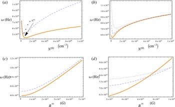
The angular frequency $({\it\omega})$ given by (2.13) is plotted in (a,b) against the number density $N^{(0)}$ for varying (a) electron relativistic parameter ${\it\eta}_{e}^{(0)}>0$ (solid curve) and ${\it\eta}_{e}^{(0)}\rightarrow 0$ (dashed curve) with $B^{(0)}=10^{12}~\text{G}$ (b) the magnetic field $B^{(0)}=2\times 10^{12}~\text{G}$ (solid curve), $3\times 10^{12}~\text{G}$ (dashed curve), $5\times 10^{12}~\text{G}$ (dotted curve). In (c,d) we plot the wave frequency versus the magnetic field $B^{(0)}$ for changing (c) ${\it\eta}_{e}^{(0)}>0$ (solid curve) and ${\it\eta}_{e}^{(0)}\rightarrow 0$ (dashed curve) when $N^{(0)}=10^{30}~\text{cm}^{-3}$ and for variation of (d) $N^{(0)}=10^{31}~\text{cm}^{-3}$ (solid curve), $2\times 10^{31}~\text{cm}^{-3}$ (dashed curve) and $3\times 10^{31}~\text{cm}^{-3}$ (dotted curve).

To examine the impact of degenerate electrons and associated relativistic effects on the linear dispersion of magnetosonic waves, we plot the angular frequency $({\it\omega})$ (2.13) against the equilibrium number density $N^{(0)}$ in figure 1(a). For ${\it\eta}_{e}^{(0)}>0$ , the solid curve indicates the electron relativistic correction which disappears for ${\it\eta}_{e}^{(0)}\rightarrow 0$ (dashed curve) which reduces the pressure law to equation (2.4). Note that the wave frequency decreases to a certain lowest possible value at a critical density value $N_{c}^{(0)}\sim 10^{30}~\text{cm}^{-3}$ (indicated with the dots/arrow). Beyond this value, the wave frequency increases when $N_{c}^{(0)}>N^{(0)}$ . We have also checked numerically that the Fermi acoustic speed $C_{Fs}\,[=(E_{Fe}/m_{i})^{1/2}]$ approaches the Alfvén speed at $N^{(0)}\sim N_{c}^{(0)}$ and exceeds it when $N^{(0)}>N_{c}^{(0)}$ . Hence ${\it\omega}$ decreases to a finite minimum value at $N_{c}^{(0)}$ and increases with further variation of number density. This result matches equation (27) in Hussain et al. (Reference Hussain, Mahmood and Rehman2014) where we believe that the wave frequency may decrease (increase) with number density when $V_{a}>C_{s}$ ( $V_{a}<C_{s}$ ). Overall, the relativistic electrons have considerable impact on the linear dispersion of magnetosonic waves and consequently suppress the wave frequency. Figure 1(b) shows the plot of ${\it\omega}$ versus plasma number density $N^{(0)}$ for different values of the external magnetic field, $B^{(0)}=2\times 10^{12}$ , $3\times 10^{12}$ and $5\times 10^{12}~\text{G}$ . It is obvious here that the minimum of ${\it\omega}$ is shifted to higher values of number density. To see the effect of the external magnetic field variation on ${\it\omega}$ at fixed plasma number density, we plot ${\it\omega}$ versus $B^{(0)}$ in figure 1(c) with fixed $N^{(0)}=10^{30}~\text{cm}^{-3}$ . The solid $({\it\eta}_{e}^{(0)}>0)$ and dashed $({\it\eta}_{e}^{(0)}\rightarrow 0)$ curves exhibit a clear departure at small values of $B^{(0)}$ , and are diminished at larger $B^{(0)}$ . This can be explained by the dispersion relation (2.13) in that at large values of the magnetic field $V_{A}\gg C_{_{Fs}}$ the curves saturate. Figure 1(d) illustrates a linear dispersion of magnetosonic waves versus the magnetic field in the range $2\times 10^{12}~\text{G}<B^{(0)}<10^{13}~\text{G}$ for ${\it\eta}_{e}^{(0)}=2.56$ (solid curve), ${\it\eta}_{e}^{(0)}=3.23$ (dotted curve) and ${\it\eta}_{e}^{(0)}=3.69$ (dashed curve). Here, the line crossing shows the effective increase in ${\it\omega}$ due to the external magnetic field when the degenerate electrons are weakly relativistic. It is therefore concluded that relativistic electrons tend to stabilize the wave frequency against the rapid increase due to the intensification of the magnetic field. 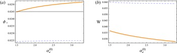The amplitude $({\it\phi}_{0})$ and width $(W)$ of the magnetosonic solitons are plotted against the energy ratio parameter $({\it\alpha}_{e}^{(0)})$ for varying electron relativistic parameter ${\it\eta}_{e}^{(0)}>0$ (solid curve) and ${\it\eta}_{e}^{(0)}\rightarrow 0$ (dotted curve) (see figure 2 a,b). Since the nonlinearity coefficient $(a_{1})$ is proportional to the inverse of the amplitude of the magnetosonic solitary waves, the relativistic pressure and electron degeneracy $({\it\alpha}_{e}^{(0)})$ lead to an enhancement of the wave amplitude by reducing the nonlinearity $(a_{1})$ of the system. 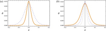Apart from nonlinearity, the parameters ${\it\alpha}_{e}^{(0)}$ and ${\it\eta}_{e}^{(0)}$ also significantly reduce the soliton width by affecting the phase $(V_{m})$ and Alfvén $(V_{A})$ speeds. Thus, the relativistic and degenerate electrons, through the Chandrasekhar equation of state, overcome the wave dispersion and can excite narrower magnetosonic solitons. To support this argument, we analyse the pulses of magnetosonic solitons numerically in figure 3(a) for ${\it\eta}_{e}^{(0)}>0$ (solid curve) and ${\it\eta}_{e}^{(0)}\rightarrow 0$ (dashed curve) which correspond to relativistic and non-relativistic pressures, respectively. A reduction in the wave dispersion and narrowing of the solitary wave are caused by incorporating the relativistic pressure (2.3) of the degenerate electrons. However, the enhancement of the values of ${\it\alpha}_{e}^{(0)}$ and ${\it\eta}_{e}^{(0)}$ leads to tapered solitary pulses, as shown in figure 3(b).

Figure 2.

The amplitude ${\it\phi}_{0}$ and width $W$ of magnetosonic solitons are plotted against ${\it\alpha}_{e}^{(0)}$ for ${\it\eta}_{e}^{(0)}>0$ (solid curve) and ${\it\eta}_{e}^{(0)}\rightarrow 0$ (dashed curve) with magnetic field $B^{(0)}=10^{12}~\text{G}$ .

Figure 3.

The profiles of magnetosonic solitary waves are depicted against spatial coordinate ${\it\chi}$ (a) with $B^{(0)}=10^{12}~\text{G}$ , $N^{(0)}=10^{31}~\text{cm}^{-3}$ and varying the electron relativistic parameter ${\it\eta}_{e}^{(0)}>0$ (solid curve), ${\it\eta}_{e}^{(0)}\rightarrow 0$ (dashed curve) and for different values of relativistic and degeneracy parameters (b) ${\it\eta}_{e}^{(0)}=1.19$ , ${\it\alpha}_{e}^{(0)}=0.7$ (solid curve), ${\it\eta}_{e}^{(0)}=2.03$ , ${\it\alpha}_{e}^{(0)}=2.07$ (dashed curve) and ${\it\eta}_{e}^{(0)}=4.38$ , ${\it\alpha}_{e}^{(0)}$ (dotted curve) at $B^{(0)}=10^{12}~\text{G}$ .

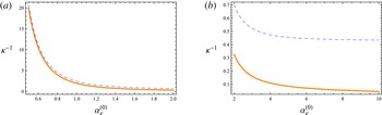
The width ${\it\kappa}^{-1}\;(=10a_{2}/a_{3})$ of the magnetosonic shock waves are presented in figure 4(a,b) against the energy ratio ${\it\alpha}_{e}^{(0)}$ for varying electron relativistic parameter ${\it\eta}_{e}^{(0)}>0$ (solid curve) and ${\it\eta}_{e}^{(0)}\rightarrow 0$ (dashed curve) corresponding to (2.3) and (2.4). As the electron relativistic pressure reduces the width $({\it\kappa}^{-1})$ , consequently it is deduced that the relativistic effect tends to spatially localize the shock waves, overcoming the wave dispersion which arises due to the displacement current. The wider departure of lines in figure 4(b) reveals a more significant impact on ${\it\kappa}^{-1}$ , when the electrons are strongly relativistic, i.e. $2<{\it\alpha}_{e}^{(0)}<10$ . 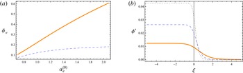Thus, it is concluded that a low density (comparatively) plasma admits wider magnetosonic shock waves due to wave dispersion, however, the relativistic electrons and pressure degeneracy favour a dense plasma permitting narrower shocks. The amplitude $({\it\Psi}_{0})$ of the magnetosonic shock is plotted against the energy ratio parameter in the range $0.7<{\it\alpha}_{e}^{(0)}<2.1$ in figure 5(a) for relativistic $({\it\eta}_{e}^{(0)}>0)$ and non-relativistic $({\it\eta}_{e}^{(0)}\rightarrow 0)$ pressures, respectively. It is obvious that an increase of the electron Fermi energy through the parameter ${\it\alpha}_{e}^{(0)}$ amplifies the strength of the shock wave. Moreover, the difference in the two curves shows an increase in the shock strength due to the relativistic pressure of the electrons. Thus, the relativistic and quantum degenerate electrons effectively modify the properties of the magnetosonic shock waves also. Solution (2.51) represents a monotonic profile of the shock in a travelling wave frame and is plotted against the spatial coordinate $-5<{\it\xi}<5$ (see figure 5 b). The solid, dashed and dotted curves correspond to ${\it\alpha}_{e}^{(0)}=1.12$ , 1.47, 1.78 with ${\it\eta}_{e}^{(0)}=1.49$ , 1.71 and 1.88. Note that the waves amplify and tend to spatially localize with an increase of ${\it\alpha}_{e}^{(0)}$ and ${\it\eta}_{e}^{(0)}$ . 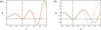Finally, to see the impact of the relativistic electrons and the energy ratio parameter on the oscillating shock waves, solution (2.54) is numerically examined in figure 6. We note from figure 6(a) that the solid curve lags behind the dashed curve, indicating a reduction in the wave dispersion and the spatial localization of the shock wave due to the relativistic pressure. Figure 6(b) displays the combined effects of relativistic electrons and the degeneracy pressure which strengthen the amplitude of the oscillatory shock.

Figure 4.

The width $({\it\kappa}^{-1})$ of the magnetosonic shock wave is shown against ${\it\alpha}_{e}^{(0)}$ in (a,b) for ${\it\eta}_{e}^{(0)}>0$ (solid curve) and ${\it\eta}_{e}^{(0)}\rightarrow 0$ (dashed curve) at $B^{(0)}=10^{12}~\text{G}$ .

Figure 5.

The amplitude of the magnetosonic shock is plotted versus ${\it\alpha}_{e}^{(0)}$ (a) with ${\it\eta}_{e}^{(0)}>0$ (solid curve) and ${\it\eta}_{e}^{(0)}\rightarrow 0$ (dashed curve) at magnetic field $B^{(0)}=2\times 10^{12}~\text{G}$ , whereas in (b) the monotonic profiles of the shock waves are shown against ${\it\xi}$ , for varying ${\it\eta}_{e}^{(0)}=1.49$ , ${\it\alpha}_{e}^{(0)}=1.12$ (solid curve), ${\it\eta}_{e}^{(0)}=1.71$ , ${\it\alpha}_{e}^{(0)}=1.47$ (dashed curve) and ${\it\eta}_{e}^{(0)}=1.88$ , ${\it\alpha}_{e}^{(0)}=1.78$ (dotted curve) at $B^{(0)}=5\times 10^{12}~\text{G}$ .

Figure 6.

The oscillatory shock wave solution from (2.54) is plotted versus ${\it\zeta}$ (a) for ${\it\eta}_{e}^{(0)}>0$ (solid curve) and ${\it\eta}_{e}^{(0)}\rightarrow 0$ (dotted curve) and (b) with different values of the relativistic parameter ${\it\eta}_{e}^{(0)}=1.19$ , ${\it\alpha}_{e}^{(0)}=0.708$ (solid curve), ${\it\eta}_{e}^{(0)}=1.26$ , ${\it\alpha}_{e}^{(0)}=0.80$ (dashed curve) and ${\it\eta}_{e}^{(0)}=1.49$ , ${\it\alpha}_{e}^{(0)}=1.12$ (dotted curve).

4. Summary

We have presented magnetosonic solitons and shocks in a dense magneto plasma, whose constituents are degenerate relativistic inertialess electrons and non-degenerate cold positive ions. The linear and nonlinear properties of the magnetosonic wave are modified by relativistic effects taken into account by using the generalized Chandrasekhar degeneracy pressure in the QMHD model. Numerical analysis reveals that the wave angular frequency decreases to its lowest value until a critical value of the number density is attained. After this, the wave frequency $({\it\omega})$ increases as the number density increases. The magnetic field also influences ${\it\omega}$ , such that the lowest possible frequency occurs at a higher number density when we intensify the magnetic field effects. In addition, the linear analysis shows that the relativistic electrons reduce the rapid increase in ${\it\omega}$ due to an increase in the external magnetic field (see figure 1). For the nonlinear analysis, the effectiveness of the parameters ${\it\eta}_{e}^{(0)}$ and ${\it\alpha}_{e}^{(0)}$ lead to the generation of narrower magnetosonic solitons in dense plasmas, propagating with lower dispersion (see figures 2 and 3). A strong impact of the relativistic electrons and pressure degeneracy is shown on the profiles of magnetosonic shocks, favouring a strengthening of the shocks. Furthermore, it reveals that ${\it\eta}_{e}^{(0)}$ and ${\it\alpha}_{e}^{(0)}$ modify the various plasma parameters and allow for the possibility of the formation of narrower shocks in magnetized dense relativistic plasmas (see figures 4–6).