



1. Introduction
The transition from laminar to turbulent flow profoundly influences drag and heat and mass transfer by altering flow and thermal resistance. This phenomenon remains a fundamental challenge in both advanced scientific research and large-scale engineering applications. Fluid machinery components, such as compressor and low-pressure turbine blades, generate a favourable–adverse pressure gradient within the boundary layer (Zaki et al. Reference Zaki, Wissink, Rodi and Durbin2010), a critical factor in transition. The fluid undergoes successive acceleration and deceleration, respectively thinning and thickening the boundary layer. The latter may induce boundary layer separation, leading to laminar separation bubbles, spanwise rollers and inflectional instability (Li & Yang Reference Karniadakis, Israeli and Orszag2019; Wang et al. Reference Verzicco2019b ). Beyond inherent pressure gradients, blades may acquire roughness due to erosion and deposition. Recent studies have extensively investigated roughness-induced transition in channels with pressure gradient. For example, Ishida et al. (Reference Hosseinverdi and Fasel2022) performed wind tunnel experiments on swept-back aerofoils with isolated cylinders, complemented by synchronous direct numerical simulations (DNS). Wang et al. (Reference Wang, Mao and Zaki2021) employed large-eddy simulations (LES) to analyse rough arrays on compressor blades, demonstrating their efficacy in enhancing streamwise vortex structures and accelerating separated shear layer instability, with increased roughness amplitude significantly reducing blade profile loss. De Vincentiis et al. (Reference De Tullio, Paredes, Sandham and Theofilis2022) conducted numerical simulations on aerofoils with regular roughness, while Jelly et al. (Reference Jelly and Busse2023) applied LES to low-pressure turbine blades with near-Gaussian rough surfaces. Given the complexity of engineering structures and the high Reynolds numbers involved, simulating actual blade boundary layers with body-fitted grids demands prohibitive computational costs. Further analysis of regular roughness or complex rough surfaces on this basis becomes impractical. Consequently, researchers have developed simplified schemes, such as employing a topographically deformed boundary (contraction–expansion section) to impose an equivalent favourable–adverse pressure gradient on a flat plate (Zhang & Hodson Reference Zaki, Wissink, Rodi and Durbin2006; Rao et al. Reference O’Rourke2014; Sivaramakrishnan Malathi et al. Reference Seddighi, He, Pokrajac, O’Donoghue and Vardy2022). Other methods impose variable pressure gradients by prescribing velocity distributions at the computational domain’s top horizontal boundary via the Falkner–Skan equation (Zoppini et al. Reference Zhang and Hodson2022; Nakagawa et al. Reference McKeon2023), which describes two-dimensional boundary layers under pressure gradients. This approach not only reduces computational costs, but also ensure orthogonal grids near the bottom wall, facilitating the application of the immersed boundary method, which excels in analysing complex solid walls.
Beyond the influence of favourable–adverse pressure gradients, roughness constitutes a substantial factor affecting the transition mechanisms. Two decades ago, engineers employed miniaturised vortex generators, composed of periodically arranged ramps, to manage transition on aerofoils (Shahinfar et al. Reference Schmid and Henningson2014; Bucci Reference Brandt2017). Nevertheless, the influence of these prevalent, modulated roughness arrays on transition and disturbance growth mechanisms remains incompletely understood. By contrast, the most comprehensively examined subject over the past two decades has been the isolated cylinder, the simplest and most representative roughness element. Its principal parameters are generally characterised by roughness height, aspect ratio and roughness Reynolds number. Previous research has exhaustively explored the coupled effects of these parameters on disturbance growth modes across various parameter ranges (Andersson et al. Reference Ananth, Nardini, Vaid, Kozul, Rao Vadlamani and Sandberg2001; Ergin & White Reference Dunn, Baran and Miatech2006; Vaughan & Zaki Reference Szumbarski and Floryan2011; Loiseau et al. Reference Ling, Wang, Huang and Xi2014; Puckert & Rist Reference Nikuradse2018; Bucci et al. Reference Bucci2021). Recently, the focus has increasingly shifted towards regular roughness arrays, with pertinent studies encompassing cubic arrays (Ma & Mahesh Reference Luo, Dai, de Sousa and Yin2023), hemispherical arrays (von Deyn et al. Reference Vaughan and Zaki2020) and pyramidal arrays (Seddighi et al. Reference Sandberg and Sandham2015). Concerning the fundamental units of the array, the adjacent roughness elements, researchers have begun to investigate their impact on the underlying mechanisms. Examples include the DNS and experimental work by Dong et al. (Reference Denissen and White2019) on spanwise-adjacent roughness elements, the Yang (Reference Wang, Ge, Deng, Yu and Wang2012) study of streamwise-adjacent hemispherical elements, and the research by Lu et al. (Reference Ling, Wang, Zhang, Gao and Xi2020a , Reference Loiseau, Robinet, Cherubini and Lericheb ) on the upstream–downstream interchange of bumps and rough strips. Given that the geometry of the roughness element is also a critical factor influencing flow stability and the structure of the flow field, Ling et al. (Reference Kellersmann, Weiler, Bode, Friedrichs, Stading and Ramm2024, Reference Li and Yang2025a ) have, in addition to inter-element spacing, also examined the effects of shape variations.
However, research concerning the actual rough surfaces on blades remains even more limited compared to that devoted to the aforementioned rough arrays. This is primarily attributable to the intricate height distribution of three-dimensional rough surfaces, which becomes exceedingly complex due to varying operating conditions and application scenarios (Dunn et al. Reference von Deyn, Forooghi, Frohnapfel, Schlatter, Hanifi and Henningson1996; Kellersmann et al. Reference Kang, Iaccarino and Moin2018; Gilge et al. Reference Fadlun, Verzicco, Orlandi and Mohd-Yusof2019), posing a significant challenge in summarising their key parameters. Presently, the most reliable parameters are the specific statistical metrics delineated by Chung et al. (Reference Cherubini, Robinet, De Palma and Alizard2021). In engineering applications, the equivalent sand-grain roughness introduced by Nikuradse (Reference Monokrousos, Åkervik, Brandt and Henningson1933) continues to be employed to address actual roughness. Bons (Reference Blackburn, Lee, Albrecht and Singh2010) synthesised empirical correlations between sand-grain roughness and measured roughness parameters in the gas turbine domain, yet observed substantial errors in many of these correlations. In fundamental research, Busse & Jelly (Reference Bucci, Cherubini, Loiseau and Robinet2023) examined the effects of positive and negative skewness on the roughness function, revealing that excessive positive skewness causes the roughness function, peak Reynolds stress and other characteristics to asymptotically approach constant values. Jelly et al. (Reference Jelly and Busse2022) investigated the influence of spanwise and streamwise effective slopes of three-dimensional irregular rough surfaces on wall turbulence, demonstrating that an increased ratio of these slopes reduces the recirculation zone behind local roughness peaks, while a larger spanwise effective slope markedly diminishes drag losses. Yang et al. (Reference Yang and Balaras2022) explored the sheltering effect of rectangular arrays, proposing a formula for calculating the sheltering angle, which enables direct evaluation of the relative magnitude of frictional resistance based on rough-surface geometry – a significant advancement for engineering applications. Ling et al. (Reference Ling, Gao, Wang, Zeng, Huang and Xi2025b ) further refined the accuracy of this predictive formula. Forooghi et al. (Reference Ericson2018) performed DNS on fully developed turbulence over three-dimensional irregular rough surfaces, comprehensively detailing the impact of root mean square height, skewness and kurtosis on flow-field statistics such as Reynolds stress. Additional studies have analysed spanwise-spaced rough stripes (Stroh et al. Reference Shahinfar, Sattarzadeh and Fransson2020), finding that the alternating distribution of smooth and rough surfaces induces secondary flows and additional drag. Beyond three-dimensional rough surfaces, related research extends to corrugated rough surfaces (Szumbarski & Floryan Reference Sivaramakrishnan Malathi, Nardini, Vaid, Rao Vadlamani and Sandberg2006) and stochastic rough surfaces (Ma et al. Reference Lu, Liu, Liu and Yan2021), among others.
Depending on its height, roughness may induce transition via the bypass transition route, which is governed by the transient growth of disturbances. Unlike the exponential growth characteristic of classical Tollmien–Schlichting waves, the transient growth mechanism exhibits a markedly higher linear amplification rate during the initial stages of disturbance evolution. This heightened growth readily leads to secondary instabilities within coherent structures, such as velocity streaks, ultimately culminating in the nonlinear progression of disturbances. Consequently, elucidating the spatial configuration of optimal disturbances – those with maximal energy growth rates – is paramount. Alizard et al. (Reference Åkervik, Brandt, Henningson, Hoepffner, Marxen and Schlatter2018) investigated transient optimal growth in the inlet zone, revealing that over short optimisation time, varicose wave packets amplify through synergistic interactions between the Orr and lift-up mechanisms. Conversely, over extended durations, both varicose and sinuous wave packets display instabilities driven by inflection points within the streaky flow. Wang et al. (Reference Wang, Lu, Yang, Zhao and Zhang2019a ) examined disturbance amplification mechanisms induced by an elliptical leading edge, while Huang et al. (Reference Gilge, Kellersmann, Friedrichs and Seume2021) incorporated plate vibrations to further explore transient growth dynamics. Ehrenstein & Gallaire (Reference Dong, Liu, Geng, Liu, Yang and Cheng2008) investigated the optimal perturbations in the rear of a two-dimensional bump, whereas Cherubini et al. (Reference Busse, Lutzner and Sandham2013) subsequently examined the global optimal perturbations elicited by smooth three-dimensional roughness elements within boundary layer flows. Beyond global disturbances, research has also focused on optimal perturbations at boundaries, exemplified by the foundational work of Mao et al. (Reference Ma and Mahesh2013) and their subsequent investigation into optimal inlet disturbances in stenotic flow (Mao et al. Reference Ma, Alamé and Mahesh2012). Complementary to transient growth analysis, resolvent analysis (McKeon Reference McKeon2017; Rolandi et al. Reference Puckert and Rist2024) offers an alternative framework by applying harmonic forcings to study disturbance evolution within linearised systems. This approach effectively models nonlinear interactions arising from highly amplified coherent structures, thereby identifying the most energetic motions in turbulent flows. Bae et al. (Reference Andersson, Brandt, Bottaro and Henningson2021) employed resolvent analysis to quantify the impact of principal forcing modes on coherent structures in the buffer and logarithmic layers of wall turbulence, whereas Monokrousos et al. (Reference Martini, Rodríguez, Towne and Cavalieri2010) performed a global harmonic forcing analysis for the Blasius boundary layer. In the context of roughness, Bucci et al. (Reference Bucci2021) concurrently analysed optimal disturbances and harmonic forcing in a flat-plate boundary layer subjected to free-stream turbulence and isolated cylinders. Notably, non-modal and resolvent analysis of three-dimensional rough surfaces and flows under variable pressure gradients remains unexplored in the current literature.
For this type of flow, the current research has elucidated the influence of three-dimensional rough surface parameters – including height, effective slope and skewness – on drag and near-wall coherent structures (Szumbarski & Floryan Reference Sivaramakrishnan Malathi, Nardini, Vaid, Rao Vadlamani and Sandberg2006; Ehrenstein & Gallaire Reference Dong, Liu, Geng, Liu, Yang and Cheng2008; Wang et al. Reference Wang, Lu, Yang, Zhao and Zhang2019a ; Huang et al. Reference Gilge, Kellersmann, Friedrichs and Seume2021). Our prior work (Ling et al. Reference Ling, Gao, Wang, Zeng, Huang and Xi2025b ,Reference Ling, Wang, Huang, Gao and Xi d ) comprehensively investigated the effects of surface skewness, isotropy/anisotropy, and streamwise arrangement on resistance characteristics and downstream transition flow structures, such as linear modes and secondary flows. Building on this foundation, the next critical step is to investigate the intrinsic disturbance growth mechanisms in transitional flows over three-dimensional rough surfaces under variable pressure gradients. This study aims to establish a unified framework for global stability across varying rough-surface parameters, and to analyse key properties of optimal disturbances and harmonic forcing, including spatial distribution and energy growth rates. Accordingly, this paper designs isotropic and anisotropic rough surfaces with negative skewness, positioned upstream of the separation point. Three methodologies – global stability analysis, local transient growth analysis and resolvent analysis – are employed to elucidate the effects of different parameters on disturbance growth. § 2 details the computational domain, rough-surface configurations and analytical methods. § 3 presents and discusses the numerical results. § 4 concludes the study.
(a) The computational domain encompasses a three-dimensional rough surface subjected to a variable pressure gradient. The rough surface is positioned upstream of the separation point, and both the front and rear ends of the rough surface are transitioned by buffer slopes. A buffer region is strategically placed near the outlet to mitigate backflow and maintain the fidelity of the upstream flow field. The outlet boundary is characterised by fully developed flow conditions, while the bottom wall adheres to a no-slip condition. Notably, the lowest elevation of the rough surface remains flush with the bottom wall across all cases. The spanwise boundaries are periodic boundaries. The rough surface investigated herein exhibits either isotropic or anisotropic properties with negative skewness. (b) The inlet and top boundaries of the computational domain are prescribed with specific velocity distributions in the streamwise and wall-normal directions. (c) The spanwise power spectra of the three rough surfaces are presented, where
 $\beta$
represents the spanwise wavenumber. (d) The distribution of bottom-wall pressure coefficient along the streamwise direction in the absence of rough surface is presented,
 ${{C}_{\!p}}=( p-{{p}_{\textit{in}}} )/( \rho U_{\infty }^{2}/2 )$
, with
 $p_{\textit{in}}$
denoting the inlet pressure.

Figure 1. Long description
Panel A: The diagram depicts a three-dimensional computational domain with a rough surface subjected to a variable pressure gradient. The rough surface is positioned upstream of the separation point, with buffer slopes at both ends. A buffer region is placed near the outlet to maintain flow fidelity. The outlet boundary has fully developed flow conditions, and the bottom wall adheres to a no-slip condition. The rough surface can exhibit either isotropic or anisotropic properties with negative skewness. Panel B: Two line graphs show the velocity distributions at the inlet and top boundaries of the computational domain. The inlet boundary graph plots the streamwise (u/U∞) and wall-normal (v/U∞) velocity components against the vertical axis (y/H). The top boundary graph plots the streamwise (u/U∞) and wall-normal (v/U∞) velocity components against the horizontal axis (x/H). Panel C: A line graph presents the spanwise power spectra of three rough surfaces, with the spanwise wavenumber (β) on the horizontal axis and the power spectral density (Phh) on the vertical axis. Three different lines represent different rough surface types. Panel D: A line graph shows the distribution of the bottom-wall pressure coefficient (Cp) along the streamwise direction (x/H) in the absence of a rough surface.
2. Numerical methods and model
2.1. Computational domain set-up and rough-surface synthesis
The computational domain of this model is depicted in figure 1(a), wherein
 $x$
,
 $y$
and
 $z$
denote the streamwise, wall-normal and spanwise directions, respectively. The domain design is adapted from the model used by Hosseinverdi & Fasel (Reference Forooghi, Stroh, Schlatter and Frohnapfel2019). All length scales are non-dimensionalised by half the wall-normal height of the computational domain,
 $H=1$
. As illustrated in figure 1(b), the top boundary is a far-field condition with a constant free-stream velocity
 ${U}_{\infty }=1$
, and all velocity scales in this study are non-dimensionalised by
 ${U}_{\infty }$
. A prescribed wall-normal velocity distribution induces a favourable–adverse pressure gradient, while the inlet velocity profile is determined by the Falkner–Skan equation. The bottom boundary is a no-slip flat wall. The outlet velocity field is subject to zero Neumann boundary conditions, whereas the outlet pressure field is subject to zero Dirichlet boundary conditions. The spanwise boundaries are periodic. The adequacy of the wall-normal and spanwise extents of the computational domain has been validated in our prior work (Ling et al. Reference Ling, Gao, Wang, Zeng, Huang and Xi2025b
). It has been demonstrated that the Dirichlet condition imposed on the streamwise velocity at the top boundary does not introduce non-physical constraints or spurious vorticities within the boundary layer. To avoid the excessive influence of the abrupt front and rear ends of rough surface on the flow field, this study incorporates a smooth buffer slope, following the approach of Ananth et al. (Reference Alizard, Cadiou, Le Penven, Di Pierro and Buffat2023). The cosine profile of the buffer is adopted from the work of Sandberg & Sandham (Reference Rao, Jefferson-Loveday, Tucker and Lardeau2006). The height of the buffer slope for each rough surface is determined based on its effective height – defined as the ratio of the total volume occupied by the rough surface to the projected area on the bottom wall – while the streamwise length of the buffer slope is fixed at 20 % of the rough surface length. The specific statistical characteristics can be found in table 1.
Statistical characteristics of rough surfaces:
 $h_{avg}$
denotes the average height;
 $h_{\textit{rms}}$
represents the root mean square height;
 ${\textit{Sk}}$
indicates the skewness;
 ${\textit{Ku}}$
signifies the kurtosis;
 $\textit{ES}_x$
defines the effective streamwise slope;
 $\textit{ES}_z$
defines the effective spanwise slope;
 $h_{\textit{max}}$
denotes the maximum elevation;
 $h_{\textit{min}}$
denotes the minimum elevation;
 $h_{\textit{eff}}$
represents the effective height, defined as the total volume occupied by the rough surface normalised by its projected area on the bottom wall;
 $\delta _{99,\textit{in}}$
denotes the inlet boundary layer thickness, corresponding to the height where the streamwise velocity attains
 $0.99U_\infty$
;
 $\delta _{\textit{in}}^{*}$
signifies the inlet displacement thickness;
 $\delta _{99,r}$
represents the mean boundary layer thickness across the rough surface coverage domain;
 $\delta _{99,\textit{front}}$
,
 $\delta _{99,\textit{mid}}$
and
 $\delta _{99,\textit{rear}}$
denote the boundary layer thicknesses at the leading edge, streamwise centre and trailing edge of the rough surface coverage, respectively, along the spanwise centreline;
 $L_r$
specifies the streamwise length of the rough surface. The thickness parameters in the final five rows are derived from results at
 $\textit{Re} = 600$
.

Table 1. Long description
A table comparing statistical properties of rough surfaces across three different cases: ER0, ER1, and ER2. The table has 15 rows and 4 columns. The columns are labeled Statistical properties, ER0, ER1, and ER2. The rows list various statistical properties and their corresponding values for each case. Row 1: h_avg/H, 0, 0.015, 0. Row 2: h_rms/H, 0, 0.015, 0. Row 3: Sk, -1.421, -1.396, -1.445. Row 4: Ku, 6.909, 6.747, 7.113. Row 5: ES_x/H, 0.209, 0.213, 0.186. Row 6: ES_y/H, 0.109, 0.214, 0.445. Row 7: ES_z/ES_x, 0.520, 1.004, 2.394. Row 8: (h_max - h_min)/H, 0.139, 0.150, 0.151. Row 9: h_eff/H, 0.105, 0.110, 0.113. Row 10: h_eff/δ99_in, 0.556, 0.583, 0.599. Row 11: h_eff/δ99_x, 1.589, 1.664, 1.710. Row 12: h_eff/δ99_r, 0.544, 0.554, 0.563. Row 13: Lr/δ99_front, 6.254, 6.156, 6.131. Row 14: Lr/δ99_mid, 5.015, 4.869, 4.819. Row 15: Lr/δ99_r, 5.179, 5.039, 4.979.
This study employs the methodology established by Yang et al. (Reference Yang2014) to generate rough surfaces characterised by specific statistical moments and autocorrelation functions. The first four moments – mean height, root mean square height, skewness and kurtosis – quantify surface topography, while the autocorrelation function delineates the streamwise and spanwise wavelengths. To enhance numerical convergence, the generated surface matrix undergoes low-pass Fourier filtering, yielding a smoothly varying three-dimensional surface (Jelly & Busse Reference Huang, Xiao, Ren, Wang, Xi and Mao2018, Reference Ishida, Ohira, Hosoi, Tokugawa and Tsukahara2019). This process involves a two-dimensional Fourier transformation along the streamwise and spanwise directions, truncation of high-wavenumber components via a circular low-pass filter, and subsequent inverse Fourier transformation. The filtering eliminates the smallest-scale features, mitigating excessive grid resolution and DNS costs, while ensuring periodic boundary conditions at the surface spanwise edges. Central to this operation is determining the cut-off wavenumber
 ${k}_{c}$
, estimated from the original streamwise (
 ${k}_{xs}$
) and spanwise (
 ${k}_{zs}$
) wavenumbers in Fourier space, with
 ${k}_{c}$
set to
 $k_{cs}^{2}={{ ( {{k}_{xs}}+2 )}^{2}}+{{ ( {{k}_{zs}}+2 )}^{2}}$
. This approach preserves surface similarity while achieving periodicity and scale reduction. A negatively skewed surface is selected, as prior research (Ling et al. Reference Ling, Gao, Wang, Zeng, Huang and Xi2025b
) demonstrated its superior efficacy in triggering transition compared to zero- or positively skewed surfaces. The parameter
 ${\textit{ER}} = {\textit{ES}_{z}}/{\textit{ES}_{x}}$
in figure 1(a) denotes the ratio of spanwise to streamwise effective slope (where effective slope is defined as the absolute value of the average streamwise or spanwise gradient of the height,
 ${\textit{ES}_{x}}={{A}^{-1}}\int _{A}{| \partial h/\partial x |\,\text{d}A}$
,
 ${\textit{ES}_{z}}={{A}^{-1}}\int _{A}{ | \partial h/\partial z |\,\text{d}A}$
, where
 $A$
is the projected area of the rough surface on the bottom wall, and
 $h$
is the height of the rough surface), with higher values indicating more pronounced spanwise modulation. Three values of this parameter (0.52, 1.00, and 2.40) are investigated, corresponding to surfaces ER0 (anisotropic), ER1 (isotropic), and ER2 (anisotropic), respectively. This study examines nine cases, utilising a Reynolds number defined by
 $H$
and
 $U_\infty$
, with the three rough surfaces designated as
 $\textit{Re}=600,800,1000$
. When the inlet boundary layer thickness serves as the reference length, the corresponding Reynolds number conversions are presented in table 2.
Thicknesses of the inlet boundary layer and the corresponding Reynolds numbers, where
 $\theta _{\textit{in}}$
represents the momentum thickness at the inlet.

Table 2. Long description
The table presents a comparison of different references at Reynolds numbers of 600, 800, and 1000. It includes six rows and four columns. The columns are labeled as Different references, Re = 600, Re = 800, and Re = 1000. The rows are labeled as δ99,in/H, δin*/H, θin/H, Reδ99,in, Reδin*, and Reθin. The values in the table are as follows: Row 1: δ99,in/H, 0.189, 0.066, 0.026. Row 2: δin*/H, 113, 151, 189. Row 3: θin/H, 40, 53, 66. Row 4: Reδ99,in, 15, 20, 26.
2.2. The DNS and embedded boundary method
This paper employs DNS to solve the incompressible Navier–Stokes (NS) equations
 \begin{equation} \frac {\partial \boldsymbol{u}}{\partial t}+\left ( \boldsymbol{u}\boldsymbol{\cdot }\boldsymbol{\nabla }\right )\boldsymbol{u}=-\frac {\boldsymbol{\nabla }\!p}{\rho }+\nu\, {{{\nabla} }^{2}}\boldsymbol{u}+\boldsymbol{f}, \end{equation}
in which
 $\boldsymbol{u}$
is the velocity,
 $t$
denotes time,
 $\nu$
represents the fluid kinematic viscosity,
 $p$
signifies pressure,
 $\rho$
indicates density, and
 $\boldsymbol{f}$
denotes the forcing term.
The DNS solver utilised in this study is Semtex (Blackburn et al. Reference Barkley, Blackburn and Sherwin2019), which employs the spectral element method renowned for its high accuracy, and incorporates a stiffly stable algorithm for temporal integration (Karniadakis et al. Reference Jelly, Ramani, Nugroho, Hutchins and Busse1991). The rough surfaces are resolved using the embedded boundary method (EBM) (Verzicco Reference Vanella and Balaras2023), a technique extensively investigated in prior research (Fadlun et al. Reference Ergin and White2000; Kang et al. Reference Jelly, Nardini, Rosenzweig, Leggett, Marusic and Sandberg2009; Vanella & Balaras Reference Stroh, Schafer, Frohnapfel and Forooghi2009; Luo et al. Reference Lu, Liu, Liu and Yan2012). Even for a Semtex solver necessitating a homogeneous spanwise domain, the immersed-boundary-method nature of the EBM intrinsically captures the influence of heterogeneous three-dimensional rough surfaces upon the flow field. This effect manifests as non-uniform velocity values across uniformly distributed nodes in the spanwise direction. Specifically, this paper implements the EBM following the methodology outlined by Yang & Balaras (Reference Yang, Stroh, Chung and Forooghi2006):
 \begin{equation} \frac {{{\gamma }_{0}}}{\Delta t}\big ( \overset \frown {\boldsymbol{u}}-{\boldsymbol{u}^{*}} \big )={\boldsymbol{f}^{\textit{EBM}}}, \end{equation}
 \begin{equation} \frac {{{\gamma }_{0}}}{\Delta t} \big( {\boldsymbol{u}^{n+1}}-\overset \frown {\boldsymbol{u}} \big )=-\boldsymbol{\nabla }\overset \frown {p}, \end{equation}
in which
 ${\gamma }_{0}$
denotes the coefficient in the temporal integration scheme, while
 $\Delta t$
represents the time step. The term
 $\overset \frown {\boldsymbol{u}}$
corresponds to the corrected velocity field,
 $\boldsymbol{u}^{*}$
to the original velocity field unaffected by the rough surface, and
 $\boldsymbol{u}^{n+1}$
to the velocity field to be updated for the subsequent temporal layer. The variables
 $\boldsymbol{f}^{\textit{EBM}}$
and
 $\overset \frown {p}$
respectively signify the volumetric force induced by the rough surface and the resultant pressure perturbation. The synergistic influence of
 $\boldsymbol{f}^{\textit{EBM}}$
and
 $\overset \frown {p}$
ensures the incompressibility of
 $\boldsymbol{u}^{n+1}$
. By adding and applying the divergence to (2.2) and (2.3), the Poisson equation governing
 $\overset \frown {p}$
is derived:
 \begin{equation} {{{\nabla} }^{2}}\overset \frown {p}=\boldsymbol{\nabla }\boldsymbol{\cdot }{\boldsymbol{f}^{\textit{EBM}}}. \end{equation}
Given the known corrected velocity field
 $\overset \frown {\boldsymbol{u}}$
, and the original velocity and pressure fields excluding the influence of the rough surface, the forcing
 $\boldsymbol{f}^{\textit{EBM}}$
can be determined. Subsequently,
 $\overset \frown {p}$
is computed using (2.2) and (2.4), while
 $\boldsymbol{u}^{n+1}$
is derived from (2.3). The pressure field for the subsequent update layer is then obtained via the formula
 \begin{equation} p={{p}^{*}}+\overset \frown {p}, \end{equation}
in which
 ${p}^{*}$
denotes the original pressure field devoid of any perturbations induced by the rough surface. Notably, this study employs a quadrilateral mesh, rather than a triangular mesh (O’Rourke Reference Nakagawa, Tsukahara and Ishida1998; Ericson Reference Ehrenstein and Gallaire2005; Yang Reference Yang, Li, Wang and Hong2016), to resolve the solid wall, owing to its geometric compatibility with canonical shapes such as cuboids, cylinders and spheres. Furthermore, the iterative methodology advanced by Busse et al. (Reference Busse and Jelly2015) is integrated, thereby streamlining the implementation of the EBM within DNS.
2.3. Global stability and optimal growth analyses
Global stability analysis, performed under the assumption of a prescribed three-dimensional base flow, investigates the evolution of perturbations within the flow field through the lens of the linearised NS equations. These equations are derived by subtracting the Reynolds-averaged equations from (2.1) and subsequently discarding the nonlinear terms:
 \begin{equation} \frac {\partial {\boldsymbol{u}}'}{\partial t}+\left ( \boldsymbol{U}\boldsymbol{\cdot }\boldsymbol{\nabla }\right ){\boldsymbol{u}}'+\left ( {\boldsymbol{u}}'\boldsymbol{\cdot }\boldsymbol{\nabla }\right )\boldsymbol{U}=-\frac {\boldsymbol{\nabla }\!{p}'}{\rho }+\nu\, {{{\nabla} }^{2}}{\boldsymbol{u}}', \end{equation}
in which
 $\boldsymbol{u}'$
denotes the disturbance velocity,
 $\boldsymbol{U}$
is the base flow velocity, which is a steady solution of (2.1), and
 ${p}'$
is the disturbance pressure. The analysis of linear systems invariably necessitates the solving of the eigenpairs of the linear operator. However, for large-scale three-dimensional problems, the explicit computation of eigenpairs proves impractical. Consequently, matrix-free approaches are required. This study employs the time-stepping method to implement the linear operator in (2.6), with the Arnoldi algorithm utilised to determine the operator’s eigenpairs. Equation (2.6) can thus be reformulated as the eigenvalue problem
 \begin{equation} \frac {\partial \boldsymbol{u}'}{\partial t}=\boldsymbol{A}\boldsymbol{u}', \end{equation}
 \begin{equation} \boldsymbol{u}'\left ( \boldsymbol{x},t \right )={{\rm e}^{\boldsymbol{A}t}}\,\boldsymbol{u}'\left ( \boldsymbol{x},0 \right )=\boldsymbol{M}\,\boldsymbol{u}'\left ( \boldsymbol{x},0 \right ), \end{equation}
in which the operator
 $\boldsymbol{A}$
represents the linear NS operator constructed around the full three-dimensional base flow. Assuming that the linear operator
 $\boldsymbol{A}$
possesses the eigenvalue
 ${{\lambda }_{\!j}}={{\sigma }_{\!j}}+{\rm i}{{\omega }_{\!j}}$
,
 ${\sigma }_{\!j}$
represents the linear growth rate, and the operator
 $\boldsymbol{M}$
exhibits the eigenvalue
 ${\mu }_{\!j}$
, their interrelationship is defined by
 ${{\mu }_{\!j}}={{\rm e}^{{{\lambda }_{\!j}}t}}$
. The Arnoldi algorithm generates a sequence of Krylov subspaces through successive applications of
 $\boldsymbol{M}$
to the
 $\boldsymbol{u}'$
, ultimately converging on the eigenvalue
 ${\lambda }_{\!j}$
of
 $\boldsymbol{A}$
to analyse the linear stability of the flow. The base flow requisite for global stability analysis must satisfy temporal asymptotic stability. This study employs the selective frequency damping (SFD) method to compute the base flow (Åkervik et al. Reference Zoppini, Ragni and Kotsonis2006), which involves introducing a relaxation term proportional to the high-frequency velocity fluctuations into the NS equations. Notably, this approach demonstrates efficacy even for unsteady flows, such as those over aerodynamic wings.
Under conditions of linear asymptotic stability, the non-transposedness inherent in the linear NS operator generally results in non-normal eigenvectors. This implies that while any given perturbation will ultimately decay over an extended duration, it may initially undergo transient growth prior to attenuation. Should this transient growth attain a sufficient amplitude, the perturbation can transition from a linear to a nonlinear regime, thereby precipitating flow transition. The focal point of such analysis is the identification of the ‘most dangerous’ or ‘optimal’ initial perturbation, defined as the configuration that maximises growth amplitude within a specified time
 $T$
. To address this optimisation problem, it is necessary to introduce the following energy-type integrals or norms, and their corresponding growth rates:
 \begin{equation} E=\big ( {{\boldsymbol{u}}_{i}'},{{\boldsymbol{u}}_{\!j}'} \big )=\int _{V}{{\boldsymbol{u}}_{i}'}\boldsymbol{\cdot }{\boldsymbol{u}}_{\!j}'\,\text{d}V, \end{equation}
 \begin{equation} G=\underset {\boldsymbol{u}_{0}'}{\mathop {\max }}\,\frac {E\left ( T \right )}{E\left ( 0 \right )}=\underset {\boldsymbol{u}_{0}'}{\mathop {\max }}\,\frac {\left ( {\boldsymbol{u}_{T}'},{\boldsymbol{u}_{T}'} \right )}{\left ( {\boldsymbol{u}_{0}'},{\boldsymbol{u}_{0}'} \right )}=\underset {\boldsymbol{u}_{0}'}{\mathop {\max }}\,\frac {\left ( \boldsymbol{M}{\boldsymbol{u}_{0}'},\boldsymbol{M}{\boldsymbol{u}_{0}'} \right )}{\left ( {\boldsymbol{u}_{0}'},{\boldsymbol{u}_{0}'} \right )}. \end{equation}
According to the optimisation conditions of the Lagrangian functional, the above energy growth rate can be transformed into the form
 \begin{equation} G=\underset {\boldsymbol{u}_{0}'}{\mathop {\max }}\,\frac {\left ( \boldsymbol{M}{\boldsymbol{u}_{0}'},\boldsymbol{M}{\boldsymbol{u}_{0}'} \right )}{\left ( {\boldsymbol{u}_{0}'},{\boldsymbol{u}_{0}'} \right )}=\underset {\boldsymbol{u}_{0}'}{\mathop {\max }}\,\frac {\left ( {\boldsymbol{u}_{0}'},{{\boldsymbol{M}}^{+}}\boldsymbol{M}{\boldsymbol{u}_{0}'} \right )}{\left ( {\boldsymbol{u}_{0}'},{\boldsymbol{u}_{0}'} \right )}. \end{equation}
Equation (2.10) is mathematically equivalent to the eigenvalue problem
 ${\boldsymbol{M}^{+}}\boldsymbol{M}{\boldsymbol{u}_{0}'}=G{\boldsymbol{u}_{0}'}$
, enabling the application of the same algorithm utilised in the global stability analysis to perform the transient growth analysis of the perturbation. The sole modification lies in substituting matrix
 $\boldsymbol{M}$
for
 ${\boldsymbol{M}^{+}}\boldsymbol{M}$
as the eigenvalue matrix, and we employ the direct–adjoint iteration to facilitate the repeated evolution of this operator (Barkley et al. Reference Bae, Lozano-Durán and McKeon2008). In contrast to the linear NS equations, the adjoint equations differ only in the inclusion of time derivative and convection terms with reversed signs; all other terms remain unchanged. Consequently, it is very convenient to integrate these two equations to apply operators
 $\boldsymbol{M}$
and
 $\boldsymbol{M}^{+}$
. In conducting global stability and transient growth analyses for the proposed model, the convergence threshold for the leading eigenvalue is established at
 ${10}^{-7}$
. In the computation of the global modes and the optimal perturbations, the inlet, top and bottom must be prescribed with a zero Dirichlet velocity field and a zero Neumann pressure field, whereas the outlet requires a zero Neumann velocity field and a zero Dirichlet pressure field. These boundary conditions are essential to preclude the introduction of unnecessary perturbations. The convergence of the base flow using the SFD method and of the global modes is discussed in Appendix A.
2.4. Resolvent analysis
Subsequently, we will investigate the response and amplification of the linear NS operator elicited by a solitary harmonic forcing at a prescribed frequency (Monokrousos et al. Reference Martini, Rodríguez, Towne and Cavalieri2010; Martini et al. Reference Mao, Blackburn and Sherwin2021). The explicit formulation is
 \begin{equation} \frac {\partial \boldsymbol{u}'}{\partial t}=\boldsymbol{A}\boldsymbol{u}'+\boldsymbol{g}, \end{equation}
 \begin{equation} \boldsymbol{u}'\!\left ( \boldsymbol{x},t \right )=\int _{-\infty }^{\infty }{{{\widehat {\boldsymbol{u}}}_{\omega }}\!\left ( \boldsymbol{x} \right ) {{\rm e}^{-{\rm i}\omega t}}\,\text{d}\omega },\quad\boldsymbol{g}\!\left ( \boldsymbol{x},t \right )=\int _{-\infty }^{\infty }{{{\widehat {\boldsymbol{g}}}_{\omega }}\!\left ( \boldsymbol{x} \right )\,{{\rm e}^{-{\rm i}\omega t}}\,\text{d}\omega }, \end{equation}
in which
 $\boldsymbol{g}$
represents the volumetric force field modelling the nonlinear terms in the right-hand side of (2.12) as a harmonic forcing. Analogous to the global stability analysis in the preceding subsection, the present resolvent analysis is likewise centred upon the three-dimensional base flow. When analysing forcing and response perturbations, their spatial distribution is of primary interest; thus the shape function component can be isolated accordingly:
 \begin{equation} -{\rm i}\omega\, {{\widehat {\boldsymbol{u}}}_{\omega }}\!\left ( \boldsymbol{x} \right )=\boldsymbol{A}\,{{\widehat {\boldsymbol{u}}}_{\omega }}\!\left ( \boldsymbol{x} \right )+{{\widehat {\boldsymbol{g}}}_{\omega }}\!\left ( \boldsymbol{x} \right )\!. \end{equation}
After further derivation, one can obtain
 \begin{equation} {{\widehat {\boldsymbol{u}}}_{\omega }}\!\left ( \boldsymbol{x} \right )={{\left [ -{\rm i}\omega \boldsymbol{I}-A \right ]}^{-1}}\, {{\widehat {\boldsymbol{g}}}_{\omega }}\!\left ( \boldsymbol{x} \right )={\boldsymbol{H}_{\omega }}\,{{\widehat {\boldsymbol{g}}}_{\omega }}\!\left ( \boldsymbol{x} \right )\!, \end{equation}
in which
 $\omega$
denotes the circular frequency,
 $\boldsymbol{I}$
represents the identity matrix, the superscript
 $-1$
indicates the matrix inverse, and
 $\boldsymbol{H}_{\omega }$
signifies the resolvent operator. Equation (2.15) reveals that applying the eigenvalue method employed in transient growth analysis yields the optimal forcing and its corresponding response at a specified frequency
 $\omega$
. Consequently, the ratio of the response’s energy norm to that of the forcing reaches its maximum. Unlike global stability and transient growth analyses, resolvent analysis, as stipulated by (2.13), necessitates the flow to attain a quasi-periodic state, thereby satisfying the harmonic assumption (Martini et al. Reference Mao, Blackburn and Sherwin2021). This implies that following the onset of each direct integration or adjoint integration, a relaxation period is required to allow flow characteristics, such as global kinetic energy, to converge to a near-constant value. The response term
 ${{\widehat {\boldsymbol{u}}}_{\omega }} ( \boldsymbol{x} )$
and forcing term
 ${{\widehat {\boldsymbol{g}}}_{\omega }} ( \boldsymbol{x} )$
in (2.15) are derived using Fourier series during each integration cycle. Specifically, the continuous superposition of the product of response flow field at each time step and sinusoidal functions is necessitated to derive the Fourier series coefficients (i.e. forcing term) for each respective frequency. To efficiently compute the optimal harmonic forcing across multiple frequencies within a single calculation, the Krylov subspaces for each frequency can be archived as binary files. By selectively performing Arnoldi iteration on the subspace of a single frequency at a time, and implementing a storage–read loop, the computational memory demands are significantly minimised. Furthermore, forcings often exhibit substantial amplification prior to eigenvalue convergence, potentially reaching several orders of magnitude or even exceeding ten. Empirical investigations reveal that this phenomenon frequently induces divergence in the internal iterations of the EBM. To mitigate this issue, normalisation techniques are employed, effectively averting such divergence. Specifically, the velocity field undergoes normalisation while preserving its amplitude before each integration step, followed by amplitude restoration post-integration. The findings demonstrate that this approach constitutes an effective solution to the aforementioned challenge.
The distribution of the global leading growth rate across varying rough surfaces and Reynolds numbers, wherein the filled colours and adjacent numerical values denote the respective growth rates.

(a) The streamwise velocity contours of the base flows on the
 $x$
-slices and
 $z$
-slices. (b) Global stability leading mode streamwise velocity isosurfaces (
 $z$
-slices) and spanwise velocity isolines (
 $y$
-slices). The spanwise velocity background illustrates the base flow streamwise velocity distribution in the
 $y=0.16$
section, ranging from 0.1 (black) to 0.7 (white) with step size 0.06. For enhanced visualisation, the wall-normal and streamwise directions have been scaled by ratio 2 : 1. (c) The spatial distribution of the leading mode streamwise velocity at
 $x=5$
under the three cases corresponding to
 $\textit{Re}=1000$
. The two isolines delineate the wall-normal (dashed lines) and spanwise (solid lines) shear components of the base flow, respectively.

Figure 3. Long description
Panel A: Three sets of 3D contour plots show streamwise velocity distributions at different Reynolds numbers (Re = 600, 800, 1000) and expansion ratios (ER1, ER0, ER2). The color scale ranges from 0 to 1.2, indicating velocity ratios. Panel B: Three sets of 3D isosurfaces and 2D isolines illustrate the global stability leading mode streamwise velocity and spanwise velocity distributions. The background color scale ranges from 0.1 to 0.7, showing base flow streamwise velocity. Panel C: Three contour plots display the spatial distribution of the leading mode streamwise velocity at a specific condition, with isolines indicating wall-normal and spanwise shear components of the base flow.
3. Results
3.1. Global stability
When the Reynolds number surpasses the critical threshold, infinitesimal perturbations precipitate linear instability, leading to exponential amplification on the base flow. Prior to systematically elucidating the effects of varying rough surface parameters on disturbance evolution, it is imperative to rigorously quantify the linear stability of the flow for each considered Reynolds number and rough surface. This can be assessed by evaluating the linear growth rate of the leading mode, defined as the real part of the eigenvalue exponent, as depicted in figure 2. All nine cases investigated herein exhibit global stability with frequency zero. With increasing Reynolds number, the linear growth rates of the three rough surfaces all escalate, albeit with distinct gradients. Case ER1 exhibits the steepest gradient, while ER0 shows the most gradual. This observation suggests that isotropic rough surfaces are most prone to inducing linear instability at the global scale, followed by anisotropic surfaces with spanwise modulation, whereas surfaces with streamwise modulation demonstrate the strongest inertia in this regard.
The spatial distribution of the leading mode under various cases is illustrated in figure 3(b). Figure 3(a) illustrates the base flow structure for each case. At low Reynolds numbers with high linear stability, the streamwise and spanwise peak velocities of the leading mode for all three rough surfaces are predominantly concentrated near the outlet, exhibiting uniform streamwise velocity distribution in the spanwise direction. The spanwise wavenumber of the spanwise velocity distribution approximates unity, closely resembling the leading stable mode observed in favourable–adverse pressure gradient boundary layers investigated by Cherubini et al. (Reference Cherubini, De Tullio, De Palma and Pascazio2010). However, the current study reveals that disturbances induced by the rough surface prevent laminar separation bubble formation, resulting solely in convective-type wave packets near the outlet. With increasing Reynolds number, the spanwise velocity undergoes initial modifications, as evidenced by the ER1 distribution under
 $\textit{Re}=800$
conditions. Downstream regions of the rough surface begin generating new spanwise velocity wave packets. The spatial extent of such a wave packet is approximately 3–4 times the rough surface streamwise length, whereas the wavelength of the classical Tollmien–Schlichting wave,
 ${{\lambda }_{x}}=20{{\delta }^{*}}$
(evaluated via the displacement thickness proximal to the wave packet), constitutes approximately four times the rough surface streamwise length, exhibiting an intriguing concordance between the two. Further elevation of the Reynolds number to 1000 expands the spatial extent and complexity of these wave packets. Concurrently, a new peak region, analogous to a laminar separation bubble, emerges in the streamwise velocity distribution at the spanwise centre – a phenomenon exclusive to ER1 and
 $\textit{Re}=1000$
conditions, whose growth rates approach the zero threshold. This is designated as the critical mode. For ER2 and
 $\textit{Re}=1000$
conditions, characterised by the second-largest growth rates, significant spanwise velocity wave packets similarly develop downstream of the rough surface, while streamwise convective-type wave packets near the outlet vanish, indicating imminent transition to the ER1 and
 $\textit{Re}=1000$
stage. Case ER0 adheres to this stability evolution pattern, but only attains the preliminary stage of spanwise velocity wave packet (a pair of opposite-symmetric spanwise velocity isoline structures at
 $x=5$
) generation under
 $\textit{Re}=1000$
conditions. Correlation with background streamwise velocity distributions in the
 $y$
-section indicates that the incipient linear instability of the leading mode predominantly occurs in the low-speed region downstream of the rough surface. This aligns with the varicose mode – a secondary instability of velocity streaks in isolated roughness-element boundary layers – whose energy primarily derives from the three-dimensional shear layer central to the low-speed region downstream of the roughness element (Loiseau et al. Reference Ling, Wang, Huang and Xi2014). The streamwise velocity distribution of this mode is spanwise-symmetric, while the spanwise velocity exhibits antisymmetry, consistent with the aforementioned findings. Figures 3(b–c) illustrates that the streamwise velocity converges progressively towards the peak regions near the spanwise centre along the evolution trajectories of ER0, ER2 and ER1. The initially uniform spanwise shear wave packets of the base flow increasingly aggregate and amplify, while the wall-normal shear zone ascends near the peak regions. These observations demonstrate that the critical mode’s energy characteristics align with the varicose mode, originating primarily from the three-dimensional shear layer downstream. Our prior work (Ling et al. Reference Ling, Gao, Wang, Zeng, Huang and Xi2025c
) demonstrates that velocity streaks generated downstream of the rough surface are highly complex, diverging markedly from the distinct streaks produced behind isolated roughness elements. This complexity may suppress the dominance of the spanwise shear layer, thereby inhibiting the development of another secondary instability: the sinuous mode.
To elucidate the impact on the leading mode, the Reynolds–Orr equation is utilised to examine the energy transfer between the base flow and perturbations (Brandt Reference Bons2007). This equation is formulated by combining the disturbance transport equation with the divergence-free condition and Gauss theorem (Schmid & Henningson Reference Rolandi, Ribeiro, Yeh and Taira2001) as
 \begin{equation} \frac {{\rm d}{{E}_{V}}}{{\rm d}t}=\underbrace {\int _{V}{\overbrace {-{{u}'_{m}}{{u}'_{\!j}}\frac {\partial {{U}_{m}}}{\partial {{x}_{\!j}}}}^{{{I}_{i}}}\,\text{d}V}}_{{{\mathcal{I}}_{i}}}-\frac {1}{\textit{Re}}\int _{V}{\frac {\partial {{u}'_{m}}}{\partial {{x}_{\!j}}}\frac {\partial {{u}'_{m}}}{\partial {{x}_{\!j}}}\,\text{d}V}-\int _{{{\varGamma }_{\textit{out}}}}{\left ( \frac {1}{2}{{\left | \boldsymbol{u} \right |}^{2}}\boldsymbol{U}\boldsymbol{\cdot }\boldsymbol{n}+p\boldsymbol{u}\boldsymbol{\cdot }\boldsymbol{n} \right )\text{d}S}, \end{equation}
where
 \begin{equation}i= ( m-1 )\times 3+j,\quad j,m\in \left \{ 1,2,3 \right \},\end{equation}
in which
 $V$
denotes the global computational domain. The global integral components
 ${\mathcal{I}}_{i}$
quantify the kinetic energy exchange between the base flow and the disturbance, whereas the second term on the right-hand side characterises viscous dissipation of kinetic energy, the last item represents the flux term at the outlet, and
 ${\varGamma }_{\textit{out}}$
represents the outlet boundary. Figure 4 illustrates the relative contributions of each component under various cases. Evidently, during the linear stability stage, all cases are predominantly governed by the
 ${\mathcal{I}}_{2}$
term, signifying that disturbance kinetic energy primarily derives from wall-normal shear, which originates from the free shear layer induced by the adverse pressure gradient. As the linear instability threshold is approached, a comparison of the central column in figure 4 reveals that the
 ${\mathcal{I}}_{1}$
term is the first to exhibit a transition, shifting from a minor positive value to a negative one, thereby indicating an increasingly intricate kinetic energy exchange between the base flow and the disturbance. Subsequently, the
 ${\mathcal{I}}_{3}$
term undergoes a gradual increase, which likely corresponds to the emergence of the new spanwise wave packet depicted in figure 3, and reflects the strengthening of spanwise shear. Ultimately, following the formation of a distinct peak in streamwise velocity reminiscent of a laminar separation bubble, the
 ${\mathcal{I}}_{1}$
term becomes dominant, while the
 ${\mathcal{I}}_{2}$
term abruptly declines to a negative value. This suggests that the critical mode is governed by streamwise shear, distinguishing it from the conventional varicose and sinuous modes, which represent two categories of streaks’ secondary instabilities (Alizard et al. Reference Åkervik, Brandt, Henningson, Hoepffner, Marxen and Schlatter2018). This distinctive attribute, distinguishing it from other cases, suggests that the critical mode may pertain to a different family with respect to the others.
The contribution of each constituent to the global integral of the production term in the Reynolds–Orr equation under all cases normalised by
 $\sum \nolimits _{i=1}^{9}{{{\mathcal{I}}_{i}}}$
.

To further elucidate the roles of the
 ${I}_{1}$
,
 ${I}_{2}$
and
 ${I}_{3}$
components in the amplification of disturbances, figure 5 illustrates their specific distributions across various cross-sections for the three
 $\textit{Re}=1000$
cases proximate to the instability threshold. They respectively denote the energy exchanges between the fluctuating structures and the streamwise, wall-normal and spanwise shear terms of the base flow streamwise velocity. For the ER0 rough surface, characterised by the most pronounced inertia, the
 ${I}_{1}$
and
 ${I}_{2}$
components predominantly aggregate near the boundary layer edge at the outlet, uniformly spanning the computational domain in the spanwise direction. Conversely, the
 ${I}_{3}$
component exhibits a homogeneous distribution along the streamwise direction downstream of the rough surface, with discernible spanwise wavenumber patterns. Case ER2 represents an intermediate transitional state between ER0 and ER1, wherein modifications manifest in the downstream region adjacent to the rough surface, yielding a distinct local peak of
 ${I}_{1}$
and
 ${I}_{2}$
at
 $x=6$
. This peak region progressively migrates upstream from the outlet, accompanied by an increased spanwise wavenumber
 ${I}_{3}$
. For the less stable case ER1, the
 ${I}_{1}$
component forms a pronounced arc-shaped peak at
 $x=6$
, as evidenced by isolines enveloping the apex of the downstream low-speed zone. The
 ${I}_{1}$
and
 ${I}_{2}$
components are localised in the downstream vicinity of the rough surface, while the
 ${I}_{3}$
component converges towards the spanwise centre, with multiple wave packets exhibiting mutual interaction. In summary, the isotropic/anisotropic disparities among the three rough surfaces are not directly mirrored in the downstream linear modes but rather expedite/decelerate the convergence towards a uniform critical mode.
For the three distinct rough surfaces of
 $\textit{Re}=1000$
: (a,c,e) the spatial distributions of
 ${I}_{1}$
,
 ${I}_{2}$
and
 ${I}_{3}$
items across the cross-section at varying streamwise positions; (b,d, f) a comprehensive view of their distribution within the
 $y$
and
 $z$
cross-sections from a global perspective. Regions of heightened intensity are indicated by darker hues, whereas the isolines delineate the streamwise velocity of the base flow, incrementing from 0.1 to 1 at intervals of 0.1. Plots for (a,b) ER0, (c,d) ER1, (e, f) ER2.

Figure 5. Long description
Panel A: This panel contains three sets of contour plots labeled I1, I2, and I3. Each set consists of four subplots arranged vertically. The x-axis is labeled z/H and ranges from 0 to 3, while the y-axis is labeled y/H and ranges from 0 to 1. The subplots show different intensity levels of disturbances with varying colors, where I1 is in shades of blue, I2 in shades of green, and I3 in shades of orange and brown. Panel B: This panel contains three 3D surface plots labeled I1, I2, and I3. The x-axis is labeled x/H, the y-axis is labeled z/H, and both range from 0 to 10. The plots show the spatial distribution of disturbances with different intensity levels, similar to Panel A. Panel C: This panel contains three sets of contour plots labeled I1, I2, and I3. Each set consists of four subplots arranged vertically. The x-axis is labeled z/H and ranges from 0 to 3, while the y-axis is labeled y/H and ranges from 0 to 1. The subplots show different intensity levels of disturbances with varying colors, where I1 is in shades of blue, I2 in shades of green, and I3 in shades of orange and brown. Panel D: This panel contains three 3D surface plots labeled I1, I2, and I3. The x-axis is labeled x/H, the y-axis is labeled z/H, and both range from 0 to 10. The plots show the spatial distribution of disturbances with different intensity levels, similar to Panel B.
To further investigate the additional factors influencing critical modes, we reduced the computational domain length of ER1 to
 ${{L}_{x}}=7$
and
 ${{L}_{x}}=4$
, respectively. Building upon the
 ${{L}_{x}}=4$
and
 $\textit{Re}=1000$
case, we halved the adverse pressure gradient. Subsequently, we examined the distribution of the leading modes under these modified conditions, as depicted in figure 6. A comparison of figures 6(a–c) reveals that even when the computational domain was truncated near the rough surface under
 $\textit{Re}=600$
, no significant roughness-induced modes emerged. The streamwise velocity field, dominated by the adverse pressure gradient, remained uniformly distributed across the spanwise direction, with the spanwise velocity maintaining wavenumber 1. A comparison of figures 6(d) and 6(e) demonstrates that shortening the computational domain’s streamwise length from
 ${{L}_{x}}=14$
to
 ${{L}_{x}}=4$
alters the wave packets of the critical mode; nevertheless, they remain distinct from the mode depicted in figure 6(c). Notably, the streamwise wavenumber increases, and the convergence of the wave packet toward the spanwise centre becomes more pronounced. Due to the restricted streamwise length in the computational domain, figure 6(e) fails to develop a complete laminar separation bubble-like wave packet, unlike figure 6(d). When the adverse pressure gradient is halved relative to the conditions in figure 6(e), the mode reverts to a uniform distribution analogous to figures 6(a–c), as highlighted by the dashed box. Similarly, the dotted box indicates that with the adverse pressure gradient halved based on figure 6(d), the distribution also returns to a uniform state comparable to figure 6(a). In summary, roughness-induced critical modes only arise under conditions of a sufficiently long streamwise computational domain and intense adverse pressure gradient.
The velocity field distributions of the leading mode in the
 $y$
and
 $z$
cross-sections under various cases derived from ER1: (a)
 ${{L}_{x}}=14,\ \textit{Re}=600$
, (b)
 ${{L}_{x}}=7,\ \textit{Re}=600$
, (c)
 ${{L}_{x}}=4,\ \textit{Re}=600$
, (d)
 ${{L}_{x}}=14,\ \textit{Re}=1000$
, (e)
 ${{L}_{x}}=4,\ \textit{Re}=1000$
. The case enclosed by the dashed box has the same domain length and
 $\textit{Re}$
of the case depicted in (e), with the wall-normal velocity distribution of the top wall uniformly halved. Likewise, the case within the dotted box exhibits the same correspondence as those depicted in (d). Here,
 $v\_{\mathrm{I}}$
corresponds to (a), (b), (d) and the case within the dotted box, while
 $v\_{\mathrm{II}}$
pertains to the remaining two cases. To enhance visualisation, the field has been scaled as
 $x:y:z=1:2:3 $
.

Figure 6. Long description
The image contains five sets of 3D plots labeled (a) through (e), each showing velocity field distributions. Panel A includes four 3D plots with axes labeled 0 to 14 for both x/H and z/H. Panel B also includes four 3D plots with similar axis labels but ranging from 0 to 7. Panel C features three 3D plots with axes labeled 0 to 4 for both x/H and z/H. Panel D contains three 3D plots with axes labeled 0 to 14 for both x/H and z/H. Panel E includes five 3D plots, with axes labeled 0 to 4 for both x/H and z/H. The case enclosed by the dashed box in Panel E has the same domain length and z/H as the case depicted in Panel E, with the wall-normal velocity distribution of the top wall uniformly halved. The case within the dotted box in Panel E exhibits the same correspondence as those depicted in Panel D. The color scale at the bottom indicates different velocity components with specific ranges and units.
3.2. Local transient growth
Having elucidated the influence of rough surface on global stability in the preceding subsection, the subsequent step entails advancing towards optimal perturbation analysis to further investigate the finite-time, non-modal amplification of initial perturbations within a stable background flow. Unless explicitly stated, ER0, ER1 and ER2 hereafter denote the respective cases under
 $\textit{Re}=1000$
. Nevertheless, the computation of global optimal perturbations for three-dimensional large-scale systems remains computationally demanding (Loiseau et al. Reference Ling, Wang, Huang and Xi2014), particularly given the inclusion of the EBM, which necessitates iterative flow-field corrections at each time step. This challenge is further compounded by the requirement to derive disparate optimal solutions across varying optimisation times. Consequently, this subsection adopts a local frozen-
 $x$
frame based on the travelling wave hypothesis (Alizard et al. Reference Åkervik, Brandt, Henningson, Hoepffner, Marxen and Schlatter2018). Initially, a local temporal linear operator is formulated, followed by an analysis of the transient growth under local stable cases. The simplified linear NS equations are
 \begin{equation} {\boldsymbol{u}'}\left ( x,y,z,t \right )=\overset {\scriptscriptstyle \smile }{\boldsymbol{u}}(y,z)\,{{\rm e}^{{\rm i}( \alpha x-\omega t )}}+\text{c.c.}, \end{equation}
 \begin{equation} -{\rm i}\omega \overset {\scriptscriptstyle \smile }{\boldsymbol{u}}+\left ( \boldsymbol{U}\boldsymbol{\cdot }{{\boldsymbol{\nabla} }_{\alpha }} \right )\overset {\scriptscriptstyle \smile }{\boldsymbol{u}}+\big ( \overset {\scriptscriptstyle \smile }{\boldsymbol{u}}\boldsymbol{\cdot }\boldsymbol{\nabla }\big)\boldsymbol{U}=-\frac {1}{\rho }{{\boldsymbol{\nabla} }_{\alpha }}\overset {\scriptscriptstyle \smile }{p}+\nu\, {\nabla} _{\alpha }^{2}\overset {\scriptscriptstyle \smile }{\boldsymbol{u}}, \end{equation}
where
 \begin{align} {{\boldsymbol{\nabla} }_{\alpha }}=\left ({\rm i}\alpha ,{{\partial }_{\!y}},{{\partial }_{z}} \right )\!,\quad {\nabla} _{\alpha }^{2}=-{{\alpha }^{2}}+{{\partial }_{yy}}+{{\partial }_{zz}}, \end{align}
in which
 $\alpha$
denotes the wavenumber in the streamwise direction,
 $\boldsymbol{\overset {\scriptscriptstyle \smile }{u}}$
represents the amplitude on the corresponding cross-section, and
 $\text{c.c.}$
signifies the complex conjugate of the first term on the right-hand side of the equation. This formulation ensures that the perturbation velocity remains a real-valued quantity. Unlike the local stability analysis predicated on the parallel flow assumption (De Tullio et al. Reference Chung, Hutchins, Schultz and Flack2013; Denissen & White Reference De Vincentiis, Henningson and Hanifi2013), this approach directly extracts the base flow from the three-dimensional base flow, with the sole assumption that the base flow varies on a much longer wavelength than the perturbation along the streamwise direction. Figure 7 illustrates the leading linear growth rates under varying wavenumbers and streamwise positions. The negative growth rates within the red region indicate that perturbations with these wavenumbers are linearly stable in the base flow segment at the given streamwise position. The results for ER0 reveal that linear stability generally enhances as both wavenumber and streamwise position increase. The most unstable region occurs at
 $x=5$
, which precisely aligns with the emergence of the new spanwise wave packet depicted in figure 3. This suggests that the downstream region near the rough surface is highly susceptible to low-wavenumber perturbations not only in the spanwise direction, but also in the streamwise direction. For ER2, the unstable region expands markedly, particularly in the downstream section with
 $x\lt 8$
. At
 $x=5$
, all streamwise wavenumbers in the range
 $\alpha =1\hbox{-}5$
render local perturbations unstable. At the most unstable configuration, ER1, the growth rate plot exhibits a saddle-point-like structure: a local maximum occurs at
 $x=5$
along the abscissa, while a local minimum is observed at
 $\alpha =4$
along the ordinate. This outcome evokes the complex wave packet presented in figure 6(d), indicating that the downstream region of ER1 no longer functions merely as a low-pass amplifier, but demonstrates significant amplification effects across a broad spectrum of high-wavenumber perturbations.
The linear stability of local perturbations is elucidated through isosurfaces, depicting the linear growth rate
 $\sigma$
of the leading mode along the ordinate, the streamwise wavenumber
 $\alpha$
, and the abscissa, the streamwise position
 $x$
.

The transient growth gains of local disturbances under the three cases at
 $x=9$
and
 $\alpha =3,4$
. The inset depicts the initial stage of linear amplification, with the dashed line representing the approximate tangent corresponding to
 $\alpha =4$
in the latter segment.

Figure 8. Long description
Panel: A line graph depicting the relationship between G and tau_opt U_infinity/H. The horizontal axis represents tau_opt U_infinity/H ranging from 0 to 21, while the vertical axis represents G ranging from 0 to 180. The graph includes multiple data series distinguished by different markers and line styles. ER0 with alpha equals 3 is represented by black triangles and a solid line, ER0 with alpha equals 4 by black circles and a solid line. ER1 with alpha equals 3 is shown with blue triangles and a dotted line, ER1 with alpha equals 4 by blue circles and a dotted line. ER2 with alpha equals 3 is depicted with red triangles and a dashed line, ER2 with alpha equals 4 by red circles and a dashed line. The inset zooms in on the initial stage of linear amplification, highlighting the approximate tangent corresponding to a specific value in the latter segment.
Local optimal initial perturbation distributions (
 $t=0$
) at
 ${{\tau }_{\textit{opt}}}=5$
for the cases shown in figure 8: (a) ER0, (b) ER1 and (c) ER2. In each panel, the left and right columns correspond to
 $\alpha=3$
and
 $\alpha=4$
, respectively, and the rows from top to bottom show
 $u'$
,
 $v'$
and
 $w'$
. The isolines show the base-flow streamwise velocity from 0.1 to 1.0 in increments of 0.1.

The locally stable cases with
 $x=9$
and
 $\alpha =3,4$
were selected for transient growth analysis under local perturbations, with results presented in figure 8. Notably, all cases are subject to eventual attenuation. In the initial linear amplification stage, as shown in the figure, the largest transient gain is recovered for the ER1 case, and the smallest one for ER0 for the same wavenumbers. For sufficiently long transient growth durations
 $({{\tau }_{\textit{opt}}}=3,4,5)$
, all three cases display approximately linear growth rates, with their respective slopes aligning with the gain hierarchy. Within each case, both gain and growth rates for
 $\alpha =4$
markedly exceed those of
 $\alpha =3$
, indicating that convective-type modes induced by adverse pressure gradients in the far downstream effectively amplify higher wavenumber perturbations – even for ER1, which has already developed a critical mode. As
 ${\tau }_{\textit{opt}}$
progresses, the
 $\alpha =4$
curve characterised by a higher growth rate attains its peak value earlier, subsequently commencing its decline. The locally optimal perturbation at
 ${{\tau }_{\textit{opt}}}=5$
was extracted and depicted in figure 9. A comparison between ER0 and ER1 reveals that local instability and increased transient growth rates lead to wave packet sign reversal. Concurrently, the streamwise shear of the perturbation velocity intensifies, while the wall-normal shear diminishes, corroborating findings in figure 4. This transition is evident in ER2, where an intermediate transitional state yields a structure resembling an oblique wave. The process clearly involves the Orr mechanism, and the energy source may stem from the central low-speed zone generated by the downstream rough surface. Alizard et al. (Reference Åkervik, Brandt, Henningson, Hoepffner, Marxen and Schlatter2018) also emphasised the strong associations between the Orr mechanism and the varicose mode. The inclination of the wave packet is further reflected in the local optimal perturbation distribution corresponding to
 ${\tau }_{\textit{opt,max}}$
, as illustrated in figure 10.
The local optimal initial (
 $t=0$
) perturbation distribution of the maximum value (
 ${\tau }_{\textit{opt,max}}$
) of the
 $\alpha =4$
curve depicted in figure 8. The legend and the arrangement of cases are identical to those presented in figure 9.

Figure 10. Long description
The image contains three sets of contour plots labeled (a), (b), and (c). Each set consists of three horizontally aligned contour plots. The x-axis is labeled ’z/H’ ranging from 0 to 3, and the y-axis is labeled ’y/H’ ranging from 0 to 1. Panel (a) shows contour plots with varying color gradients from dark green to light green, indicating different flow characteristics. Panel (b) displays contour plots with color gradients from dark blue to light blue, highlighting another set of flow characteristics. Panel (c) presents contour plots with color gradients from dark gray to light gray, depicting yet another set of flow characteristics. Each panel set illustrates the impact of different roughness configurations on flow transition mechanisms, with distinct color patterns representing different flow behaviors.
3.3. Optimal harmonic forcing
Following the characterisation of local optimal perturbations, the subsequent step entails investigating harmonic forcing evolution within the linear framework – specifically, elucidating the harmonic forcing structures most susceptible to amplification in the frequency domain. This will facilitate a deeper comprehension of perturbation amplification pathways under nonlinear mechanisms in the subsequent stages. Initially, the maximum energy growth rates across three rough surface cases at various discrete frequencies are assessed. Equations (2.11) and (2.15) reveal that
 \begin{equation} \mathcal{R}\!\left ( \omega \right )=\max \frac {\left ( {{\widehat {\boldsymbol{g}}}_{\omega }},\boldsymbol{H}_{\omega }^{+}{\boldsymbol{H}_{\omega }}{{\widehat {\boldsymbol{g}}}_{\omega }} \right )}{\left ( {{\widehat {\boldsymbol{g}}}_{\omega }},{{\widehat {\boldsymbol{g}}}_{\omega }} \right )}, \end{equation}
in which
 $\boldsymbol{H}_{\omega }^{+}$
denotes the adjoint resolvent operator. Our prior research (Ling et al. Reference Ling, Gao, Wang, Zeng, Huang and Xi2025c
) demonstrates that the characteristic frequencies of the rough-surface flow investigated in this study are confined to the range
 $\omega \in [ 1,10 ]$
. The outcomes for the three cases are presented in figure 11. Analogous to the low-pass amplification characteristic observed in the wavenumber spectrum in figure 7, all three rough surfaces exhibit susceptibility to harmonic forcing in the low-frequency region
 $(\omega \lt 2)$
along the temporal dimension. In the mid-frequency region
 $(2\lt \omega \lt 6)$
, distinct excitation behaviours emerge: ER0 exhibits a localised peak at
 $\omega =3.3$
, whereas ER1 and ER2 display localised peaks at
 $\omega =5.0$
and
 $\omega =3.1$
, respectively. Furthermore, within the high-frequency region
 $(\omega \gt 6)$
, ER0 generates an additional localised peak at
 $\omega =9.2$
. The maximum energy growth rate of ER0 across the entire frequency spectrum markedly surpasses that of the other two cases, suggesting that streamwise modulation induced by the rough surface substantially amplifies the growth of disturbances within the flow. This result contrasts sharply with that depicted in figure 8, wherein ER1 exhibits the most pronounced local transient growth, thereby indicating that the mechanisms by which rough surfaces amplify initial conditions and generate sustained forced responses are distinct.
The growth rates of the maximum harmonic forcing under the three cases, presented as functions of discrete frequencies. The values denoted by
 $\dagger$
correspond to the characteristic frequencies for each case.

The optimal forcing and response contours of characteristic modes at
 $\omega =0$
for (a) ER0, (b) ER1, (c) ER2. For enhanced visual clarity, these patterns have been proportionally scaled according to the
 $x:y:z=1:2:3$
ratio.

Figure 12. Long description
Panel A: The top row shows three 3D visualizations labeled as optimal forcing. The visualizations depict variables u’/U∞, v’/U∞, and w’/U∞. The color scale ranges from -1x10^-5 to 1x10^-5. The bottom row shows three 3D visualizations labeled as optimal response, corresponding to the optimal forcing above. The visualizations depict the same variables u’/U∞, v’/U∞, and w’/U∞ with similar color scales. Panel B: The top row shows three 3D visualizations labeled as optimal forcing. The visualizations depict variables u’/U∞, v’/U∞, and w’/U∞. The color scale ranges from -1x10^-5 to 1x10^-5. The bottom row shows three 3D visualizations labeled as optimal response, corresponding to the optimal forcing above. The visualizations depict the same variables u’/U∞, v’/U∞, and w’/U∞ with similar color scales.
Subsequently, an in-depth investigation was undertaken on the
 $\omega =0$
characteristic mode, which exhibits the global maximum local peak within the frequency band. The corresponding optimal forcing and responses were extracted, as illustrated in figure 12. The optimal forcing associated with ER0, characterised by the maximum growth rate, was predominantly localised in the downstream region adjacent to the rough surface, while its optimal response was further receded towards the rough surface, with the wave packet primarily concentrated on the rough surface and its tail. Conversely, the optimal forcing for the other two cases displayed a more extensive distribution, lacking the concentration observed in ER0. Similarly, the modal pattern at the characteristic frequency corresponding to local peaks is presented in figure 13. Notably, the optimal forcing of ER0 with a higher gain was also largely concentrated in the downstream region near the rough surface. All three disturbance velocities manifest as highly concentrated wave packets. The resultant optimal response propagates throughout the downstream region, with its near-downstream segment distinctly concentrated near the wall, subsequently expanding to encompass the entire wall-normal domain in the far-downstream section. Conversely, the optimal forcing for ER1 and ER2, which exhibit weaker gain, lacks pronounced concentration, instead uniformly covering the entire domain. The peak of the optimal response for these modes primarily aggregates near the outlet’s upper boundary, a phenomenon evidently attributable to the adverse pressure gradient. Figure 14 presents the streamwise pre-multiplied power spectra offering enhanced resolution. The optimal forcing of ER0 exhibits two localised peaks of identical wavenumber but distinct wall-normal heights for both the streamwise and wall-normal perturbation velocities. Their confinement to the lower half of the boundary layer suggests that the stratified pattern arises from the rough surface. Conversely, the spanwise perturbation velocity displays a single, unstratified peak. The power spectrum peak of the optimal response is more concentrated than that of the optimal forcing, attributable to the uniform diffusion of disturbances in the far downstream region. In contrast, the optimal response of ER1 also exhibits peak aggregation phenomena, with both its optimal forcing and response peaks situated in the upper half of the boundary layer, further corroborating the dominance of the adverse pressure gradient. Diverging from ER0, the streamwise and wall-normal disturbance velocities of ER1 reveal two local peaks at coincident wall-normal heights but distinct wavenumbers, whereas the spanwise disturbance velocity shows two peaks at the same wavenumber but different wall-normal heights. These are predominantly distributed within the
 $ [ 4,6 ]$
streamwise wavenumber interval, aligning with the conclusions derived from figure 8 that the convective-type mode induced by the adverse pressure gradient effectively amplifies high-wavenumber disturbances (
 $\alpha =4$
compared to
 $\alpha =3$
). The streamwise velocity of ER2 exhibits two distinct peaks at identical heights but different wavenumbers, whereas the wall-normal and spanwise velocities display a single peak each. In the optimal response, all velocities undergo diffusion in the wall-normal direction. Although the optimal forcing of ER2 is confined to the lower half of the boundary layer, it lacks the stratified pattern characteristic of ER0.
The optimal forcing and response contours of characteristic modes at the characteristic frequencies identified in figure 11 for (a) ER0, (b) ER1, (c) ER2. For enhanced visual clarity, these patterns have been proportionally scaled according to the
 $x:y:z=1:2:3$
ratio.

Figure 13. Long description
Panel A: The image shows two sets of 3D visualizations. The first set, labeled ’Optimal forcing,’ includes three visualizations with axes labeled 0 to 12 and 0 to 3. The visualizations depict u’/U∞, v’/U∞, and w’/U∞ with color scales ranging from blue to red. The second set, labeled ’Optimal response,’ also includes three visualizations with the same axes and color scales. The visualizations show the response to the optimal forcing, with the wave packet primarily concentrated on the rough surface and its tail. Panel B: The image shows another set of 3D visualizations similar to Panel A. The first set, labeled ’Optimal forcing,’ includes three visualizations with axes labeled 0 to 12 and 0 to 3. The visualizations depict u’/U∞, v’/U∞, and w’/U∞ with color scales ranging from blue to red. The second set, labeled ’Optimal response,’ also includes three visualizations with the same axes and color scales. The visualizations show the response to the optimal forcing, with a more extensive distribution lacking the concentration observed in Panel A.
The normalised pre-multiplied power spectra of the characteristic modes’ optimal forcing and response at the characteristic frequencies identified in figure 11 under each case at section
 $z=1.5$
, where the abscissa denotes the streamwise wavenumber.

Figure 14. Long description
The image contains six contour plots arranged in a 3x2 grid. Each row represents a different case labeled ER0, ER1, and ER2. The left column is titled ’Optimal forcing,’ and the right column is titled ’Optimal response.’ Each plot shows the spatial distribution of the leading mode under various cases. The x-axis is labeled with the Greek letter alpha (α) and spans from 0.1 to 10, while the y-axis is labeled with the variable ER and spans from 0 to 1. The color bars on the right side of the plots indicate the values of αφu’u’, αφv’v’, and αφw’w’, with different color scales for each row. The plots show the concentration and distribution of streamwise and spanwise peak velocities, with contours indicating regions of high and low values. The patterns and trends in the plots illustrate the changes in velocity distributions and wave packets as the Reynolds number increases.
To assess the contribution of the leading forcing mode at each frequency to the nonlinear dynamics in the transition, following the methodology of Bae et al. (Reference Andersson, Brandt, Bottaro and Henningson2021), the Fourier series coefficients of the harmonic forcings are initially computed within the quasi-periodic interval in DNS. Subsequently, the projections of each coefficient onto the leading forcing mode of the corresponding frequency are eliminated, yielding the revised harmonic forcing. The nonlinear integration is then re-initiated from the onset of the quasi-periodic interval. The explicit formula for the removal of these projection terms is
 \begin{equation} {\boldsymbol{a}_{\textit{a}}}={\boldsymbol{a}_{\textit{b}}}-\frac {{{\widehat {\boldsymbol{g}}}_{\textit{l}}}\boldsymbol{\cdot }{\boldsymbol{a}_{\textit{b}}}}{\left | {{\widehat {\boldsymbol{g}}}_{\textit{l}}} \right |\,\left | {{\widehat {\boldsymbol{g}}}_{\textit{l}}} \right |}{{\widehat {\boldsymbol{g}}}_{\textit{l}}}, \end{equation}
in which
 $\boldsymbol{a}_{\textit{b}}$
and
 $\boldsymbol{a}_{\textit{a}}$
denote the Fourier series coefficients of the harmonic forcings prior to and subsequent to the removal of the projection term, respectively, while
 ${\widehat {\boldsymbol{g}}}_{\textit{l}}$
represents the leading forcing mode at each frequency. Figure 15 illustrates the comparative results before and after the projection term’s removal. Within the time-averaged spanwise velocity field, this operation markedly augments the velocities near the rough surface’s apex and in the far downstream region across all three cases. Closer examination indicates a diminished association between the velocity peak and the rough surface in the immediate vicinity downstream of the rough surface’s trailing edge. Consequently, the coherence of the low-speed zone in the near downstream region is disrupted relative to the pre-removal state, culminating in an exceptionally pronounced velocity peak in the far downstream area, particularly at the rough surface’s summit. This observation is corroborated by figure 16. Upon losing essential coherence, the peak values of the spanwise Reynolds normal stress within the
 $x\in [ 6,10 ]$
range nearly vanish, giving rise to an extensive region of counterintuitive peaks at the rough surfaces’ apexes of ER0 and ER2. These findings underscore the pivotal role of the leading forcing mode, depicted in figure 12, in eliciting the three-dimensional shear layers induced by the rough surface and governing the progression of the entire transition process.
The time-averaged spanwise velocity fields, both before and after the removal of projection terms, for each case. The positions of the
 $x$
-sections are respectively
 $x/H=7,9,11,13$
. To enhance visualisation, the wall-normal and streamwise directions are scaled at ratio 2 : 1.

The spanwise Reynolds normal stress fields, both before and after the removal of projection terms, for each case. The positions of the
 $x$
-sections are respectively
 $x/H=7,9,11,13$
. To enhance visualisation, the wall-normal and streamwise directions are scaled at ratio 2 : 1.

Figure 16. Long description
Panel A: Before removing projection, ER0 case. A 3D plot showing spanwise Reynolds normal stress fields with axes labeled 0 to 12 for the x/H axis, 0 to 3 for the z/H axis, and 0 to 1 for the y/H axis. The plot includes green and gray shading indicating different stress levels. Panel B: After removing projection, ER0 case. A similar 3D plot with reduced green shading, indicating changes in stress fields after projection removal. Panel C: Before removing projection, ER1 case. A 3D plot similar to Panel A but for the ER1 case. Panel D: After removing projection, ER1 case. A 3D plot similar to Panel B but for the ER1 case. Panel E: Before removing projection, ER2 case. A 3D plot similar to Panel A but for the ER2 case. Panel F: After removing projection, ER2 case. A 3D plot similar to Panel B but for the ER2 case.
4. Conclusions
This study utilises DNS to examine the transitional flow over a flat plate subjected to a variable pressure gradient and featuring a three-dimensional rough surface positioned upstream of the separation point. The rough surface exhibits isotropic/anisotropic characteristics and negative skewness in its geometric properties. Analytically, the rough surface is resolved in the simulation using the EBM. The primary contribution of this work is to elucidate the effect of the rough surface under adverse pressure gradient on the disturbance growth mechanisms during the transition process.
Isotropic rough surfaces most readily induce global instability, succeeded by anisotropic surfaces modulated in the spanwise direction, whereas streamwise-modulated anisotropic rough surfaces are least conducive to triggering such instability. At low Reynolds numbers, where global stability prevails, both isotropic and anisotropic rough surfaces exhibit uniformly convective-type leading modes, characterised by a streamwise velocity distribution uniform across the spanwise direction and a spanwise velocity with approximate spanwise wavenumber 1. As the Reynolds number escalates, spanwise velocity wave packets initially emerge downstream of the rough surface, followed by the formation of a streamwise velocity peak region resembling a laminar separation bubble at the spanwise centre, termed the critical mode. Analogous to the varicose mode observed in the case of isolated roughness, this critical mode manifests within the three-dimensional shear layer downstream of the roughness. The disturbance kinetic energy of the convective-type mode at low Reynolds numbers primarily derives from wall-normal shear, originating from the free shear layer induced by adverse pressure gradients. In contrast, the kinetic energy of the critical mode is dominated by streamwise shear, with spanwise shear contributing a non-negligible proportion. Surface anisotropy does not alter the critical mode itself but merely modulates the rate of approach to this critical state. The necessary conditions for critical mode generation entail a sufficiently long computational domain in the streamwise direction, and a sufficiently intense adverse pressure gradient.
At the inception of the critical mode in case ER1, the locations of newly generated spanwise wave packets simultaneously correspond to the region of minimal stability within the local travelling waves. Analogous to global instability, the isotropy of the rough surface in case ER1 maximally excites the linear instability of these local travelling waves, rendering the downstream region not only a low-pass amplifier for disturbances, but also an enhancer of various high-wavenumber disturbances. In the far-downstream region, isotropy markedly stimulates the transient growth of local travelling waves, with the leading mode exhibiting a structure akin to an oblique wave, primarily attributable to the Orr mechanism.
The incorporation of harmonic forcing, endows the rough surface with a low-pass amplification characteristic within the frequency band. Streamwise modulation introduces additional energy gain, generating concurrent local peaks in both the mid- and high-frequency ranges. The optimal forcing induced by the streamwise-modulated rough surface concentrates in the near-downstream region, manifesting as a highly concentrated wave packet with a consistent streamwise wavenumber. Nevertheless, the optimal response is concentrated in two distinct regions: near the wall in the near-downstream section, and across the entire wall-normal domain in the far-downstream section. Notably, the streamwise and wall-normal velocities induced by the rough surface exhibit a stratified pattern. In contrast, optimal forcing and response resulting from isotropical and spanwise-modulated rough surfaces lack this differential distribution, instead displaying a basically globally uniform coverage. Under the dominance of convective-type modes induced by an adverse pressure gradient, the isotropical rough surface preferentially excites harmonic forcings with streamwise wavenumbers exceeding those of the local disturbances. The removal of the optimal forcing from the harmonic forcing dismantles the coherence of the rough-surface-induced three-dimensional shear layers, thereby disrupting nonlinear interactions within the downstream region and the overall transition process.
It is noteworthy that calculating the global optimal perturbation for large-scale three-dimensional problems poses an exceptionally formidable challenge, particularly when incorporating the EBM to resolve rough surfaces and varying optimal growth times. Despite advancements in computational capabilities, temporal and resource constraints preclude a comprehensive and rigorous global optimal perturbation analysis of the variable pressure gradient transitional flow over three-dimensional rough surfaces in this study. The rapid proliferation of machine-learning models has yielded numerous successful interdisciplinary applications. Their efficacy in extracting latent features, capturing spatial structures, and facilitating long-term decision-making and prediction within high-dimensional complex flow fields presents an opportunity to construct a precise, reliable and accelerated dimensionality reduction framework. Within the Arnoldi algorithm, direct and adjoint integration processes collectively consume over 99 % of the total computational time. We posit that leveraging machine-learning models can substantially expedite these protracted integration procedures, thereby elucidating the optimal disturbance growth mechanisms governing three-dimensional rough surfaces during transition under variable pressure gradients. This represents the primary focus of our current research endeavours.
Funding
The work was financially supported by the National Natural Science Foundation of China (grant no. 52176044), and the China Scholarship Council.
Declaration of interests
The authors report no conflict of interest.
Appendix A. Convergences of the base flows and the eigenmodes
Figure 17 illustrates the convergence of the base flow and characteristic modes for the global stability analysis. For all cases, the base flow was computed using SFD until the global kinetic energy attained a quasi-steady state, characterised by negligible change and the sufficient attenuation of high-frequency velocity fluctuations. The slightly lower global kinetic energy of ER0 at
 $\textit{Re}=800$
than at
 $\textit{Re}=600$
is attributed to its shorter streamwise roughness scale: the reduced viscosity allows low-speed regions generated by successive roughness undulations to persist and overlap more strongly, increasing the volume of the streamwise-velocity-deficit region, whereas this interaction is weaker for ER1 and ER2. As depicted in figure 17(b), the residuals of the leading modes for all cases converged to a magnitude below
 ${10}^{-7}$
. Despite a transient increase in residuals between the
 $100$
th and
 $150$
th iterations, they ultimately fell below the specified threshold.
(a) Temporal evolution of the base flow’s global kinetic energy under various cases. (b) Curves of the leading mode residuals of global linear stability varying with the number of Arnoldi iterations across various cases.

Appendix B. Validations of the sufficiency of wall-normal range
To illustrate that the Dirichlet condition for the top streamwise velocity employed in this study does not impose non-physical constraints or generate extraneous vorticity within the boundary layer, figure 18 presents a comparative analysis of the spanwise vorticity distributions across an isotropic negative skewness rough surface with varying wall-normal altitudes of the computational domain. It is evident that the spanwise vorticity for all three cases plateaus at a constant value prior to reaching
 $y=1$
. Upon closer examination, it can be observed that
 $y_{\textit{max}}=1.7$
exhibits significant oscillations in the vicinity of
 $y=1$
, whereas
 $y_{\textit{max}}=2$
and
 $y_{\textit{max}}=2.3$
maintain a relatively constant value even at an enlarged view at this height. Consequently, the computational domain height
 $y_{\textit{max}}=2$
chosen for this paper is adequately expansive and does not introduce additional vorticity into the flow, thus not affecting the results.
The time-averaged distributions of spanwise vorticity under ER1 at computational domain altitudes
 $y_{\textit{max}}=1.7$
(black solid line),
 $y_{\textit{max}}=2$
(red dashed line) and
 $y_{\textit{max}}=2.3$
(blue dotted line). The data have been integrated and averaged along both the streamwise and spanwise directions within the
 $x\in [ 2,10 ]$
interval.


 β
 Cp=(p−pin)/(ρU∞2/2)
 pin
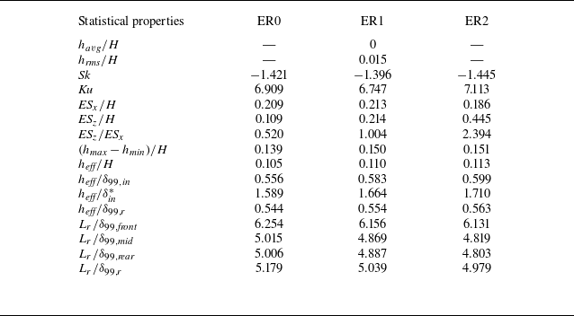
 havg
 hrms
 Sk
 Ku
 ESx
 ESz
 hmax
 hmin
 heff
 δ99,in
 0.99U∞
 δin∗
 δ99,r
 δ99,front
 δ99,mid
 δ99,rear
 Lr
 Re=600
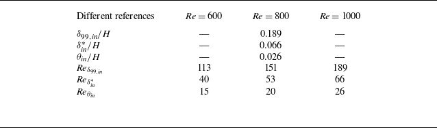
 θin


 x
 z
 z
 y
 y=0.16
 x=5
 Re=1000

 ∑i=19Ii

 Re=1000
 I1
 I2
 I3
 y
 z

 y
 z
 Lx=14, Re=600
 Lx=7, Re=600
 Lx=4, Re=600
 Lx=14, Re=1000
 Lx=4, Re=1000
 Re
 v_I
 v_II
 x:y:z=1:2:3

 σ
 α
 x

 x=9
 α=3,4
 α=4

 t=0
 τopt=5
 α=3
 α=4
 u′
 v′
 w′

 t=0
 τopt,max
 α=4

 †

 ω=0
 x:y:z=1:2:3

 x:y:z=1:2:3

 z=1.5

 x
 x/H=7,9,11,13

 x
 x/H=7,9,11,13

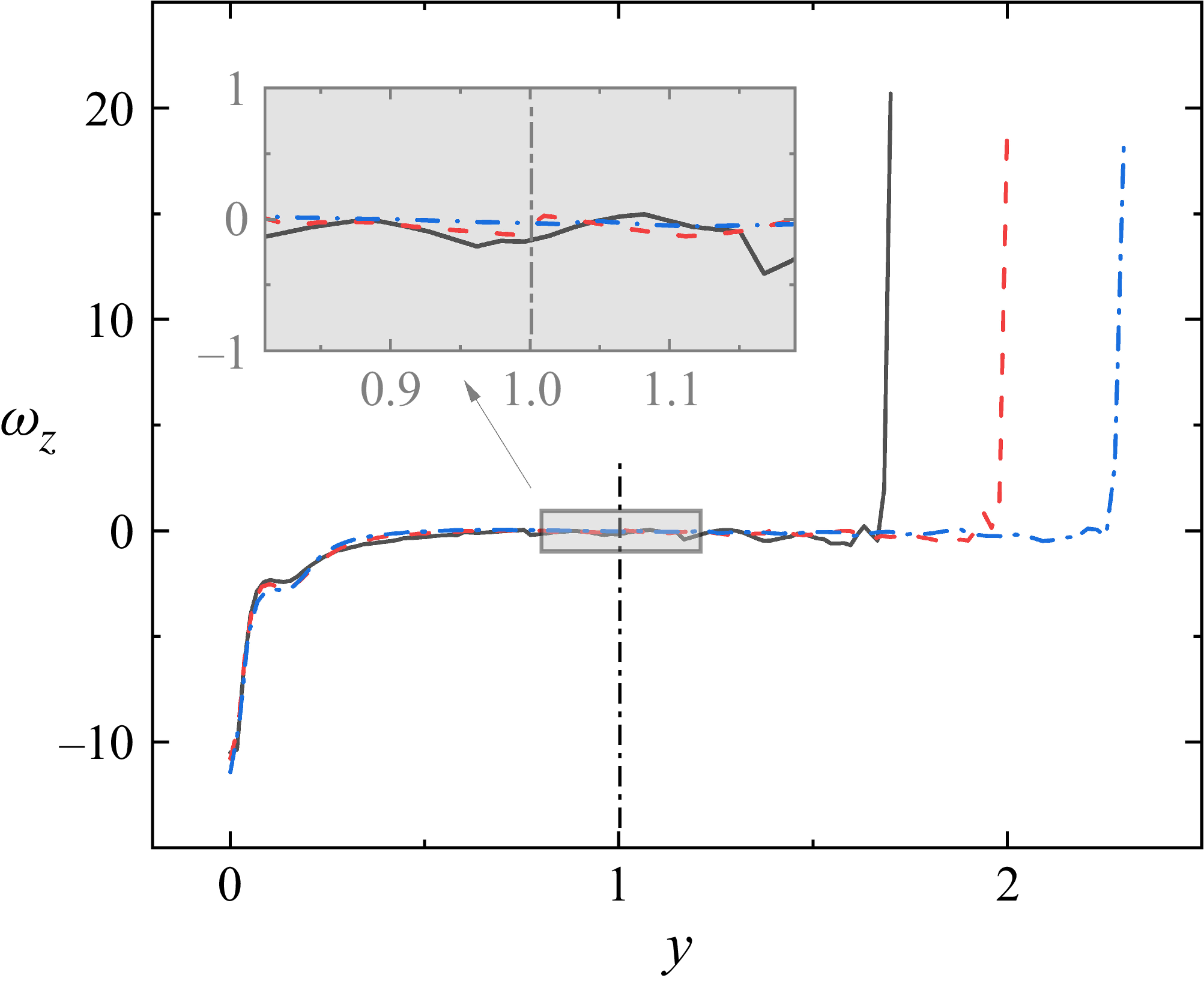
 ymax=1.7
 ymax=2
 ymax=2.3
 x∈[2,10]


