1. Introduction
Characterising flow through heterogeneous porous rocks remains a major challenge for modelling contaminant dispersion in aquifers, the pathways followed by  $\textrm {CO}_2$ during sequestration in subsurface aquifers and the dispersion of chemicals which are injected into oil fields for enhanced recovery. In many sedimentary deposits, the sediment has bedding planes characterised by two values of permeability, parallel and normal to the direction of deposition. Owing to the time dependence of sedimentation processes, especially in fluvial and shallow marine settings, such deposits tend to be highly layered, with the direction of the bedding and of the interface between layers often being in different directions (Allen (Reference Allen1963), see figure 1). For example, Davis et al. (Reference Davis, Lohmann, Phillips, Wilson and Love1993) found that in the Sierra Ladrones formation, there were laterally extensive layers, over 100 m long but only 1–2 m deep, composed of a series of cross-bedded rock elements, with different orientations and anisotropy. Since the scale of the individual rock elements with different properties is typically large compared to the pore scale, the flow through each layer may be described as a continuum, as governed by Darcy's law and the continuity equation, but the development of an upscaled model for the flow through a series of such cross-bedded layers with different orientations is challenging (Dagan Reference Dagan1979). There are models to predict the effective permeability of such formations (Goggin et al. Reference Goggin, Chandler, Kocurek and Lake1988; Tidwell & Wilson Reference Tidwell and Wilson2000) and in reservoir simulation, models often use effective vertical and horizontal permeabilities (Begg & King Reference Begg and King1985; Durlofsky Reference Durlofsky1991; Pickup et al. Reference Pickup, Ringrose, Corbett, Jensen and Sorbie1995; Nordahl & Ringrose Reference Nordahl and Ringrose2008).
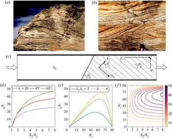
(a,b) Photographs of cross-bedding in Tabernas basin, Spain. (c) A schematic of the model set-up in our idealised problem. Within the cross-bedded layer to the right of the interface, the permeability is  $k_2$ and
 $k_1$, along and across the bedding, and the bedding planes are inclined at an angle
 $\theta _i$ to the lateral boundaries. The interface between the two individual zones of rock is tilted at an angle
 $\theta _e$ to the lateral impermeable boundaries. The interface at
 $z=0.5$ is centred at
 $x=x_c$. The downstream pressure gradient,
 $p_x$ and
 $p_z$, required to maintain uniform flow downstream of the interface, acts at a direction
 $\theta _p$ relative to the lateral impermeable boundaries (1.2). (d,e) The variation of the direction of the downstream pressure gradient,
 $\theta _p$, as a function of (d) the permeability ratio,
 $k_2/k_1$, and (e) the angle of the bedding planes,
 $\theta _i$. (f)Contours of
 $\theta _p$ as a function of thepermeability ratio,
 $k_2/k_1$, and (e) the angle of the bedding planes,
 $\theta _i$.

In a vertically confined but laterally extensive layer of cross-bedded rock, with permeability  $k_1$ and
 $k_2$ in the directions
 $\theta _i$ and
 ${\rm \pi} /2 -\theta _i$ relative to the boundaries, the effective permeability parallel to the boundaries is (figure 1c)
 \begin{equation} \bar{k} = \frac{k_1k_2}{k_1 \sin^2\theta_i + k_2 \cos^2\theta_i}. \end{equation}
In order to maintain a flow parallel to the boundaries, there needs to be a pressure gradient in both vertical and horizontal directions. The net direction of this pressure gradient relative to the boundaries,  $\theta _p$, is given by (cf. Woods (Reference Woods2015))
 \begin{equation} \theta_p = \tan^{{-}1}\left(\frac{p_z}{p_x}\right) \quad \text{where} \ \frac{p_z}{p_x} = \frac{(k_2/k_1-1)\sin\theta_i\cos\theta_i}{\sin^2\theta_i + (k_2/k_1) \cos^2\theta_i}. \end{equation}
This angle of deviation of the pressure gradient is shown in figures 1(d) and 1(e) as a function of the permeability ratio,  $k_2/k_1$, and the direction of the bedding planes relative to the boundary,
 $\theta _i$. It is seen the pressure gradient is tilted towards the direction of lower permeability, and that this tilt depends on the inclination of the bedding and increases with the permeability ratio of this bedding,
 $k_2/k_1$.
In a typical flow channel within a formation, there may be several elements of rock with different orientation or magnitude of the cross-bedding, and with inclined boundaries relative to the flow direction (figure 1a,b). In such formations, we may expect cross-bedding angles to range from  $+45^\circ$ to
 $-45^\circ$ (Pickup et al. Reference Pickup, Ringrose, Corbett, Jensen and Sorbie1995; Klise, Tidwell & McKenna Reference Klise, Tidwell and McKenna2008) and the width of the layers may range from thicknesses of few tens of centimetres to several metres (Davis et al. Reference Davis, Lohmann, Phillips, Wilson and Love1993; Castle et al. Reference Castle, Molz, Lu and Dinwiddie2004), while the length of individual cross-bedding zones may be tens of centimetres to tens of metres (Pickup et al. Reference Pickup, Ringrose, Corbett, Jensen and Sorbie1995). The ratio of
 $k_2/k_1$ in some outcrops was found to vary between 1.6 and 3.5 (Hartkamp, Arribas & Tortosa Reference Hartkamp, Arribas and Tortosa1993; Pickup etal. Reference Pickup, Ringrose, Corbett, Jensen and Sorbie1995). The associated change in the direction and magnitude of the pressure gradient in moving from one element to another can lead to significant distortion of the streamlines, as observed in some laboratory experiments reported by Klise et al. (Reference Klise, Tidwell and McKenna2008). Other efforts to characterise the controls on the flow due to the presence of cross-bedding include the numerical works of Dawe, Caruana & Grattoni (Reference Dawe, Caruana and Grattoni2011) and Sawyer & Cardenas (Reference Sawyer and Cardenas2009), and the field analyses of Huysmans et al. (Reference Huysmans, Peeters, Moermans and Dassargues2008) and Castle et al. (Reference Castle, Molz, Lu and Dinwiddie2004). There has been some stochastic modelling of the role of the interfaces on the distortion of streamlines by using a model with different correlation lengths in the vertical and horizontal directions (Desbarats Reference Desbarats1989; Deutsch Reference Deutsch1989; Corbett & Jensen Reference Corbett and Jensen1992), but there is an incomplete understanding of the basic controls on the dispersion of tracer moving through such a formation.
In this paper we explore the structure of the cross-layer shear which develops in a confined channel as a result of the distortion of the flow when passing (i) through an inclined interface between two isotropic elements of rock of different permeability (§ 2); and (ii) from an isotropic to an anisotropic element of rock, with a vertical boundary between the two layers (§ 3). We then combine these results, to provide new understanding of the shear flow which typically develops in such composite layers (§§ 4 and 5). Recognition of this cross-layer shear is key for prediction of pollutant dispersal and for modelling the dispersion of a pulse of chemical treatment fluid often injected into such reservoirs.
To illustrate the different flow patterns and predict the shear, we use a numerical solution based on flow in a long thin channel, as shown in figure 1(c). For a single phase, incompressible flow through a porous medium, the flow field is given by the continuity equation and Darcy's law. This gives an equation for the velocity field,  $\boldsymbol {u}=(u,v)$, and pressure field,
 $p(x,z)$.
 \begin{equation} \boldsymbol{\nabla} \boldsymbol{\cdot} \boldsymbol{u} = 0 \quad \text{and} \quad \boldsymbol{u} \equiv \begin{pmatrix} u \\ w \end{pmatrix} ={-}\frac{1}{\mu} \begin{pmatrix} k_{xx} & k_{xz} \\ k_{zx} & k_{zz} \end{pmatrix} \begin{pmatrix} \partial p /\partial x \\ \partial p /\partial z \end{pmatrix},\end{equation}
where  $\mu$ is the dynamic viscosity of the fluid, and the components of the permeability tensor are (Bear Reference Bear1971)
 \begin{equation} \left. \begin{array}{c@{}} k_{xx} = K_1 \cos^2\theta_i + K_2 \sin^2\theta_i, \quad k_{zz} = K_2 \cos^2\theta_i + K_1 \sin^2\theta_i,\\ k_{xz} = k_{zx} = (K_1-K_2) \cos\theta_i \sin\theta_i, \end{array}\right\} \end{equation}
where  $K_1=k_0$ and
 $K_2=k_0$ in the isotropic layer and
 $K_1=k_1$ and
 $K_2=k_2$ in the cross-bedded layer.
Equation (1.3a,b) is solved using a pseudo-spectral code in Dedalus (Burns et al. Reference Burns, Vasil, Oishi, Lecoanet and Brown2019). We use Fourier modes in the along-channel ( $x$) direction and Chebyshev modes in the cross-channel (
 $z$) direction. We use an iteration scheme to converge to the solution for the pressure. We use
 $2048$ and
 $512$ spectral modes in the
 $x$ and
 $z$ directions respectively to resolve the permeability field. We assume the solution has converged when the residual defined as
 \begin{equation} \mathcal{R} = \int_V \vert \boldsymbol{\nabla} \boldsymbol{\cdot} \boldsymbol{u} \vert \,\mathrm{d}V \end{equation}
has asymptoted to a constant value, which is always smaller than  $10^{-4}$ of its initial value. We have then tested the sensitivity of the model predictions to the number of modes in the representation of the solution. We find that the difference between solutions when using
 $(4096, 1024)$ modes and
 $(2048,512)$ modes is less than 0.05 %.
Using the computed pressure field, we calculate the flow field using Darcy's equation (1.3a,b). If the interface is centred at along-channel position  $x_c$, then to estimate the travel times along individual streamlines,
 $t_s$, over the region
 $(x_c-L/2)< x < (x_c+L/2)$, we integrate along each streamline
 \begin{equation} t_s(z,L) = \int_{x_c-L/2}^{x_c+L/2} \frac{\mathrm{d}x}{u_s(x,z)}. \end{equation}
Here,  $u_s$ is the horizontal component of speed of the fluid along individual streamlines, and
 $z$ is the height of the streamline above the lower boundary of the flow channel in the region of parallel flow far downstream of the interface. Variations in
 $t_s$ as a function of
 $z$ lead to an effective shear which has a leading-order impact on the dispersal of material being carried with the flow. Across all simulations, we keep the channel dimensions (
 $0 \leq x\leq D$ and
 $0\leq z \leq H=1$) and the location of the centre of the interface constant
 $(x_c=5, z_c= 0.5)$ and we set
 $L=D/2$.
In the next sections, we work with dimensionless variables, with the vertical scale representing the vertical extent of a laterally extensive layer of cross-bedded rock which is bounded above and below by an impermeable seal rock. The horizontal scales are referenced relative to this vertical scale. Depending on the application and the geological setting of the formation, the vertical scale may range from tens of centimetres to several metres.
2. Shear generation across a tilted interface in a confined channel
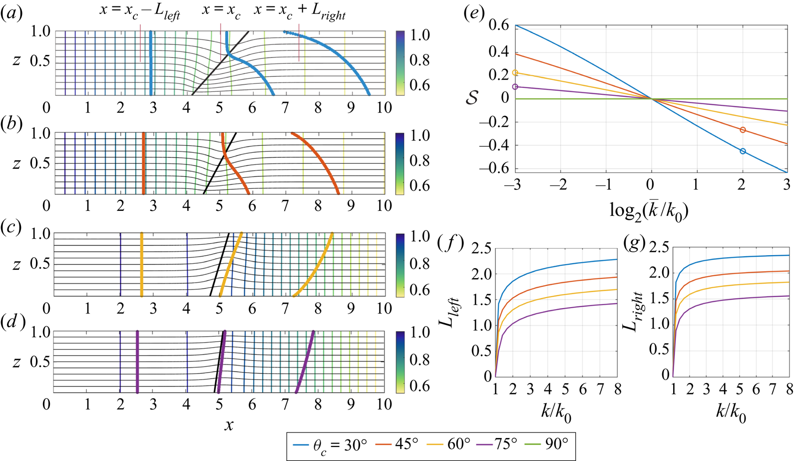
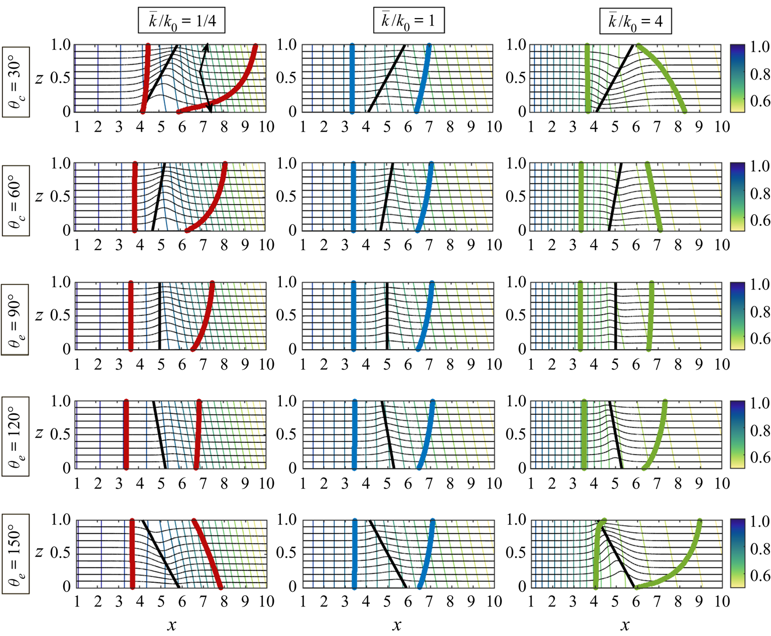
If the interface between two isotropic layers of different permeability, which are confined between two impermeable parallel boundaries, is tilted relative to the boundaries, then a transition zone develops across which the pressure gradient adjusts from the upstream to the downstream value. In figures 2(a)–2(d) this may be seen both in terms of the distortion to the streamlines (thin black curves), the distortion to the surfaces of constant pressure near the interface (thin coloured lines), and also the motion of a streak of dye (thick line). The interface is shown with a thick black line; a similar graphical scheme is used for all subsequent plots illustrating the flow in this paper.
(a)–(d) The thick black line shows the interface between two isotropic zones of rock with permeability  $k_0$ to the left and
 $\bar {k}$ to the right. The thin coloured lines indicate contours of constant pressure,
 $p(x,z)$, and the thin black curves show the streamlines of the flow. The thick coloured lines show the location of a line of tracer at three times after the initial release at
 $x=0$ and
 $t=0$ (in blue, orange, yellow and purple respectively). In panels (a,b),
 $\bar {k}=4$,
 $k_0=1$. In panels (c,d),
 $\bar {k}=1/8$,
 $k_0=1$. (e) The shear strength,
 $\mathcal {S}$, is shown as a function of the permeability ratio,
 $\bar {k}/k_0$, with the results for panels (a)–(d) labelled on this figure. (f,g) The transition distances from uniform flow upstream of the interface,
 $L_{left}$, to uniform flow downstream of the interface,
 $L_{right}$, are shown as a function of the permeability ratio,
 $\bar {k}/k_0$ (see panel a). In all panels, the colours correspond to the angle of the interface,
 $\theta _e$.

In panels (a,b), the region to the right of the interface has the higher permeability,  $\bar {k}=4k_0$. Streamlines at the base of the channel therefore reach the higher permeability zone sooner, and so have a shorter travel time through the domain. In turn, the streaks of dye released into the flow upstream, as shown by the (a) blue and (b) orange lines, become sheared out towards the base of the layer. In figures 2(c) and 2(d), the region to the right has a lower permeability, and so along the streamlines at the base of the channel, the flow slows down on passing through the interface. Thus, at the base of the channel, the streak of dye lags that higher in the formation, leading to a shear in the opposite sense to panels (a,b).
The strength of the shear generated in the transition zone depends on the permeability contrast and the angle of inclination of the interface. To quantify this shear, we first define the transition zone as being the region  $x_c-L_{left} < x < x_c+L_{right}$, in which the horizontal velocity,
 $u(x,z)$, at some point across the channel deviates by more than
 $0.5 \%$ of the uniform far-field flow (see figure 2a), where
 $x_c$ is at the centre of the interface. Figures 2(f) and 2(g) show the variation of the size of the transition zone as a function of the permeability ratio between the two regions,
 $\bar {k}/k_0$, for a range of angles of inclination of the interface. We then estimate the travel times,
 $t_a(z)$, along individual streamlines at each height
 $z$ in the layer by integrating along each streamline in the region,
 $(x_c-L/2)< x < (x_c+L/2)$, where the interface is centred at along-channel position
 $x=x_c$ and where (
 $L>2\max (L_{left},L_{right})$). We repeat similar calculations for all permeability ratios and interface angles considered in this paper. Note also that in all our calculations, we integrate over a region of length
 $L=5$ since this always exceeds the length of the transition zone for the choice of parameters shown in this paper.
We can define a dimensionless shear strength,  $\mathcal {S}$, as
 \begin{equation} \mathcal{S} = \frac{U(z=H)-U(z=0)}{\bar{U}}, \quad \text{where} \ U(z) = \frac{L}{t_a(z)} \quad \text{and} \quad \bar{U} = \frac{1}{H}{\int_0^H U(z)}, \end{equation}
where  $H$ is the channel width. Figure 2(e) shows this shear strength as a function of the permeability contrast across the interface for interfaces with angles of tilt
 $\theta _e=30^\circ$,
 $45^\circ$,
 $60^\circ$,
 $75^\circ$ and
 $90^\circ$. Note that the shear has the same size but changes sign under the mapping
 $k_1/k_2 \to k_2/k_1$.
3. Shear production at a vertical interface with an anisotropic layer
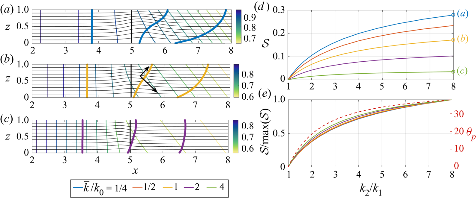
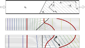
When the region downstream of the interface is cross-bedded, the pressure gradient associated with the uniform flow downstream is directed at an angle to the boundaries, as seen by the contours of constant pressure in figures 3(a)–3(c) (cf. figure 1d,e). The pressure gradient tilts towards the direction of the lower permeability in the cross-bedded zone, as shown by the shorter black arrow in panel (b). This leads to a weakening of the pressure gradient at the base of the interface which results in the development of a net shear in the transport of the tracer (blue, yellow and green lines) across the interface zone since the flow is weaker near the base than at the top of the zone. The calculations in figures 3(a)–3(c) correspond to a bedding angle of  $45^\circ$ and a permeability contrast within the cross-bedded layer of 1 : 8.
(a–c) Streamlines (thin black curves), pressure contours (thin coloured lines) and tracer location (in thick blue, yellow and green lines respectively) at three times after the initial release, for the flow through a porous layer in which the region  $x<5$ is isotropic with permeability
 $k_0=1$, and the region
 $x>5$ is cross-bedded with the permeability ratio across and along the layers,
 $k_2/k_1 = 8$. In these calculations,
 $\theta _i=45^\circ$ as indicated by the black arrows in panel (b). (d) Variation of the shear strength,
 $\mathcal {S}$, as a function of
 $k_2/k_1$, for five values of the effective along-layer permeability of the cross-bedded zone,
 $\bar {k}/k_0$. (e) The normalised shear strength,
 $\mathcal {S}/\max (\mathcal {S})$ (solid lines), and the direction of the downstream pressure gradient in the cross-bedded region (dotted line, cf. figure 1d), as a function of the permeability ratio,
 $k_2/k_1$.

Figures 3(a)–3(c) illustrate the dependence of the shear on the effective horizontal permeability change across the interface. With a decrease in effective along-layer permeability from 1 to 0.25 (panel a), the pressure gradient becomes larger downstream and this amplifies the difference in the speed between the top and the base of the layer near the interface, as may be seen by the deformation of the streamlines. As a result a significant shear develops. When the effective permeability downstream equals that upstream (panelb), a significant shear still develops owing to the change in direction of the pressure gradient, although the shear is weaker. When the effective along-layer permeability is 4 times larger than that upstream (panel c), the pressure gradient becomes weaker downstream of the interface and this reduces the difference in the flow speed between the top and base of the interface, as may be seen by the much smaller deformation of the streamlines, thereby leading to a much smaller shearing of the tracer as it passes through the interface.
In figure 3(d) we illustrate the change in the magnitude of the shear as the permeability contrast in the cross-bedded layer,  $k_2/k_1$, changes. These calculations were made while keeping the mean permeability constant in the cross-bedded region; the closer the internal permeability ratio of the cross-bedded region,
 $k_2/k_1$, is to unity, the smaller the shear (cf. figure 1d). On rescaling the shear with its maximum value, the curves in panel(d) appear to collapse (panel e), and the trend follows the increase in magnitude of the direction of the pressure gradient relative to the boundary,
 $\theta _p$, as
 $k_2/k_1$ increases, as shown by the dashed line (cf. figure 1d).
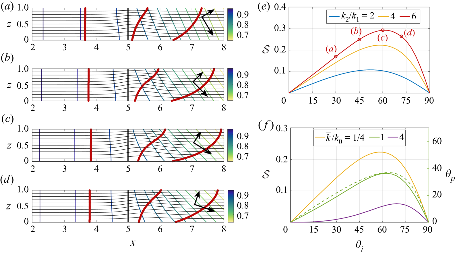
The above calculations focus on the case that the cross-bedded region has bedding plane of  $45^\circ$. If the orientation of the bedding planes change, then the direction of the downstream pressure gradient will also change (figure 1e) and in turn this will impact the shear. In figures 4(a)–4(d), we illustrate the change in the shear, as illustrated by the distortion of the line of tracer on passing through an interface into a cross-bedded region, when the orientation of the bedding planes changes from
 $30^\circ$ to
 $72^\circ$. The black arrows show the direction of the permeability in each case. Figure 4(d) illustrates the variation of the shear with angle
 $\theta _i$ for three values of
 $k_2/k_1$; the red curve corresponds to panels (a)–(d). As the permeability ratio,
 $k_2/k_1$, decreases towards unity (yellow and blue lines) with an effective permeability of the downstream layer,
 $\bar {k} = k_0/4$, the shear also decreases. For a given permeability ratio in the cross-bedded region,
 $k_2/k_1$, then as the direction of the bedding plane
 $\theta _i$ changes, the magnitude of the shear follows the magnitude of the direction of the pressure gradient relative to the boundaries,
 $\theta _p$, as may be seen by comparing the solid and dashed green lines in figure 4(f) (cf. figure 1e). This figure also illustrates that the magnitude of the shear increases as the effective permeability of the cross-bedded region in the along-layer direction becomes smaller.
(a–d) Streamlines (thin black curves), pressure contours (thin coloured lines) and tracer locations (thick red lines) at three times after the initial release at  $x = 2$ and
 $t = 0$ into a porous layer with isotropic permeability for
 $x<5$ and which is cross-bedded for
 $x>5$, with the ratio of permeability along and across the beds
 $k_2/k_1= 6$. The cross-bedding is oriented at angles
 $\theta _i=30^\circ$ (a),
 $45^\circ$ (b),
 $60^\circ$ (c) and
 $72^\circ$ (d), as indicated by the thick arrows on each panel. (e,f) Variation of the shear strength,
 $\mathcal {S}$, as a function of the angle of cross-bedding,
 $\theta _i$, for different values of (e)
 $k_2/k_1$, with
 $\bar {k}/k_0=1/4$, and (f)
 $\bar {k}/k_0$ with
 $k_2/k_1=4$. The shear strength for the flow realisations in panels (a)–(d) are shown in panel (e). The dotted line in panel (f) corresponds to the direction of the downstream pressure gradient in the cross-bedded region (cf. figure 1e) for
 $k_2/k_1=4$ and
 $\bar {k}/k_0=1$.

4. Shear generation in anisotropic layers with a tilted interface
We now explore the interaction between the two different mechanisms of generating shear: shear production at an inclined interface between two zones of different permeability (§ 2) and shear production at an interface between an isotropic and a cross-bedded layer (§ 3). In figure 5, we illustrate the change in flow pattern as the tilt of the interface at a boundary between an isotropic and a cross-bedded layer is changed, for three values of the effective permeability in the cross-bedded layer relative to the isotropic layer.
In all panels, the region to the left of the interface, indicated with a solid black line, is isotropic with permeability  $k_0$ and the region to the right is cross-bedded, with the bedding permeability ratio
 $k_2/k_1=4$ and angle of bedding
 $\theta _i=45^\circ$ as indicated by the arrows in the top left panel. Each row and column corresponds to a different value of mean permeability,
 $\bar {k}/k_0$, for the cross-bedded region, and a different angle of the interface,
 $\theta _e$, as indicated. Streamlines are shown with the thin black curves, pressure contours with the thin coloured lines, the location of line of tracer at two times is shown with a thick coloured line.

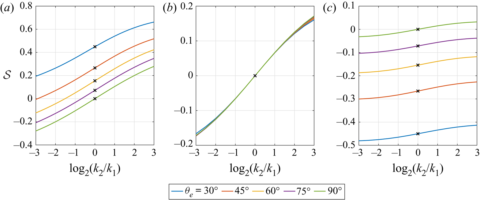
For reference, the central row of panels, with a vertical interface as indicated by the solid black line, illustrates the difference between an anisotropic layer with a small effective permeability (left) and with a high effective permeability (right). In the low permeability case, tilting the interface in the direction of the pressure gradient (upper two panels, left-hand side) increases the shear since the effect of the tilted interface combines with the effect of the anisotropy. Tilting the interface in the opposite sense leads to a reduction in the shear and eventually a reversal as the tilt dominates the effect of the cross-bedding (lower left-hand panels). In contrast, with a more permeable cross-bedded layer, the shear is quite small when the interface is vertical (middle right-hand panel; cf. figure 3). Since the pressure gradient is weaker downstream, then tilting the interface causes the direction of the pressure gradient to tilt in the opposite sense as the tilt of the interface. If tilt of the interface is in the same sense as the direction of the pressure gradient downstream, then the interface counteracts the effect of the cross-bedding (top right-hand panels), and eventually can lead to an overall reversal of the sense of the shear. If the interface tilt is opposite to the direction of the pressure gradient in the cross-bedded layer (lower right-hand panels), the effect of the tilt now combines with the cross-bedding to enhance the shear. The middle column of panels in figure 5 shows that if the effective permeability in the downstream cross-bedded element,  $\bar k$, is the same as that upstream then the shear is relatively small, and is little affected by the tilt of the interface; it is primarily dominated by the adjustment of the flow since the direction of the pressure gradient is not parallel to the boundaries in the cross-bedded layer far downstream.
Figure 6 summarises these results, and also illustrates the sensitivity of the shear to the permeability ratio in the cross-bedded zone, with the shear being enhanced by a larger permeability ratio as expected from figure 3. Also, the figure illustrates how the shear depends on the orientation of the interface, with the different lines corresponding to different interface orientations. Indeed, the shear can reverse in sign when interface-induced shear dominates, as already noted in figure 5. Figure 6(b) also shows the insensitivity of the shear to the angle of tilt in the case that the effective permeability downstream matches that in the isotropic layer upstream (cf. the middle column of panels in figure 5).
The shear strength,  $\mathcal {S}$, is shown as a function of the strength of the permeability ratio across the cross-bedding,
 $k_2/k_1$, with
 $\bar {k}/k_0=1/4$ (a),
 $1$ (b) and
 $4$ (c). The colours correspond to the angle of the interface with the isotropic layer upstream,
 $\theta _e=30^\circ$,
 $45^\circ$,
 $60^\circ$,
 $75^\circ$ and
 $90^\circ$. In all calculations,
 $\theta _i=45^\circ$. The black crosses indicate isotropic blocks with
 $k_2=k_1$.

5. Discussion
We find that in a composite permeable rock, bounded above and below by impermeable boundaries, and composed of discrete zones of permeable rock, the adjustment of the flow from one zone to the next can lead to distortion of the flow and the generation of a net vertical shear in the averaged flow through the formation. This shear arises from a combination of the inclination of the interface between adjacent zones of rock with different permeability, and also from the change in direction of the pressure gradient as the flow moves from one zone to another, since in cross-bedded layers, the pressure gradient is typically not aligned with the direction of the flow (figure 1). We have demonstrated how these two different effects may interact and compete, thereby enhancing or reducing the magnitude and the sense of the shear.
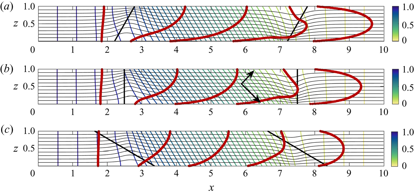
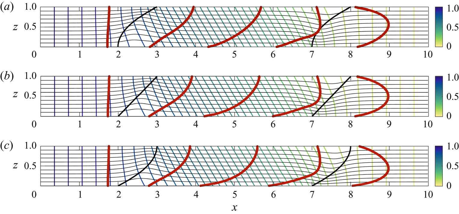
In the models presented in this paper we focus on a single interface to expose the fundamental controls, but in a composite rock, there will likely be multiple zones of rock with multiple associated interfaces. Since the shear associated with each interface typically exhibits a curvature, so that the shear becomes stronger nearer the slower part of the velocity profile (figures 2–5), then on averaging the flow across multiple interfaces, this is likely to lead to a more symmetrical velocity profile, with a maximum speed near the centre of the channel. Although there are many more calculations which can be carried out, as one simple illustration of this effect we consider the net shear which arises when a finite trapezoid shaped element of cross-bedded material with parallel interfaces is embedded in a uniform porous layer, as shown in figures 7(a)–7(c). When the interfaces are sufficiently far apart, the transition zone of the pressure gradient for the two interfaces are independent, and the shear associated with each interface are additive. Since the second interface produces a shear which is the mirror image of the first interface, the net effect is a symmetrical velocity profile downstream; as with the earlier results in the paper, the tilted interface may enhance (panel a) or reduce (panel c) the shear associated with the cross-bedding (panel b). In figure 8, we illustrate the impact of a curvature in the interface between two layers of rock on the distortion of the tracer. The distortion is of a similar magnitude to the linear interface case (panel b). However, as may be seen in the flow downstream of the cross-bedded zone, the curvature of the interface does lead to a small asymmetry in the ultimate tracer profile downstream (panels a,c).
Streamlines (thin black curves), pressure contours (thin coloured lines) and tracer locations (thick red lines) at five times after release from  $x=0$. The porous layer consists of an isotropic rock of permeability
 $k_0$, while the central trapezoidal region of length
 $d=5$ is a cross-bedded zone with permeability ratio across the bedding planes
 $k_2/k_1=4$, and mean effective permeability along the layer
 $\bar {k}/k_0=1/4$. The angle of the bedding is
 $\theta _i=45^\circ$, and the direction of permeability within this region is indicated by the arrows in panel (b). Panels (a)–(c) correspond to interface angle
 $\theta _e=60^\circ ,\;90^\circ ,\;150^\circ$ respectively (cf. figure 5).

Streamlines (thin black curves), pressure contours (thin coloured lines) and tracer locations (thick red lines) at three times after release from  $x=0$. The porous layer consists of an isotropic rock of permeability
 $k_0$ within which there is a cross-bedded zone with permeability ratio across the bedding planes
 $k_2/k_1=4$ and mean effective permeability along the layer
 $\bar {k}/k_0=1/2$. The angle of the bedding is
 $\theta _i=45^\circ$, and the direction of permeability within this region is indicated by the arrows in panel (b). In panel (b), the interface angle is linear, with angle
 $\theta _e=45^\circ$, while panels (a,c) correspond to a parabolic interface with opposite curvatures.

The present results identify that in composite cross-bedded formations, bounded by impermeable rock, the flow can develop a strong shear. In the models presented in this paper, we explore the shearing of a pulse of dye which results from the mean velocity profile; if a field-scale test of tracer dispersion is carried out, such shear will act to spread the arrival time of the tracer at this point, and hence will have a leading-order effect on the results. The use of simplified ‘effective permeability’ values in the direction of the flow for simulation of the transport of tracer, or of a fluid–fluid interface, neglects the effects of shear, which is central for predicting the dispersion and stretching of the flow within this type of bounded porous layer. There are many possible developments of this work exploring the shear which develops at the interface between different zones of permeable rock. For example, if there is a temperature gradient across the rock, this will lead to changes in density and viscosity of the fluid, further influencing the pattern of shear as tracer moves with the flow; we are presently exploring some of these processes.
Declaration of interests
The authors report no conflict of interest.