1 Introduction
The skin friction exerted by turbulence causes significant energy losses in flow systems, and thus reduction of the skin friction in a turbulent boundary layer is one of the most important and challenging problems in fluid mechanics. Various control methods have been suggested to reduce the skin friction (Kim Reference Kim2003, Reference Kim2011; Collis et al.
Reference Collis, Joslin, Seifert and Theofilis2004). Among these control methods, active ones have the potential to achieve the control purpose, and can be categorized into feedback and feedforward ones depending on the usage of sensors for feedback. Examples of feedforward controls (i.e. without sensors for feedback) are spanwise wall oscillation (Jung, Mangiavacchi & Akhavan Reference Jung, Mangiavacchi and Akhavan1992; Quadrio & Ricco Reference Quadrio and Ricco2004), streamwise-travelling waves of blowing and suction (Min et al.
Reference Min, Kang, Speyer and Kim2006) and wall deformation (Nakanishi, Mamori & Fukagata Reference Nakanishi, Mamori and Fukagata2012), and streamwise-travelling waves of spanwise velocities (Quadrio, Ricco & Viotti Reference Quadrio, Ricco and Viotti2009). These control methods have been implemented in experiments (see, e.g., Choi, DeBisschop & Clayton Reference Choi, DeBisschop and Clayton1998; Choi, Jukes & Whalley Reference Choi, Jukes and Whalley2011) and have shown large amounts of drag reduction. However, they require relatively large power inputs to provide the control input, such as the oscillating wall. On the other hand, feedback controls are expected to be more efficient than feedforward ones. A well-known example of a feedback control is the opposition control suggested by Choi, Moin & Kim (Reference Choi, Moin and Kim1994). This control method provided blowing and suction at the wall that was opposite to the instantaneous wall-normal velocity at the sensing plane above the wall. The effect of the sensing plane location (
 $y_{s_{0}}^{+}=y_{s}u_{\unicode[STIX]{x1D70F}_{0}}/\unicode[STIX]{x1D708}$
) on the skin-friction reduction was investigated, from which
 $y_{s_{0}}^{+}\approx 10$
was provided to be the optimal location for the skin-friction reduction (approximately 25 %), where
 $u_{\unicode[STIX]{x1D70F}_{0}}$
is the wall-shear velocity of uncontrolled flow and
 $\unicode[STIX]{x1D708}$
is the kinematic viscosity. Later, Hammond, Bewley & Moin (Reference Hammond, Bewley and Moin1998) reported that a sensing plane of
 $y_{s_{0}}^{+}=15$
resulted in a slightly larger skin-friction reduction. Chung & Talha (Reference Chung and Talha2011) investigated the effects of the amplitude of blowing and suction, and showed that the optimal location of the sensing plane depends on the amplitude of blowing and suction. The applicability of opposition control to higher Reynolds numbers has been also investigated by other researchers (Chang, Collis & Ramakrishnan Reference Chang, Collis and Ramakrishnan2002; Iwamoto, Suzuki & Kasagi Reference Iwamoto, Suzuki and Kasagi2002; Pamiés et al.
Reference Pamiés, Garnier, Merlen and Sagaut2007). However, opposition control has practical difficulties in implementing sensors at a sensing plane located very near the wall, and thus control methods with sensors at the wall were introduced for more practical purposes (Choi et al.
Reference Choi, Moin and Kim1994; Lee et al.
Reference Lee, Kim, Babcock and Goodman1997; Lee, Kim & Choi Reference Lee, Kim and Choi1998; Lee et al.
Reference Lee, Cortelezzi, Kim and Speyer2001). In the latter two studies, the blowing and suction was determined by the weighted average of neighbouring wall-shear stresses or wall pressures. These feedback controls are much harder to implement in experiments than feedforward ones, but some experiments have been performed to realize these feedback controls using distributed microsensors and actuators (Kasagi, Suzuki & Fukagata Reference Kasagi, Suzuki and Fukagata2009).
More systematic methods based on control theories have been also suggested for skin-friction reduction or the reduction of transient growth of disturbances. For example, gradient-based optimal and suboptimal controls were proposed by Abergel & Temam (Reference Abergel and Temam1990), Choi et al. (Reference Choi, Temam, Moin and Kim1993) and Bewley & Moin (Reference Bewley, Moin, Wang, Von Flotow, Shoureshi, Hendricks and Farabee1994), and
 ${\mathcal{H}}_{\infty }$
(robust) and
 ${\mathcal{H}}_{2}$
(optimal) controls were suggested by Bewley & Liu (Reference Bewley and Liu1998), Joshi, Speyer & Kim (Reference Joshi, Speyer and Kim1999), Lee et al. (Reference Lee, Cortelezzi, Kim and Speyer2001), Högberg, Bewley & Henningson (Reference Högberg, Bewley and Henningson2003), Chevalier et al. (Reference Chevalier, Hœpffner, Åkervik and Henningson2007), Sharma et al. (Reference Sharma, Morrison, Mckeon, Limebeer, Koberg and Sherwin2011) and Nita, Vandewalle & Meyers (Reference Nita, Vandewalle and Meyers2016). Although these controls were successful in achieving their goals, they require more information on flow fields or somewhat excessive computational work, making it difficult for them to be implemented for the control of turbulent flow.
One of the most popular linear controls in the control society is proportional (P)–integral (I)–differential (D) control. Proportional–integral–differential control has been used widely for engineering applications. Because a PID controller determines the actuation directly from the sensing variable without additional computations, it may be easily implemented in flow systems. Nevertheless, PID control has been applied to only a few fluid flows, including flow over a cylinder and flow with two-dimensional perturbations in a channel. Since the purpose of the present study is skin-friction reduction, we do not discuss the flow over a cylinder in the present paper; for more details on the application of PID control to this flow, see the recent studies by Son, Jeon & Choi (Reference Son, Jeon and Choi2011) and Das et al. (Reference Das, Mathew, Shaiju and Patnaik2016), and references therein. Hu & Bau (Reference Hu and Bau1994) applied P control based on wall-shear measurement to stabilize a laminar plane channel flow by changing the viscosity by heating and cooling at the wall. Joshi, Speyer & Kim (Reference Joshi, Speyer and Kim1997) applied a linear control theory to stabilize the flow in a two-dimensional channel by blowing and suction at the wall with measurement of the wall-shear stress. Opposition control (Choi et al.
Reference Choi, Moin and Kim1994), mentioned above, is also a type of P control with a proportional gain of
 $\unicode[STIX]{x1D6FC}=1$
, and the change in the amplitude of blowing and suction in the work by Chung & Talha (Reference Chung and Talha2011) and Deng et al. (Reference Deng, Xu, Huang and Cui2014) is also a P control with different magnitudes of the proportional gain. According to Son et al. (Reference Son, Jeon and Choi2011), a PID control is considered as a P control with a phase shift if the system under consideration is linear. Therefore, opposition control with upstream sensing (Lee Reference Lee2015) can be considered as a PID control if the near-wall dynamics in turbulent channel flow is assumed to be essentially linear.
To the best of our knowledge, there has been no attempt to apply PI or PID controls to turbulent channel (or boundary layer) flow, although a P control has been applied to this flow, as mentioned above. Therefore, in the present study, we apply PI control to turbulent channel flow for skin-friction reduction, and compare its performance with that of P control. Here, we do not consider the D (differential) component of PID control because the system becomes easily unstable with this component due to turbulent fluctuations in channel flow. We vary the sensing plane location (
 $y_{s_{0}}^{+}$
) and the proportional and integral gains (
 $\unicode[STIX]{x1D6FC}$
and
 $\unicode[STIX]{x1D6FD}$
) to investigate their effects on the performance of skin-friction reduction. To further understand the performance of PI controls, we also consider a linearized flow model having transient growth of disturbances in a channel. Details of the PI control and numerical methods are described in § 2. The results of the PI control for a turbulent channel flow from direct numerical simulations are given in § 3. In § 4, we show the performance of the PI control applied to a flow model obtained from the linearized Navier–Stokes equations, followed by conclusions in § 5.
2 Control method and numerical details
2.1 Proportional–integral–differential control
The linear PID control is based on only the output being available for feedback, and its controller is composed of the simple gain (P control), integrator (I control) and differentiator (D control), or some weighted combination of these components, as follows:
 $$\begin{eqnarray}\unicode[STIX]{x1D713}(t)=\unicode[STIX]{x1D6FC}e(t)+\unicode[STIX]{x1D6FD}\int _{0}^{t}e(\unicode[STIX]{x1D70F})\,\text{d}\unicode[STIX]{x1D70F}+\unicode[STIX]{x1D6FE}\frac{\text{d}e(t)}{\text{d}t}.\end{eqnarray}$$
Here,
 $\unicode[STIX]{x1D713}(t)$
is the control input,
 $e(t)\;(=r(t)-\unicode[STIX]{x1D701}(t))$
denotes the error (that is, the discrepancy between the reference input
 $r(t)$
and the control output
 $\unicode[STIX]{x1D701}(t)$
), and
 $\unicode[STIX]{x1D6FC}$
,
 $\unicode[STIX]{x1D6FD}$
and
 $\unicode[STIX]{x1D6FE}$
are the proportional, integral and differential gains respectively. The proportional part adjusts the output signal in direct proportion to the error. When the proportional gain
 $\unicode[STIX]{x1D6FC}$
increases, the system under consideration yields a fast response, small steady-state errors and a highly oscillatory response. The integral part corrects for any error that may occur between the desired value and the process output over time. Thus, the steady-state error can be zero due to the integral part. However, because the integral part responds to accumulated errors from the past, it can cause the present value to overshoot the set-point value. The differential part uses the rate of change of the error signal and forces the error to zero, without oscillations of excessive amplitude. However, the differential part slows the transient response of the controller and is highly sensitive to noise in a signal, because it amplifies the noise, the high-frequency component of the signal. Thus, the differential part makes a process unstable when the noise and differential gain are sufficiently large. For this reason, we consider only P and PI controls for the present turbulent channel flow. In the present study, the control output
 $\unicode[STIX]{x1D701}(t)$
is the sensing velocity
 $v_{s}$
, which is the wall-normal velocity at a sensing plane above the wall. We set the reference input
 $r(t)$
to zero, meaning that we consider the control output
 $\unicode[STIX]{x1D701}(t)$
itself as an error with opposite sign (
 $e=-\unicode[STIX]{x1D701}$
) and want to drive
 $\unicode[STIX]{x1D701}(t)$
to zero through the present feedback control. A successful feedback control removes the wall-normal velocity fluctuations at the sensing plane, which may in turn reduce the strength of near-wall streamwise vortices and result in a decrease in the skin friction.
2.2 Numerical methods
The governing equations for an unsteady incompressible viscous flow are given as
 $$\begin{eqnarray}\displaystyle & \displaystyle \frac{\unicode[STIX]{x2202}u_{i}}{\unicode[STIX]{x2202}t}+\frac{\unicode[STIX]{x2202}u_{i}u_{j}}{\unicode[STIX]{x2202}x_{j}}=-\frac{\text{d}P}{\text{d}x_{1}}\unicode[STIX]{x1D6FF}_{i1}-\frac{\unicode[STIX]{x2202}p}{\unicode[STIX]{x2202}x_{i}}+\frac{1}{Re}\frac{\unicode[STIX]{x2202}^{2}u_{i}}{\unicode[STIX]{x2202}x_{j}\unicode[STIX]{x2202}x_{j}}, & \displaystyle\end{eqnarray}$$
 $$\begin{eqnarray}\displaystyle & \displaystyle \frac{\unicode[STIX]{x2202}u_{i}}{\unicode[STIX]{x2202}x_{i}}=0, & \displaystyle\end{eqnarray}$$
where the
 $x_{i}$
are the Cartesian coordinates, the
 $u_{i}$
are the corresponding velocity components
 $(u,v,w)$
,
 $p$
is the pressure fluctuation and
 $-\text{d}P/\text{d}x_{1}$
is the mean streamwise pressure gradient to drive a constant mass flow rate in a channel. All variables are non-dimensionalized by the channel half-height (
 $h$
) and laminar centreline velocity (
 $u_{l}=(3/2)u_{b}$
;
 $u_{b}$
is the bulk mean velocity). The Reynolds number considered is
 $Re=u_{l}h/\unicode[STIX]{x1D708}=3000$
(
 $Re_{\unicode[STIX]{x1D70F}}=u_{\unicode[STIX]{x1D70F}_{0}}h/\unicode[STIX]{x1D708}\approx 140$
). The Reynolds number considered here is quite low but is within the range (
 $Re_{\unicode[STIX]{x1D70F}}=100{-}180$
) considered in previous studies (Choi et al.
Reference Choi, Moin and Kim1994; Lee et al.
Reference Lee, Kim, Babcock and Goodman1997, Reference Lee, Kim and Choi1998; Hammond et al.
Reference Hammond, Bewley and Moin1998; Högberg et al.
Reference Högberg, Bewley and Henningson2003; Chung & Talha Reference Chung and Talha2011; Sharma et al.
Reference Sharma, Morrison, Mckeon, Limebeer, Koberg and Sherwin2011; Deng et al.
Reference Deng, Xu, Huang and Cui2014; Lee Reference Lee2015; Nita et al.
Reference Nita, Vandewalle and Meyers2016). Chang et al. (Reference Chang, Collis and Ramakrishnan2002) and Iwamoto et al. (Reference Iwamoto, Suzuki and Kasagi2002) applied P controls to turbulent channel flow at various Reynolds numbers, and showed that the maximum amount of skin-friction reduction and its optimal sensing location (
 $y_{s_{0}}^{+}$
) decrease with increasing Reynolds number. Thus, the results from the present parametric study on the sensing plane (
 $y_{s_{0}}^{+}$
) and feedback gains (
 $\unicode[STIX]{x1D6FC}$
and
 $\unicode[STIX]{x1D6FD}$
) should also be dependent on the Reynolds number, but the main conclusions regarding the effects of these parameters on the skin-friction reduction obtained at low Reynolds number should not be significantly changed even at higher Reynolds number.
A second-order semi-implicit fractional step method is used for time advancement, a third-order Runge–Kutta method is used for convective terms and the Crank–Nicolson method is used for diffusive terms. The second-order central difference scheme is applied to spatial derivative terms. Periodic boundary conditions are used in the streamwise and spanwise directions, and a no-slip condition is applied to both the upper and lower walls (
 $u=w=0$
). The computational domain size is
 $3\unicode[STIX]{x03C0}(x)\times 2(y)\times \unicode[STIX]{x03C0}(z)$
and the number of grid points is
 $64(x)\times 65(y)\times 64(z)$
. Uniform grids are used in the streamwise and spanwise directions, while a non-uniform grid is used in the wall-normal direction. The grid spacings in wall units are
 $\unicode[STIX]{x0394}x_{0}^{+}=\unicode[STIX]{x0394}xu_{\unicode[STIX]{x1D70F}_{0}}/\unicode[STIX]{x1D708}\approx 20$
,
 $\unicode[STIX]{x0394}y_{min\;0}^{+}\approx 0.45$
,
 $\unicode[STIX]{x0394}z_{0}^{+}\approx 6.6$
respectively, which are slightly coarser than those of Choi et al. (Reference Choi, Moin and Kim1994). To validate the results from the present grid resolution, we conducted simulations with a higher resolution of
 $\unicode[STIX]{x0394}x_{0}^{+}\approx 10$
,
 $\unicode[STIX]{x0394}y_{min\;0}^{+}\approx 0.22$
,
 $\unicode[STIX]{x0394}z_{0}^{+}\approx 3.3$
for two successful P control (
 $\unicode[STIX]{x1D6FC}=1$
, and
 $y_{s_{0}}^{+}=11.1$
and 15.4 respectively) and one PI control (
 $\unicode[STIX]{x1D6FC}=1,\unicode[STIX]{x1D6FD}=214$
and
 $y_{s_{0}}^{+}=11.1$
) cases (see § 3), resulting in only 2 % differences in the skin-friction reduction compared with the results with the present resolution. The slightly coarse resolution at a low Reynolds number adopted here allows us to conduct an extensive parametric study on the P and PI controls.
All simulations are started with the fully developed velocity field of the no-control case. For the control, all conditions are kept the same as in the simulation without control, except for the boundary conditions at the wall at which the P and PI controls are implemented. At each instant, the boundary condition of the wall-normal velocity component (i.e. blowing/suction) is defined as
 $$\begin{eqnarray}v_{w}(x,z,t)=-\unicode[STIX]{x1D6FC}v_{s}(x,z,t)-\unicode[STIX]{x1D6FD}\int _{0}^{t}v_{s}(x,z,\unicode[STIX]{x1D70F})\,\text{d}\unicode[STIX]{x1D70F},\end{eqnarray}$$
where
 $v_{s}(x,z,t)$
is the wall-normal velocity at a sensing plane (
 $y_{s_{0}}^{+}$
) above the wall. The variation of the skin-friction drag (
 $\unicode[STIX]{x0394}D$
) is defined as
 $$\begin{eqnarray}\unicode[STIX]{x0394}D(\%)=\frac{D(\mathit{control})-D(\mathit{no~control})}{D(\mathit{no~control})}\times 100.\end{eqnarray}$$
Unless otherwise specified, the variables in wall units are normalized with the uncontrolled wall-shear velocity
 $u_{\unicode[STIX]{x1D70F}_{0}}$
.
3 Proportional and proportional–integral controls applied to turbulent channel flow
3.1 Proportional (P) control
In this section, we present the results of P control by varying the sensing plane location (
 $y_{s_{0}}^{+}$
) and the proportional gain (
 $\unicode[STIX]{x1D6FC}$
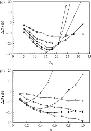
). Figure 1 shows the variations of the skin friction with the sensing plane location (
 $y_{s_{0}}^{+}$
) and proportional gain (
 $\unicode[STIX]{x1D6FC}$
), where
 $y_{s_{0}}^{+}=5{-}32$
and
 $\unicode[STIX]{x1D6FC}=0{-}1$
. When
 $\unicode[STIX]{x1D6FC}>1$
, all the cases considered diverged even if
 $y_{s_{0}}^{+}$
was small. The opposition control by Choi et al. (Reference Choi, Moin and Kim1994) corresponds to the case with
 $\unicode[STIX]{x1D6FC}=1$
, where the skin friction decreases at
 $y_{s_{0}}^{+}\lesssim 21$
but rapidly increases at
 $y_{s_{0}}^{+}>21$
(figure 1
a). The maximum skin-friction reduction of 29 % is obtained with the sensing plane at
 $y_{s_{0}}^{+}=15.4$
for
 $\unicode[STIX]{x1D6FC}=1$
. This sensing plane location is in good agreement with that of Hammond et al. (Reference Hammond, Bewley and Moin1998), and the amount of skin-friction reduction is slightly larger than that in Choi et al. (Reference Choi, Moin and Kim1994) and Hammond et al. (Reference Hammond, Bewley and Moin1998). This is because we perform simulations at
 $Re_{\unicode[STIX]{x1D70F}}=140$
, which is slightly lower than
 $Re_{\unicode[STIX]{x1D70F}}=180$
adopted in previous studies (Choi et al.
Reference Choi, Moin and Kim1994; Hammond et al.
Reference Hammond, Bewley and Moin1998; Chung & Talha Reference Chung and Talha2011), and the maximum amount of skin-friction reduction decreases with increasing Reynolds number (Chang et al.
Reference Chang, Collis and Ramakrishnan2002).
Variation of the skin friction with P control: (a) sensing location
 $y_{s_{0}}^{+}$
with ▫,
 $\unicode[STIX]{x1D6FC}=0.2$
;
 $\times$
, 0.4; ▿, 0.6;
 $+$
, 0.8; ○, 1.0; (b) proportional gain
 $\unicode[STIX]{x1D6FC}$
with ▫,
 $y_{s_{0}}^{+}=5.1$
;
 $\times$
, 9.3; ▿, 15.4;
 $+$
, 20.9; ○, 24.2; ♢, 32.

With increasing
 $y_{s_{0}}^{+}$
, the skin friction decreases and reaches its minimum at
 $y_{s_{0}}^{+}=y_{s,opt}^{+}$
. With further increase in
 $y_{s_{0}}^{+}$
, the skin friction starts to increase from its minimum and becomes larger than that without control. At larger
 $\unicode[STIX]{x1D6FC}\;({\leqslant}1)$
, the optimal sensing position resulting in minimum skin friction is lower (e.g.
 $y_{s,opt}^{+}\approx 15$
for
 $\unicode[STIX]{x1D6FC}=1$
and 20 for
 $\unicode[STIX]{x1D6FC}=0.4$
) (Chung & Talha Reference Chung and Talha2011) and the skin-friction reduction is larger. Thus, the optimal proportional gain providing maximum skin-friction reduction also depends on the sensing plane location. When
 $y_{s_{0}}^{+}\leqslant 15.4$
, the skin friction decreases more with larger
 $\unicode[STIX]{x1D6FC}$
, and the P control with
 $\unicode[STIX]{x1D6FC}=1$
shows the maximum skin-friction reduction. On the other hand, when
 $y_{s_{0}}^{+}>15.4$
, maximum skin-friction reduction is obtained with
 $\unicode[STIX]{x1D6FC}<1$
, although the amount of skin-friction reduction is smaller than that with
 $\unicode[STIX]{x1D6FC}=1$
at
 $y_{s_{0}}^{+}=15.4$
.
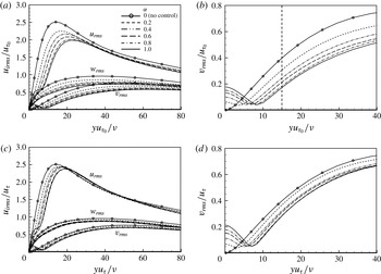
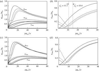
Figure 2 shows the root-mean-square (r.m.s.) velocity fluctuations normalized by
 $u_{\unicode[STIX]{x1D70F}_{0}}$
and
 $u_{\unicode[STIX]{x1D70F}}$
respectively for
 $y_{s_{0}}^{+}=15.4$
, at which the skin friction is minimum for
 $\unicode[STIX]{x1D6FC}=1$
. Here,
 $u_{\unicode[STIX]{x1D70F}}$
is the wall-shear velocity of controlled flow. The r.m.s. velocity fluctuations decrease more with larger
 $\unicode[STIX]{x1D6FC}$
(except very near the wall for the wall-normal velocity fluctuations due to the control input; figure 2
a,b). As observed in previous studies (Choi et al.
Reference Choi, Moin and Kim1994; Hammond et al.
Reference Hammond, Bewley and Moin1998; Chung & Talha Reference Chung and Talha2011), the P control establishes a ‘virtual wall’, showing a local minimum of
 $v_{rms}$
in between the physical wall and the sensing plane (figure 2
c,d). The location of the virtual wall moves away from the physical wall as
 $\unicode[STIX]{x1D6FC}$
increases. The outward shifts of the r.m.s. velocity fluctuations in the controlled cases also indicate the displaced virtual wall and thickened sublayer due to control (figure 2
c,d).
Root-mean-square velocity fluctuations with various values of
 $\unicode[STIX]{x1D6FC}$
at
 $y_{s_{0}}^{+}=15.4$
, normalized by (a,b)
 $u_{\unicode[STIX]{x1D70F}_{0}}$
and (c,d)
 $u_{\unicode[STIX]{x1D70F}}$
. The dashed vertical line in (b) denotes the location of the sensing plane.

It is interesting to mention the behaviour of the wall-normal velocity at the sensing plane (
 $v_{s,rms}$
) for different values of
 $\unicode[STIX]{x1D6FC}$
here. As described earlier, the sensing velocity
 $v_{s}$
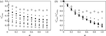
is considered as an error, and the purpose of control is to reduce this error. Figure 3 shows the r.m.s. sensing velocity fluctuations for different values of
 $\unicode[STIX]{x1D6FC}$
and
 $y_{s_{0}}^{+}$
. The sensing velocity fluctuations increase as
 $y_{s_{0}}^{+}$
increases and gradually decrease with increasing
 $\unicode[STIX]{x1D6FC}$
(figure 3
a). When
 $v_{s,rms}^{+}$
is normalized by the uncontrolled value at each
 $y_{s_{0}}^{+}$
, we obtain a simple relation as
 $$\begin{eqnarray}\frac{v_{s,rms}^{+}}{v_{s,rms_{0}}^{+}}\approx \frac{1}{(1+\unicode[STIX]{x1D6FC})},\end{eqnarray}$$
except for
 $y_{s_{0}}^{+}=18.0$
and 20.9 (figure 3
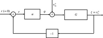
b). The relation in (3.1) may be explained by the block diagram provided in figure 4. From this figure, one can easily find that
 $v_{s}^{+}/v_{s_{o}}^{+}=G/(1+G\unicode[STIX]{x1D6FC})$
, where
 $G$
is the transfer function between
 $\unicode[STIX]{x1D701}=v_{s}^{+}$
and
 $\unicode[STIX]{x1D713}+v_{s_{o}}^{+}$
. In the absence of control (i.e.
 $\unicode[STIX]{x1D713}=0$
),
 $G=I$
. Thus, in cases where the sensing plane location is not far from the wall where the control is applied and the magnitude of the control input is not large,
 $G\approx 1$
, resulting in
 $v_{s}^{+}/v_{s_{o}}^{+}\approx 1/(1+\unicode[STIX]{x1D6FC})$
.
Root-mean-square sensing velocity fluctuations with various values of
 $\unicode[STIX]{x1D6FC}$
: (a)
 $v_{s,rms}$
normalized by
 $u_{\unicode[STIX]{x1D70F}}$
; (b)
 $v_{s,rms}^{+}$
normalized by the value without control (
 $v_{s,rms_{0}}^{+}$
); ▫,
 $y_{s_{0}}^{+}=5.1$
; ▴, 7.7;
 $\times$
, 9.3;
 $\ast$
, 11.1; ▽, 13.1; ●, 15.4;
 $+$
, 18.0; ♢, 20.9. In (b), the dashed line indicates
 $v_{s,rms}^{+}/v_{s,rms_{0}}^{+}=1/(1+\unicode[STIX]{x1D6FC})$
.

Block diagram of the P control.

3.2 Proportional–integral (PI) control
For PI control, the adjustable parameters are the proportional and integral gains (
 $\unicode[STIX]{x1D6FC},\unicode[STIX]{x1D6FD}$
), and the sensing plane location
 $y_{s_{0}}^{+}$
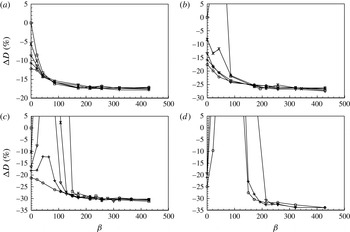
. Figure 5 shows the variation of the skin friction with these parameters, where the values of
 $\unicode[STIX]{x1D6FD}$
are normalized with
 $u_{\unicode[STIX]{x1D70F}_{0}}$
and
 $h$
. The cases with
 $\unicode[STIX]{x1D6FD}=0$
are the P control, and those with
 $\unicode[STIX]{x1D6FC}=0$
are the I control. When
 $\unicode[STIX]{x1D6FD}$
is sufficiently large (e.g.
 $\unicode[STIX]{x1D6FD}>200$
), the PI control provides more skin-friction reduction than the P control (
 $\unicode[STIX]{x1D6FD}=0$
) for all of the sensing locations considered, but the amount of skin-friction reduction is more or less saturated at large values of
 $\unicode[STIX]{x1D6FD}$
. On the other hand, the performance of the PI control is very sensitive to the sensing plane location,
 $y_{s_{0}}^{+}$
. At low values of
 $y_{s_{0}}^{+}$
(like at
 $y_{s_{0}}^{+}=5.1$
; figure 5
a), the skin friction decreases monotonically with increasing
 $\unicode[STIX]{x1D6FD}$
. However, as
 $y_{s_{0}}^{+}$
increases further (figure 5
b–d), the skin friction rapidly increases for a certain range of
 $\unicode[STIX]{x1D6FD}$
, and this range of
 $\unicode[STIX]{x1D6FD}$
becomes wider at higher sensing plane locations. It should also be noted that this increase in the skin friction is attenuated at larger values of
 $\unicode[STIX]{x1D6FC}$
. Among all the values of parameters considered, the maximum skin-friction reduction of approximately 34 % occurs at
 $(\unicode[STIX]{x1D6FC},\unicode[STIX]{x1D6FD},y_{s_{0}}^{+})=(1,428,11.1)$
. This amount of skin-friction reduction is larger than that with the optimal P control (29 %). On the other hand, PI controls at
 $y_{s_{0}}^{+}>12$
were unstable and diverged. We do not have a clear explanation for the variation of the skin friction with
 $\unicode[STIX]{x1D6FD}$
; i.e. the skin friction rapidly increases and the system becomes unstable at intermediate values of
 $\unicode[STIX]{x1D6FD}$
, and then the amount of skin-friction reduction is maximum at high values of
 $\unicode[STIX]{x1D6FD}$
. To further understand this behaviour, we apply PI controls to a linearized flow model having transient growth of disturbances. This result is given in § 4.
Variation of the skin friction with PI control: (a)
 $y_{s_{0}}^{+}=5.1$
; (b) 7.7; (c) 9.3; (d) 11.1; ▫,
 $\unicode[STIX]{x1D6FC}=0$
(I control);
 $\times$
, 0.2; ▿, 0.5;
 $+$
, 0.7; ○, 1.0. In (d), the cases of
 $\unicode[STIX]{x1D6FC}=0$
and 0.2 are not drawn because numerical solutions diverge for these cases.

Figure 6 shows the variation of the r.m.s. velocity fluctuations with a PI control, together with those from two P controls and no control. Here,
 $y_{s_{0}}^{+}=15.4$
is the optimal sensing plane location for the P control, and
 $y_{s_{0}}^{+}=11.1$
is that for the PI control. Due to the control (figure 6
a,b), the r.m.s. velocity fluctuations are overall reduced. Notably, unlike the P control, the r.m.s. wall-normal velocity fluctuations show a minimum at the sensing location with PI control, indicating that the I component of PI control indeed minimizes the steady-state error, i.e.
 $v_{s,rms}$
. The r.m.s. wall-normal velocity fluctuations at the wall, i.e.
 $v_{w_{rms}}$
, represent the magnitude of blowing and suction at the wall. For the P control, the magnitude of blowing and suction at the wall is identical to that of the sensing velocity fluctuations
 $v_{s,rms}$
. For the PI control,
 $v_{rms}$
at the wall is much larger than
 $v_{s,rms}$
because the control input should effectively reach the sensing location
 $y_{s_{0}}^{+}$
to minimize
 $v_{s,rms}$
. This is the reason why the PI control becomes unstable when the sensing location is farther away from the wall. The streamwise velocity fluctuations also increase very near the wall due to large
 $v_{rms}$
at the wall. As observed from P controls, the outward shifts of the r.m.s. velocity fluctuations in the PI control also indicate the displaced virtual wall and thickened sublayer due to control (figure 6
c,d).
Variation of the r.m.s. velocity fluctuations with PI control, normalized by (a,b)
 $u_{\unicode[STIX]{x1D70F}_{0}}$
and (c,d)
 $u_{\unicode[STIX]{x1D70F}}$
; ——, no control; – – – –, P control (
 $\unicode[STIX]{x1D6FC}=1$
,
 $y_{s_{0}}^{+}=11.1$
);
 $\cdots \cdots$
, P control (
 $\unicode[STIX]{x1D6FC}=1$
,
 $y_{s_{0}}^{+}=15.4$
); – - – - –, PI control (
 $\unicode[STIX]{x1D6FC}=1$
,
 $\unicode[STIX]{x1D6FD}=214$
,
 $y_{s_{0}}^{+}=11.1$
).

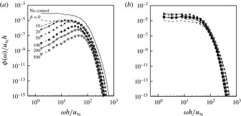
Figure 7 shows the energy spectra of the sensing and actuation velocity fluctuations of the PI control (
 $\unicode[STIX]{x1D6FC}=1$
and
 $\unicode[STIX]{x1D6FD}=0\sim 500$
;
 $y_{s_{0}}^{+}=9.3$
). With the PI control, the spectra of the sensing velocity fluctuations decrease with increasing
 $\unicode[STIX]{x1D6FD}$
, indicating that
 $v_{s,rms}$
also decreases with increasing
 $\unicode[STIX]{x1D6FD}$
. With the P control (
 $\unicode[STIX]{x1D6FD}=0$
), the energy at all of the frequency ranges is reduced from that of no control. With the addition of the I component, the energy is notably further reduced at low to intermediate frequencies. Moreover, this reduction of energy at low frequencies becomes more manifest at larger
 $\unicode[STIX]{x1D6FD}$
, and the frequency band for this reduction is bounded by
 $\unicode[STIX]{x1D714}h/u_{\unicode[STIX]{x1D70F}_{0}}\sim \unicode[STIX]{x1D6FD}$
, which suggests that the PI control reduces the strength of large-scale structures more effectively than the P control. It should also be noted that, unlike those of the sensing velocity, the energy spectra of the actuation velocity are not very different for different values of
 $\unicode[STIX]{x1D6FD}$
because of the integral component of PI control. In the P control with
 $\unicode[STIX]{x1D6FC}=1$
,
 $v_{w}$
is identical to
 $-v_{s}$
, and thus their energy spectra are the same. With the PI control, however,
 $v_{w}$
is mainly determined by the integral component of
 $v_{s}$
, e.g. the r.m.s. value of the integral component is five times that of the proportional component for
 $\unicode[STIX]{x1D6FC}=1$
and
 $\unicode[STIX]{x1D6FD}=200$
at
 $y_{s_{0}}^{+}=9.3$
.
Energy spectra of the sensing and actuation velocities from PI control (
 $y_{s_{0}}^{+}=9.3,\unicode[STIX]{x1D6FC}=1$
): (a) sensing velocity (
 $v_{s}$
); (b) actuation velocity (
 $v_{w}$
).

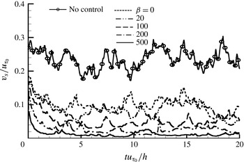
Figure 8 shows the time histories of the sensing velocities for the P (
 $\unicode[STIX]{x1D6FD}=0$
) and PI (
 $\unicode[STIX]{x1D6FD}\neq 0$
) controls, together with that for no control. In control theory (Franklin, Powell & Emami-Naeini Reference Franklin, Powell and Emami-Naeini1994), the settling time is defined as the time required for the transient to decay to within a few per cent (usually 5 % or 2 %) of the final value. However, since the fluctuation magnitude itself is often larger than that amount in turbulent flow, the settling time may not be a proper choice as the response time of the control. Instead, the rise time, which is the time required for the system to reach the vicinity of its new set point, may be more appropriate. It is clear from figure 8 that larger
 $\unicode[STIX]{x1D6FD}$
has shorter rise time, indicating that larger
 $\unicode[STIX]{x1D6FD}$
can control flow structures having smaller integral time (or streamwise length) scales. This is consistent with the variation of the energy spectra of
 $v_{s}$
with
 $\unicode[STIX]{x1D6FD}$
in figure 7, i.e. the reduction of energy at low to intermediate frequencies by PI control is bounded by
 $\unicode[STIX]{x1D714}h/u_{\unicode[STIX]{x1D70F}_{0}}\sim \unicode[STIX]{x1D6FD}$
. This rise time appears to be shorter than
 $tu_{\unicode[STIX]{x1D70F}_{0}}/h=5$
(
 $t^{+}=700$
) for all of the cases considered. For example, in the case of
 $\unicode[STIX]{x1D6FD}=500$
, the rise time may be
 $tu_{\unicode[STIX]{x1D70F}_{0}}/h=0.5\sim 1$
(
 $t^{+}=70{-}140$
). Considering that the eddy turnover time in the near-wall region is
 $t^{+}\approx 80$
, the control response time to reach an equilibrium state is comparable to or longer than the near-wall eddy turnover time. For the linearized flow model discussed in § 4, the frequency responses of the P and PI controls are given (see below).
Time histories of the sensing velocities (
 $y_{s_{0}}^{+}=9.3$
,
 $\unicode[STIX]{x1D6FC}=1$
).

Instantaneous vortical structures identified by isosurfaces of
 $\unicode[STIX]{x1D706}_{2}$
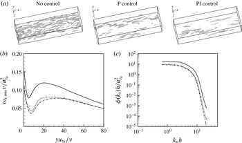
(Jeong & Hussain Reference Jeong and Hussain1995) and the r.m.s. profiles and power spectra of the streamwise vorticity fluctuations for the cases of no, P and PI controls are shown in figure 9. The P and PI controls shown in this figure produced nearly the same amounts of drag reduction (approximately 29 %). As shown, near-wall vortical structures and the strength of the streamwise vorticity are significantly weakened by the P and PI controls. It is also notable that the reductions of power of the streamwise vorticity from the P and PI controls are very similar to each other, although the changes in the sensing velocities are quite different (see, for example, figure 7
a). This indicates that the near-wall vortical structures are weakened and deformed according to the controls, but not very differently depending on the P and PI controls (if the amount of drag reduction is same), even if their target (i.e. sensing) velocities are changed quite differently.
Instantaneous vortical structures and streamwise vorticity: (a) vortical structures (isosurfaces of
 $\unicode[STIX]{x1D706}_{2}=-0.2$
); (b) r.m.s. streamwise vorticity fluctuations; (c) power spectra of the streamwise vorticity fluctuations. In (b,c): ——, no control; – – – –, P control (
 $\unicode[STIX]{x1D6FC}=1$
,
 $y_{s_{0}}^{+}=15.4$
); – - – - –, PI control (
 $\unicode[STIX]{x1D6FC}=1$
,
 $\unicode[STIX]{x1D6FD}=214$
,
 $y_{s_{0}}^{+}=9.3$
). In (c), the spectra for the cases of no, P and PI controls are from the locations where the r.m.s. streamwise vorticity fluctuations are local maxima, i.e.
 $yu_{\unicode[STIX]{x1D70F}_{0}}/\unicode[STIX]{x1D708}=19.1$
, 25.6 and 33.7 respectively.

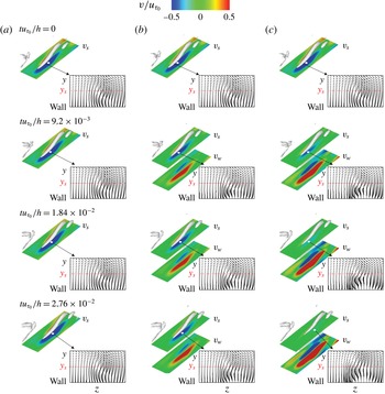
Figure 10 shows the evolution of a near-wall vortex and contours of
 $v_{s}$
and
 $v_{w}$
, together with cross-flow vectors (
 $v,w$
) on a
 $(y,z)$
plane. These time sequences of flow fields are obtained right after the P and PI controls are applied. As shown, in the case of no control, the near-wall vortex generates sweep and ejection motions on its right and left sides respectively and travels downstream. In the case of P control (
 $y_{s_{0}}^{+}=9.3$
and
 $\unicode[STIX]{x1D6FC}=1$
; figure 10
b), the actuation velocity is
 $180^{\circ }$
out of phase with the sensing velocity, and prevents the sweep and ejection motions induced by the streamwise vortex, which lifts up the centre of the streamwise vortex away from the wall. In the meantime, the magnitude of the actuation velocity at the wall decreases as the streamwise vortex becomes weaker and is located further away from the wall. In the case of PI control (
 $y_{s_{0}}^{+}=9.3$
,
 $\unicode[STIX]{x1D6FC}=1$
and
 $\unicode[STIX]{x1D6FD}=214$
; figure 10
c), the actuation velocity is similar to that of P control right after the control, but becomes stronger in time due to the time integration of sweep and ejection motions by the streamwise vortex. This actuation lifts up the vortex further away from the wall than the P control does, and the strength of the vortex is also much weaker than that by P control. It should be noted that, after a short time (
 $tu_{\unicode[STIX]{x1D70F}_{0}}/h=0.0276$
), the PI control successfully removes the wall-normal velocity fluctuations on the sensing plane.
Evolution of a near-wall vortex and contours of the wall-normal velocities on the sensing plane (
 $y^{+}=y_{s_{0}}^{+}$
) and the wall, together with cross-flow vectors (
 $v,w$
) on a
 $(y,z)$
plane at a streamwise location where maximum
 $|v_{s}|$
is observed (denoted as a white dot in each figure): (a) no control; (b) P control (
 $y_{s_{0}}^{+}=9.3,\unicode[STIX]{x1D6FC}=1$
); (c) PI control (
 $y_{s_{0}}^{+}=9.3,\unicode[STIX]{x1D6FC}=1,\unicode[STIX]{x1D6FD}=214$
). The contours of the wall-normal velocities and the cross-flow vectors are drawn in the domain sizes of
 $(\unicode[STIX]{x1D6FF}_{x}/h,\unicode[STIX]{x1D6FF}_{z}/h)=(1.62,0.491)$
and
 $(\unicode[STIX]{x1D6FF}_{z}/h,\unicode[STIX]{x1D6FF}_{y}/h)=(0.491,0.135)$
respectively.

The sweep motion induced by the near-wall vortical structure requires a time to reach at the wall and generate high skin friction there. Therefore, Lee (Reference Lee2015) suggested a P control with a sensor located upstream of the actuator, i.e.
 $v_{w}(x,z,t)=-v_{s}(x-x_{s},z,t)$
, where
 $x_{s}~({>}0)$
is the streamwise distance between the sensor and the actuator. This control produced a slightly larger drag reduction. On the other hand, in the present PI control, the sensing velocity is integrated over time at a given sensing location. Then, one may wonder whether the present PI control does not work properly because the near-wall vortical structures are inclined in the wall-normal direction. However, it is well known that the inclination angle of near-wall structures is only
 $9^{\circ }$
(Jeong et al.
Reference Jeong, Hussain, Schoppa and Kim1997) and the statistical location of their centre is approximately 20 in wall units (Kim, Moin & Moser Reference Kim, Moin and Moser1987). Since the sensing plane considered in this study is much lower than this location, the control results are not greatly affected by the inclination of the structures. However, when the sensing location moves away from the wall, the integrated actuation velocity becomes too large even in the absence of near-wall vortices, which makes the system unstable.
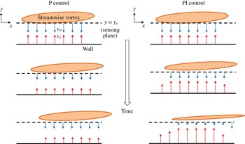
Figure 11 shows the mechanisms responsible for the skin-friction reduction by P and PI controls. In this figure, we draw the streamwise evolution of a tilted elongated near-wall streamwise vortex due to P and PI controls. Since a downwash motion towards the wall is induced by this streamwise vortex, the P or PI control provides a blowing underneath this downwash motion and attenuates this motion in time. With the P control (
 $\unicode[STIX]{x1D6FC}=1$
), at each instant, the actuation
 $v_{w}$
is opposite to the sensing velocity
 $v_{s}$
. When
 $v_{s}$
decreases due to the P control,
 $v_{w}$
also decreases in time. Therefore, the P control cannot eliminate
 $v_{s}$
, but drives the wall-normal velocity at
 $y\approx y_{s}/2$
to nearly zero. On the other hand, with the PI control,
 $v_{w}$
keeps increasing until
 $v_{s}$
becomes zero, because the I component of the PI control accumulates past values of
 $y_{s}$
. Thus, successful PI controls remove the wall-normal motion at the sensing plane and reduce the strength of near-wall streamwise vortices, resulting in more reduction in the skin friction than the P control.
Schematic diagram of the mechanisms responsible for the skin-friction reduction by P and PI controls. The streamwise vortex shown in this figure has positive streamwise vorticity and its centre is located behind the
 $(x,y)$
plane.

4 Proportional–integral control based on a linearized flow model
In the previous section, we showed that the PI control performs better than the P control in reducing the skin friction in a turbulent channel flow. Although turbulent channel flow is overall highly nonlinear, the underlying mechanism of drag reduction by the present control may be linear. Therefore, to further understand the effects of the P and PI controls, we consider a flow model linearized from the Navier–Stokes equations,
 $$\begin{eqnarray}\frac{\unicode[STIX]{x2202}\boldsymbol{u}}{\unicode[STIX]{x2202}t}+U(y)\frac{\unicode[STIX]{x2202}\boldsymbol{u}}{\unicode[STIX]{x2202}x}+\left(v\frac{\text{d}U}{\text{d}y},0,0\right)=-\unicode[STIX]{x1D735}p+\frac{1}{Re_{\unicode[STIX]{x1D70F}}}\unicode[STIX]{x0394}\boldsymbol{u},\end{eqnarray}$$
where
 $U(y)$
is the mean velocity profile of turbulent channel flow,
 $\boldsymbol{u}=(u,v,w)$
is the velocity vector of the perturbations,
 $p$
is the pressure perturbation and
 $\unicode[STIX]{x0394}=\unicode[STIX]{x1D6FB}^{2}=\unicode[STIX]{x2202}^{2}/\unicode[STIX]{x2202}x^{2}+\unicode[STIX]{x2202}^{2}/\unicode[STIX]{x2202}y^{2}+\unicode[STIX]{x2202}^{2}/\unicode[STIX]{x2202}z^{2}$
.
For turbulent channel flow that is statistically homogeneous in the streamwise and spanwise directions, the Navier–Stokes equations are reformulated with the Fourier modes of the wall-normal velocity
 $\hat{v}$
and wall-normal vorticity
 $\hat{\unicode[STIX]{x1D714}}_{y}$
. Then, the linearized Navier–Stokes equations (4.1) are written in the following operator form (Schmid & Henningson Reference Schmid and Henningson2001):
 $$\begin{eqnarray}\frac{\unicode[STIX]{x2202}}{\unicode[STIX]{x2202}t}\left[\begin{array}{@{}c@{}}\hat{v}\\ \hat{\unicode[STIX]{x1D714}}_{y}\end{array}\right]=\left[\begin{array}{@{}cc@{}}L_{os} & 0\\ L_{c} & L_{sq}\end{array}\right]\left[\begin{array}{@{}c@{}}\hat{v}\\ \hat{\unicode[STIX]{x1D714}}_{y}\end{array}\right],\end{eqnarray}$$
where
 $L_{os}$
,
 $L_{sq}$
and
 $L_{c}$
are the Orr–Sommerfeld, Squire and linear coupling operators respectively, and they are given by
 $$\begin{eqnarray}\displaystyle & \displaystyle L_{os}=\hat{\unicode[STIX]{x0394}}^{-1}\left(-\text{i}k_{x}U\hat{\unicode[STIX]{x0394}}+\text{i}k_{x}U^{\prime \prime }+\frac{1}{Re_{\unicode[STIX]{x1D70F}}}\hat{\unicode[STIX]{x0394}}^{2}\right), & \displaystyle\end{eqnarray}$$
 $$\begin{eqnarray}\displaystyle & \displaystyle L_{sq}=-\text{i}k_{x}U+\frac{1}{Re_{\unicode[STIX]{x1D70F}}}\hat{\unicode[STIX]{x0394}}, & \displaystyle\end{eqnarray}$$
 $$\begin{eqnarray}\displaystyle & \displaystyle L_{c}=\text{i}k_{z}U^{\prime }. & \displaystyle\end{eqnarray}$$
Here, the superscript (
 $^{\prime }$
) denotes
 $\text{d}/\text{d}y$
,
 $k_{x}$
and
 $k_{z}$
are the streamwise and spanwise wavenumbers respectively, and
 $\hat{\unicode[STIX]{x0394}}=\unicode[STIX]{x2202}^{2}/\unicode[STIX]{x2202}y^{2}-k_{x}^{2}-k_{z}^{2}$
.
The linearized Navier–Stokes equations with a control input
 $\boldsymbol{q}$
can be written in the following state-space representation (Bewley & Liu Reference Bewley and Liu1998; Lim & Kim Reference Lim and Kim2004):
 $$\begin{eqnarray}\displaystyle & \dot{\boldsymbol{x}}=\unicode[STIX]{x1D63C}\boldsymbol{x}+\unicode[STIX]{x1D63D}\boldsymbol{q}, & \displaystyle\end{eqnarray}$$
 $$\begin{eqnarray}\displaystyle & \boldsymbol{y}=\unicode[STIX]{x1D63E}\boldsymbol{x}, & \displaystyle\end{eqnarray}$$
where
 $\boldsymbol{x}=(\hat{v},\hat{\unicode[STIX]{x1D714}}_{y})^{\text{T}}$
is the state of the system,
 $\boldsymbol{q}$
is the control input
 $\hat{v}_{w}$
(blowing and suction at the wall) and
 $\boldsymbol{y}$
is the control output
 $\hat{v}_{s}$
(sensing velocity). The operators
 $\unicode[STIX]{x1D63C}$
and
 $\unicode[STIX]{x1D63D}$
are the matrices for internal and boundary grid points respectively, which are obtained by applying spatial discretizations to (4.2). The details of the matrices
 $\unicode[STIX]{x1D63C}$
and
 $\unicode[STIX]{x1D63D}$
can be found in Bewley & Liu (Reference Bewley and Liu1998). The observation operator
 $\unicode[STIX]{x1D63E}$
is constructed once the sensing location
 $y_{s}$
is chosen; the components of
 $\unicode[STIX]{x1D63E}$
are 1 only at the sensing location and 0 otherwise. For P control, the control input is
 $\boldsymbol{q}=-\unicode[STIX]{x1D6FC}\boldsymbol{y}=-\unicode[STIX]{x1D6FC}\unicode[STIX]{x1D63E}\boldsymbol{x}$
. By substituting this into (4.6), the system equation becomes
 $$\begin{eqnarray}\dot{\boldsymbol{x}}=(\unicode[STIX]{x1D63C}-\unicode[STIX]{x1D6FC}\unicode[STIX]{x1D63D}\unicode[STIX]{x1D63E})\boldsymbol{x}.\end{eqnarray}$$
For PI control, we introduce a vector
 $\boldsymbol{z}$
satisfying
 $\dot{\boldsymbol{z}}=\boldsymbol{y}=\unicode[STIX]{x1D63E}\boldsymbol{x}$
. Then, the control input becomes
 $\boldsymbol{q}=-\unicode[STIX]{x1D6FC}\boldsymbol{y}-\unicode[STIX]{x1D6FD}\boldsymbol{z}$
. By substituting this into (4.6), the system equation is given as
 $$\begin{eqnarray}\left[\begin{array}{@{}c@{}}\dot{\boldsymbol{x}}\\ \dot{\boldsymbol{z}}\end{array}\right]=\left[\begin{array}{@{}cc@{}}\unicode[STIX]{x1D63C}-\unicode[STIX]{x1D6FC}\unicode[STIX]{x1D63D}\unicode[STIX]{x1D63E} & -\unicode[STIX]{x1D6FD}\unicode[STIX]{x1D63D}\\ \unicode[STIX]{x1D63E} & \boldsymbol{ 0}\end{array}\right]\left[\begin{array}{@{}c@{}}\boldsymbol{x}\\ \boldsymbol{ z}\end{array}\right].\end{eqnarray}$$
Thus, the modified system matrix for P control is
 $\unicode[STIX]{x1D63C}_{c}=\unicode[STIX]{x1D63C}-\unicode[STIX]{x1D6FC}\unicode[STIX]{x1D63D}\unicode[STIX]{x1D63E}$
and that for PI control is
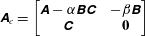 $\unicode[STIX]{x1D63C}_{c}=\left[\begin{array}{@{}cc@{}}\unicode[STIX]{x1D63C}-\unicode[STIX]{x1D6FC}\unicode[STIX]{x1D63D}\unicode[STIX]{x1D63E} & -\unicode[STIX]{x1D6FD}\unicode[STIX]{x1D63D}\\ \unicode[STIX]{x1D63E} & \boldsymbol{ 0}\end{array}\right]$
.
The model based on the linearized equation may miss some nonlinear characteristics existing in turbulent flow, but it is well known that the linear process plays an important role in generating and sustaining near-wall turbulent structures (Reddy & Henningson Reference Reddy and Henningson1993; Kim & Lim Reference Kim and Lim2000). Many studies (Hu & Bau Reference Hu and Bau1994; Joshi et al. Reference Joshi, Speyer and Kim1997; Bewley & Liu Reference Bewley and Liu1998; Lee et al. Reference Lee, Cortelezzi, Kim and Speyer2001; Högberg et al. Reference Högberg, Bewley and Henningson2003; Kim & Bewley Reference Kim and Bewley2007) have investigated various control methods aiming at altering this linear process based on a flow model from linearized equations, and have shown that some of the controls are successful in changing turbulent channel and boundary layer flows. In this section, we apply the P and PI controls to the flow models, (4.8) and (4.9), obtained from the linearized equations, and compare the results with those from direct solutions of the Navier–Stokes equations discussed in § 3.
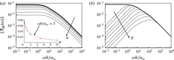
The
 $L_{2}$
-norm of the frequency response of the system output to sinusoidal noise: (a) P control (
 $\unicode[STIX]{x1D6FC}=0.1$
, 0.2, 0.5, 1, 2, 5, and 10); (b) I control (
 $\unicode[STIX]{x1D6FD}=1$
, 2, 5, 10, 20, 50, 100, 200, and 500). The wavenumber pair of the system is
 $(k_{x},k_{z})=(0,8.5)$
and
 $y_{s_{0}}^{+}=10.7$
. The thick solid line corresponds to the case of no control. In (a), the inset shows the variation of
 $\Vert \unicode[STIX]{x1D64F}_{\hat{\boldsymbol{y}}\hat{\boldsymbol{n}}}\Vert$
with
 $\unicode[STIX]{x1D6FC}$
at
 $\unicode[STIX]{x1D714}h/u_{\unicode[STIX]{x1D70F}_{0}}=1$
, together with a dotted line of
 $\Vert \unicode[STIX]{x1D64F}_{\hat{\boldsymbol{y}}\hat{\boldsymbol{n}}}\Vert =1/(1+\unicode[STIX]{x1D6FC})$
.

4.1 Frequency response
The frequency response of the system is obtained from the linearized flow model, (4.6) and (4.7). With a harmonic control input
 $\hat{\boldsymbol{q}}(\unicode[STIX]{x1D714})$
, the control output after enough time is
 $\hat{\boldsymbol{y}}=\unicode[STIX]{x1D64F}_{\hat{\boldsymbol{y}}\hat{\boldsymbol{q}}}\hat{\boldsymbol{q}}$
, where the transfer function is given as
 $\unicode[STIX]{x1D64F}_{\hat{\boldsymbol{y}}\hat{\boldsymbol{q}}}=\unicode[STIX]{x1D63E}(\text{i}\unicode[STIX]{x1D714}\unicode[STIX]{x1D644}-\unicode[STIX]{x1D63C})^{-1}\unicode[STIX]{x1D63D}$
. In this case, the frequency response,
 $\Vert \hat{\boldsymbol{y}}\Vert /\Vert \hat{\boldsymbol{q}}\Vert$
, is defined by the
 $L_{2}$
-norm of the transfer function,
 $\Vert \unicode[STIX]{x1D64F}_{\hat{\boldsymbol{y}}\hat{\boldsymbol{q}}}(\unicode[STIX]{x1D714})\Vert =\sqrt{\text{trace}(\unicode[STIX]{x1D64F}_{\hat{\boldsymbol{y}}\hat{\boldsymbol{q}}}^{\ast }(\unicode[STIX]{x1D714})\unicode[STIX]{x1D64F}_{\hat{\boldsymbol{y}}\hat{\boldsymbol{q}}}(\unicode[STIX]{x1D714}))}$
, where
 $^{\ast }$
denotes the complex conjugate. Similarly, when we consider noise in the system, the state-space equation (4.6) becomes
 $$\begin{eqnarray}\dot{\boldsymbol{x}}=\unicode[STIX]{x1D63C}\boldsymbol{x}+\unicode[STIX]{x1D63D}\boldsymbol{q}+\unicode[STIX]{x1D642}\boldsymbol{n}.\end{eqnarray}$$
Here,
 $\boldsymbol{n}$
is the noise in the system and
 $\unicode[STIX]{x1D642}$
is the square root of the expected covariance of the noise. In the present study,
 $\unicode[STIX]{x1D642}$
is assumed to have simple covariance such as
 $\unicode[STIX]{x1D642}=\unicode[STIX]{x1D644}$
. Without control input (
 $\hat{\boldsymbol{q}}=0$
), the transfer function of the system output coming from a sinusoidal noise
 $\boldsymbol{n}(\unicode[STIX]{x1D714})$
can be obtained from
 $\unicode[STIX]{x1D64F}_{\hat{\boldsymbol{y}}\hat{\boldsymbol{n}}}(\unicode[STIX]{x1D714})=\unicode[STIX]{x1D63E}(\text{i}\unicode[STIX]{x1D714}\unicode[STIX]{x1D644}-\unicode[STIX]{x1D63C})^{-1}\unicode[STIX]{x1D642}$
. For the control, we use the modified transfer function
 $\unicode[STIX]{x1D63C}_{c}$
instead of
 $\unicode[STIX]{x1D63C}$
. For the PI control, we also use
 $\unicode[STIX]{x1D63E}^{\prime }=[\unicode[STIX]{x1D63E}\;\;\mathbf{0}]$
and
 $\unicode[STIX]{x1D642}^{\prime }=\left[\begin{array}{@{}c@{}}\unicode[STIX]{x1D642}\\ \mathbf{0}\end{array}\right]$
instead of
 $\unicode[STIX]{x1D63E}$
and
 $\unicode[STIX]{x1D642}$
respectively to match the matrix size. The
 $L_{2}$
-norm of the transfer function from noise is determined by
 $\Vert \unicode[STIX]{x1D64F}_{\hat{\boldsymbol{y}}\hat{\boldsymbol{n}}}(\unicode[STIX]{x1D714})\Vert =\sqrt{\text{trace}(\unicode[STIX]{x1D64F}_{\hat{\boldsymbol{y}}\hat{\boldsymbol{n}}}^{\ast }(\unicode[STIX]{x1D714})\unicode[STIX]{x1D64F}_{\hat{\boldsymbol{y}}\hat{\boldsymbol{n}}}(\unicode[STIX]{x1D714}))}$
. The value of
 $(1/2\unicode[STIX]{x03C0})\int _{-\infty }^{\infty }\Vert \unicode[STIX]{x1D64F}_{\hat{\boldsymbol{y}}\hat{\boldsymbol{n}}}(\unicode[STIX]{x1D714})\Vert ^{2}\,\text{d}\unicode[STIX]{x1D714}$
is referred to as the square of the
 ${\mathcal{H}}_{2}$
-norm of the transfer function (Doyle et al.
Reference Doyle, Glover, Khargonekar and Francis1989; Bewley & Liu Reference Bewley and Liu1998).
Figure 12 shows the variation of
 $\Vert \unicode[STIX]{x1D64F}_{\hat{\boldsymbol{y}}\hat{\boldsymbol{n}}}(\unicode[STIX]{x1D714})\Vert$
with the proportional gain
 $\unicode[STIX]{x1D6FC}$
and the integral gain
 $\unicode[STIX]{x1D6FD}$
for a wavenumber pair of
 $(k_{x},k_{z})=(0,8.5)$
and
 $y_{s_{0}}^{+}=10.7$
. This wavenumber pair corresponds to that of maximum transient energy growth (see below). As shown, the P and I controls reduce
 $\Vert \unicode[STIX]{x1D64F}_{\hat{\boldsymbol{y}}\hat{\boldsymbol{n}}}(\unicode[STIX]{x1D714})\Vert$
at almost all frequencies except very high frequencies for the I control. For the P control, the magnitude of the frequency response decreases as
 $1/(1+\unicode[STIX]{x1D6FC})$
for all frequencies (see, for example, the inset in figure 12
a). It should be noted that this linear system shows continuous reduction of the magnitude even at very large
 $\unicode[STIX]{x1D6FC}$
, although P control with
 $\unicode[STIX]{x1D6FC}>1$
makes the system unstable for turbulent channel flow. For the I control, the magnitude of frequency response decreases at
 $\unicode[STIX]{x1D714}h/u_{\unicode[STIX]{x1D70F}_{0}}\leqslant \unicode[STIX]{x1D6FD}$
. These results are very similar to the modifications of the energy spectra of the sensing velocity fluctuations in turbulent channel flow by P and PI controls (figure 7).
4.2 Transient growth of disturbances
It is generally accepted that the transient growth of optimal disturbances in a linearized flow model shows the formation of streaky structures (Butler & Farrell Reference Butler and Farrell1992; Kim, Choi & Kim Reference Kim, Choi and Kim2016), which play a key role in the regeneration of near-wall turbulent structures. This transient growth of a disturbance has been shown to be suppressed by opposition control (Farrell & Ioannou Reference Farrell and Ioannou1996; Lim & Kim Reference Lim and Kim2004) and by a linear optimal control (LQG) (Bewley & Liu Reference Bewley and Liu1998; Lim & Kim Reference Lim and Kim2004). In this subsection, we discuss the effects of P and PI controls on the transient growth of disturbances. We calculate the transient-growth ratio of a disturbance
 $G$
, defined as the ratio of its kinetic energy at a given time to its initial value, by means of singular value decomposition (SVD) (Lim & Kim Reference Lim and Kim2004):
 $$\begin{eqnarray}G(k_{x},k_{z},t)=\sup _{E(k_{x},k_{z},0)\neq 0}\frac{E(k_{x},k_{z},t)}{E(k_{x},k_{z},0)},\end{eqnarray}$$
where the kinetic energy density of a disturbance is
 $$\begin{eqnarray}E=\int _{-1}^{1}\left[\hat{v}^{\ast }\hat{v}+\frac{1}{k_{x}^{2}+k_{z}^{2}}\left(\frac{\unicode[STIX]{x2202}\hat{v}^{\ast }}{\unicode[STIX]{x2202}y}\frac{\unicode[STIX]{x2202}\hat{v}}{\unicode[STIX]{x2202}y}+\hat{\unicode[STIX]{x1D714}}_{y}^{\ast }\hat{\unicode[STIX]{x1D714}}_{y}\right)\right]\text{d}y.\end{eqnarray}$$
The detailed procedures for obtaining
 $G$
are shown in appendix A. The performance of P and PI controls is evaluated by comparing the largest energy growth ratios for various control parameters such as the sensing plane location
 $y_{s_{0}}^{+}$
, and the control gains
 $\unicode[STIX]{x1D6FC}$
and
 $\unicode[STIX]{x1D6FD}$
.
Butler & Farrell (Reference Butler and Farrell1993) constrained the growth time of disturbances at
 $t^{+}=80$
, which corresponds to the eddy turnover time in the near-wall region in turbulent channel or boundary layer flow, and obtained an optimal spanwise wavelength of
 $\unicode[STIX]{x1D706}_{z}^{+}\approx 110$
, which is approximately the typical spanwise spacing of the near-wall streaks. Therefore, we compare the maximum energy growth ratio,
 $\text{Max}(G(t))(=\sup _{k_{x},k_{z}}G(k_{x},k_{z},t))$
, at
 $t^{+}=80$
for different control parameters, to evaluate their performance. The variation of
 $\text{Max}(G(t^{+}=80))$
with
 $y_{s_{0}}^{+}$
for the P and PI controls is shown in figure 13. The variation of the maximum growth ratio is defined as
 $$\begin{eqnarray}\unicode[STIX]{x0394}\text{Max}(G)(\%)=\frac{\text{Max}(G)-\text{Max}(G)_{no}}{\text{Max}(G)_{no}}\times 100,\end{eqnarray}$$
where
 $\text{Max}(G(t^{+}=80))_{no}=36.3$
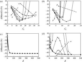
. For the P control (figure 13
a), the variation of
 $\text{Max}(G)$
is very similar to that of the skin friction in turbulent channel flow (figure 1
a). That is,
 $\text{Max}(G)$
decreases with increasing
 $y_{s_{0}}^{+}$
until it reaches a minimum, and then it rapidly increases with further increase in
 $y_{s_{0}}^{+}$
. The largest suppression of
 $\text{Max}(G)$
is 42.5 % at
 $y_{s_{0}}^{+}=13.4$
. The PI control shows a slightly better performance in suppressing
 $\text{Max}(G)$
than the P control when
 $y_{s_{0}}^{+}\leqslant 8.2$
(figure 13
b). In this range of
 $y_{s_{0}}^{+}$
,
 $\text{Max}(G)$
decreases with increasing
 $\unicode[STIX]{x1D6FD}$
. The maximum suppression of
 $\text{Max}(G)$
is 45.4 % at
 $y_{s_{0}}^{+}=8.2$
with
 $\unicode[STIX]{x1D6FD}=500$
. However, when
 $y_{s_{0}}^{+}>8.2$
, the PI control increases
 $\text{Max}(G(t))$
drastically. All of these behaviours from P and PI controls are very similar to those observed in turbulent channel flow. When
 $y_{s_{0}}^{+}=6.0$
(figure 13
c), the PI controls (i.e. non-zero
 $\unicode[STIX]{x1D6FD}$
) show better performance than the P control (
 $\unicode[STIX]{x1D6FD}=0$
), but this enhanced performance is nearly insensitive to the values of
 $\unicode[STIX]{x1D6FC}$
and
 $\unicode[STIX]{x1D6FD}$
considered. When
 $y_{s_{0}}^{+}=8.2$
(figure 13
d), the PI control increases
 $\text{Max}(G(t))$
for a range of
 $\unicode[STIX]{x1D6FD}$
, and this range becomes wider as
 $\unicode[STIX]{x1D6FC}$
decreases. At a sufficiently large
 $\unicode[STIX]{x1D6FD}~({\geqslant}300)$
, the PI control suppresses
 $\text{Max}(G(t))$
for all values of
 $\unicode[STIX]{x1D6FC}$
considered. This behaviour is also very similar to that in turbulent channel flow (figure 5).
Variation of
 $\text{Max}(G(t^{+}=80))$
with
 $y_{s_{0}}^{+}$
(a,b) and
 $\unicode[STIX]{x1D6FD}$
(c,d): (a) P control (▫,
 $\unicode[STIX]{x1D6FC}=0.2$
;
 $\times$
, 0.4; ▿, 0.6;
 $+$
, 0.8; ○, 1.0); (b) PI control with
 $\unicode[STIX]{x1D6FC}=1$
(▫,
 $\unicode[STIX]{x1D6FD}=0$
;
 $\times$
, 10; ▿, 20;
 $+$
, 50; ○, 100;
 $\triangle$
, 200; ♢, 500); (c) PI control for
 $y_{s_{0}}^{+}=6.0$
; (d) PI control for
 $y_{s_{0}}^{+}=8.2$
. In (c,d), ▫,
 $\unicode[STIX]{x1D6FC}=0$
;
 $\times$
, 0.2; ▿, 0.5;
 $+$
, 0.7; ○, 1.0.

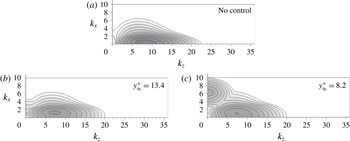
Figure 14 shows the contours of the energy growth ratio
 $G(t^{+}=80)$
on the wavenumber (
 $k_{x},k_{z}$
) plane. For no control, the disturbance with
 $(k_{x},k_{z})=(0,8.5)$
results in a maximum transient energy growth ratio of
 $\text{Max}(G)_{no}=36.3$
. Its corresponding spanwise wavelength,
 $\unicode[STIX]{x1D706}_{z}^{+}=104$
, is approximately equal to that of the wall-layer streaks. The P and PI controls with proper sensing locations suppress the growth of this disturbance. Accordingly,
 $\text{Max}(G(t))$
occurs at different wavenumber pairs for the P and PI controls. For the P control (
 $\unicode[STIX]{x1D6FC}=1$
,
 $y_{s_{0}}^{+}=13.4$
; figure 14
b),
 $\text{Max}(G)=20.8$
at
 $(k_{x},k_{z})=(1.4,7.25)$
, and for the PI control (
 $\unicode[STIX]{x1D6FC}=1$
,
 $\unicode[STIX]{x1D6FD}=200$
,
 $y_{s_{0}}^{+}=8.2$
; figure 14
c),
 $\text{Max}(G)=20.0$
at
 $(k_{x},k_{z})=(1.0,7.5)$
. This indicates that the P and PI controls decrease the spanwise wavenumber (or increase the spanwise wavelength) corresponding to maximum growth, which is similar to the increase in the streak spacing in turbulent channel flow by these controls.
Contours of
 $G(t^{+}=80)$
on the (
 $k_{x},k_{z}$
) plane: (a) no control; (b) P control with
 $\unicode[STIX]{x1D6FC}=1$
; (c) PI control with
 $\unicode[STIX]{x1D6FC}=1$
and
 $\unicode[STIX]{x1D6FD}=200$
. The contour levels are logarithmically distributed from
 $10^{0.4}$
to
 $10^{1.5}$
with exponent increments of 0.1.

5 Conclusions
In the present study, we applied a linear PI control to a turbulent channel flow at
 $Re_{\unicode[STIX]{x1D70F}}=140$
to reduce the skin friction on the wall. Similarly to the opposition control introduced by Choi et al. (Reference Choi, Moin and Kim1994), the wall-normal velocity on a sensing plane above the wall was detected for sensing, and blowing and suction (i.e. control input) at the wall was determined by the P or PI control. We investigated the effects of the proportional gain
 $\unicode[STIX]{x1D6FC}$
, the integral gain
 $\unicode[STIX]{x1D6FD}$
and the sensing plane location
 $y_{s_{0}}^{+}$
on the flow and skin friction. The P controls successfully reduced the strength of near-wall streamwise vortices and the skin friction when a proper sensing location and proportional feedback gain were chosen (Choi et al.
Reference Choi, Moin and Kim1994; Chung & Talha Reference Chung and Talha2011; Deng et al.
Reference Deng, Xu, Huang and Cui2014). The r.m.s. sensing velocity fluctuations decreased as
 $v_{s,rms}^{+}/v_{s,rms_{0}}^{+}\approx 1/(1+\unicode[STIX]{x1D6FC})$
when the sensing plane was near the wall. However, because the P control contained a steady-state error (non-zero or non-negligible r.m.s. sensing velocity fluctuations), we added an I component to the P control (i.e. PI control) to remove this steady-state error. We showed that this PI control successfully removed the steady-state error and thus the r.m.s. sensing velocity fluctuations became very small. As a result, a larger reduction in the skin friction was obtained by the PI control at
 $y_{s_{0}}^{+}\approx 11$
. However, the performance of the PI control was very sensitive to
 $y_{s_{0}}^{+}$
, and the skin friction increased significantly when
 $y_{s_{0}}^{+}>11$
. From the energy spectra of the sensing velocity fluctuations, it was shown that the I component of PI control significantly reduced the low-frequency energy, and the frequency range where the energy was decreased became wider at larger
 $\unicode[STIX]{x1D6FD}$
.
To further understand how this linear control performed successfully for turbulent flow, we applied the P and PI controls to a flow model linearized from the Navier–Stokes equations. The performance of the P and PI controls in this linearized flow model was very similar to that in turbulent channel flow. That is, the frequency response showed that the I component of PI control successfully reduced the low-frequency
 $L_{2}$
-norm of the transfer function between the control input and output. The behaviour of the transient-growth suppression of a disturbance was also very similar to that of the skin-friction reduction in turbulent channel flow. These results demonstrate that the underlying mechanism of drag reduction by the present PI control for turbulent channel flow is essentially linear.
Acknowledgements
This work was supported by the Korea Institute of Energy Technology Evaluation and Planning (KETEP) through the Ministry of Trade, Industry and Energy (MOTIE) of the Republic of Korea (no. 20152020105600), and by the National Research Foundation through the Ministry of Science, ICT and Future Planning (no. 2016R1E1A1A02921549).
Appendix A. Transient energy growth ratio
To consider the transient energy growth of disturbances in the linearized Navier–Stokes equations, the growth ratio function is defined as the ratio of the kinetic energy of a disturbance at a given time to its initial value:
 $$\begin{eqnarray}G(k_{x},k_{z},t)=\sup _{E(k_{x},k_{z},0)\neq 0}\frac{E(k_{x},k_{z},t)}{E(k_{x},k_{z},0)}.\end{eqnarray}$$
The kinetic energy density of a disturbance is
 $$\begin{eqnarray}E=\int _{-1}^{1}\left[\hat{v}^{\ast }\hat{v}+\frac{1}{k_{x}^{2}+k_{z}^{2}}\left(\frac{\unicode[STIX]{x2202}\hat{v}^{\ast }}{\unicode[STIX]{x2202}y}\frac{\unicode[STIX]{x2202}\hat{v}}{\unicode[STIX]{x2202}y}+\hat{\unicode[STIX]{x1D714}}_{y}^{\ast }\hat{\unicode[STIX]{x1D714}}_{y}\right)\right]\text{d}y.\end{eqnarray}$$
For each wavenumber pair
 $(k_{x},k_{z})$
, the quantity
 $E$
can be expressed as
 $E(t)=\boldsymbol{x}^{\ast }(t)\unicode[STIX]{x1D64C}\boldsymbol{x}(t)$
, where
 $\boldsymbol{x}^{\ast }$
is the conjugate transpose of
 $\boldsymbol{x}$
, and the matrix
 $\unicode[STIX]{x1D64C}$
is defined in terms of an inner product in discrete space. The matrix
 $\unicode[STIX]{x1D64C}$
can be further decomposed into the form
 $\unicode[STIX]{x1D64C}=\unicode[STIX]{x1D641}^{\ast }\unicode[STIX]{x1D641}$
, where
 $\unicode[STIX]{x1D641}^{\ast }$
denotes the Hermitian conjugate of
 $\unicode[STIX]{x1D641}$
. The solution of the system equation, (4.8) or (4.9), is simply given by
 $\unicode[STIX]{x1D753}(t)=\exp (\unicode[STIX]{x1D63C}_{c}t)\unicode[STIX]{x1D753}(0)$
, where
 $\unicode[STIX]{x1D753}=\boldsymbol{x}$
for P control and
 $\unicode[STIX]{x1D753}=\left[\begin{array}{@{}c@{}}\boldsymbol{x}\\ \boldsymbol{ z}\end{array}\right]$
for PI control. To match the size of matrices,
 $\exp (\unicode[STIX]{x1D63C}_{c}t)$
and
 $\unicode[STIX]{x1D641}$
, the columns and rows in
 $\exp (\unicode[STIX]{x1D63C}_{c}t)$
corresponding to the additive integral state
 $\boldsymbol{z}$
are removed. For convenience, this reduced matrix is represented as
 $\bar{\unicode[STIX]{x1D63C}}(t)$
. Then, it follows that
 $$\begin{eqnarray}E(t)=\boldsymbol{x}^{\ast }(t)\unicode[STIX]{x1D641}^{\ast }\unicode[STIX]{x1D641}\boldsymbol{x}(t)=\Vert \unicode[STIX]{x1D641}\boldsymbol{x}(t)\Vert _{2}^{2}=\Vert \unicode[STIX]{x1D641}\bar{\unicode[STIX]{x1D63C}}(t)\boldsymbol{x}(0)\Vert _{2}^{2},\end{eqnarray}$$
where
 $\Vert \bullet \Vert _{2}$
represents the
 $L_{2}$
-norm (Euclidean norm). Combining (A 1) and (A 3), we obtain the growth ratio as
 $$\begin{eqnarray}G(t)=\sup _{\boldsymbol{x}(0)\neq 0}\frac{\Vert \unicode[STIX]{x1D641}\bar{\unicode[STIX]{x1D63C}}(t)\boldsymbol{x}(0)\Vert _{2}^{2}}{\Vert \unicode[STIX]{x1D641}\boldsymbol{x}(0)\Vert _{2}^{2}}=\Vert \unicode[STIX]{x1D641}\bar{\unicode[STIX]{x1D63C}}(t)\unicode[STIX]{x1D641}^{-1}\Vert _{2}^{2}.\end{eqnarray}$$
The
 $L_{2}$
-norm of a matrix can easily be computed from the SVD of the matrix. The typical SVD process provides a diagonal matrix
 $\unicode[STIX]{x1D72E}$
and two orthogonal matrices
 $\unicode[STIX]{x1D650}$
and
 $\unicode[STIX]{x1D651}$
such that
 $\unicode[STIX]{x1D63C}=\unicode[STIX]{x1D650}\unicode[STIX]{x1D72E}\unicode[STIX]{x1D651}^{\ast }$
. The column vectors of
 $\unicode[STIX]{x1D651}$
and
 $\unicode[STIX]{x1D650}$
are referred to as the right and left singular vectors respectively. The diagonal elements of
 $\unicode[STIX]{x1D72E}$
are the singular values (
 $\unicode[STIX]{x1D70E}$
values), which represent the
 $L_{2}$
-norm ratios of the corresponding column vectors of
 $\unicode[STIX]{x1D651}$
and
 $\unicode[STIX]{x1D650}$
. The largest value of
 $\unicode[STIX]{x1D70E}^{2}$
represents the energy growth ratio at
 $t$
,
 $G(t)$
, and the corresponding column vectors of
 $\unicode[STIX]{x1D650}$
and
 $\unicode[STIX]{x1D651}$
are the flow field at
 $t$
and the initial flow field respectively.