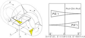


 , we prove a



1 Introduction
In 1963, E. Lorenz [Reference Lorenz45] introduced the following differential equations in the study of meteorology:
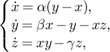 $$ \begin{align} \left\{ \begin{array}{@{}ll} \dot x=\alpha(y-x),\\ \dot y=\beta x-y-xz, \\ \dot z=xy-\gamma z, \end{array} \right. \end{align} $$
which has arisen much interest for dynamicists since then. For an open neighborhood of the chosen parameters
 $(\alpha ,\beta ,\gamma )=(10,28,8/3)$
, numerical simulations suggest that the system generated by the solution of (1.1) admits a strange attractor called the Lorenz attractor, which attracts almost all points in the phase space. Dynamics of Lorenz attractors behave in a chaotic way in the sense that it is transitive with dense periodic orbits, and thus, it is sensitively dependent on initial conditions. Although expressed in a simplified model, Lorenz equations (1.1) have been proved to be a challenge and present much difficulty for rigorous mathematical analysis. Thanks to the independent pioneering works of J. Guckenheimer [Reference Guckenheimer32] and V. Afra
 movi
 $\check {\mathrm { c}}$
-V. Bykov-L. Sil’nikov [Reference Afraĭmovič, Bykov and ’nikov2], a geometric model of a Lorenz attractor was introduced whose dynamics admits the behaviors observed by Lorenz. The geometric Lorenz attractor (see Definition 2.4) is defined through a three-dimensional smooth vector field and is proved to possess a singularity (or an equilibrium) which is robustly accumulated by regular orbits. However, the geometric Lorenz attractor is not structurally stable [Reference Guckenheimer32]. Works of J. Guckenheimer and R. Williams [Reference Guckenheimer and Williams33, Reference Williams74] gave good descriptions of the structure of geometric Lorenz attractors, which led more studies. W. Tucker [Reference Tucker69, Reference Tucker70] proved that the system generated from Lorenz original equations 1.1 admits the geometric model, which answers affirmatively [Reference Smale68, Problem 14] raised by S. Smale. Due to the existence of the singularity, the geometric Lorenz attractor is not hyperbolic (see Definition 2.1). To describe its geometric structure, C. Morales-M. Pacifico-E. Pujals [Reference Morales, Pacifico and Pujals52] introduced the notion of singular hyperbolicity (or sectional hyperbolicity); see Definition 2.2. One can refer to [Reference Li, Gan and Wen41, Reference Metzger and Morales49] for higher dimensions. S. Luzzatto-I. Melbourne-F. Paccaut [Reference Luzzatto, Melbourne and Paccaut46] proved the geometric Lorenz attractor is mixing with respect to its physical measure. More recently, V. Araújo-I. Melbourne [Reference Araújo and Melbourne3] proved some more properties including the existence of SRB measures, the central limit theorem and associated invariance principles.
In this paper, we prove a  connecting lemma for the geometric Lorenz attractor and study its ergodic measure space as an application. Perturbation theory plays a key role in the study of ‘most’ dynamical systems – for instance, in the exploration of
 $C^1$
-stability conjecture. C. Pugh’s closing lemma [Reference Pugh56] serves as a foundation of
 $C^1$
-perturbation theory. A series of important
 $C^1$
-perturbation theorems was inspired by this milestone work: the
 $C^1$
-closing lemma for conservative and Hamiltonian diffeomorphisms by C. Pugh-C. Robinson [Reference Pugh and Robinson57], the
 $C^1$
-ergodic closing lemma by R. Mañé [Reference Mañé47], the
 $C^1$
-closing lemma for nonsingular endomorphisms by L. Wen [Reference Wen71], the
 $C^1$
-connecting lemma by S. Hayashi [Reference Hayashi35]; see also M. Arnaud [Reference Arnaud6], L. Wen-Z. Xia [Reference Wen and Xia73]. The strongest
 $C^1$
-perturbation theorem would be the
 $C^1$
-chain connecting lemma which was proved by C. Bonatti-S. Crovisier [Reference Bonatti and Crovisier12]; see also [Reference Bonatti, Díaz and Viana15, Reference Crovisier21, Reference Crovisier22] for more applications. The proofs of these
 $C^1$
-perturbation theorems rely on local perturbation methods introduced by C. Pugh.
Compared to the completed perturbation theory in
 $C^1$
-topology, when
 $r\geq 2$
, the
 $C^r$
-perturbation theory is far from being accomplished. The
 $C^r (r\geq 2)$
perturbation problem turns out to be much more delicate and difficult. C. Gutierrez [Reference Gutierrez34] built an example which showed that C. Pugh’s local perturbation method for
 $C^1$
-perturbations does not work for
 $C^r (r\geq 2)$
case. When r is large, the
 $C^r$
-closing lemma is false for the system of Hamiltonian vector field constructed by M. Herman [Reference Herman36, Reference Herman37]. These two counterexamples imply that in general, global perturbations are needed in exploring the
 $C^r (r\geq 2)$
-perturbation problems. The lack of
 $C^r$
-perturbation techniques makes the study of
 $C^r$
-‘most’ dynamics be much difficult. For instance, the
 $C^r$
-stability conjecture is still widely open, for which one can refer to the survey by E. Pujals [Reference Pujals61]. For lower-dimensional dynamical systems, L-S. Young [Reference Young77] proved the
 $C^r$
-closing lemma for interval endomorphisms. M. Asaoka-K. Irie [Reference Asaoka and Irie7] proved a
 -closing lemma for Hamiltonian surface diffeomorphisms. In particular, S. Crovisier-E. Pujals [Reference Crovisier and Pujals24] proved the
 -closing lemma on the support of every ergodic measure for strongly dissipative surface diffeomorphisms, including a large class of Hénon maps. For higher-dimensional dynamical systems, R. Mañé [Reference Mañé48] proved a
 $C^2$
-connecting lemma to create homoclinic points under certain assumptions in the measure sense. Very recently, S. Gan and the first author [Reference Gan and Shi29] proved the
 $C^r$
-closing lemma for partially hyperbolic diffeomorphisms with 1-dimensional center.
Let
 $M^d$
(or M for simplicity) be a d-dimensional (
 $d\geq 3$
)
 smooth closed Riemannian manifold. For every
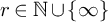 , we denote by
 $\mathscr {X}^r(M)$
the set of
 $C^r$
-smooth vector fields on M endowed with
 $C^r$
-topology. Given a vector field
 , we denote by
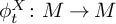 $\phi _t^X\colon M\rightarrow M$
the
 $C^r$
-flow generated by X and by
 $\Phi _t^X=D\phi _t^X$
the tangent map of
 $\phi _t^X$
. When there is no confusion, we also denote them by
 $\phi _t$
and
 $\Phi _t$
for simplicity. We denote by
 $\operatorname {Sing}(X)$
and
 $\operatorname {Per}(X)$
, respectively, the set of singularities and periodic points respectively of X. A point p is a critical element of X if
 . Our Theorem A is a
 $C^r$
-connecting lemma for geometric Lorenz attractors which creates homo/heteroclinic orbits associated to the singularity with a critical element (the singularity itself or a hyperbolic periodic orbit).
Theorem A. Let  and
 , which exhibits a geometric Lorenz attractor
 $\Lambda $
with singularity
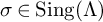 . Assume
 and
 is a critical element. Then there exists
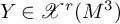 which is arbitrarily
 $C^r$
-close to X, such that
 $$ \begin{align*} \operatorname{Orb}(z,\phi_t^Y)\subseteq W^u(\sigma,\phi_t^Y)\cap W^s(p,\phi_t^Y), \end{align*} $$
with
 $\operatorname {Orb}(\sigma ,\phi _t^X)=\operatorname {Orb}(\sigma ,\phi _t^Y)$
and
 $\operatorname {Orb}(p,\phi _t^X)=\operatorname {Orb}(p,\phi _t^Y)$
.
Remark 1.1. (1) A more detailed statement of Theorem A is Theorem 3.10. The definition (Definition 2.4) of geometric Lorenz attractor follows J. Guckenheimer and R. Williams [Reference Guckenheimer32, Reference Guckenheimer and Williams33, Reference Williams74], since our Theorem A (& Theorem 3.10) requires that the reducing 1-dimensional map has derivative larger than
 $\sqrt {2}$
. Following this definition, we show that the vector fields exhibiting a geometric Lorenz attractor are an open subset of
 $\mathscr {X}^r(M^3)$
for every
 $r\geq 2$
; see Proposition 3.8.
(2) In the proof of Theorem A & 3.10, we apply a beautiful observation by [Reference Araújo and Melbourne3], which shows that the induced stable foliation of geometric Lorenz attractors in the cross section is
 $C^1$
-smooth. Moreover, we prove derivatives of holonomy maps of the induced stable foliations vary continuously with respect to vector fields in
 $C^2$
-topology. This implies the vector fields exhibiting a geometric Lorenz attractor forms a
 $C^2$
-open subset in
 $\mathscr {X}^r(M^3)$
for every
 ; see Appendix A.
(3) The critical element p in Theorem A can be
 $\sigma $
itself or a periodic point. Theorem A shows that for geometric Lorenz attractors, a homoclinic or heteroclinic orbit associate to the singularity can be generated through a
 $C^r$
-perturbation. It has its own interest in the study of homoclinic bifurcations for geometric Lorenz attractors. For instance, we show that
 $C^r$
-densely, the singularity inside a geometric Lorenz attractor. admits a homoclinic orbit (Corollary 3.11).
1.1 The space of ergodic measures on Lorenz attractors
As an application of Theorem A, we study the space of invariant measures supported on geometric Lorenz attractors of  where
 . This is motivated by the classical works of K. Sigmund [Reference Sigmund64, Reference Sigmund65, Reference Sigmund66] on the invariant measure space of basic sets for Axiom A systems [Reference Smale67] together with R. Mañé’s ergodic closing lemma [Reference Mañé47]. Given
 and an invariant compact set
 $\Lambda $
of
 $\phi _t^X$
, denote by
 $\mathcal {M}_{inv}(\Lambda )$
and
 $\mathcal {M}_{erg}(\Lambda )$
the spaces of invariant measures and ergodic measures respectively of X supported on
 $\Lambda $
endowed with the weak*-topology. Denote by
 $\mathcal {M}_{per}(\Lambda )$
the set of periodic measures (the invariant measure equidistributed on a single periodic orbit) supported on
 $\Lambda $
.
Recall that a basic set of an Axiom A diffeomorphism is a hyperbolic horseshoe which is topologically conjugate to a full shift, and in the case of Axiom A vector fields, a basic set
 $\Lambda $
is the suspension of a hyperbolic horseshoe
 $\Lambda '$
with a continuous roof function. Moreover, every basic set is a homoclinic class, where for a hyperbolic periodic point p, its homoclinic class
 $H(p)$
is the closure of the set of periodic points q homoclinically related to p (i.e.,
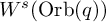 $W^s(\operatorname {Orb}(q))$
has nonempty transverse intersections with
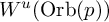 $W^u(\operatorname {Orb}(p))$
and vice versa). When
 $\Lambda $
is a basic set of an Axiom A system (diffeomorphism or vector field), K. Sigmund [Reference Sigmund64, Reference Sigmund65] proved that
 $\mathcal {M}_{per}(\Lambda )$
is dense in
 $\mathcal {M}_{inv}(\Lambda )$
and the set of ergodic measures with zero entropy forms a residual subset (i.e., a dense
 $G_\delta $
subset) of
 $\mathcal {M}_{inv}(\Lambda )$
. Another work of K. Sigmund [Reference Sigmund66] shows that the space of ergodic measures over a basic set of a diffeomorphism is path connected (or arcwise connected). For Axiom A vector fields, since a basic set
 $\Lambda $
is the suspension of a hyperbolic horseshoe
 $\Lambda '$
with a continuous roof function, thus by the one-to-one correspondence between invariant measures over
 $\Lambda $
and
 $\Lambda '$
(see, for instance, [Reference Parry and Pollicott54]), one has that
 $\mathcal {M}_{erg(\Lambda )}$
is also path connected. More statistical properties of periodic measures on basic sets are obtained by R. Bowen [Reference Bowen17, Reference Bowen18]. In the non-hyperbolic case, a recent work of A. Gorodetski-Y. Pesin [Reference Gorodetski and Pesin31] proves that if an isolated homoclinic class
 $H(p)$
of a diffeomorphism satisfies that all hyperbolic periodic orbits in
 $H(p)$
of the same index with p are homoclinically related with each other, then
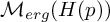 $\mathcal {M}_{erg}(H(p))$
is path connected. This gives a criterion for path connectedness of the ergodic measure space restricted on homoclinic classes. Other results on connectedness and topological properties of the invariant measure space for certain systems can be found in [Reference Bochi, Bonatti and Gelfert9, Reference Gelfert and Kwietniak30].
Every geometric Lorenz attractor is a homoclinic class in which all periodic orbits are homoclinically related (see Proposition 3.8), which is similar as basic sets and the isolated homoclinic class where A. Gorodetski-Y. Pesin [Reference Gorodetski and Pesin31] consider. However, due to the existence of the singularity, the ergodic measure space of a geometric Lorenz attractor may display a quite different nature. We show that for
 $C^r(r\geq 2)$
-dense vector fields
 admitting a geometric Lorenz attractor
 $\Lambda $
, the singular measure
 $\delta _\sigma $
is isolated in the space of ergodic measures
 $\mathcal {M}_{erg}(\Lambda )$
which breaks the connectedness of
 $\mathcal {M}_{erg}(\Lambda )$
. The key point is by applying Theorem A to make the two branches of the unstable manifold of
 $\sigma $
lie on the stable manifold of a periodic orbit
 $\operatorname {Orb}(p)$
through
 $C^r$
-perturbation. Then a criterion for isolated ergodic measures (Proposition 4.5) that we will prove ensures that the singular measure of the target system is isolated.
Meanwhile, as a sharp comparison of the above dense part, we prove that the denseness of periodic measures inside the space of invariant measures and the path connectedness of the ergodic measure space hold for geometric Lorenz attractors of
 $C^r$
-generic
 (i.e., vector fields in a residual (dense
 $G_\delta $
)subset of
 $\mathscr {X}^r(M^3)$
), which proves [Reference Bonatti11, Conjecture 2] for geometric Lorenz attractors in
 $C^r(r\geq 2)$
-topology. This is in spirit of Sigmund’s work [Reference Sigmund64, Reference Sigmund65, Reference Sigmund66] mentioned above and R. Mañé’s ergodic closing lemma [Reference Mañé47]. The ergodic closing lemma is a milestone in dynamical systems and ergodic theory, and it plays a key role in solving the stability conjecture. A classical consequence of the ergodic closing lemma is that for
 $C^1$
-generic diffeomorphisms or vector fields, the set of periodic measures and singular measures are dense in the space of ergodic measures. However, things become more complicated to verify the denseness of periodic measures in the space of ergodic measures when restricted to a non-hyperbolic compact invariant set
 $\Lambda $
. The difficulty is how to guarantee that the periodic measures (maybe obtained by perturbations) provided by the ergodic closing lemma are contained in
 $\Lambda $
; see, for instance, C. Bonatti’s survey [Reference Bonatti11, Conjecture 2]. Progresses and some important criterion can be found in the work of F. Abdenur-C. Bonatti-S. Crovisier [Reference Abdenur, Bonatti and Crovisier1]. Other works on the approximation of invariant measures by periodic ones can be found in [Reference Bomfim, Torres and Varandas10, Reference Bonatti and Zhang16, Reference Díaz, Gelfert, Marcarini and Rams28, Reference Hirayama38, Reference Liang, Liu and Sun42, Reference Yang and Zhang75].
In sum, our Theorem B gives a sharp contrast on ergodic measure space for geometric Lorenz attractors between
 $C^r (r\geq 2)$
-dense and
 $C^r$
-generic vector fields in
 $\mathscr {X}^r(M^3)$
.
Theorem B. For every  , there exist a dense subset
 $\mathscr {D}^r\subset \mathscr {X}^r(M^3)$
and a residual subset
 $\mathscr {R}^r\subset \mathscr {X}^r(M^3)$
, such that
-
• If
 $\Lambda $
is a geometric Lorenz attractor of , then
$\overline {\mathcal {M}_{per}(\Lambda )}\subsetneqq \overline {\mathcal {M}_{erg}(\Lambda )}\subsetneqq \mathcal {M}_{inv}(\Lambda )$
. Moreover, the space
$\mathcal {M}_{erg}(\Lambda )$
is not connected.
-
• If
$\Lambda $
is a geometric Lorenz attractor of , then
$\overline {\mathcal {M}_{per}(\Lambda )}= \overline {\mathcal {M}_{erg}(\Lambda )}= \mathcal {M}_{inv}(\Lambda )$
. Moreover, the space
$\mathcal {M}_{erg}(\Lambda )$
is path connected.

 , then



 , then


Remark 1.2. Recall that the geometric Lorenz attractor is a homoclinic class; see Proposition 3.8. To the authors’ knowledge, the dense part of Theorem B (together with Theorem B.1 in Appendix B) is the first known example of locally dense systems (in any
 $C^r$
-topology where
 $r\geq 1$
) exhibiting an isolated ergodic measure supported on a homoclinic class.
Remark 1.3. In our construction for the dense part of Theorem B, the atomic measure
 $\delta _{\sigma }$
of the singularity
 $\sigma $
is isolated in the ergodic measure space. We kick the atomic measure
 $\delta _{\sigma }$
out in the same spirit of [Reference Bonatti, Crovisier, Gourmelon and Potrie13], where the authors kick out a single orbit of a chain recurrence class from a homoclinic class. Actually, for every geometric Lorenz attractor
 $\Lambda $
, let
 $\mathcal {M}_0=\mathcal {M}_{erg}(\Lambda )\setminus \{\delta _{\sigma }\}$
and
 . Then
 $\mathcal {M}_0$
is path connected, and moreover,
 $\overline {\mathcal {M}_{per}(\Lambda )}=\overline {\mathit {Convex}(\mathcal {M}_0)}=\overline {\mathcal {M}_1}$
. Here,
 $\mathit {Convex}(\mathcal {M}_0)$
consists all elements that are convex combinations of measures in
 $\mathcal {M}_0$
.
The following corollary of Theorem B concerns the support and entropy of invariant measures for
 $C^r(r\geq 2)$
-generic geometric Lorenz attractors.
Corollary 1.4. For every  , there exists a residual subset
 $\mathscr {R}^r\subset \mathscr {X}^r(M^3)$
, such that for every
 , if
 $\Lambda $
is a geometric Lorenz attractor of X, then
-
• there exists a residual subset
$\mathcal {M}_{res}$
in
$\mathcal {M}_{inv}(\Lambda )$
such that every is ergodic with
$\operatorname {Supp}(\mu )=\Lambda $
and
$h_{\mu }=0$
. -
• there exists a dense subset
$\mathcal {M}_{den}$
in
$\mathcal {M}_{inv}(\Lambda )$
such that every is ergodic with
$h_{\mu }>0$
.


 is ergodic with



 is ergodic with

Remark 1.5. For every geometric Lorenz attractor
 $\Lambda $
of every
 , the measures with zero entropy and full support form a residual subset in
 $\mathcal {M}_{inv}(\Lambda )$
. See Remark 4.16.

Organization of the paper
In Section 2, we state some preliminaries on singular hyperbolicity and geometric Lorenz attractors. The proof of Theorem A together with a detailed characterization of geometric Lorenz attractors is given in Section 3. Then we study the ergodic measure space of geometric Lorenz attractors and prove Theorem B together with Corollary 1.4 in Section 4. In Appendix A, we give a proof of Proposition 3.8, which states that the
 $C^r(r\geq 2)$
-vector fields admitting a geometric Lorenz attractor forms an open subset of
 $\mathscr {X}^r(M)$
. In Appendix B, we sketch some conclusions concerning ergodic measure spaces of singular hyperbolic attractors for
 $C^1$
vector fields of any dimension.
2 Preliminary
Recall that for a
 $C^r(r\geq 1)$
-vector field
 , we denote by
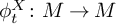 $\phi _t^X\colon M\rightarrow M$
the
 $C^r$
-flow generated by X and by
 $\Phi _t^X=D\phi _t^X$
the tangent map of
 $\phi _t^X$
. We also use
 $\phi _t$
and
 $\Phi _t$
for simplicity if there is no confusion.
2.1 Singular hyperbolicity
We give the definition of hyperbolic and singular hyperbolic set.
Definition 2.1. Given a vector field 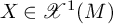 . An invariant compact set
 $\Lambda $
is hyperbolic if
 $\Lambda $
admits a continuous
 $\Phi _t$
-invariant splitting
 $T_{\Lambda }M=E^s\oplus \langle X\rangle \oplus E^u$
, where
 $\langle X\rangle $
denotes the one-dimensional linear space generated by the flow direction, such that
 $E^s$
is contracted by
 $\Phi _t$
and
 $E^u$
is expanded by
 $\Phi _t$
. To be precise, there exist two constants
 $C>0$
and
 $\eta>0$
, such that for any
 and any
 $t\geq 0$
, it satisfies the following:
-
• for any
,
$\|\Phi _t(v)\|\leq Ce^{-\eta t}\|v\|$
; -
• for any
,
$\|\Phi _{-t}(v)\|\leq Ce^{-\eta t}\|v\|$
.
 ,

 ,

The stable dimension
 $\dim (E^s)$
is called the index of the hyperbolic splitting.
The notion of singular hyperbolicity was introduced by Morales-Pacifico-Pujals [Reference Morales, Pacifico and Pujals52] to describe the geometric structure of Lorenz attractors and was then developed in higher dimensions by [Reference Li, Gan and Wen41, Reference Metzger and Morales49]. It is proved in [Reference Morales, Pacifico and Pujals52] that any robustly transitive set of a three-dimensional vector field is singular hyperbolic, and a similar conclusion holds for higher dimensions [Reference Li, Gan and Wen41, Reference Zhu, Gan and Wen78]. We refer to [Reference Araújo and Pacifico4] for a comprehensive introduction of singular hyperbolic vector fields.
Definition 2.2. Given a vector field 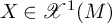 . An invariant compact set
 $\Lambda $
is singular hyperbolic if
 $\Lambda $
admits a continuous
 $\Phi _t$
-invariant splitting
 $T_{\Lambda }M=E^{ss}\oplus E^{cu}$
and there exist two constants
 $C,\eta>0$
, such that for any
 and any
 $t\geq 0$
, it satisfies the following:
-
•
$E^{ss}\oplus E^{cu}$
is a dominated splitting:
$\|\Phi _t|_{E^{ss}(x)}\|\cdot \|\Phi _{-t}|_{E^{cu}(\phi _t(x))}\|< Ce^{-\eta t}$
; -
•
$E^{ss}$
is contracted by
$\Phi _t$
:
$\|\Phi _t(v)\|< Ce^{-\eta t}$
for any ; -
•
$E^{cu}$
is sectionally expanded by
$\Phi _t$
:
$\|\det \Phi _t(x)|_{V_x}\|> Ce^{\eta t}$
for any 2-dimensional subspace
$V_x\subset E^{cu}_x$
.





 ;




Remark 2.3. (1) Given 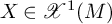 . If an invariant compact set
 $\Lambda $
is hyperbolic, then
 $\Lambda $
must contain no singularity. However, if
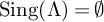 $\operatorname {Sing}(\Lambda )=\emptyset $
, then
 $\Lambda $
is hyperbolic if and only if
 $\Lambda $
is singular hyperbolic for X or for
 $-X$
.
(2) By definition, singular hyperbolicity is a robust property. To be precise, if
 $\Lambda $
is a singular hyperbolic invariant compact set of
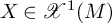 associated with splitting
 $T_{\Lambda }M=E^{ss}\oplus E^{cu}$
and constants
 $(C,\eta )$
, then there exist a neighborhood U of
 $\Lambda $
and a neighborhood
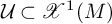 $\mathcal {U}\subset \mathscr {X}^1(M)$
of X such that for any
 , the maximal invariant set of
 $\phi _t^Y$
in U is singular hyperbolic associated with the same stable dimension and constants
 $(C,\eta )$
.
2.2 The geometric Lorenz attractor
We follow the constructions of Guckenheimer and Williams [Reference Guckenheimer32, Reference Guckenheimer and Williams33, Reference Williams74] to give the definition of geometric Lorenz attractor for any
 $C^r (r\geq 1)$
vector field. Let
 where
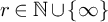 , an open subset
 $U\subseteq M$
is called an attracting region of X, if for every
 , the vector field
 $X(x)$
is transverse to
 $\partial U$
and points to the interior of U, and
 for every
 $t>0$
. This implies
 $\overline {\phi _t^X(U)}=\phi _t^X(\overline {U})\subsetneqq U$
for every
 $t>0$
. An invariant compact set
 $\Lambda $
is an attractor of X if
 $\Lambda $
is transitive and
 $\Lambda $
is the maximal invariant set of an attracting region. Recall that
 $M^3$
denotes a three-dimensional closed smooth Riemannian manifold.
Definition 2.4. Let
 $r\geq 2$
and
 . We say X admits a geometric Lorenz attractor
 $\Lambda $
if X has an attracting region
 $U\subset M^3$
such that
 $\Lambda =\bigcap _{t>0}\phi ^X_t(U)$
is a singular hyperbolic attractor and satisfies the following properties:
-
•
$\Lambda $
contains a unique singularity
$\sigma $
with three eigenvalues
$\lambda _1<\lambda _2<0<\lambda _3$
with respect to
$\Phi _1(\sigma )$
satisfying
$\lambda _1+\lambda _3<0$
and
$\lambda _2+\lambda _3>0$
. -
•
$\Lambda $
admits a
$C^r$
-smooth cross section
$\Sigma $
which is
$C^1$
-diffeomorphic to
$[-1,1]\times [-1,1]$
, such that for every , there exists
$t>0$
such that , and
$l=\{0\}\times [-1,1]=W^s_{\mathit {loc}}(\sigma )\cap \Sigma $
. -
• The Poincaré map
$P:\Sigma \setminus l\rightarrow \Sigma $
is
$C^1$
-smooth in the coordinate
$\Sigma =[-1,1]^2$
and has the form
$P(x,y)=\big ( f(x)~,~H(x,y) \big )$
for every . Moreover, it satisfies-
–
$H(x,y)<0$
for
$x>0$
,
$H(x,y)>0$
for
$x<0$
, and , ; -
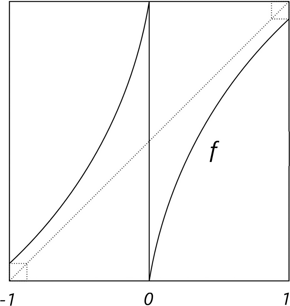
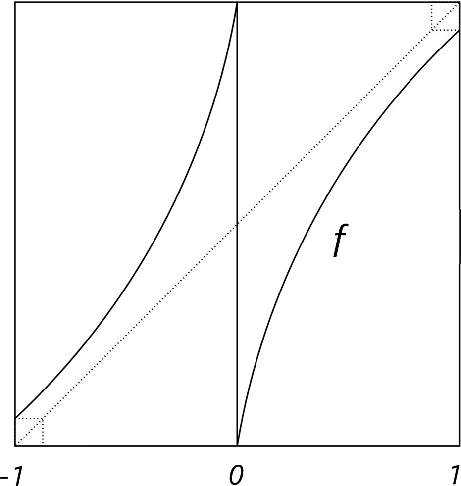
– the one-dimensional quotient map
$f:[-1,1]\setminus \{0\}\rightarrow [-1,1]$
is
$C^1$
-smooth and satisfies
$\lim _{x\rightarrow 0^-}f(x)=1$
,
$\lim _{x\rightarrow 0^+}f(x)=-1$
,
$-1<f(x)<1$
and
$f'(x)>\sqrt {2}$
for every (see Figure 2 below).
-






 , there exists

 , and



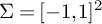

 . Moreover, it satisfies


 ,
 ;






 (see Figure
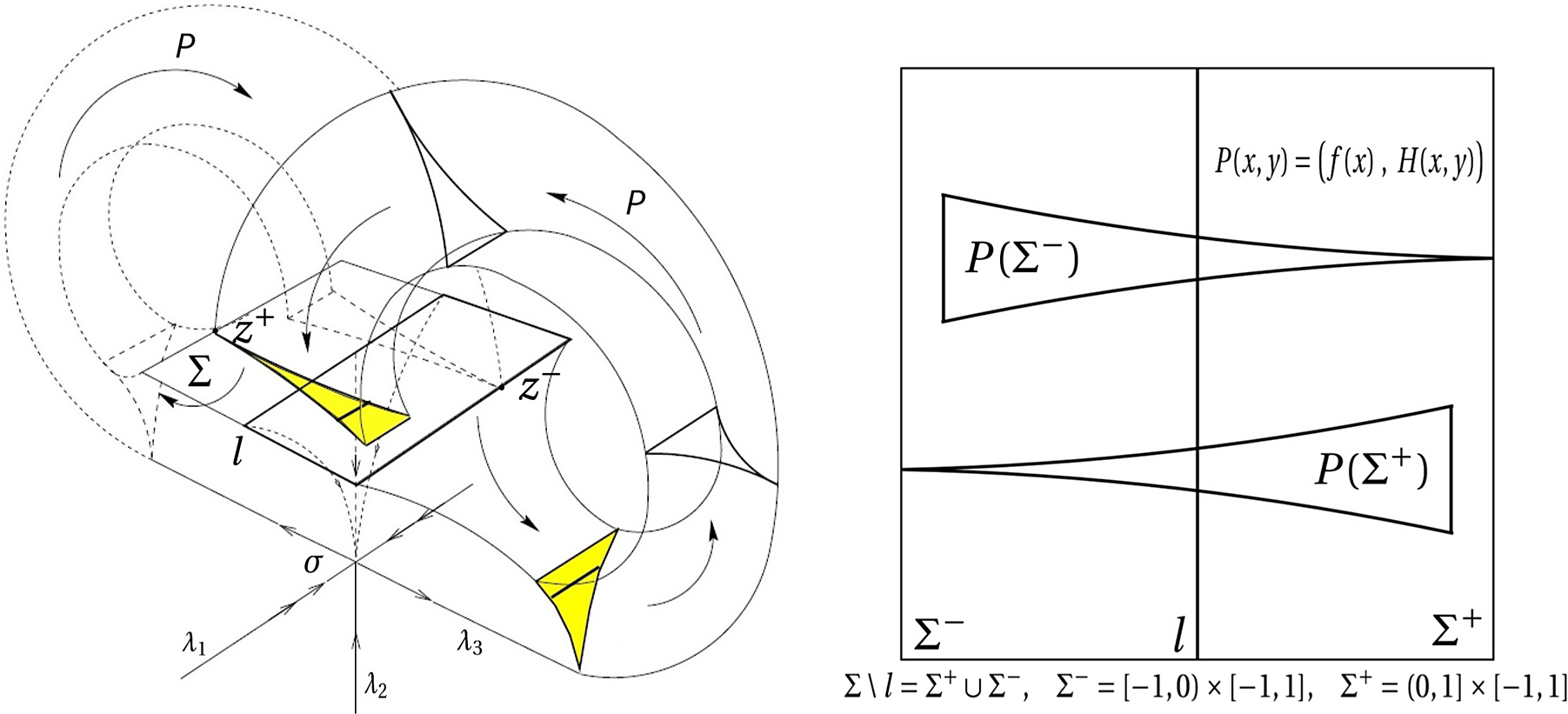
Remark 2.5. The unstable manifold of
 $\sigma $
contains two orbits. We denote
 which satisfy
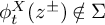 $\phi _t^X(z^{\pm })\notin \Sigma $
for every
 $t<0$
(see Figure 1), and

Here, we can assume
 $-1<y^+<0$
and
 $0<y^-<1$
by changing the y-coordinate. For every
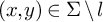 , if
 $x\rightarrow 0^+$
, then
 $P(x,y)$
approaches
 $z^+$
; if
 $x\rightarrow 0^-$
, then
 $P(x,y)$
approaches
 $z^-$
.
Geometric Lorenz attractor and return map.
The Lorenz expanding map.
Lemma 2.6. The Poincaré map
 $P(x,y)=\big ( f(x),H(x,y) \big ):\Sigma \setminus l\rightarrow \Sigma $
satisfies

Moreover, for every
 $\alpha>0$
, let the cone field
 be defined on
 $\Sigma $
as
 $$ \begin{align*} \mathcal{C}_{\alpha}(x,y)~=~\big\{v=a\cdot\partial/\partial x +b\cdot\partial/\partial y:~ |b|\leq\alpha\cdot |a|\big\}. \end{align*} $$
Then for every
 $\alpha \geq 1/(\sqrt {2}-1)$
, the Poincaré map P satisfies

Proof. Since
 $(x,y)\rightarrow W^s_{\mathit {loc}}(\sigma )$
as
 $x\rightarrow 0$
, the orbit of
 $(x,y)$
approaches the singularity
 $\sigma $
. As we assumed
 $\lambda _1<\lambda _2<0$
and
 $\lambda _2+\lambda _3>0$
; thus,
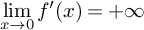 and
 $\lim \limits _{x\rightarrow 0}\big |\partial H(x,y)/\partial y\big |=0$
. Moreover, for every
 $\alpha \geq 1/(\sqrt {2}-1)$
and
 , if we denote
 $DP(v)=a\cdot \partial /\partial x+b\cdot \partial /\partial y$
, then we have
 $|a|>\sqrt {2}$
and
 $|b|\leq 1+\alpha \leq \alpha \cdot \sqrt {2}$
. This implies
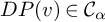 .
Remark 2.7. For every point  , the cone field
 $\mathcal {C}_{\alpha }(z)\oplus \left \langle X(z)\right \rangle $
is a neighborhood of center-unstable bundle
 $E^{cu}(z)$
of z.
In Definition 2.4, the property  is not necessary. We only need that there exists some constant
 $K>0$
, such that
 , which automatically holds because
 $\Lambda $
is singular hyperbolic and H is uniformly
 $C^1$
-smooth. Then we can take
 $\alpha \geq K/(\sqrt {2}-1)$
, and the cone field
 $\mathcal {C}_{\alpha }$
is
 $DP$
-invariant.
It has been showed in [Reference Carmona, Carrasco-Olivera and San Martín20] that, following Definition 2.4, every geometric Lorenz attractor
 $\Lambda $
is robustly transitive. In Section 3, we will introduce a series of properties of geometric Lorenz attractors. In particular, the
 $C^r$
-vector fields exhibiting a geometric Lorenz attractor consists an open subset in
 $\mathscr {X}^r(M^3)$
for every
 $r\geq 2$
(Proposition 3.8).
3 A
$C^r$
-connecting lemma of the geometric Lorenz attractors

In this section, we give the proof of Theorem A. The more detailed statement is Theorem 3.10 below. Before the proof, we first state some basic properties of geometric Lorenz attractors in the following subsection.
3.1 Properties of geometric Lorenz attractors
In this subsection, we investigate some properties for the geometric Lorenz attractor. We assume  and
 , which exhibits a geometric Lorenz attractor
 $\Lambda $
with cross section
 $\Sigma $
. Let
 $P(x,y)=\big (f(x),H(x,y)\big ):\Sigma \setminus l\rightarrow \Sigma $
be the Poincaré map of
 $\phi _t^X$
.
Recall that
 $\Lambda $
is a singular hyperbolic attractor with splitting
 $T_{\Lambda }M^3=E^{ss}\oplus E^{cu}$
and there exists a Hölder continuous foliation
 $\mathcal {F}^{ss}$
tangent to
 $E^{ss}$
everywhere [Reference Pugh, Shub and Wilkinson60]. Since the strong stable bundle
 $E^{ss}$
is determined by the positive orbit of a point and
 $\Lambda $
is an attractor,
 $E^{ss}$
and
 $\mathcal {F}^{ss}$
is well defined in the whole attracting region U. Moreover, we have the following lemma.
Lemma 3.1. For every  , if we define

then
 $\mathcal {F}^s$
is a 2-dimensional
 $\phi _t^X$
-invariant foliation in
 $U\setminus \mathcal {F}^{ss}(\sigma )$
. Moreover, each leaf of
 $\mathcal {F}^s$
is
 $C^r$
-smooth, and the holonomy map of
 $\mathcal {F}^s$
is
 $C^{1}$
-smooth.
Proof. The definition of
 $\mathcal {F}^s$
implies it is a 2-dimensional
 $\phi _t^X$
-invariant foliation in
 $U\setminus \mathcal {F}^{ss}(\sigma )$
. The classical invariant manifold theorem [Reference Hirsch, Pugh and Shub39] shows each leaf of
 $\mathcal {F}^{ss}$
is
 $C^r$
-smooth, and so is each leaf of
 $\mathcal {F}^s$
. The fact that holonomy maps of
 $\mathcal {F}^s$
are
 $C^{1}$
-smoothFootnote
1
has been proved in [Reference Araújo and Melbourne3, Lemma 7.1].
Lemma 3.2. There exists a
 $C^r$
-smooth cross section
 $\Sigma _1$
of
 $\phi _t^X$
which is an extension of
 $\Sigma $
and
 $C^1$
-diffeomorphic to
 $[-1-\epsilon ,1+\epsilon ]^2$
for some
 $\epsilon>0$
such that
 $$ \begin{align*} l_1=\{0\}\times[-1-\epsilon,1+\epsilon] =\Sigma_1\cap W^s_{\mathit{loc}}(\sigma,\phi_t^X), \quad \mathrm{and} \quad \Sigma=[-1,1]^2\subset [-1-\epsilon,1+\epsilon]^2=\Sigma_1. \end{align*} $$
The Poincaré map
 $P:\Sigma \setminus l\rightarrow \Sigma $
smoothly extends to a Poincaré map
 $P_1:\Sigma _1\setminus l_1\rightarrow \Sigma _1$
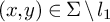
, which has the form
 $P_1(x,y)=\big ( f_1(x), H_1(x,y) \big )$
for every
 and satisfies
 $P_1|_{\Sigma \setminus l}\equiv P$
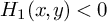
. Moreover, they satisfy the following:
-
•
$H_1(x,y)>0$
for
$x>0$
,
$H_1(x,y)<0$
for
$x<0$
, and , ; -
• the one-dimensional quotient map
$f_1:[-1-\epsilon ,1+\epsilon ]\setminus \{0\}\rightarrow [-1,1]$
is
$C^1$
-smooth and satisfies
$f_1|_{[-1,1]\setminus \{0\}}\equiv f$
,
$-1<f(x)<1$
and
$f'(x)>\sqrt {2}$
for every .
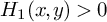


 ,
 ;





 .
In particular, the image of the Poincaré map
 $P_1$
satisfies
 $\overline {P_1(\Sigma _1\setminus l_1)} \subseteq [-1,1]\times (-1,1)$
.
Remark 3.3. Here, even the cross section
 $\Sigma _1$
is
 $C^r$
-smooth; the stable foliation
 $\mathcal {F}^s\cap \Sigma _1$
induced by the flow intersecting with
 $\Sigma _1$
can only be
 $C^1$
but not
 $C^r$
-smooth. If we want to take a coordinate
 $[-1-\epsilon ,1+\epsilon ]^2$
where
 $x\times [-1-\epsilon ,1+\epsilon ]$
is the leaf of induced stable foliations
 $\mathcal {F}^s\cap \Sigma _1$
, this coordinate can only be
 $C^1$
-smooth. This is why we say
 $\Sigma _1$
is
 $C^1$
-diffeomorphic to
 $[-1-\epsilon ,1+\epsilon ]^2$
in the lemma.
Proof. Since
 $\Sigma $
is a
 $C^r$
-smooth cross section of
 $\phi _t^X$
, we can extend
 $\Sigma $
to a larger surface
 $\Sigma _1$
transverse to
 $\phi _t^X$
. Moreover, Lemma 3.1 shows that the stable foliation
 $\mathcal {F}^s$
intersects
 $\Sigma _1$
inducing a
 $C^{1}$
-smooth foliation in
 $\Sigma _1$
, where we already have
 . So we can
 $C^1$
-smoothly extend the coordinate of
 $\Sigma $
to
 $\Sigma _1=[-1-\epsilon ,1+\epsilon ]^2$
for some
 $\epsilon>0$
, such that

and
 $l_1=0\times [-1-\epsilon ,1+\epsilon ]=W^s_{\mathit {loc}}(\sigma ,\phi _t^X)\cap \Sigma _1$
.
Let
 $P_1:\Sigma _1\setminus l_1\rightarrow \Sigma _1$
be the Poincaré map associated to
 $\Sigma _1$
. Then it has the form
 $P_1(x,y)=(f_1(x), H_1(x,y))$
and
 $P_1|_{\Sigma \setminus l}\equiv P$
. In particular,
 $f_1$
is
 $C^1$
-smooth and
 $f_1|_{[-1,1]\setminus \{0\}}\equiv f$
. From the definition of geometric Lorenz map, the one-dimensional quotient map
 $f:[-1,1]\setminus \{0\}\rightarrow [-1,1]$
satisfies
 $-1<f(x)<1$
and
 $f'(x)>\sqrt {2}$
everywhere. This implies
 $-1<f(-1)<0<f(1)<1$
. Thus, if we choose
 $\epsilon $
small enough, we also have
 $-1<f_1(1-\epsilon )<0<f(1+\epsilon )<1$
. Shrinking
 $\epsilon $
if necessary,
 $P_1$
is well defined on
 $\Sigma _1\setminus l_1$
, and
 $H_1,f_1$
satisfies all estimations of
 $H,f$
. In particular, we have
 $$ \begin{align*} \overline{P_1(\Sigma_1\setminus l_1)}= P_1(\Sigma_1\setminus l_1)\cup\{z^+,z^-\} \subseteq[-1,1]\times(-1,1).\\[-34pt] \end{align*} $$
Notation 3.4. From now on, we use
 $\Sigma ,P,f,H$
to denote
 $\Sigma _1,P_1,f_1,H_1$
, respectively, for the simplicity of notations. We denote
 $\pi _x:\Sigma \rightarrow [-1-\epsilon ,1+\epsilon ]$
the projection to x-coordinate on
 $\Sigma $
. Since
 , there exists
 $\lambda _0>\sqrt {2}$
, such that
 $f'(x)>\lambda _0$
for every
 . However, since
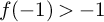 $f(-1)>-1$
, we must have
 $\lambda _0<2$
.
We fix
 $\alpha =1/(\sqrt {2}-1)$
. The proof of Lemma 2.6 shows that the cone field
 $\mathcal {C}_{\alpha }$
satisfies

Definition 3.5. Let
 $\mathscr {L}^r~(r\geq 1)$
be the set consisting of
 $C^r$
-maps
 $f:[-1,1]\setminus \{0\}\rightarrow (-1,1)$
which satisfies
-
•
$\lim _{x\rightarrow 0^-}f(x)=1$
, and ; -
•
$\lim _{x\rightarrow 0^+}f(x)=-1$
, and ; -
•
$-1<f(x)<1$
and there exists
$\lambda _0>\sqrt {2}$
such that
$f'(x)>\lambda _0$
for every .

 ;

 ;



 .
We call  a Lorenz expanding map.
The following lemma is standard in the study of geometric Lorenz attractors; see [Reference Williams74, Proposition 1]. We include a new proof which is more quantitative and illustrates the main idea of proving Claim 3.16 in the proof of Theorem 3.10.
Lemma 3.6. Let  . Then f is eventually onto – that is, for every open interval
 $J\subset [-1,1]\setminus \{0\}$
, there exists an integer
 $N>0$
, such that
 $\bigcup _{i=0}^Nf^i(J)=(-1,1)$
.
New proof of Lemma 3.6
For every
 $n\geq 1$
, we consider the map
 $f^n:J\rightarrow [-1,1]$
. Let

We call  a discontinuity point of
 $f^n$
. Then
 $D_n$
is a finite subset of J with
 $D_n\subseteq D_{n+1}$
, and
 $f^n$
is well defined and
 $C^1$
-smooth on each connected component of
 $J\setminus D_n$
. Moreover, if
 $(a,b)\subseteq J$
is a connected component of
 $J\setminus D_n$
, then
 $f^n|_{(a,b)}$
is a diffeomorphism from
 $(a,b)$
to its image

Claim 3.7. For every
 $n\geq 1$
, assume
 $I=(a,b)$
is a connected component of
 $J\setminus D_n$
. Then either
 $\#\big (I\cap D_{n+2}\big )\leq 1$
, or
 $(-1,1)\subseteq f^{n+1}(I)\cup f^{n+2}(I)$
.
Proof of the claim.
Recall that
 $f^n$
is well defined and
 $C^1$
-smooth on I. Let
 $(c,d)=f^n(I)$
. Since
 $I\cap D_n=\emptyset $
, one has that
 $f^m(t)\neq 0$
for any
 and
 $1\leq m\leq n-1$
by definition of
 $D_n$
. If
 $0\notin (c,d)$
, which means that
 $f^n(t)\neq 0$
for any
 , then one has
 $I\cap D_{n+1}=\emptyset $
by definition of
 $D_{n+1}$
. As a consequence,
 $f^{n+1}(I)=f(c,d)$
is an open interval in
 $(-1,1)$
. Thus, there exists at most one point
 , such that
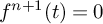 $f^{n+1}(t)=0$
. This implies
 $\#\big (I\cap D_{n+2}\big )\leq 1$
.
If, however,  , then we denote
 satisfying
 $f^n(t_0)=0$
. Then the two open intervals
 $(a,t_0)$
and
 $(t_0,b)$
are two connected components of
 $J\setminus D_{n+1}$
. Moreover, their images by
 $f^{n+1}$
satisfy
 $$ \begin{align*} f^{n+1}(a,t_0)=\big(\lim_{x\rightarrow a^+}f(x),~1\big), \qquad \mathrm{and } \qquad f^{n+1}(t_0,b)=\big(-1,~\lim_{x\rightarrow a^+}f(x)\big). \end{align*} $$
If neither of them contains
 $0$
, then we have
 $\#\big (I\cap D_{n+2}\big )=\#\big (I\cap D_{n+1}\big )=1$
.
Otherwise, we have either  or
 . Thus, either
 $$ \begin{align*} [0,1)\subset f^{n+1}(a,t_0)\subset f^{n+1}(I), \qquad \mathrm{or} \qquad (-1,0]\subset f^{n+1}(t_0,b)\subset f^{n+1}(I). \end{align*} $$
In both cases, iterating by f again, we have
 $(-1,1)\subseteq f^{n+1}(I)\cup f^{n+2}(I)$
.
Now we show that there exists some
 $n>0$
and a connected component I of
 $J\setminus D_n$
, such that
 $(-1,1)\subseteq f^{n+1}(I)\cup f^{n+2}(I)$
. Otherwise, Claim 3.7 implies
 $$ \begin{align*} \# D_2\leq1, \!\!\!\qquad \# D_4\leq\# D_2+\# D_2+1\leq 3, \!\!\qquad \cdots \!\!\qquad \# D_{2n}\leq \# D_{2n-2}+\# D_{2n-2}+1\leq 2^n-1. \end{align*} $$
This implies
 $J\setminus D_{2n}$
has at most
 $2^n$
connected components. So there exists a connected component
 $I_{2n}\subset J\setminus D_{2n}$
, such that its length satisfies
 $|I_{2n}|\geq 2^{-n}|J|$
.
Since f is a diffeomorphism on each connected component, and satisfies
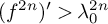 $(f^{2n})'>\lambda _0^{2n}$
, the length of the interval
 $f^{2n}(I_{2n})$
satisfies

This is absurd since
 $f^{2n}(I_{2n})\subseteq (-1,1)$
. We take
 $N=n+2$
finishing the proof of this lemma.
The following proposition shows that every Lorenz attractor is a homoclinic class and every pair of periodic orbits is homoclinic related. Moreover, for every  , the set of
 $C^r$
vector fields exhibiting a geometric Lorenz attractor is an open subset of
 $\mathscr {X}^r(M^3)$
.
Proposition 3.8. Let  and
 . If X exhibits a geometric Lorenz attractor
 $\Lambda $
with attracting region U, then
 $\Lambda $
is a singular hyperbolic homoclinic class of X, and the orbits of every two periodic points
 are homoclinic related.
Moreover, there exists a
 $C^r$
-neighborhood
 $\mathcal {U}$
of X in
 $\mathscr {X}^r(M^3)$
, such that for every
 , U is an attracting region of Y, and the maximal invariant set
 $\Lambda _Y=\bigcap _{t>0}\phi _t^Y(U)$
is a geometric Lorenz attractor.
Remark 3.9. The proof of Proposition 3.8 is in Appendix A. The first part is classical, and the ‘moreover’ part relies on a beautiful observation in [Reference Araújo and Melbourne3], which shows the stable foliation of the Poincaré map in the cross section is
 $C^{1+}$
-smooth.
3.2 A
$C^r$
-connecting theorem of geometric Lorenz attractors

This subsection is devoted to prove Theorem A, which is a
 $C^r$
-connecting theorem for geometric Lorenz attractors. One can see that Theorem A follows from the following technical one with more details.
Theorem 3.10 (Theorem A revisited).
Assume  and
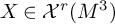 admits a geometric Lorenz attractor
 $\Lambda $
with singularity
 $\sigma $
and attracting region U. Let
 $\Sigma $
be the cross section of
 $\Lambda $
from Notation 3.4, and
 be a point satisfying
 $\phi _t^X(z)\notin \Sigma $
for every
 $t<0$
.
For every
 $C^r$
-neighborhood
 $\mathcal {V}$
of X, every critical element
 and every
 $\delta _0>0$
, there exist
 $0<\delta <\delta _0$
and
 , such that the maximal invariant set
 $\Lambda _Y=\bigcap _{t>0}\phi _t^Y(U)$
is a geometric Lorenz attractor satisfying the following:
-
1. The vector field Y and
$\delta $
-neighborhood
$B(z,\delta )$
of z satisfy This implies
$$ \begin{align*} Y|_{M^3\setminus B(z,\delta)}~\equiv~ X|_{M^3\setminus B(z,\delta)}, \qquad \mathit{and} \qquad B(z,\delta)~\cap~\left(\operatorname{Orb}(p,\phi_t^X)\cup\{\sigma\}\right) ~=~\emptyset. \end{align*} $$
, and with
$\operatorname {Orb}(p,\phi _t^Y)=\operatorname {Orb}(p,\phi _t^X)$
.
-
2. The point
and there exists
$T>0$
, such that . This implies
$$ \begin{align*} \operatorname{Orb}(z,\phi_t^Y)~\subset~ W^u(\sigma,\phi_t^Y) \cap W^s(\operatorname{Orb}(p),\phi_t^Y). \end{align*} $$



 , and
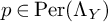 with

 and there exists

 . This implies

Before proving Theorem 3.10, we would like to state the following direct corollary by considering the critical element p as the singularity
 $\sigma $
itself, which shows that
 $C^r$
-densely, the singularity in the geometric Lorenz attractor admits a homoclinic orbit.
Corollary 3.11. Assume  . There exists a dense subset
 $\mathcal {D}^r_h\subset \mathscr {X}^r(M^3)$
, such that if
 admits a geometric Lorenz attractor with singularity
 $\sigma $
, then
 $\sigma $
has a homoclinic orbit.
Now we give the proof of Theorem 3.10.
Proof of Theorem 3.10.
By Proposition 3.8, we can shrink the
 $C^r$
-neighborhood
 $\mathcal {V}$
of X if necessary, such that for every
 , the maximal invariant set
 $\Lambda _Y=\bigcap _{t>0}\phi _t^Y(U)$
is a geometric Lorenz attractor.
There are two points  satisfying
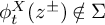 $\phi _t^X(z^\pm )\notin \Sigma $
for every
 $t<0$
. We assume
 . The proof for
 $z=z^-$
is the same.
For the critical element  , there are two possibilities: either
 $p=\sigma $
or p is a periodic point.
-
• If
$p=\sigma $
, there exists , such that
$B(z,\delta )\cap W^s_{\mathit {loc}}(\sigma )=\emptyset $
. We only need to show there exists a vector field which satisfies
$Y|_{M^3\setminus B(z,\delta )}~\equiv ~ X|_{M^3\setminus B(z,\delta )}$
, such that for some
$T>0$
, -
• If p is a periodic point, then we can assume
with There exists, such that
$B(z,\delta )\cap \left (\bigcup _{t\geq 0}\phi _t^X(l_p)\cup \{\sigma \}\right ) =\emptyset $
. We need to show there exists a vector field which satisfies
$Y|_{M^3\setminus B(z,\delta )}~\equiv ~ X|_{M^3\setminus B(z,\delta )}$
, such that for some
$T>0$
,

 , such that

 which satisfies



 with

 , such that

 which satisfies



From now on, we fix  which satisfies the above property. Recall that the cross section
 $\Sigma =[-1-\epsilon ,1+\epsilon ]^2$
for some
 $\epsilon>0$
and
 $P:\Sigma \setminus l\rightarrow \Sigma $
is the Poincaré map.
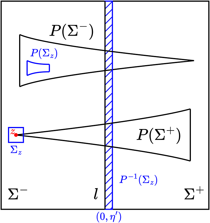
Claim 3.12. For any
 $0<\beta _0\ll 1$
, there exist
 and
 $t_0>0$
such that the cross section
 $\Sigma _z=[-1-\eta ,-1+\eta ]\times [y^+-\eta ,y^++\eta ] \subset \Sigma $
at z satisfies
-
1.
$P(\Sigma _z)\cap \Sigma _z=\emptyset $
and there exists
$\eta '>0$
such that
$P^{-1}(\Sigma _z)\subset (0,\eta ')\times [-1-\epsilon ,1+\epsilon ]$
and
$f'(x)>10$
for every (see Figure 3).Figure 3The cross section
$\Sigma _z$
in Claim 3.12. -
2. The set
and
$\phi _t^X(z)\notin \phi _{[0,3t_0]}^X(\Sigma _z)$
for each
$t<0$
. -
3. We have
$(1-\beta _0)f'(x_1)<f'(x_2)<(1+\beta _0)f'(x_1)$
for every .




 (see Figure

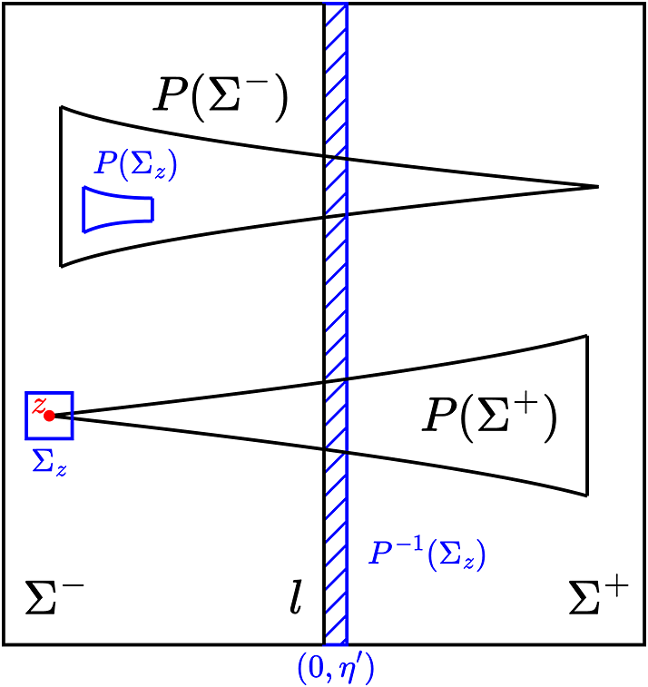
 and



 .
Proof. The fact that
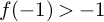 $f(-1)>-1$
implies if
 $\eta $
is small enough, then
 $f([-1-\eta ,-1+\eta ])\cap [-1-\eta ,-1+\eta ]=\emptyset $
. Thus,
 $P(\Sigma _z)\cap \Sigma _z=\emptyset $
.
Since
 $P(\Sigma )\subset [-1,1]\times (-1,1)$
, if a point
 satisfies
 , then
 . The one-dimensional map f satisfies
 $f(-1-\epsilon )>-1$
, so if
 $\eta <f(-1-\epsilon )+1$
, then there exists some
 $\eta '>0$
, such that
 $P^{-1}(\Sigma _z)\subset (0,\eta ']\times [-1-\epsilon ,1+\epsilon ]$
. If
 $\eta \rightarrow 0^+$
, then
 $\eta '\rightarrow 0^+$
, and
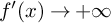 as
 . So we only need to shrink
 $\eta $
to take
 $\eta '$
small enough, such that
 $f'(x)>10$
for every
 . This shows item 1.
To verify item 2, note that
 $\Sigma _z=[-1-\eta ,-1+\eta ]\times [y^+-\eta ,y^++\eta ]$
is an
 $\eta $
-square neighborhood of
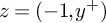 $z=(-1,y^+)$
in the cross section
 $\Sigma $
and there exists
 $t_0>0$
such that the orbit segment
 $\phi _{[-t_0,4t_0]}^X(z)\subset B(z,\delta )$
. Thus, shrinking
 $\eta $
again if necessary, the flow box
 would be contained in the open ball
 $B(z,\delta )$
. Moreover, recall that
 satisfies
 $\phi ^X_t(z)\cap \Sigma =\emptyset $
for each
 $t<0$
and
 $\Sigma _z\subset \Sigma $
; thus,
 $\phi _t^X(z)\notin \phi _{[0,3t_0]}^X(\Sigma _z)$
for each
 $t<0$
. This proves item 2.
Finally, note that
 $f'$
is continuous since the quotient map f is
 $C^1$
-smooth. Thus, by shrinking
 $\eta $
a last time if necessary, the following satisfies

As a consequence, for every  , one has
 $$\begin{align*}1-\beta_0<\frac{1}{1+\beta_0}<\frac{f'(x_2)}{f'(x_1)}<1+\beta_0,\end{align*}$$
and thus,
 $(1-\beta _0)f'(x_1)<f'(x_2)<(1+\beta _0)f'(x_1)$
which is item 3.
The subset
 $\phi _{[0,3t_0]}^X(\Sigma _z)$
admits a natural coordinate: for every
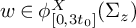 , there exist a unique point
 and
 , such that
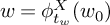 $w=\phi _{t_w}^X(w_0)$
. Then we denote

We point out here that this coordinate is only
 $C^1$
-smooth.
Let  be a smooth vector field satisfying
 $\operatorname {Supp}(Z)\subset \phi _{[t_0,2t_0]}^X(\Sigma _z)\subset B(z,\delta )$
such that if we represent Z in the coordinate
 $\{(x,y,t)\}$
as
 $$ \begin{align*} Z(x,y,t)= a(x,y,t)\cdot\frac{\partial}{\partial x}+ b(x,y,t)\cdot\frac{\partial}{\partial y}+ c(x,y,t)\cdot\frac{\partial}{\partial t}, \end{align*} $$
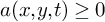
then for every  , it satisfies the following properties
-
1.
$\max \big \{ |b(x,y,t)|,|c(x,y,t)| \big \}\leq \beta |a(x,y,t)|$
and
$|a(x,y,t)|<\beta $
, where
$0<\beta <10^{-3}$
is a small constant to be determined in Claim 3.13 below. -
2.
$a(x,y,t)\geq 0$
and
$a(-1,y^+,3t_0/2)>0$
.




Here, since the coordinate
 $\{(x,y,t)\}$
is
 $C^1$
-smooth, the three functions
 $a,b,c$
are only uniformly continuous.
Claim 3.13. Let  for
 . Then there exists
 $\beta>0$
such that the
 $C^r$
-vector field family
 satisfies the following properties:
-
1.
$X_0=X$
and
$X_s$
converges to X in
$C^r$
-topology as
$s\rightarrow 0$
. -
2. For every
,
$\sigma $
is the singularity of
$X_s$
and . -
3. For every
,
$X_s|_{M^3\setminus \phi _{[t_0,2t_0]}^X(\Sigma _z)}\equiv X|_{M^3\setminus \phi _{[t_0,2t_0]}^X(\Sigma _z)}$
. -
4. For every
, the first return map
$P_s:\Sigma \setminus l\rightarrow \Sigma $
is well defined for the flow
$\phi _t^{X_s}$
and satisfies
$$ \begin{align*} P_s|_{\Sigma\setminus\Sigma_z}~\equiv~ P|_{\Sigma\setminus\Sigma_z}. \end{align*} $$
-
5. For every
, the curve
$P_s(w):[0,1]\rightarrow \Sigma $
is
$C^r$
-smooth with respect to s, and satisfies Moreover, for the point z, the curve
$P_s(z):[0,1]\rightarrow \Sigma $
satisfies
$\mathrm {d}\pi _x\circ P_s(z)/\mathrm {d}s>0$
at the point
$s=0$
.


 ,


 .
 ,

 , the first return map



 , the curve






Proof of the claim.
The definitions of Z and
 $X_s$
imply the first three items directly. The vector field X on
 $\phi _{[0,3t_0]}^X(\Sigma _z)$
is equal to
 $\partial /\partial t$
everywhere. For every w in the boundary of
 $\Sigma _z$
,
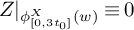 $Z|_{\phi _{[0,3t_0]}^X(w)}\equiv 0$
, this implies
 $\phi _t^{X_s}(w)=\phi _t^X(w)$
for every
 . Moreover, since

hence taking
 $0<\beta <10^{-3}$
small, for every
 and every
 , there exists some
 $t=t(w,s)$
which is close to
 $3t_0$
, such that
 . Thus, the Poincaré map from
 $\Sigma _z$
to
 $\Sigma $
associated to
 $\phi _t^{X_s}$
is well defined for every
 .
For every  , its positive orbit does not intersect
 $\phi _{[0,3t_0]}^X(\Sigma _z)$
before it enters
 $\Sigma $
again. This implies for every
 , the first return map
 $P_s:\Sigma \setminus l\rightarrow \Sigma $
is well defined for the flow
 $\phi _t^{X_s}$
and satisfies
 $P_s|_{\Sigma \setminus \Sigma _z}~\equiv ~ P|_{\Sigma \setminus \Sigma _z}$
. This proves item 4.
Let
 $$ \begin{align*} P_{s,1}:\Sigma_z\rightarrow\phi_{3t_0}^X(\Sigma_z), \qquad \mathrm{and} \qquad P_{s,2}:\phi_{3t_0}^X(\Sigma_z)\rightarrow\Sigma \end{align*} $$
be Poincaré maps of
 $\phi _t^{X_s}$
from
 $\Sigma _z$
to
 $\phi _{3t_0}^X(\Sigma _z)$
and from
 $\phi _{3t_0}^X(\Sigma _z)$
to
 $\Sigma $
, respectively. Then we have
 $P_s=P_{s,2}\circ P_{s,1}$
. Let the coordinate on
 $\phi _{3t_0}^X(\Sigma _z)$
be induced by pushing the coordinate of
 $\Sigma _z\subset \Sigma $
by
 $\phi _{3t_0}^X$
. Then
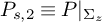 $P_{s,2}\equiv P|_{\Sigma _z}$
in this coordinate.
Since  depends continuously with respect to s in
 $\mathscr {X}^r(M^3)$
and the cross section
 $\Sigma $
is a
 $C^r$
smooth surface, the curve
 $P_s(w):[0,1]\rightarrow \Sigma $
is
 $C^r$
-smooth with respect to s for every
 .
The property
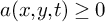 $a(x,y,t)\geq 0$
everywhere implies for every
 ,
 $\mathrm {d}\pi _x\circ P_{s,1}(w)/\mathrm {d}s\geq 0$
everywhere. Here,
 $\pi _x$
is the projection to x-coordinate on
 $\phi _{3t_0}^X(\Sigma _z)$
. Since
 $f'(x)\geq \lambda _0$
everywhere, we have
 $$ \begin{align*} \frac{\mathrm{d}\pi_x\circ P_s(w)}{\mathrm{d}s}~=~ \frac{\mathrm{d}f}{\mathrm{d}x}\cdot \frac{\mathrm{d}\pi_x\circ P_{s,1}(w)}{\mathrm{d}s} ~\geq~0. \end{align*} $$
Moreover, since
 $|b(x,y,t)|\leq \beta \cdot |a(x,y,t)|\leq 10^{-3}\cdot |a(x,y,t)|$
for every
 $(x,y,t)$
, hence for every
 and every
 $0\leq s_1<s_2\leq 1$
, we have
 $$ \begin{align*} \left|\pi_y\circ P_{s_2,1}(w)-\pi_y\circ P_{s_1,1}(w)\right| ~\leq~ 10^{-3}\cdot \left|\pi_x\circ P_{s_2,1}(w)-\pi_x\circ P_{s_1,1}(w)\right|. \end{align*} $$
This implies
 $\mathrm {d}P_{s,1}/\mathrm {d}s$
is tangent to the cone field
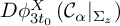 $D\phi _{3t_0}^X\left (\mathcal {C}_{\alpha }|_{\Sigma _z}\right )$
everywhere on
 $\phi _{3t_0}^X(\Sigma _z)$
. Since
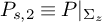 $P_{s,2}\equiv P|_{\Sigma _z}$
, and P preserves the cone field
 $\mathcal {C}_{\alpha }$
(Lemma 2.6 and Notation 3.4), the curve
 $P_s(w):[0,1]\rightarrow \Sigma $
is tangent to
 $\mathcal {C}_{\alpha }$
everywhere.
For the point  , since
 $a(-1,y^+,3t_0/2)>0$
, there exists a neighborhood of
 $(-1,y^+,3t_0/2)$
, such that for every
 $(x,y,t)$
in this neighborhood, we have
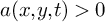 $a(x,y,t)>0$
. Thus, there exists some
 $s'>0$
and
 $\kappa>0$
, such that for every
 $0<s<s'$
, we have
 $\pi _x\circ P_{s,1}(z)\geq -1+\kappa \cdot s$
. Thus, we have
 $$ \begin{align*} \frac{\mathrm{d}\pi_x\circ P_s(z)}{\mathrm{d}s}|_{s=0}~=~ \frac{\mathrm{d}f}{\mathrm{d}x}|_{x=-1}\cdot \frac{\mathrm{d}\pi_x\circ P_{s,1}(w)}{\mathrm{d}s}|_{s=0} ~\geq~\lambda_0\cdot\kappa>0. \end{align*} $$
Then item 5 is proved, and the proof of the claim is completed.
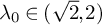
Recall in Notation 3.4 that we have fixed
 $\alpha =1/(\sqrt {2}-1)$
and there exists
 , such that
 $f'(x)>\lambda _0$
for every
 . We fix the
 -vector field Z to satisfy Claim 3.13 and a constant
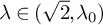 . Also, we take
 $\beta _0>0$
in Claim 3.12 small enough such that
 $$\begin{align*}\lambda(1-\beta_0(1+\alpha)(\lambda-\sqrt{2}))>\sqrt{2}.\end{align*}$$
Claim 3.14. There exists a constant  such that
 for every
 and satisfies the following two properties:
-
1. For every
, the Poincaré return map
$P_s:\Sigma \setminus l\rightarrow \Sigma $
satisfies for every ,
$$ \begin{align*} \frac{\partial\pi_x\circ P_s(x,y)}{\partial x}>\lambda, \qquad &\mathit{and} \qquad \frac{\partial\pi_x\circ P_s(x,y)}{\partial y} <\beta_0(\lambda-\sqrt{2}); \\ \left|\frac{\partial\pi_y\circ P_s(x,y)}{\partial x}\right|<1, \qquad &\mathit{and} \qquad \left|\frac{\partial\pi_y\circ P_s(x,y)}{\partial y}\right| <1. \end{align*} $$
-
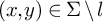
2. Let
$\gamma _0:[0,\tau ]\rightarrow \Sigma $
be defined as
$\gamma _0(s)=P_s(z)$
. Then we have
 , the Poincaré return map

 ,




Proof of the claim.
Since
 $X_s\rightarrow X$
in
 $\mathscr {X}^r(M^3)$
and
 $P_s|_{\Sigma \setminus \Sigma _z}\equiv P|_{\Sigma \setminus \Sigma _z}$
, we have
 $P_s\rightarrow P$
in
 $C^1$
-topology under the coordinate
 $\Sigma =[-1-\epsilon ,1+\epsilon ]^2$
. However,

So there exists
 $\tau _1>0$
, such that for every
 ,
 whose Poincaré map
 $P_s$
satisfies
 $\partial \pi _x\circ P_s(x,y)/\partial x>\lambda $
and
 $\partial \pi _x\circ P_s(x,y)/\partial y<\beta _0(\lambda -\sqrt {2})$
for every
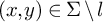 . The proof for
 $|\partial \pi _y\circ P_s(x,y)/\partial x|<1$
and
 $|\partial \pi _y\circ P_s(x,y)/\partial y|<1$
is the same.
Since
 $P_s(z)$
is
 $C^r$
-smooth with respect to
 , the function
 $\pi _x\circ P_s(z)$
is
 $C^1$
-smooth with respect to s. There exists
 $\tau _2>0$
, such that for every
 , it satisfies
 $$ \begin{align*} \frac{\mathrm{d}\pi_x\circ \gamma_0(s)}{\mathrm{d}s}|_{s=s'} ~\geq~\frac{1}{2}\cdot \frac{\mathrm{d}\pi_x\circ \gamma_0(s)}{\mathrm{d}s}|_{s=0}. \end{align*} $$
We take
 $\tau =\min \{\tau _1,\tau _2\}$
finishing the proof of the claim.
Fix  from Claim 3.14. For every
 $n\geq 1$
, let

From Item 5 of Claim 3.13 and Item 2 of Claim 3.14, both
 $\pi _x\circ \gamma _0(s)$
and
 $\pi _x\circ P_s$
are monotonous increasing with respect to the parameter s. If some
 satisfies

then there exists
 $\epsilon _s>0$
, such that

This implies
 $D_n$
is a finite subset of
 $[0,\tau ]$
and satisfies
 $D_n\subseteq D_{n+1}$
.
Claim 3.15. For every
 $n\geq 0$
, the map
 $$ \begin{align*} \gamma_n(s)=\left(x_n(s),~y_n(x)\right)=P_s^n\circ\gamma_0(s): ~[0,\tau]\setminus D_n\longrightarrow\Sigma \end{align*} $$
is well defined. For each connected component J of
 $[0,\tau ]\setminus D_n$
,
 $\gamma _n$
is a diffeomorphism from J to its image and satisfies

Proof of the claim.
We prove this claim by induction. When
 $n=0$
, the item 5 of Claim 3.13 shows that
 for every
 . And
 $x_0'(s)\geq \lambda ^0 x_0'(s)$
automatically holds for every
 . Now we assume for every
 $0\leq i\leq n-1$
and every
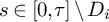 ,

For every  , we have
 $$ \begin{align*} x_n(s)=\pi_x\circ P_s\left(x_{n-1}(s),y_{n-1}(s)\right), \qquad \mathrm{and} \qquad y_n(s)=\pi_y\circ P_s\left(x_{n-1}(s),y_{n-1}(s)\right). \end{align*} $$
Now we fix  . There are two possibilities: either
 $(x_{n-1}(s_0),y_{n-1}(s_0))\notin \Sigma _z$
or
 . If
 $(x_{n-1}(s_0),y_{n-1}(s_0))\notin \Sigma _z$
, then there exists a neighborhood of
 $(x_{n-1}(s_0),y_{n-1}(s_0))$
, such that
 $P_s\equiv P$
in this neighborhood. Lemma 2.6 shows that

If  , item 1 of Claim 3.12 implies
 $(x_{n-2}(s_0),y_{n-2}(s_0))\notin \Sigma _z$
,
 $0<x_{n-2}(s_0)<\eta '$
and
 $f'(x_{n-2}(s_0))>10$
. If we denote

then
 $\gamma _{n-1}'(s_0)= \left (DP|_{(x_{n-2}(s_0),y_{n-2}(s_0))}\right ) \big (\gamma _{n-2}'(s_0)\big )$
. Thus, we have
 $$ \begin{align*} \left|y_{n-2}'(s_0)\right|\leq \alpha\cdot\left|x_{n-2}'(s_0)\right|, \qquad |x_{n-1}'(s_0)|=f'(x_{n-2}(s_0))\cdot|x_{n-2}'(s_0)| \geq 10|x_{n-2}'(s_0)|, \end{align*} $$
and
 $$ \begin{align*} |y_{n-1}'(s_0)|~&\leq~ \frac{\partial H}{\partial x}|_{\gamma_{n-2}(s_0)} \cdot|x_{n-2}'(s_0)|~+~ \frac{\partial H}{\partial y}|_{\gamma_{n-2}(s_0)} \cdot|y_{n-2}'(s_0)| \\ &\leq~ |x_{n-2}'(s_0)|~+~|y_{n-2}'(s_0)| \\ &\leq~(1+\alpha)|x_{n-2}'(s_0)|. \end{align*} $$
Now we calculate
 $\gamma _n'(s_0)$
. Since
 $x_n(s)=\pi _x\circ P_s\left (x_{n-1}(s),y_{n-1}(s)\right )$
and
 $y_n(s)=\pi _y\circ P_s\left (x_{n-1}(s),y_{n-1}(s)\right )$
, if we denote
 $w_{n-1}=\left (x_{n-1}(s_0),y_{n-1}(s_0)\right )$
, then
 $$ \begin{align*} x_n'(s_0)= \frac{\partial \pi_x\circ P_{s_0}}{\partial x} \cdot x_{n-1}'(s_0) + \frac{\partial \pi_x\circ P_{s_0}}{\partial y} \cdot y_{n-1}'(s_0) + \frac{\partial \pi_x\circ P_s(w_{n-1})}{\partial s} |_{s=s_0}. \end{align*} $$
From item 1 of Claim 3.14, we have
 $$ \begin{align*} \frac{\partial \pi_x\circ P_{s_0}}{\partial x} \cdot x_{n-1}'(s_0) \geq \lambda\cdot x_{n-1}'(s_0) \quad \mathrm{and} \quad \left|\frac{\partial \pi_x\circ P_{s_0}}{\partial y} \cdot y_{n-1}'(s_0)\right| \leq \beta_0(\lambda-\sqrt{2})\cdot|y_{n-1}'(s_0)|. \end{align*} $$
Since
 $|y_{n-1}'(s_0)|\leq \alpha \cdot x_{n-1}'(s_0)$
and
 $\lambda (1-\beta _0(1+\alpha )(\lambda -\sqrt {2}))>\sqrt {2}$
, we have
 $$ \begin{align} x_n'(s_0)\geq \sqrt{2}\cdot x_{n-1}'(s_0) + \frac{\partial \pi_x\circ P_s(w_{n-1})}{\partial s} |_{s=s_0}. \end{align} $$
However, we have
 $$ \begin{align*} y_n'(s_0)=\frac{\partial \pi_y\circ P_{s_0}}{\partial x} \cdot x_{n-1}'(s_0) + \frac{\partial \pi_y\circ P_{s_0}}{\partial y} \cdot y_{n-1}'(s_0) + \frac{\partial \pi_y\circ P_s(w_{n-1})}{\partial s} |_{s=s_0}. \end{align*} $$
Again, item 1 of Claim 3.14 shows that
 $|\partial \pi _y\circ P_{s_0}/\partial x|<1$
and
 $|\partial \pi _y\circ P_{s_0}/\partial y|<1$
. Thus, we have
 $$ \begin{align} |y_n'(s)|<(1+\alpha)\cdot x_{n-1}'(s_0)+ \left|\frac{\partial \pi_y\circ P_s(w_{n-1})}{\partial s} |_{s=s_0}\right|. \end{align} $$
Item 5 of Claim 3.13 shows that

which implies
 $$ \begin{align} \left|\frac{\partial \pi_y\circ P_s(w_{n-1})}{\partial s}|_{s=s_0}\right| ~\leq~\alpha\cdot \frac{\partial \pi_x\circ P_s(w_{n-1})}{\partial s}|_{s=s_0}. \end{align} $$
Since
 $\alpha =1/(\sqrt {2}-1)$
which is equivalent to
 $(1+\alpha )/\sqrt {2}=\alpha $
, Equation 3.1 and Equation 3.2 imply

Finally, Equation 3.1 and Equation 3.3 show that
 $$ \begin{align*} x_n'(s_0)~\geq~\sqrt{2}\cdot x_{n-1}'(s_0) ~\geq~ 10\sqrt{2}\cdot x_{n-2}'(s_0) ~>~ \lambda^2\cdot\lambda^{n-2} ~=~ \lambda^n. \end{align*} $$
This finishes the proof of the claim.
We can finish the proof of this theorem by using the idea of Lemma 3.6.
Claim 3.16. There exists some integer
 $N>0$
, such that
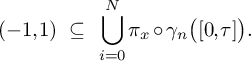 $$ \begin{align*} (-1,1)~\subseteq~ \bigcup_{i=0}^N\pi_x\circ\gamma_n\big([0,\tau]\big). \end{align*} $$
Proof of the claim.
If
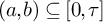 $(a,b)\subseteq [0,\tau ]$
is a connected component of
 $[0,\tau ]\setminus D_n$
, then
 $$ \begin{align*} \pi_x\circ\gamma_n(s)=\pi_x\circ P_s^n\circ\gamma_0(s): ~[0,\tau]\rightarrow[-1,1] \end{align*} $$
is a diffeomorphism from
 $(a,b)$
to its image.
Similar to Claim 3.7, we show that for every
 $n\geq 1$
, let
 $I=(a,b)$
be a connected component of
 $[0,\tau ]\setminus D_n$
. Then either
 $\#\big (I\cap D_{n+2}\big )\leq 1$
or
 $(-1,1)\subseteq \pi _x\circ \gamma _{n+1}(I)\cup \pi _x\circ \gamma _{n+2}(I)$
.
Actually, let
 $(c,d)=\pi _x\circ \gamma _n(I)$
. If
 $0\notin (c,d)$
, then
 $I\cap D_{n+1}=\emptyset $
and
 $$ \begin{align*} \pi_x\circ\gamma_{n+1}(I)= \pi_x\circ P_s^{n+1}\circ\gamma_0(I) \end{align*} $$
is an open interval in
 $(-1,1)$
. Thus, there exists at most one point
 satisfying
 $\pi _x\circ \gamma _{n+1}(s_0)=0$
. This implies
 $\#\big (I\cap D_{n+2}\big )\leq 1$
.
If  , then we denote
 satisfying
 $\pi _x\circ \gamma _n(s_0)=\pi _x\circ P_{s_0}^n\circ \gamma _0(s_0)=0$
. Then two open intervals
 $(a,s_0)$
and
 $(s_0,b)$
are two connected components of
 $I\setminus D_{n+1}$
. Moreover, item 4 of Claim 3.13 shows that
 $P_s|_{\Sigma \setminus \Sigma _z}\equiv P|_{\Sigma \setminus \Sigma _z}$
. This implies
 $$ \begin{align*} \lim_{s\rightarrow s_0^-}\pi_x\circ\gamma_{n+1}(s)=1, \qquad \mathrm{and} \qquad \lim_{s\rightarrow s_0^+}\pi_x\circ\gamma_{n+1}(s)=-1. \end{align*} $$
Thus, there exists  , such that
 $$ \begin{align*} \pi_x\circ\gamma_{n+1}\big( (a,s_0) \big)=(e_1,1), \qquad \mathrm{and} \qquad \pi_x\circ\gamma_{n+1}\big( (s_0,b) \big)=(-1,e_2). \end{align*} $$
If both of them do not contain
 $0$
, then we have
 $\#\big (I\cap D_{n+2}\big )=\#\big (I\cap D_{n+1}\big )=1$
.
Otherwise, we have either  or
 . Thus, either
 $$ \begin{align*} [0,1)\subset \pi_x\circ\gamma_{n+1}\big( (a,s_0) \big) \subset \pi_x\circ\gamma_{n+1}(I), \qquad \mathrm{or} \qquad (-1,0]\subset \pi_x\circ\gamma_{n+1}\big( (s_0,b) \big) \subset \pi_x\circ\gamma_{n+1}(I). \end{align*} $$
In both cases, we can apply
 $P_s|_{\Sigma \setminus \Sigma _z}\equiv P|_{\Sigma \setminus \Sigma _z}$
and show that
 $$ \begin{align*} (-1,1)\subseteq \pi_x\circ\gamma_{n+1}(I)\cup \pi_x\circ\gamma_{n+2}(I). \end{align*} $$
Now we claim there exists some
 $n>0$
and a connected component I of
 $[0,\tau ]\setminus D_n$
, such that
 $(-1,1)\subseteq \pi _x\circ \gamma _{n+1}(I)\cup \pi _x\circ \gamma _{n+2}(I)$
. Otherwise, we have
 $$ \begin{align*} \# D_2\leq1, \qquad \# D_4\leq\# D_2+\# D_2+1\leq 3, \qquad \cdots \qquad \# D_{2n}\leq \# D_{2n-2}+\# D_{2n-2}+1\leq 2^n-1. \end{align*} $$
This implies
 $[0,\tau ]\setminus D_{2n}$
has at most
 $2^n$
connected components. So there exists a connected component
 $I_{2n}\subset [0,\tau ]\setminus D_{2n}$
, such that its length satisfies
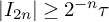 $|I_{2n}|\geq 2^{-n}\tau $
.
Since
 $\pi _x\circ \gamma _{2n}$
is a diffeomorphism on each connected component of
 $[0,\tau ]\setminus D_{2n}$
, and Claim 3.15 shows that

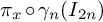
the length of the interval
 $\pi _x\circ \gamma _n(I_{2n})$
satisfies
 $|\pi _x\circ \gamma _n(I_{2n})| \geq \lambda ^{2n}\cdot |\gamma _0(I_{2n})|$
.
Finally, item 2 of Claim 3.14 shows that
 $$ \begin{align*} |\gamma_0(I_{2n})|~\geq~\frac{1}{2}\cdot \frac{\mathrm{d}\pi_x\circ \gamma_0(s)}{\mathrm{d}s}|_{s=0} \cdot|I_{2n}| ~\geq\frac{1}{2}\cdot \frac{\mathrm{d}\pi_x\circ \gamma_0(s)}{\mathrm{d}s}|_{s=0}\cdot 2^{-n}\tau. \end{align*} $$
Thus, we have

This is absurd because
 $\pi _x\circ \gamma _n(I_{2n})\subseteq (-1,1)$
. So there exists
 $n>0$
and a connected component I of
 $[0,\tau ]\setminus D_n$
, such that
 $(-1,1)\subseteq \pi _x\circ \gamma _{n+1}(I)\cup \pi _x\circ \gamma _{n+2}(I)$
. We take
 $N=n+2$
to complete the proof of this claim.
For the critical point  , recall that
 $l_p=\{x_p\}\times [-1-\epsilon ,1+\epsilon ]\subset \Sigma $
with
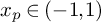 (if
 $p=\sigma $
, then
 $x_p=0$
). Claim 3.16 shows there exist
 and
 $n>0$
, such that
 $$ \begin{align*} x_p~=~\pi_x\circ P_s^n\circ\gamma_0(s) ~=~\pi_x\circ P_s^n\circ P_s(z). \end{align*} $$
This implies for the vector field  , there exists
 $T>0$
, such that
 .
Since
 $X_s|_{M^3\setminus B(z,\delta )}\equiv X|_{M^3\setminus B(z,\delta )}$
and
 $B(z,\delta )\cap \left (\bigcup _{t\geq 0}\phi _t^X(l_p)\cup \{\sigma \}\right ) =\emptyset $
, we have
 $l_p\subset W^s_{\mathit {loc}}(\operatorname {Orb}(p),\phi _t^Y)$
. The fact
 implies
 $$ \begin{align*} \operatorname{Orb}(z,\phi_t^Y)~\subset~ W^u(\sigma,\phi_t^Y) \cap W^s(\operatorname{Orb}(p),\phi_t^Y). \end{align*} $$
This completes the proof of this theorem.
4 The space of ergodic measures for Lorenz attractors
In this section, we aim to prove Theorem B and Corollary 1.4. We would also obtain properties concerning path connectedness and denseness of periodic measures for ergodic measure space for more general invariant sets.
4.1 Path connectedness
This subsection devotes to give a general criterion for path connectedness (or arcwise connectedness) of the ergodic measure space. More precisely, for a homoclinic class
 $\Lambda $
of a vector field
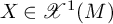 , if all periodic orbits are homoclinically related with each other, then the set of ergodic measures supported on
 $\Lambda $
which can be approximated by periodic measures is path connected. A related conclusion for diffeomorphisms is proved in [Reference Gorodetski and Pesin31].
Proposition 4.1. Let 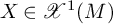 and
 $\Lambda $
be a homoclinic class of X such that all periodic points in
 $\Lambda $
are hyperbolic and any two periodic points in
 $\Lambda $
are homoclinically related. Then the set
 $\overline {\mathcal {M}_{per}(\Lambda )}\cap \mathcal {M}_{erg}(\Lambda )$
is path connected.
The proof of Proposition 4.1 follows the idea of [Reference Gorodetski and Pesin31, Theorem 1.1, 1.2]. We first prove the following two lemmas which are the version of [Reference Gorodetski and Pesin31, Lemma 3.1, 3.2] for vector fields. Given a periodic point p, we denote by
 $\delta _{\operatorname {Orb}(p)}$
the periodic measures corresponding to
 $\operatorname {Orb}(p)$
. The first lemma states that any two periodic measures can be connected through a path inside
 $\overline {\mathcal {M}_{per}(\Lambda )}\cap \mathcal {M}_{erg}(\Lambda )$
.
Lemma 4.2. Under hypothesis of Proposition 4.1, for any two periodic points  , there exists a continuous path
 such that
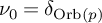 $\nu _0=\delta _{\operatorname {Orb}(p)}$
and
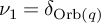 $\nu _1=\delta _{\operatorname {Orb}(q)}$
.
Proof. Since the two hyperbolic periodic orbits
 $\operatorname {Orb}(p)$
and
 $\operatorname {Orb}(q)$
are homoclinically related, there exists a hyperbolic horseshoe
 $K\subset \Lambda $
of X containing p and q. Note here that the hypberolic horseshoe K of X is the suspension of a hyperbolic horseshoe
 $\tilde {K}$
for a diffeomorphism (the time one map of the flow) with a continuous roof function. By [Reference Sigmund66, Theorem B], the space
 $\mathcal {M}_{erg}(\tilde {K})$
is path connected. However, there is a one-to-one correspondence between
 $\mathcal {M}_{erg}(\tilde {K})$
and
 $\mathcal {M}_{erg}(K)$
; see, for, instance [Reference Parry and Pollicott54, Chapter 6]. Hence,
 $\mathcal {M}_{erg}(K)$
is path connected. Moreover,
 $\mathcal {M}_{per}(K)$
is dense in
 $\mathcal {M}_{erg}(K)$
since K is a hyperbolic horseshoe. Thus,
 $\delta _{\operatorname {Orb}(p)}$
and
 $\delta _{\operatorname {Orb}(q)}$
can be connected by a path contained in
 $\mathcal {M}_{erg}(K)\subset \overline {\mathcal {M}_{per}(\Lambda )}\cap \mathcal {M}_{erg}(\Lambda )$
.
The next lemma states that if two periodic measures are both close to a same ergodic measure
 $\mu $
, then there is a short path in the ergodic measure space connecting them in the sense that the whole path is close to
 $\mu $
.
Lemma 4.3. Under hypothesis of Proposition 4.1, for any  and
 $\varepsilon>0$
, there exists
 $\eta>0$
such that if two periodic points
 satisfy
 $d(\mu ,\delta _{\operatorname {Orb}(p)})<\eta $
and
 $d(\mu ,\delta _{\operatorname {Orb}(q)})<\eta $
, then there exists a path
 such that
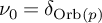 $\nu _0=\delta _{\operatorname {Orb}(p)}$
,
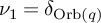 $\nu _1=\delta _{\operatorname {Orb}(q)}$
and
 $d(\mu ,\nu _t)<\varepsilon $
for any
 .
Proof. Since
 $\operatorname {Orb}(p)$
and
 $\operatorname {Orb}(q)$
are homoclinically related, there exist hyperbolic horseshoes such that every point in which spends arbitrarily large fractions of its orbit shadowing
 $\operatorname {Orb}(p)$
and
 $\operatorname {Orb}(q)$
as closely as we want. Thus, we can choose a hyperbolic horseshoe K containing p and q such that any ergodic measure supported on K is
 $\eta $
-close to
 $\delta _{\operatorname {Orb}(p)}$
or
 $\delta _{\operatorname {Orb}(q)}$
. As a consequence, the horseshoe K is
 $2\eta $
-close to
 $\mu $
in the measure sense: any ergodic measure supported on K is contained in the
 $2\eta $
-neighborhood of
 $\mu $
. By [Reference Sigmund66, Theorem B], there is a continuous path
 connecting
 $\delta _{\operatorname {Orb}(p)}$
and
 $\delta _{\operatorname {Orb}(q)}$
, satisfying
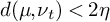 $d(\mu ,\nu _t)<2\eta $
for any
 . Then Lemma 4.3 concludes if we take
 $\eta =\varepsilon /2$
.
Now we could complete the proof of Proposition 4.1.
Proof of Proposition 4.1.
Take two ergodic measures  . We only need to show there exists a path
 such that
 $\mu _0=\mu $
and
 $\mu _1=\nu $
. We follow the idea of [Reference Gorodetski and Pesin31, Theorem 1.1]. By assumption, there exist two sequences of periodic points
 $\{p_n\}$
and
 $\{q_n\}$
in
 $\Lambda $
such that
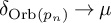 $\delta _{\operatorname {Orb}(p_n)}\rightarrow \mu $
and
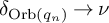 $\delta _{\operatorname {Orb}(q_n)}\rightarrow \nu $
in the weak*-topology. Taking subsequences if necessary, we assume
 $$\begin{align*}d(\delta_{\operatorname{Orb}(p_n)},\mu)<\frac{1}{2\cdot3^n} \text{~~and~~} d(\delta_{\operatorname{Orb}(q_n)},\nu)<\frac{1}{2\cdot3^n}, \text{ for all }n\geq 1. \end{align*}$$
By Lemma 4.2, there exists a continuous path  such that
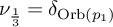 $\nu _{\frac {1}{3}}=\delta _{\operatorname {Orb}(p_1)}$
and
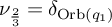 $\nu _{\frac {2}{3}}=\delta _{\operatorname {Orb}(q_1)}$
. By Lemma 4.3, for any
 $n\geq 1$
, there exist two paths

in
 $\overline {\mathcal {M}_{per}(\Lambda )}\cap \mathcal {M}_{erg}(\Lambda )$
connecting
 $\delta _{\operatorname {Orb}(p_n)},\delta _{\operatorname {Orb}(p_{n+1})}$
and
 $\delta _{\operatorname {Orb}(q_n)},\delta _{\operatorname {Orb}(q_{n+1})}$
, respectively, and the length of the paths decreases to 0 exponentially when n goes to
 . Therefore,
 is a continuous path in
 $\overline {\mathcal {M}_{per}(\Lambda )}\cap \mathcal {M}_{erg}(\Lambda )$
satisfying that
 $\nu _0=\mu $
and
 $\nu _1=\nu $
. This completes the proof.
4.2 Homoclinic loop and periodic measures
In this subsection, we prove that a homoclinic loop of a singularity can be accumulated by periodic orbits with the associated periodic measures accumulating to the singular measure by
 $C^r$
-perturbations.
Proposition 4.4. Let 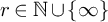 and
 be a
 $C^r$
-vector field on M. If
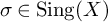 is a hyperbolic singularity of X, and
 $$ \begin{align*} \Gamma=\operatorname{Orb}(z,\phi_t^X)\subset W^s(\sigma,\phi_t^X)\cap W^u(\sigma,\phi_t^X) \end{align*} $$
is a homoclinic orbit of
 $\sigma $
, then there exist a sequence of vector fields
 $\{X_n\}$
and a sequence of periodic points
 , such that
-
1. The vector field
$X_n$
converges to X in
$\mathscr {X}^r(M)$
. -
2.
and the periodic measure
$\delta _{\operatorname {Orb}(p_n,\phi _t^{X_n})}$
converges to
$\delta _{\sigma }$
. -
3. The orbit
$\operatorname {Orb}(p_n,\phi _t^{X_n})$
converges to
$\Gamma \cup \{\sigma \}$
in the Hausdorff topology.


 and the periodic measure
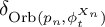

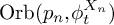

Proof. Let
 $d=\dim M$
and
 $s=\dim E^s(\sigma )$
be the index of
 $\sigma $
. Then
 $\dim E^u(\sigma )=d-s$
. Since
 $\Gamma =\operatorname {Orb}(z,\phi _t^X)$
is a homoclinic loop of X, we have
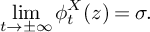
By Grobman-Hartman Theorem [Reference de Melo and Palis27, 4.10 Theorem], there exists a small neighborhood
 $U(\sigma )$
of
 $\sigma $
, such that the flow
 $\phi _t^X$
is orbit equivalent to the linear system generated by
 $DX(\sigma )$
. Moreover, shrinking
 $U(\sigma )$
if necessary, we can assume there exist
 $T_1<0<T_2$
satisfying

where  and
 .
There exists a
 $(d-1)$
-dimensional
 -smooth cross section
 $\Sigma _1$
which is transverse to X everywhere and satisfies the following properties:
-
•
, and
$\phi _{[0,1]}^X(\Sigma _1)\cap \Gamma =\phi _{[T_1-1,T_1]}^X(z)$
. -
• There exists a s-dimensional
-smooth disk
$\Sigma _1^s\subset \Sigma _1$
such that
$\Sigma _1^s$
is transverse to
$W^u_{\mathit {loc}}(\sigma )$
at
$\phi _{T_1-1}^X(z)$
.
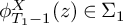 , and

 -smooth disk


Symmetrically, there exists a
 $(d-1)$
-dimensional
 -smooth cross section
 $\Sigma _2$
which is transverse to X everywhere and satisfies the following properties:
-
•
, and
$\phi _{[-1,0]}^X(\Sigma _2)\cap \Gamma =\phi _{[T_2,T_2+1]}^X(z)$
; -
• there exists a
$(d-s)$
-dimensional -smooth disk
$\Sigma _2^u\subset \Sigma _2$
such that
$\Sigma _2^u$
is transverse to
$W^s_{\mathit {loc}}(\sigma )$
at
$\phi _{T_2+1}^X(z)$
.
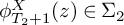 , and


 -smooth disk


By the
 $\lambda $
-lemma (Inclination Lemma) (see [Reference de Melo and Palis27, 7.2 Lemma]), there exists a sequence of points
 and
 , such that
-
1. The point
$x_n\rightarrow \phi _{T_2+1}^X(z)$
in
$\Sigma _2^u$
as . -
2. The point
, and
$y_n\rightarrow \phi _{T_1-1}^X(z)$
in
$\Sigma _1^s$
as . -
3. The orbit segment
$\phi _{[0,S_n]}^X(x_n)\subset U(\sigma )$
for every n.


 .
 , and


 .

Now we consider two flow boxes
 $V_1=\phi _{[T_1-1,T_1]}^X(\Sigma _1)$
and
 $V_2=\phi _{[T_2,T_2+1]}^X(\Sigma _2)$
. Since
 $x_n\rightarrow \phi _{T_2+1}^X(z)$
in
 $\Sigma _2^u$
and
 $y_n\rightarrow \phi _{T_1-1}^X(z)$
in
 $\Sigma _1^s$
, there exists a sequence of vector fields
 , such that
-
1. The vector field
$X_n$
converges to X in
$C^r$
-topology. -
2.
$X_n|_{M\setminus (V_1\cup V_2)}\equiv X|_{M\setminus (V_1\cup V_2)}$
. -
3. There exist
$a_n,b_n\rightarrow 1$
as , such that
$$ \begin{align*} \phi_{a_n}^{X_n}(y_n)=\phi_{T_1}^X(z), \qquad \mathrm{and} \qquad \phi_{b^n}^{X_n}\big( \phi_{T_2}^X(z) \big)=x_n. \end{align*} $$




 , such that

This implies the vector field
 $X_n$
satisfies
 $\phi _{b_n+S_n+a_n}^{X_n}\big (\phi _{T_2}^X(z)\big )=\phi _{T_1}^X(z)$
. So
 $\Gamma _n=\operatorname {Orb}(z,\phi _t^{X_n})$
is a periodic orbit of
 $X_n$
with period
 $\pi _n=a_n+b_n+(T_2-T_1)+S_n$
. Moreover, we have

Recall that  and
 $y_n\rightarrow \phi _{T_1-1}^X(z)$
. Since
 $(\pi _n-S_n)$
is uniformly bounded above, the fact that
 $$ \begin{align*} \phi_{[0,S_n]}^{X_n}(x_n)=\phi_{[0,S_n]}^X(x_n)\subseteq U(\sigma) \end{align*} $$
and
 $\phi _t^X$
is orbit equivalent to the linear system generated by
 $DX(\sigma )$
in
 $U(\sigma )$
implies
 $\Gamma _n$
converges to
 $\Gamma \cup \{\sigma \}$
in the Hausdorff topology and the periodic measure
 $\delta _{\Gamma _n}$
converges to
 $\delta _{\sigma }$
.
4.3 Isolated singular measures: a criterion
In this subsection, we show that if the unstable manifold of a codimension one singularity is contained in the stable manifold of a periodic orbit, then the Dirac measure of this singularity is isolated in the space of ergodic measures. The idea of this proposition is inspired by the work of J. Palis [Reference Palis55]; see also [Reference de Melo and Palis26].
Proposition 4.5. Let 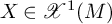 and
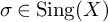 be a hyperbolic singularity satisfying
 $\dim E^u(\sigma )=1$
. Assume there exists a hyperbolic periodic point
 such that
 $W^u(\sigma )\setminus \{\sigma \}\subset W^s(\operatorname {Orb}(p))$
. Then the Dirac measure
 $\delta _{\sigma }$
is isolated in
 $\mathcal {M}_{erg}(X)$
.
Remark 4.6. Note that
 $\dim E^u(\sigma )=1$
implies
 $W^u(\sigma )$
consists two branches, each of which is a single orbit. Proposition 4.5 gives a general criterion to obtain isolated ergodic measures inside a (nontrivial) transitive set. For instance, when the hyperbolic singularity
 $\sigma $
of X is contained in a homoclinic class
 $\Lambda $
and if one could make
 $W^u(\sigma )\setminus \{\sigma \}\subset W^s(\operatorname {Orb}(p))$
through
 $C^r (r\geq 1)$
perturbations where
 $\operatorname {Orb}(p)$
is a hyperbolic periodic orbit, then
 $\delta _\sigma $
is isolated in
 $\mathcal {M}_{erg}(Y)$
, where Y is the resulting vector field after perturbation. See the dense part of Theorem B.1 in Appendix B.
Proof. Assume there exists a sequence of ergodic measures
 $\mu _n$
approximating the Dirac measure
 $\delta _{\sigma }$
. We only need to find a continuous function
 $\varphi :M\rightarrow {\mathbb R}$
, such that
 does not converge to
 . Then we get a contradiction.
Since
 $\sigma $
is a hyperbolic singularity, each
 $\mu _n$
does not support on a singularity. Let
 be a generic point of
 $\mu _n$
(i.e., the empirical measure equidistributed on the orbit segment
 $\phi _{[0,T]}(x_n)$
converges to
 $\mu _n$
as
 ). We must have
 $\operatorname {Ind}(p)<d-1$
. Otherwise,
 $\operatorname {Orb}(p)$
is a periodic sink. Hence, as the positive orbit of
 $x_n$
approaches
 $\sigma $
, it also approaches
 $W^u(\sigma )$
and enters the attracting region of
 $\operatorname {Orb}(p)$
. This contradicts
 , which implies that
 $x_n$
is a recurrent point.
As we have assumed
 $\dim E^u(\sigma )=1$
, let
 $\lambda _1,\cdots ,\lambda _d$
be eigenvalues of
 $DX(\sigma )$
which satisfy
 $|\mathrm {Re}\lambda _1 |\leq \cdots \leq |\mathrm {Re}\lambda _{d-1}| < 1< |\mathrm {Re}\lambda _d|=|\lambda _d |$
. We fix a constant
 $\epsilon _1$
satisfying
 $0<\epsilon _1<\min \big \{-\log |\mathrm {Re}\lambda _{d-1}|,\log |\lambda _d|\big \}$
, and let
 $$ \begin{align} u_1=\log|\mathrm{Re}\lambda_{d-1}|+\epsilon_1<0. \end{align} $$
Claim 4.7. There exists a neighborhood
 $U(\sigma )$
of
 $\sigma $
admitting a
 $C^1$
-coordinate

such that
-
1. The singularity
, and the local stable and unstable manifolds of
$\sigma $
in
$U(\sigma )$
are
$$ \begin{align*} W^s_{\mathit{loc}}(\sigma)=\big\{(x,0):~\|x\|\leq1\big\}, \qquad \mathit{and} \qquad W^u_{\mathit{loc}}(\sigma)=\big\{(0,y):~|y|\leq1\big\}. \end{align*} $$
-
2. For every
, let
$\phi _t(z)=\big (x(t),y(t)\big )$
be the orbit of z under
$\phi _t$
where
$\big (x(0),y(0)\big )=(x,y)$
. Assume the orbit segment
$\phi _{[T_1,T_2]}(z)\subset U(\sigma )$
, where
$T_1<0<T_2$
. Then it satisfies
$|y'(t)-\lambda _d\cdot y(t)|\leq \epsilon _1\cdot |y(t)|,~~\forall T_1\leq t \leq T_2$
,
$$ \begin{align*} \|x(t)\|\leq\exp(u_1 t)\|x(0)\|, ~~\forall 0\leq t \leq T_2; \quad\!\! \mathit{and}\!\! \quad \|x(t)\|\geq\exp(u_1 t)\|x(0)\|, ~~\forall T_1\leq t\leq0. \end{align*} $$
-
3.
$U(\sigma )\cap \operatorname {Orb}(p,\phi _t)=\emptyset $
, and for , they satisfy
$\phi _t(z^\pm )\notin U(\sigma )$
for every
$t>0$
.
 , and the local stable and unstable manifolds of



 , let








 , they satisfy


Proof of Claim 4.7.
The first two items have been proved in Lemma 2.1, Theorem 2.4 and Theorem 2.5 of [Reference Shilnikov, Shilnikov, Turaev and Chua63]. The third item comes from the fact that 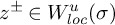 while their orbits
 $\operatorname {Orb}(z^\pm )\subseteq W^s(\operatorname {Orb}(p))$
. So we only need to take
 $U(\sigma )$
small enough.
For every
 $0<\delta <1$
, we denote
 . Let

Then
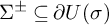 $\Sigma ^{\pm }\subseteq \partial U(\sigma )$
. Moreover, the second item of Claim 4.7 shows that the vector field X is transverse to
 $\Sigma ^{\pm }$
and points outside
 $U(\sigma )$
. For every
 $\delta>0$
,
 $\Sigma ^\pm $
are local cross sections of X centered at
 $z^\pm $
, respectively.
Claim 4.8. For every
 $0<\delta <1$
and
 with
 $x_z\neq 0,y_z>0$
, it satisfies
-
1. There exist
$T_1<0<T_2$
such that , , and for every . -
2. There exist
and , such that
$\phi _{[T_1,T_2]}(z)\cap U(\sigma ,\delta )=\phi _{[T_1',T_2']}(z)$
. -
3. If
, then we have
$\|x_w\|<\delta <1$
and
$$ \begin{align*} T_2'-T_1'~\leq~T_2-T_1~\leq~ \frac{1}{u_1}\cdot\big[\log\|x_w\|-\log1\big] ~=~\frac{1}{u_1}\cdot\log\|x_w\|. \end{align*} $$

 ,
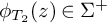 , and
 for every
 .
 and
 , such that

 , then we have


The same conclusion holds for
 $x_z\neq 0,y_z<0$
if we replace
 $\Sigma ^+$
by
 $\Sigma ^-$
.
Proof of Claim 4.8.
From the second item of Claim 4.7, for
 $z=(x,y)$
satisfying
 $x\neq 0$
and
 $y>0$
, the flow
 $\big (x(t),y(t)\big )$
satisfies
-
•
$y(t)>0$
and monotonous increasing with respect to t, which implies
$\exists T_2>0$
such that ; -
•
$\|x(t)\|\geq \exp (u_1 t)\|x(0)\|$
for every
$t\leq 0$
, which implies
$\exists T_1<0$
, such that .


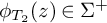 ;



 .
Moreover, we have  for every
 . This proves the first item. The proof of second item is the same.
As
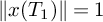 $\|x(T_1)\|=1$
and
 $\|x(T_2)\|=\|x_w\|\leq \exp (u_1 T_2)\|x\|<\delta $
, we apply the fact that
 $\|x(t)\|\geq \exp (u_1 t)\|x(0)\|$
for every
 $t\leq 0$
, which shows
 $$ \begin{align*} T_2'-T_1'~\leq~T_2-T_1~\leq~ \frac{1}{u_1}\cdot\big(\log\|x_w\|-\log1\big) ~=~\frac{1}{u_1}\cdot\log\|x_w\|.\\[-34pt] \end{align*} $$
Recall p is a hyperbolic periodic point of X with index
 $0<\operatorname {Ind}(p)<d-1$
. We denote
 $k=\operatorname {Ind}(p)$
. Then we have the following claim.
Claim 4.9. There exist a cross section
 $\Sigma _p$
transverse to X everywhere admitting a
 $C^1$
coordinate

and two constants
 $\kappa>1,~T_0>0$
, such that
-
1. The orbit
$\operatorname {Orb}(p,\phi _t)\cap \Sigma _p=\{p\}$
and . -
2. The local stable and unstable manifolds of the orbit of p intersect
$\Sigma _p$
as
$$ \begin{align*} W^s_{\mathit{loc}}(\operatorname{Orb}(p))\cap\Sigma_p= \big\{ (r,0):\|r\|\leq1 \big\}, \qquad W^u_{\mathit{loc}}(\operatorname{Orb}(p))\cap\Sigma_p= \big\{ (0,s):\|s\|\leq1 \big\}. \end{align*} $$
-
3. The Poincaré return map
is well defined and
$C^1$
-smooth on
$\Sigma _p'$
. For every , if we denote
$(r_1,s_1)=R(r,s)$
, then
$$ \begin{align*} \|r_1\|<\|r_0\|, \qquad \mathrm{and} \qquad \|s_1\|\leq\kappa\cdot\|s_0\|. \end{align*} $$
-
4. For every
, let
$T_z>0$
be the first return time of z to
$\Sigma _p$
(i.e. ). Then
$T_z\geq T_0$
and

 .





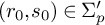 , if we denote


 , let


 ). Then

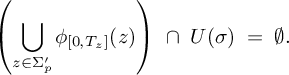
Proof of Claim 4.9.
Let
 $\pi (p)$
be the period of p and
 $u_2>0$
be the largest Lyapunov exponent of
 $\operatorname {Orb}(p)$
. There exists a
 $C^1$
cross section
 $\Sigma _1$
containing p and transversing to X everywhere. By shrinking
 $\Sigma _1$
if necessary, we can assume
 $\Sigma _1\cap \operatorname {Orb}(p,\phi _t)=\{p\}$
.
Since p is a hyperbolic periodic orbit of X, there exists a small neighborhood
 $\Sigma _2\subseteq \Sigma _1$
, such that the Poincaré map
 $R:\Sigma _2\rightarrow \Sigma _1$
is well defined and
 $C^1$
-smooth. Moreover, p is a hyperbolic fixed point of R with largest Lyapunov exponent equal to
 $\big (\pi (p)u_2\big )$
. For every
 , let
 $T_z$
be the first return time of z in
 $\Sigma _1$
(i.e.,
 $R(z)=\phi _{T_z}(z)$
). By shrinking
 $\Sigma _2$
if necessary, there exists
 $T_0>0$
which is close to
 $\pi (p)$
, such that
 $T_z\geq T_0$
for every
 . Moreover, since
 $U(\sigma )\cap \operatorname {Orb}(p)=\emptyset $
, we can assume
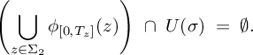
Finally, we fix a small constant
 $\epsilon _2>0$
and take
 $$ \begin{align} \kappa=\exp\big[\pi(p)\cdot(u_2+\epsilon_2)\big]. \end{align} $$
Similar to Claim 4.7, we can take an adapted
 $C^1$
-coordinate on
 $\Sigma _2$
, such that
 in this coordinate and the second and third items of the claim are satisfied on

See [Reference Shilnikov, Shilnikov, Turaev and Chua63, Theorem 2.4 & 2.5]. This finishes the proof of the claim.
Let  which is a neighborhood of
 $\operatorname {Orb}(p)$
. Since
 $W^u(\sigma )\setminus \{\sigma \}\subseteq W^s(\operatorname {Orb}(p))$
, for
 , there exist
 $T^\pm>0$
and
 such that
 $$ \begin{align*} (r^+,0)=\phi_{T^+}(z^+), \qquad \mathrm{and} \qquad (r^-,0)=\phi_{T^-}(z^-). \end{align*} $$
Since
 $\operatorname {Orb}^+(z^\pm )\cap U(\sigma )=\emptyset $
, there exist two constants
 $\delta _0>0,K>0$
with
 $K\cdot \delta _0\ll 1$
, such that
-
• The Poincaré map
$P^+:\Sigma ^+(\delta _0)\rightarrow \Sigma _p$
is well defined and
$C^1$
-smooth, satisfying
$P^+(z^+)=P^+(0,1)=(r^+,0)$
, and for every , if we denote
$P^+(w)=(r_w,s_w)$
, then it satisfies Moreover, if we denote
$$ \begin{align*} \|r_w-r^+\|\leq K\cdot\|x_w\|, \qquad \mathrm{and} \qquad \|s_w\|\leq K\cdot\|x_w\|. \end{align*} $$
$T^+_w>0$
the time satisfying
$P^+(w)=\phi _{T^+_w}(w)$
, then the orbit segment
$\phi _{(0,T^+_w)}(w)\cap U(\sigma )=\emptyset $
.
-
• The Poincaré map
$P^-:\Sigma ^-(\delta _0)\rightarrow \Sigma _p$
is well defined and
$C^1$
-smooth, satisfying
$P^-(z^-)=P^-(0,-1)=(r^-,0)$
, and for every , if we denote
$P^-(w)=(r_w,s_w)$
, then it satisfies Moreover, if we denote
$$ \begin{align*} \|r_w-r^-\|\leq K\cdot\|x_w\|, \qquad \mathrm{and} \qquad \|s_w\|\leq K\cdot\|x_w\|. \end{align*} $$
$T^-_w>0$
the time satisfying
$P^-(w)=\phi _{T^-_w}(w)$
, then the orbit segment
$\phi _{(0,T^-_w)}(w)\cap U(\sigma )=\emptyset $
.



 , if we denote








 , if we denote





Claim 4.10. For every  with
 $x_z\neq 0,y_z>0$
, let
 $T_1<0<T_2$
be defined as in Claim 4.8 and
 . Then for the point
 , let
 $$ \begin{align*} T_p=\left(-\frac{\log(K\|x_w\|)}{\log\kappa}-2\right)\cdot T_0. \end{align*} $$
We have
 $\phi _{[0,T_p]}(P^+(w))\subseteq V(p)$
.
In particular, combined with the third item of Claim 4.8 that
 $T_2-T_1\leq \log \|x_w\|/u_1$
, we have
 $$ \begin{align} \frac{T_p}{T_2-T_1}~\geq~ \frac{-u_1\cdot T_0}{\log\kappa}\cdot \left(1+\frac{\log K+2\log\kappa}{\log\|x_w\|}\right). \end{align} $$
The same conclusion holds for  with
 $x_z\neq 0,y_z<0$
.
Proof of Claim 4.10.
We only prove the case that
 $y_z>0$
. From the property of Poincaré map
 $P^+:\Sigma ^+(\delta _0)\to \Sigma _p$
, we have
 $\|s_w\|\leq K\cdot \|x_w\|$
. Moreover, for the Poincaré map
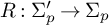 $R:\Sigma _p'\to \Sigma _p$
in the neighborhood of
 $\mathrm {Orb}(p)$
, we can apply the third item of Claim 4.9, which shows that for the point
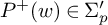 , it will iterate by R at least
 $([-\log \|s_w\|/\log \kappa ]-1)$
-times hitting
 $\Sigma _p'$
inside
 $V(p)$
. So for
 $$ \begin{align*} T_p~=~\left(-\frac{\log(K\|x_w\|)}{\log\kappa}-2\right)\cdot T_0 ~\leq~ \left(\left[\frac{\log\|s_w\|}{\log\kappa}\right]-1\right)\cdot T_0, \end{align*} $$
we have
 $\phi _{[0,T_p]}(P^+(w))\subseteq V(p)$
.
Moreover, by the fact
 $0<T_2-T_1\leq \log \|x_w\|/u_1$
, we have the following estimates:
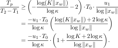 $$ \begin{align*} \frac{T_p}{T_2-T_1}&\geq \left(-\frac{\log(K\|x_w\|)}{\log\kappa}-2\right)\cdot T_0\cdot \frac{u_1}{\log\|x_w\|}\\ &= \frac{-u_1\cdot T_0}{\log \kappa}\left(\frac{\log(K\|x_w\|)+2\log\kappa}{\log\|x_w\|} \right)\\ &= \frac{-u_1\cdot T_0}{\log\kappa}\cdot \left(1+\frac{\log K+2\log\kappa}{\log\|x_w\|}\right). \end{align*} $$
This proves the claim.
Now we take  small enough, such that
 $(\log K+2\log \kappa )/\log \delta _1>-1/2$
. Then for every
 , the corresponding estimation of Equation (4.3) is
 $$ \begin{align} T_p~\geq~ L\cdot(T_2-T_1), \qquad \mathrm{where} \qquad L=\frac{-u_1\cdot T_0}{2\log\kappa}. \end{align} $$
Now we take a
 $C^1$
smooth function
 $\varphi :M\rightarrow {\mathbb R}$
satisfying:
-
1.
$\varphi (z)\geq -1$
for every and
$\varphi (\sigma )=-1$
. -
2.
$\varphi (z)\geq 0$
for every . -
3.
$\varphi (z)\geq L^{-1}$
for every .

 and


 .

 .
Then for the generic point
 $x_n$
of
 $\mu _n$
, let
 $$ \begin{align*} 0~\leq~ T_1^1<T_2^1<T_3^1<T_4^1~<~ \cdots\cdots ~<~T_1^m<T_2^m<T_3^m<T_4^m~<~\cdots\cdots \end{align*} $$
be the time sequence where
 $\{T_1^m\}_m$
are all the times that
 $\phi _t(x_n)$
enters
 $U(\sigma ,\delta _1)$
and
 $T_2^m$
is the time when
 $\phi _t(x_n)$
enters
 $U(\sigma ,\delta _1)$
after
 $T_1^m$
;
 $T_3^m$
is the time when
 $\phi _t(x_n)$
enters
 $V(p)$
after
 $T_2^m$
and
 $T_4^m$
is the time when
 $\phi _t(x_n)$
leaves
 $V(p)$
after
 $T_3^m$
.
For every m, we have
 $$ \begin{align*} (T_4^m-T_3^m)~\geq~L\cdot (T_2^m-T_1^m). \end{align*} $$
This implies
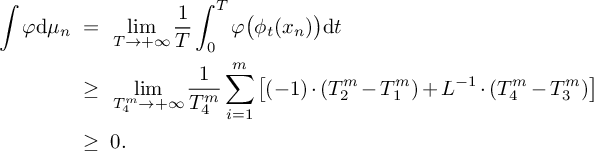
However, we have  . This contradicts
 $\mu _n\rightarrow \delta _\sigma $
; thus,
 $\delta _\sigma $
is isolated in
 $\mathcal {M}_{erg}(X)$
.
4.4 Proof of Theorem B and Corollary 1.4
We split the proof of Theorem B into two parts: the dense part and the residual part. We first give some preparations. The following proposition states that any ergodic measure supported on a singular hyperbolic homoclinic class can be accumulated by periodic measures if it is not supported on singularities.
Proposition 4.11. Let 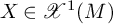 and
 $\Lambda $
be a singular hyperbolic homoclinic class. Assume
 is not an atomic measure supported on any singularity. Then
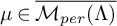 .
Remark 4.12. The proof of Proposition 4.11 originates from [Reference Crovisier23, Proposition 1.4] following Katok’s arguments [Reference Katok40] for the case of diffeomorphisms, while for vector fields, the arguments essentially follows [Reference Shi, Gan and Wen62, Theorem 5.6] by applying Liao’s shadowing lemma [Reference Liao43, Reference Liao44]. Thus, we omit the proof.
Next, we state the following two lemmas. Recall by Proposition 3.8, any geometric Lorenz attractor of a vector field  is a homoclinic class and any two periodic orbits are homoclinically related. Hence, we have the following lemma which is a combination of [Reference Abdenur, Bonatti and Crovisier1, Proposition 4.7 & Remark 4.6].
Lemma 4.13. Assume  and
 admits a geometric Lorenz attractor
 $\Lambda $
. Then
 $\overline {\mathcal {M}_{per}(\Lambda )}$
is convex.
The next lemma states that periodic measures are dense in the ergodic measure space of Lorenz attractors for
 $C^r$
-generic
 . Its proof is by a classical Baire argument, which we postpone in the end of this section.
Lemma 4.14. For every  , there exists a
 $C^r$
-residual subset
 $\mathcal {R}^r\subset \mathscr {X}^r(M^3)$
such that if
 admits a Lorenz attractor
 $\Lambda $
, then
 $\mathcal {M}_{erg}(\Lambda )\subset \overline {\mathcal {M}_{per}(\Lambda )}$
.
Now we manage to prove Theorem B and Corollary 1.4. In certain cases, we have to perturb a vector field in different open regions. The results in [Reference Pugh and Robinson57, Section 2] guarantee that every vector field  (
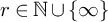 ) admits a basis of neighborhoods
 $\mathcal {U}$
satisfying the following property:
-
(F) : For any two perturbations
of X, if there exist two open sets
$W_1,W_2$
such that
$Y_i=X|_{M\setminus W_i}$
for
$i=1,2$
and
$W_1\cap W_2=\emptyset $
, then the composed perturbation Y is also in
$\mathcal {U}$
, where
$Y=X|_{M\setminus {W_1\cup W_2}}$
and
$Y=Y_i|_{W_i}$
for
$i=1,2$
.
 of X, if there exist two open sets

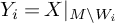






Proof of Theorem B. Let  . We split the proof of Theorem B into dense part and residual part.
Dense part:
By Proposition 3.8 and robustness of hyperbolic singularities, one can easily prove that there exists an open and dense subset
 $\mathcal {O}$
in
 $\mathscr {X}^r(M^3)$
such that the number of geometric Lorenz attractors of every
 is robustly constant. That is to say, for any
 , there exists a
 $C^r$
neighborhood
 $\mathcal {V}_X$
of X such that the number of geometric Lorenz attractors of any
 is a constant which equals that of X.
To prove the dense part, we only need to show that for any  and for any
 $C^r$
neighborhood
 $\mathcal {V}$
of X, there exists a vector field
 such that every geometric Lorenz attractor
 $\Lambda _Y$
of Y satisfies
 $$ \begin{align*}\overline{\mathcal{M}_{per}(\Lambda_Y)}\subsetneqq \overline{\mathcal{M}_{erg}(\Lambda_Y)}\subsetneqq \mathcal{M}_{inv}(\Lambda_Y).\end{align*} $$
By hyperbolicity of singularities, we have that X admits only finitely many geometric Lorenz attractors
 $\Lambda _1,\Lambda _2,\cdots ,\Lambda _k$
with pairwise disjoint attracting regions
 $U_1,U_2,\cdots ,U_k$
. Shrinking
 $\mathcal {V}$
if necessary, we assume that every
 admits exactly k geometric Lorenz attractors
 $\Lambda _{1,Z},\Lambda _{2,Z},\cdots ,\Lambda _{k,Z}$
with the same attracting regions
 $U_1,U_2,\cdots ,U_k$
. Moreover, we assume that
 $\mathcal {V}$
satisfies the property
 $(F)$
above. For each
 and for each
 $i=1,2,\cdots ,k$
, we denote by
 $\sigma _i^{Z}$
the unique singularity in
 $\Lambda _{i,Z}$
and denote by
 $\sigma _i=\sigma _i^{X}$
for simplicity. We first show the following claim.
Claim 4.15. For each
 $i=1,2,\cdots ,k$
, there exists
 satisfying that
 $Y_i|_{M\setminus U_i}=X|_{M\setminus U_i}$
and
 $W^u(\sigma _i^{Y_i},\phi _t^{Y_i})\setminus \{\sigma _i^{Y_i}\}\subset W^s(\operatorname {Orb}(p_i^{Y_i},\phi _t^{Y_i}))$
, where
 $p_i^{Y_i}$
is a hyperbolic periodic point of
 $\phi _t^{Y_i}$
.
Proof of Claim 4.15.
Fix  . We denote by
 $\Lambda =\Lambda _i,U=U_i$
and
 $\sigma =\sigma _i$
to simplify notations.
Let
 $\Sigma \subset U$
be the cross section of
 $\Lambda $
and
 be the two different points satisfying
 $\phi _t^X(z^+),\phi _t^X(z^-)\notin \Sigma $
for any
 $t<0$
. Take a hyperbolic periodic point
 . Take a constant
 $\delta ^+>0$
such that
-
•
$B(z^{+},\delta ^+)\subset U\setminus (\operatorname {Orb}(p,\phi ^X_t)\cup \{\sigma \})$
, -
•
$\phi ^X_t(z^-)\notin B(z^{+},\delta ^+)$
for any
$t\leq 0$
.



By Theorem 3.10, there exists  satisfying that
 $$ \begin{align*}Y^+|_{M\setminus B(z^{+},\delta^+)}=X|_{M\setminus B(z^{+},\delta^+)} \text{~~and~~} \operatorname{Orb}(z^+,\phi_t^{Y^+})\subset W^u(\sigma,\phi_t^{Y^+})\cap W^s(\operatorname{Orb}(p),\phi_t^{Y^+}).\end{align*} $$
Note that
 $\mathcal {V}$
is also a
 $C^r$
-neighborhood of
 $Y^+$
with
 and
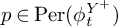 . Moreover, by the choice of
 $\mathcal {V}$
, the maximal invariant compact set of
 $\phi ^{Y^+}_t$
is still a geometric Lorenz attractor with singularity
 $\sigma $
and containing
 $\operatorname {Orb}(p)$
in it. We take another constant
 $\delta ^->0$
satisfying that
-
•
$B(z^{-},\delta ^-)\subset U\setminus (\operatorname {Orb}(p,\phi ^X_t)\cup \{\sigma \})$
, -
•
$\phi ^{Y^+}_t(z^+)\notin B(z^{-},\delta ^-)$
for any .


 .
Applying Theorem 3.10 again for the vector field
 $Y^+$
and the neighborhood
 $\mathcal {V}$
, there exists
 such that
 $$ \begin{align*}Y_i|_{M\setminus B(z^{-},\delta^-)}=Y^+|_{M\setminus B(z^{-},\delta^-)} \text{~~and~~} \operatorname{Orb}(z^-,\phi_t^{Y_i})\subset W^u(\sigma,\phi_t^{Y_i})\cap W^s(\operatorname{Orb}(p),\phi_t^{Y_i}).\end{align*} $$
By the choice of
 $\delta ^-$
, we know that it satisfies also
 $$ \begin{align*}\operatorname{Orb}(z^+,\phi_t^{Y_i})\subset W^u(\sigma,\phi_t^{Y_i})\cap W^s(\operatorname{Orb}(p),\phi_t^{Y_i}).\end{align*} $$
The vector field
 $Y_i$
satisfies Claim 4.15.
Finally, let Y be the composed perturbation of X satisfying that
 $$ \begin{align*}Y|_{U_i}=Y_i|_{U_i}, ~\text{ for each~} i=1,2,\cdots,k,~~~\text{ and~~~} Y|_{M\setminus (\bigcup_{1\leq i\leq k}U_i)}=X|_{M\setminus (\bigcup_{1\leq i\leq k}U_i)}.\end{align*} $$
By the property
 $(F)$
, we have that
 since the attracting regions
 $\{U_i\}_{1\leq i\leq k}$
are pairwise disjoint. By Proposition 4.5, for each
 $1\leq i\leq k$
, the Dirac measure
 $\delta _{\sigma _i}=\delta _{\sigma _i^Y}$
is isolated in
 $\mathcal {M}_{erg}(Y)$
. In particular, we have
 $$ \begin{align*}\overline{\mathcal{M}_{per}(\Lambda_{i,Y})}\subsetneqq \overline{\mathcal{M}_{erg}(\Lambda_{i,Y})}\subsetneqq \mathcal{M}_{inv}(\Lambda_{i,Y}).\end{align*} $$
The proof of dense part is completed.
Residual part:
Let
 $\mathcal {R}^r\subset \mathscr {X}^r(M^3)$
be the residual subset from Lemma 4.14. Assume
 admits a geometric Lorenz attractor
 $\Lambda $
. We first show that
 $$ \begin{align*}\mathcal{M}_{inv}(\Lambda)=\overline{\mathcal{M}_{erg}(\Lambda)}=\overline{\mathcal{M}_{per}(\Lambda)}.\end{align*} $$
Take  . By the Ergodic Decomposition Theorem, there exists a sequence of measures
 $\mu _n$
converging to
 $\mu $
in the weak*-topology where
 is a convex sum of finitely many ergodic measures supported on
 $\Lambda $
for each
 . By Lemma 4.14, there exists a sequence of measures
 $\nu _n$
converging to
 $\mu $
in the weak*-topology where
 is a convex sum of finitely many periodic measures supported on
 $\Lambda $
for each
 . By Lemma 4.13, we have that
 $\overline {\mathcal {M}_{per}(\Lambda )}$
is convex. Hence,
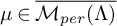 . This implies
 $\mathcal {M}_{inv}(\Lambda )=\overline {\mathcal {M}_{erg}(\Lambda )}=\overline {\mathcal {M}_{per}(\Lambda )}$
.
Note that
 $\mathcal {M}_{erg}(\Lambda )$
coincides with
 $\overline {\mathcal {M}_{per}(\Lambda )}\cap \mathcal {M}_{erg}(\Lambda )$
. Hence, the path connectedness of
 $\mathcal {M}_{erg}(\Lambda )$
follows directly from Proposition 3.8 and Proposition 4.1. This completes the residual part and hence the proof of Theorem B.
Proof of Corollary 1.4.
Let
 $\mathcal {R}^r$
be the residual subset of
 $\mathscr {X}^r(M^3)$
from Theorem B. Assume
 admits a geometric Lorenz attractor
 $\Lambda $
. By [Reference Abdenur, Bonatti and Crovisier1, Proposition 5.1],
 $\mathcal {M}_{erg}(\Lambda )$
is a
 $G_{\delta }$
subset in
 $\mathcal {M}_{inv}(\Lambda )$
. Since
 $\mathcal {M}_{inv}(\Lambda )=\overline {\mathcal {M}_{erg}(\Lambda )}$
, we have that
 $\mathcal {M}_{erg}(\Lambda )$
is a residual subset in
 $\mathcal {M}_{inv}(\Lambda )$
. However, periodic orbits are dense in
 $\Lambda $
since
 $\Lambda $
is a homoclinic class. Then by [Reference Abdenur, Bonatti and Crovisier1, Proposition 5.3], the set of invariant measures with support equal to
 $\Lambda $
is a residual subset
 $\mathcal {M}_1$
in
 $\mathcal {M}_{inv}(\Lambda )$
. By [Reference Pacifico, Yang and Jang53], the entropy map
 $$ \begin{align*}h_{(\cdot)}\colon \mathcal{M}_{inv}(\Lambda)\rightarrow \mathbb{R}\end{align*} $$
 $$ \begin{align*}~~~~~~~~~~\mu\mapsto h_{\mu}(X)\end{align*} $$
is upper semi-continuous. Hence, the continuity points of the entropy map
 $h_{(\cdot )}$
form a residual subset
 $\mathcal {M}_2$
in
 $\mathcal {M}_{inv}(\Lambda )$
. Moreover, since
 $\mathcal {M}_{inv}(\Lambda )=\overline {\mathcal {M}_{per}(\Lambda )}$
and every periodic measure has
 $0$
-entropy, we have that every
 satisfies
 $h_{\mu }(X)=0$
. Let
 $$ \begin{align*}\mathcal{M}_{res}=\mathcal{M}_{erg}(\Lambda)\cap \mathcal{M}_1\cap \mathcal{M}_2.\end{align*} $$
Then
 $\mathcal {M}_{res}$
is a residual subset in
 $\mathcal {M}_{inv}(\Lambda )$
, and the residual part concludes.
To prove the dense part, since
 $\mathcal {M}_{inv}(\Lambda )=\overline {\mathcal {M}_{per}(\Lambda )}$
, we only need to show that any periodic measure supported on
 $\Lambda $
is approximated by ergodic measures in
 $\mathcal {M}_{erg}(\Lambda )$
with positive entropy. The idea follows [Reference Abdenur, Bonatti and Crovisier1, Theorem 3.5 part (c)], and we give an explanation here. For any periodic orbit
 $\operatorname {Orb}(p)$
in
 $\Lambda $
, we have that
 $\Lambda =H(p)$
by Proposition 3.8. Hence,
 $\operatorname {Orb}(p)$
exhibits some transverse homoclinic orbit which implies that there are hyperbolic horseshoes contained in
 $\Lambda $
arbitrarily close to this homoclinic orbit. That means points in the hyperbolic horseshoes spends arbitrarily large fractions of their orbits shadowing
 $\operatorname {Orb}(p)$
as closely as required. Hence, measures supported on such hyperbolic horseshoes are close to
 $\delta _{\operatorname {Orb}(p)}$
in the weak*-topology. However, every hyperbolic horseshoe must support an ergodic measure with positive entropy. Thus,
 $\delta _{\operatorname {Orb}(p)}$
is approximated by ergodic measures in
 $\mathcal {M}_{erg}(\Lambda )$
with positive entropy.
Remark 4.16. In the proof of Corollary 1.4, the residual subsets
 $\mathcal {M}_1$
and
 $\mathcal {M}_2$
of
 $\mathcal {M}_{inv}(\Lambda )$
exist for every geometric Lorenz attractor
 $\Lambda $
of every
 . Therefore, the measures with zero entropy and full support form a residual subset
 $\mathcal {M}_0$
in
 $\mathcal {M}_{inv}(\Lambda )$
for every geometric Lorenz attractor
 $\Lambda $
. Here is an explanation:
First, periodic points are dense in
 $\Lambda $
since it is a homoclinic class by Proposition 3.8. By [Reference Abdenur, Bonatti and Crovisier1, Proposition 5.3], the set of invariant measures with full support is a residual subset
 $\mathcal {M}_1$
in
 $\mathcal {M}_{inv}(\Lambda )$
. Second, by Proposition 4.11, the set
 $\mathcal {M}_{per}(\Lambda )\cup \{\delta _{\sigma }\}$
is dense in
 $\mathcal {M}_{erg}(\Lambda )$
. This implies that every
 is the limit of invariant measures
 $\{\mu _n\}$
, where each
 $\mu _n$
is the convex sum of finitely many periodic measures supported on
 $\Lambda $
together with
 $\delta _{\sigma }$
. Thus, by the upper semi-continuity of the entropy map [Reference Pacifico, Yang and Jang53], the invariant measures with zero entropy form a residual subset
 $\mathcal {M}_2$
in
 $\mathcal {M}_{inv}(\Lambda )$
.
To end this section, we prove Lemma 4.14.
Proof of Lemma 4.14.
Assume  admits a Lorenz attractor
 $\Lambda $
with attracting region U and let
 $\mathcal {U}$
be the
 $C^r$
neighborhood of X satisfying Proposition 3.8 for
 $\Lambda $
and U. Recall that
 $\Lambda $
is a homoclinic class and any two periodic orbits are homoclinically related by Proposition 3.8. Applying Corollary 3.11 and Proposition 4.4, we have the following claim.
Claim 4.17. For any
 $C^r$
-neighborhood
 $\mathcal {V}$
of X and any
 $\varepsilon>0$
, there exists
 which admits a periodic point p satisfying that
 $d(\delta _{\operatorname {Orb}(p,\phi ^Y_t)},\delta _{\sigma _Y})<\varepsilon $
.
Lemma 4.14 concludes by a standard Baire argument. Take a countable basis  of
 $M^3$
and let
 be the countable family which consists of all the possible unions of finitely many elements in
 . For each pair of integers
 , we define the following two subsets of
 $\mathscr {X}^r(M^3)$
:
-
•
$\mathcal {F}_{m,n}$
: if and only if Y admits a hyperbolic singularity
$\sigma _Y$
in
$U_m$
and there exists a periodic point
$q_Y$
of Y such that
$d(\delta _{\operatorname {Orb}(q_Y,\phi ^Y_t)},\delta _{\sigma _Y})<\frac {1}{n}$
; -
•
$\mathcal {N}_{m,n}$
: if and only if there exists a neighborhood
$\mathcal {V}_Y\subset \mathscr {X}^r(M^3)$
of Y such that for any , one of the following cases satisfies-
– either Z admits no hyperbolic singularity in
$U_m$
; -
– or for any singularity
$\sigma _Z$
of Z in
$U_m$
and for any periodic point
$q_Z$
of Z, it satisfies
$d(\delta _{\operatorname {Orb}(q_Z,\phi ^Z_t)},\delta _{\sigma _Z})\geq \frac {1}{n}$
.
-

 if and only if Y admits a hyperbolic singularity




 if and only if there exists a neighborhood

 , one of the following cases satisfies



Claim 4.18.
 $\mathcal {F}_{m,n}\cup \mathcal {N}_{m,n}$
is open and dense in
 $\mathscr {X}^r(M^3)$
.
Proof. By the robustness of hyperbolic critical elements, we have that
 $\mathcal {F}_{m,n}$
is open in
 $\mathscr {X}^r(M^3)$
. The openness of
 $\mathcal {N}_{m,n}$
is by definition.
For any vector field  , there exists a sequence of vector fields
 such that
 $Y_i$
admits a hyperbolic singularity
 $\sigma _{Y_i}$
in
 $U_m$
, and there exists a periodic point
 $q_{Y_i}$
of
 $Y_i$
such that
 $d(\delta _{\operatorname {Orb}(q_{Y_i})},\delta _{\sigma _{Y_i}})<\frac {1}{n}$
. Again by the robustness of hyperbolic critical elements, we have that
 , which implies that
 . This shows that
 $\mathcal {F}_{m,n}\cup \mathcal {N}_{m,n}$
is dense in
 $\mathscr {X}^r(M^3)$
.
By Claim 4.18, the set
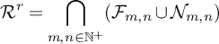
is a residual subset in
 $\mathscr {X}^r(M^3)$
. Let
 and
 $\Lambda $
be a Lorenz-like attractor of X with singularity
 $\sigma $
. We show that
 $\mathcal {M}_{erg}(\Lambda )\subset \overline {\mathcal {M}_{per}(\Lambda )}$
.
Take  . If
 $\mu \neq \delta _{\sigma }$
, then
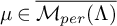 by Proposition 4.11. Otherwise
 $\mu =\delta _\sigma $
. By the hyperbolicity of
 $\sigma $
, there exist a neighborhood
 $U_\sigma $
of
 $\sigma $
and a neighborhood
 $\mathcal {U}_X\subset \mathscr {X}^r(M^3)$
of X such that any
 admits a unique singularity
 $\sigma _Z$
in
 $U_\sigma $
where
 $\sigma _Z$
is the continuation of
 $\sigma $
. Take
 such that
 $U_m\subset U_{\sigma }$
is a neighborhood of
 $\sigma _Z$
for all
 . By Claim 4.17, we have that
 $X\notin \mathcal {N}_{m,n}$
for any
 . Hence,
 for any
 . This implies that there exists a sequence of periodic points
 $p_n$
of X such that
 $\delta _{\operatorname {Orb}(p_n)}$
converges to
 $\delta _{\sigma }$
in the weak*-topology. Moreover, since
 $\Lambda $
is a Lorenz attractor, we have that
 for each n large enough. This shows that
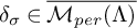 and completes the proof of Lemma 4.14.
A Appendix: Robustness of geometric Lorenz attractors
In Appendix A, we prove Proposition 3.8, which shows the geometric Lorenz attractor is a homoclinic class and the vector fields exhibiting a geometric Lorenz attractor forms a
 $C^2$
-open subset in
 $\mathscr {X}^r(M^3)$
for every
 .
Proof of Proposition 3.8.
The proof of
 $\Lambda $
is a homoclinic class, and every two periodic orbits of
 $\Lambda $
are homoclinic relies on the fact that the one-dimensional quotient map f is eventually onto (Lemma 3.6). We refer to [Reference Bautista8, Theorem 1] for showing that
 $\Lambda $
is a homoclinic class. For every two periodic points
 , we can assume
 . Let
 $\gamma ^u\subset W^u_{\mathit {loc}}(\operatorname {Orb}(p),\phi _t^X)\cap \Sigma $
be the segment containing p in
 $\Sigma $
. Let
 . Then
 $\{x_q\}\times [-1,1]\subset W^s_{\mathit {loc}}(\operatorname {Orb}(q),\phi _t^X)$
. We only need to show there exists some
 $n>0$
such that
 $$ \begin{align*} P^n(\gamma^u)~\cap~\{x_q\}\times[-1,1]~\neq~\emptyset. \end{align*} $$
Here,
 $P:\Sigma \setminus l\rightarrow \Sigma $
is the Poincaré map. Let
 $J=\pi _x(\gamma ^u)$
. This is equivalent to
 $n>0$
existing such that
 , which has been proved in Lemma 3.6.
Now we prove the second part of this proposition. We only need to show for every  which exhibits a geometric Lorenz attractor with attracting region U, there exists a
 $C^2$
-neighborhood
 $\mathcal {U}$
of X, such that for every
 , the maximal invariant set
 $\Lambda _Y=\bigcap _{t>0}\phi _t^Y(U)$
is a geometric Lorenz attractor.
Let
 $\lambda _0>\sqrt {2}$
be the constant fixed in Notation 3.4 satisfying
 $f'(x)>\lambda _0$
for every
 . Let
 $\eta>0$
be a fixed constant satisfying

Since
 $U\subseteq M^3$
is an attracting region of X and
 $\Lambda =\bigcap _{t>0}\phi _t^X(U)$
is singular hyperbolic
 $T_{\Lambda }M^3=E^{ss}\oplus E^{cu}$
, there exists a
 $C^2$
-neighborhood
 $\mathcal {U}_1$
of X, such that for every
 , U is an attracting region of Y and
 $\Lambda _Y=\bigcap _{t>0}\phi _t^Y(U)$
is singular hyperbolic with splitting
 $T_{\Lambda _Y}M^3=E^{ss}_Y\oplus E^{cu}_Y$
. Moreover, the singularity
 also has three eigenvalues
 $\lambda _{1,Y}<\lambda _{2,Y}<0<\lambda _{3,Y}$
satisfying
 $\lambda _{1,Y}+\lambda _{3,Y}<0$
and
 $\lambda _{2,Y}+\lambda _{3,Y}>0$
for every
 .
Let
 $\Sigma =[-1-\epsilon ,1+\epsilon ]^2$
be the cross section of X and
 $\Lambda $
defined in Lemma 3.2. By the continuity of the singularity
 $\sigma _Y$
and the continuity of the local stable and unstable manifolds of
 $\sigma _Y$
, shrinking
 $\mathcal {U}_1$
if necessary, we can further assume that for every
 , it satisfies
-
1. For every
, there exists
$T>0$
, such that . -
2. The local stable manifold of
$\sigma _Y$
intersects
$\Sigma $
with
$l_Y=W^s_{\mathit {loc}}(\sigma _Y,\phi _t^Y)\cap \Sigma $
being
$C^2$
-close to
$l=\{0\}\times [-1-\epsilon ,1+\epsilon ]$
. -
3. The unstable manifold of
$\sigma _Y$
intersects
$\Sigma $
with which are close to
$z^+,z^-$
, respectively. -
4. The Poincaré map
$P_Y:\Sigma \setminus l_Y\rightarrow \Sigma $
is well defined and satisfies
$$ \begin{align*} \overline{P_Y(\Sigma\setminus l_Y)}~=~ P_Y(\Sigma\setminus l_Y)\cup\{z_Y^+,z_Y^-\}~\subseteq~ \mathrm{Int}(\Sigma). \end{align*} $$
-
5. For every
, we have
$$ \begin{align*} \frac{\partial\pi_x\circ P_Y}{\partial x}(x,y)>(1+\eta)^{-1}\lambda_0, \quad \frac{\partial\pi_y\circ P_Y}{\partial x}(x,y)<(1+\eta)^{-3}, \!\quad \mathrm{and} \!\!\quad \frac{\partial\pi_y\circ P_Y}{\partial y}(x,y)<1. \end{align*} $$
 , there exists

 .







 which are close to



 , we have

For every  , we denote
 $\mathcal {F}^{ss}_Y$
the strong stable foliation of Y tangent to
 $E^{ss}_Y$
in U, and
 the 2-dimensional stable foliation in
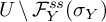 $U\setminus \mathcal {F}^{ss}_Y(\sigma _Y)$
defined as Lemma 3.1. Let
 $$ \begin{align*} \mathcal{F}^s_{Y,\Sigma}~=~\mathcal{F}^s_Y~\cap~\Sigma \end{align*} $$
be the stable foliation on
 $\Sigma $
induced by
 $\mathcal {F}^s_Y$
. By the classical stable manifold theorem [Reference Hirsch, Pugh and Shub39], for every
 , the leaf
 $\mathcal {F}^s_{Y,\Sigma }(z)$
converges to
 $\{x_z\}\times [-1-\epsilon ,1+\epsilon ]$
in
 $C^2$
-topology as
 $Y\rightarrow X$
in
 $\mathscr {X}^2(M^3)$
. To be precise, shrinking
 $\mathcal {U}$
if necessary, for every
 , there exists a
 $C^2$
-smooth function
 $\varphi ^s_z:[-1-\epsilon ,1+\epsilon ]\rightarrow (-\epsilon /2,\epsilon /2)$
, such that

The function
 $\varphi ^s_z$
satisfies
 $\varphi ^s_z(y_z)=0$
and
 $\varphi ^s_z\rightarrow 0$
in
 $C^2$
-topology as
 $Y\rightarrow X$
in
 $\mathscr {X}^2(M^3)$
.
Let
 $h^s_{Y,\Sigma }$
be the holonomy map induced by
 $\mathcal {F}^s_{Y,\Sigma }$
on
 $\Sigma $
. Now we show
 $h^s_{Y,\Sigma }$
converges to the holonomy map of the foliation
 in
 $C^1$
-topology.
Claim A.1. The holonomy map
 $h^s_{Y,\Sigma }$
is
 $C^{1+}$
-smooth on
 $\Sigma $
. There exists a
 $C^2$
-neighborhood
 $\mathcal {U}_2$
of X, such that for every
 and every two points
 ,
 $i=1,2$
. Let
 $$ \begin{align*} J_i=(a_i,b_i)\times\{y_i\}~\subset~ [-1-\epsilon/2,1+\epsilon/2]\times[-1-\epsilon,1+\epsilon] \end{align*} $$
be two intervals containing  , such that
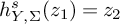 $h^s_{Y,\Sigma }(z_1)=z_2$
and
 $h^s_{Y,\Sigma }(J_1)=J_2$
. Then
 $$ \begin{align*} (1+\eta)^{-1}~<~ Dh^s_{Y,\Sigma}(z_1) ~<~(1+\eta). \end{align*} $$
This implies
 $h^s_{Y,\Sigma }$
converges to
 $h^s_{X,\Sigma }\equiv \mathrm {Id}_x$
in
 $C^1$
-topology as Y converges to X in
 $\mathscr {X}^2(M^3)$
.
Proof of the claim.
Due to a beautiful observation in [Reference Araújo and Melbourne3, Lemma 7.1], the holonomy map
 $h^s_Y$
of the stable foliation
 $\mathcal {F}^s_{Y,\Sigma }$
is
 $C^{1+}$
-smooth in the cross section
 $\Sigma $
. The key fact is that
 $h^s_Y$
is absolutely continuous with respect to the transversal Lebesgue measure. Thus, the fact that
 $\mathcal {F}^s_{Y,\Sigma }$
is codimension one implies
 $h^s_Y$
is
 $C^{1+}$
-smooth. Following the estimation in [Reference Araújo and Melbourne3, Lemma 7.1], we can show that the holonomy map
 $h^s_Y$
converges to
 $h^s_X$
in
 $C^1$
-topology as
 $Y\rightarrow X$
in
 $\mathscr {X}^2(M^3)$
.
Recall that the stable foliation
 $\mathcal {F}^{ss}_Y$
is Hölder continuous. There exists a Hölder continuous function
 $T:J_2\rightarrow {\mathbb R}$
, such that for every
 and
 , they satisfy

Here, we can assume the function
 $|T|<1$
on
 $J_2$
by flowing the cross section
 $\Sigma $
.
Since the strong stable foliation
 $\mathcal {F}^{ss}_Y$
is preserved by
 $\phi _t^Y$
, for t small enough, we have

This implies there exists
 $\delta>0$
, such that if
 $$ \begin{align*} I_{\delta}~=~[x_1-\delta,x_1+\delta]\times\{y_1\} ~\subset~(a_1,b_1)\times\{y_1\}~=~J_1, \end{align*} $$
and  , then the holonomy map of the local strong stable foliation
 $\mathcal {F}^{ss}_Y$
is well defined,

and satisfies
 $h^{ss}_Y(w_1)=\phi _{T(w_2)}^X(w_2)$
where
 .
The holonomy map
 $h^{ss}_Y:D^Y_{\delta }\rightarrow D^Y_2$
is absolutely continuous; see [Reference Brin and Pesin19, Reference Pugh and Shub59]. Moreover, let
 $m_1$
and
 $m_2$
be Lebesgue measures induced by the Riemannian metric restricted on
 $D^Y_{\delta }$
and
 $D^Y_2$
, respectively. Then for every
 and
 , the Jacobian of
 $h^{ss}_Y(w_1)$
is
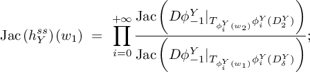
see [Reference Pesin58, Theorem 7.1 & Remark 7.2]. Notice here the infinite product must convergence since  .
For every
 $\kappa>0$
, there exists a
 $C^2$
-neighborhood
 $\mathcal {V}_{\kappa ,1}\subset \mathscr {X}^2(M^3)$
of X, and an integer
 $k>0$
, such that for every
 and
 $w_2=h^{ss}_Y(w_1)$
with
 , they satisfy

Here, we use the fact that the distance between
 $\phi _i^Y(w_1)$
and
 $\phi _i^Y(w_2)$
, and the distance between the tangent bundles
 $T_{\phi _i^Y(w_1)}\phi _i^Y(D^Y_{\delta })$
and
 $T_{\phi _i^Y(w_2)}\phi _i^Y(D^Y_2)$
, are both exponential convergent to zero.
For every  and every
 , we denote
 and
 for
 . Let
 $w_2^X=h^{ss}_X(w_t^X)$
and
 $w_2^Y=h^{ss}_Y(w_t^Y)$
. Equation A.2 and Equation A.3 show that
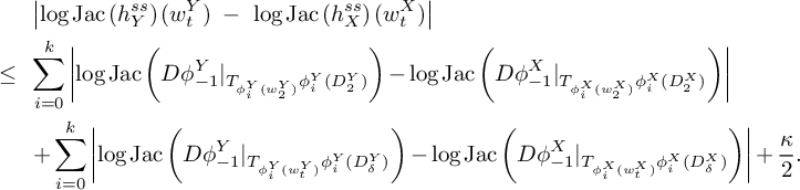 $$ \begin{align*} &\left| \log\operatorname{Jac}\left(h^{ss}_Y\right)(w_t^Y)~-~ \log\operatorname{Jac}\left(h^{ss}_X\right)(w_t^X) \right| \\ ~\leq~&\sum_{i=0}^{k} \left|\log\operatorname{Jac}\left(D\phi_{-1}^Y|_{T_{\phi_i^Y(w_2^Y)}\phi_i^Y(D^Y_2)}\right)- \log\operatorname{Jac}\left(D\phi_{-1}^X|_{T_{\phi_i^X(w_2^X)}\phi_i^X(D^X_2)}\right)\right| \\ &+\sum_{i=0}^{k} \left|\log\operatorname{Jac}\left(D\phi_{-1}^Y|_{T_{\phi_i^Y(w_t^Y)}\phi_i^Y(D^Y_{\delta})}\right)- \log\operatorname{Jac}\left(D\phi_{-1}^X|_{T_{\phi_i^X(w_t^X)}\phi_i^X(D^X_{\delta})}\right)\right|+\frac{\kappa}{2}. \end{align*} $$
When
 $Y\rightarrow X$
in
 $C^2$
-topology, we have
 $D\phi _{-1}^Y\rightarrow D\phi _{-1}^X$
, and for every
 $i=0,\cdots ,k$
,
-
•
$\phi _i^Y\big (D^Y_{\delta }\big )\rightarrow \phi _i^X\big (D^X_{\delta }\big )$
and
$\phi _i^Y\big (D^Y_2\big )\rightarrow \phi _i^X\big (D^X_2\big )$
in
$C^1$
-topology; -
•
$\phi _i^Y\big (w_t^Y\big )\rightarrow \phi _i^X\big (w_t^X\big )$
and
$\phi _i^Y\big (w_2^Y\big )\rightarrow \phi _i^X\big (w_2^X\big )$
.





So there exists a
 $C^2$
-neighborhood
 $\mathcal {V}_{\kappa ,2}\subset \mathcal {V}_{\kappa ,1}$
of X, such that for every
 ,
 $$ \begin{align*} \left| \log\operatorname{Jac}\left(h^{ss}_Y\right)(w_t^Y)~-~ \log\operatorname{Jac}\left(h^{ss}_X\right)(w_t^X) \right|<\kappa. \end{align*} $$
Thus we have
 $\operatorname {Jac}\left (h^{ss}_Y\right )\rightarrow \operatorname {Jac}\left (h^{ss}_X\right )$
as
 $Y\rightarrow X$
in
 $\mathscr {X}^2(M^3)$
.
Let  be the coordinate on
 $D_{\delta }^Y$
, which is defined as
 $w=(x,t)$
if
 and
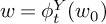 $w=\phi _t^Y(w_0)$
. Then there exists a smooth function
 $v^Y_1$
on
 $D_{\delta }^Y$
, such that the Lebesgue measure
 $m_1$
on
 $D_{\delta }^Y$
induced by the Riemannian metric is
 $$ \begin{align*} m_1(x,t)~=~v^Y_1(x,t)\mathrm{d}x\mathrm{d}t. \end{align*} $$
Similarly, we have the coordinate  on
 $D_2$
and the smooth function
 $v^Y_2$
satisfying the Lebesgue measure
 $m_2(x,t)=v^Y_2(x,t)\mathrm {d}x\mathrm { d}t$
on
 $D_2^Y$
.
According to the proof of [Reference Araújo and Melbourne3, Lemma 7.1], for every  and
 , let
 . Then
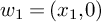 $w_1=(x_1,0)$
in the
 $(x,t)$
-coordinate in
 $D^Y_{\delta }$
, and
 $h^{ss}_Y(w_1)=\phi _{T(w_2^Y)}^Y(w_2)=(x_2,T(w_2^Y))$
in the
 $(x,t)$
-coordinate in
 $D^Y_2$
. The derivate of the holonomy map
 $h^s_{Y,\Sigma }$
is equal to

When
 $Y\rightarrow X$
in
 $\mathscr {X}^2(M^3)$
,
 $h^{ss}_Y(w_1)\rightarrow h^{ss}_X(w_1)$
, so
 $x_2^Y\rightarrow x_2^X$
and
 $T(w_2^Y)\rightarrow T(w_2^X)$
. Moreover,
 $D^Y_{\delta }\rightarrow D^X_{\delta }$
and
 $D^Y_2\rightarrow D^X_2$
imply
 $v^Y_i\rightarrow v^X_i$
for
 $i=1,2$
. Thus, Equation A.4 implies
 $$ \begin{align*} Dh^s_{Y,\Sigma}\longrightarrow Dh^s_{X,\Sigma}\equiv\mathrm{Id}_x \qquad \mathrm{as} \qquad Y\longrightarrow X~\mathrm{in}~\mathscr{X}^2(M^3). \end{align*} $$
Thus, for
 $\eta>0$
decided in (A.1), there exists a
 $C^2$
-neighborhood
 $\mathcal {U}_2$
of X, such that for every
 , it satisfies
 $$ \begin{align*} (1+\eta)^{-1}~<~ Dh^s_{Y,\Sigma} ~<~(1+\eta). \end{align*} $$
This finishes the proof of Claim A.1.
For every  , we give a new coordinate
 $\{(x',y')\}$
on the cross section
 $\Sigma $
, such that the Poincaré map of
 $\phi _t^Y$
associated to
 $\Sigma $
satisfies the definition of Lorenz attractors in this coordinate. For every
 , we fix the
 $y'$
-coordinate of z to
 $y^{\prime }_z=y_z$
.
For
 $\eta>0$
defined in (A.1), there exists
 $\epsilon _{\eta }>0$
, such that for every
 satisfying
 $$ \begin{align*} |x^--(-1)|<\epsilon_{\eta}, \qquad |x^+-1|<\epsilon_{\eta}, \qquad \mathrm{and} \qquad |x_0|<\epsilon_{\eta}, \end{align*} $$
there exists a diffeomorphism
 $h:{\mathbb R}\rightarrow {\mathbb R}$
satisfying

The unstable manifolds of
 $\sigma _Y$
intersect
 $\Sigma $
with
 $z^+_Y\rightarrow z^+=(-1,y^+)$
and
 $z^-_Y\rightarrow z^-=(1,y^+)$
as
 $Y\rightarrow X$
. Moreover, the intersection between the local stable manifolds of
 $\sigma _Y$
and
 $\Sigma $
satisfies
 $W^s_{\mathit {loc}}(\sigma _Y,\phi _t^Y)\cap \Sigma =l_Y\rightarrow l=\{0\}\times [-1-\epsilon ,1+\epsilon ]$
as
 $Y\rightarrow X$
. There exists a
 $C^2$
-neighborhood
 $\mathcal {U}_3$
of X, such that for every
 , let
 $\mathcal {F}^s_{Y,\Sigma }$
be the stable foliation on
 $\Sigma $
and
 $J_0=[-1-\epsilon ,1+\epsilon ]\times \{0\}$
. Then the coordinates
 $$ \begin{align*} \mathcal{F}^s_{Y,\Sigma}(z^+_Y)\cap J_0=(x^-_Y,0), \quad \mathcal{F}^s_{Y,\Sigma}(z^-_Y)\cap J_0=(x^+_Y,0), \quad \mathrm{and} \quad l_Y\cap J_0=(x_{0,Y},0) \end{align*} $$
satisfy
 $$ \begin{align*} |x^-_Y-(-1)|<\epsilon_{\eta}, \qquad |x^+_Y-1|<\epsilon_{\eta}, \qquad \mathrm{and} \qquad |x_{0,Y}|<\epsilon_{\eta}. \end{align*} $$
Let
 $h_Y:{\mathbb R}\rightarrow {\mathbb R}$
be the diffeomorphism satisfying

Then we define
 $x'$
-coordinate on
 $J_0$
as following: for every
 , the
 $(x',y')$
-coordinate of z is
 $$ \begin{align*} (~x^{\prime}_z,~y^{\prime}_z~)~=~\big(~h_Y(x_z),~0~\big). \end{align*} $$
Let
 $J_Y=\{(x,0):~-1\leq h_Y(x)\leq 1\}\subseteq J_0$
, and

For every  , let
 $w=(x_w,0)=\mathcal {F}^s_{Y,\Sigma }(z)\cap J_0$
. Then we define the
 $x'$
-coordinate of z as
 $$ \begin{align*} (~x^{\prime}_z,~y^{\prime}_z~)~=~(~x^{\prime}_w,~y_z~)~=~\big(~h_Y(x_w),~y_z~\big). \end{align*} $$
Thus, in the coordinate
 $\big \{(x',y')\big \}$
,
 $\Sigma _Y$
is
 $C^1$
-diffeomorphic to
 $[-1,1]^2$
.
For every  , the stable foliation
 $\mathcal {F}^s_{Y,\Sigma }$
is invariant under the action of Poincaré map; hence, the Poincaré map
 $P_Y:\Sigma _Y\setminus l_Y\rightarrow \Sigma _Y$
is well defined and has the form

From the construction of
 $(x',y')$
-coordinate on
 $\Sigma _Y$
, the one-dimensional quotient map
 $f_Y$
is
 $C^1$
-smooth and satisfies
 $\lim _{x'\rightarrow 0^-}f_Y(x')=1$
,
 $\lim _{x'\rightarrow 0^+}f_Y(x')=-1$
, and
 $-1<f_Y(x')<1$
for every
 . Since
 , the Poincaré map
 $P_Y$
satisfies
 $\partial \pi _x\circ P_Y/\partial x>(1+\eta )^{-1}\lambda _0$
everywhere in the
 $(x,y)$
-coordinate. So for every
 , it satisfies
 $$ \begin{align*} x^{\prime}_z=h_Y\circ h^s_{Y,\Sigma}(x_z), \qquad i.e. \qquad x_z=\big( h^s_{Y,\Sigma} \big)^{-1}\circ h_Y^{-1}(x^{\prime}_z). \end{align*} $$
Let  . Then
 $$ \begin{align*} x_w=\pi_x\circ P_Y(z), \qquad \mathrm{and } \qquad f_Y(x^{\prime}_z)=h_Y\circ h^s_{Y,\Sigma}(x_w) =h_Y\circ h^s_{Y,\Sigma}\circ\pi_x\circ P_Y(x_z,y_z). \end{align*} $$
Since
 $y_z=y_z'$
, we have
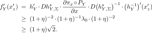 $$ \begin{align*} f_Y'(x^{\prime}_z) ~&=~h^{\prime}_Y \cdot Dh^s_{Y,\Sigma} \cdot \frac{\partial \pi_x\circ P_Y}{\partial x} \cdot D\big( h^s_{Y,\Sigma} \big)^{-1} \cdot \big(h_Y^{-1}\big)'(x^{\prime}_z) \\ ~&\geq~ (1+\eta)^{-2}\cdot (1+\eta)^{-1}\lambda_0 \cdot (1+\eta)^{-2} \\ ~&\geq~(1+\eta)\sqrt{2}. \end{align*} $$
This shows that one-dimensional quotient map
 $f_Y$
satisfies the property of geometric Lorenz attractors.
Since
 $P_Y$
is uniformly contracting in each leaf of
 $\mathcal {F}^s_{Y,\Sigma }$
, the function
 $H_Y$
is contracting along the
 $y'$
-coordinate. The proof of rest properties for
 $H_Y$
is the same with
 $f_Y$
. Thus, we take
 $\mathcal {U}=\mathcal {U}_1\cap \mathcal {U}_2\cap \mathcal {U}_3$
which is a
 $C^2$
-neighborhood of X, and
 $\Lambda _Y$
is a geometric Lorenz attractor for every
 . This completes the proof of Proposition 3.8.
B Appendix: Singular hyperbolic attractors for
$C^1$
-vector fields

For vector fields on a closed smooth manifold M of any dimension in
 $C^1$
-topology, one already has the well-known perturbation techniques such as Hayashi’s connecting lemma [Reference Hayashi35, Reference Wen and Xia73, Reference Wen72] and Bonatti-Crovisier’s chain-connecting lemma [Reference Bonatti and Crovisier12]. Following similar arguments of Section 4 and applying the
 $C^1$
-connecting lemmas, one obtains the same conclusions as in Theorem B and Corollary 1.4 for singular hyperbolic attractors of
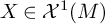 . We sketch the results for completeness. We would like to point out that researches on singular hyperbolic attractors about robust transitivity, hyperbolicity and entropy theory can be found in a series of works [Reference Arbieto, Morales and Santiago5, Reference Crovisier and Yang25, Reference Morales and Pacifico51, Reference Shi, Gan and Wen62, Reference Pacifico, Yang and Jang53]. In particular, a more recent work by S. Crovisier and D. Yang [Reference Crovisier and Yang25] proved that there exists an open dense set
 $\mathcal {U}$
in
 $\mathscr {X}^1(M)$
such that for any
 , any nontrivial singular hyperbolic attractor
 $\Lambda $
is a robustly transitive attractor and
 $\Lambda $
is a homoclinic class in which all periodic orbits are homoclinically related to each other. This ensures that one could follow similar arguments of Section 4 and apply the
 $C^1$
-connecting lemmas to study the space of ergodic measures for singular hyperbolic attractors of
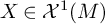 . Similarly as in Theorem B, the space of ergodic measures restricted on singular hyperbolic attractors is path connected for
 $C^1$
-generic vector fields, while on the other hand, for
 $C^1$
-dense vector fields admitting a singular hyperbolic attractor with a co-dimensional two singular hyperbolic splitting, the singular measure is isolated in the space of ergodic measures, which implies in this case that the ergodic measure space is not connected.
Theorem B.1. There exist a residual subset
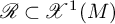 $\mathscr {R}\subset \mathscr {X}^1(M)$
and a dense subset
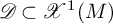 $\mathscr {D}\subset \mathscr {X}^1(M)$
, such that
-
• if
and
$\Lambda $
is a singular hyperbolic attractor of X, then
$\mathcal {M}_{inv}(\Lambda )=\overline {\mathcal {M}_{erg}(\Lambda )}=\overline {\mathcal {M}_{per}(\Lambda )}$
. Moreover, the space
$\mathcal {M}_{erg}(\Lambda )$
is path connected. -
• if
and
$\Lambda $
is a singular hyperbolic attractor of X whose singular hyperbolic splitting
$T_{\Lambda }M=E^{ss}\oplus E^{cu}$
satisfies
$\dim (E^{cu})=2$
, then
$\overline {\mathcal {M}_{per}(\Lambda )}\subsetneqq \overline {\mathcal {M}_{erg}(\Lambda )}\subsetneqq \mathcal {M}_{inv}(\Lambda )$
. Moreover, the space
$\mathcal {M}_{erg}(\Lambda )$
is not connected.
 and



 and





Concerning the residual part of Theorem B.1, similar properties are obtained in [Reference Abdenur, Bonatti and Crovisier1, Theorem 3.5] for isolated nontrivial transitive sets of diffeomorphisms. For vector fields, one has to conquer the difficulties caused by the existence of singularities (i.e., to show that the atomic measure of the singularity can be accumulated by periodic measures inside the singular hyperbolic attractor). This could be achieved by applying Hayashi’s connecting lemma combined with the arguments in Section 4.4. An alternative proof can be found in [Reference Yang and Zhang76, Theorem 3.1], where they proved
 $\mathcal {M}_{inv}(\Lambda )=\overline {\mathcal {M}_{erg}(\Lambda )}=\overline {\mathcal {M}_{per}(\Lambda )}$
for which
 $\Lambda $
is a nontrivial isolated transitive set for
 $C^1$
-generic vector fields.
Similarly as Theorem B, the dense part of Theorem B.1 is a sharp comparison with the residual part. For the dense part, one applies Hayashi’s connecting lemma to make the two branches of the unstable manifolds of the singularity with co-index one lie in the stable manifold of a periodic orbit. Then the arguments follow the dense part in Section 4.4; see also Remark 4.6. A related work by C. Morales [Reference Morales50] proved that every non-transitive sectional-Anosov flow with dense periodic orbits exhibits an invariant measure that cannot be approximated by ergodic ones. The arguments in [Reference Morales50] are quite different from us where the author considered invariant measures that are not supported on a transitive set, while we obtain here isolated ergodic measures inside an attractor.
The following is a corollary of Theorem B.1 which concerns the support and entropy of measures on singular hyperbolic attractors and whose statement is similar to Corollary 1.4.
Corollary B.2. There exists a residual subset
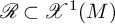 $\mathscr {R}\subset \mathscr {X}^1(M)$
, such that for any
 , if
 $\Lambda $
is a singular hyperbolic attractor of X, then
-
1. there exists a residual subset
$\mathcal {M}_{res}$
in
$\mathcal {M}_{inv}(\Lambda )$
such that every is ergodic with
$\operatorname {Supp}(\mu )=\Lambda $
and
$h_{\mu }=0$
. -
2. there exists a dense subset
$\mathcal {M}_{den}$
in
$\mathcal {M}_{inv}(\Lambda )$
such that every is ergodic with
$h_{\mu }>0$
.


 is ergodic with



 is ergodic with

Remark B.3. Recently, C. Bonatti and A. da Luz [Reference Bonatti and da Luz14] introduced another notion called multisingular hyperbolicity to study more general vector fields with singularities. An interesting question is whether conclusions of Theorem B.1 are true or not for miultisingular hyperbolic chain recurrence classes.
Acknowledgements.
We would like to thank S. Crovisier, S. Gan, G. Liao, C. A. Morales, P. Varandas, L. Wen, D. Yang, J. Yang and J. Zhang for useful suggestions and comments. We are very grateful to the anonymous referee of our paper for her/his valuable comments, which help us a lot to improve the paper. This work was prepared while Y. Shi and X. Wang visited the School of Mathematical Sciences, Fudan University. The two authors would like to thank their hospitality.
Competing interest
The authors have no competing interests to declare.


 closing lemma for Hamiltonian diffeomorphisms of closed surfaces.


 n’a d’orbites périodiques sur un ouvert de surfaces d’énergies.
 des orbites récurrentes de flots hamiltoniens.