

1. Introduction
It has often been advocated that developing countries (DCs) be given more time before being asked to make serious efforts to reduce their greenhouse gas (GHG) emissions. The two underlying reasons for granting them such a delay are: (i) it is industrialized countries (ICs) that are mainly responsible for the current state of the environment, and it would be unfair to constrain DCs' emissions when it is their turn to industrialize; and (ii) compared to other pressing economic issues, such as eradicating extreme poverty, offering essential services to their citizens (education, health care, etc.) and building infrastructure, the environment is seen as a luxury service that DCs cannot really afford in the short term. The historical responsibility of ICs is recognized in international political circles, and was actually accepted in the Kyoto Protocol, where DCs were not asked to reduce their emissions. Further, the argument that reaching a certain level of development has priority over environmental and possibly other social and political concerns appeals to a large community of scholars and decision makers because it corresponds to the successful role-model path followed by the developed countries themselves. The rationale behind this type of thinking is that ‘As incomes rise, the demand for improvements in environmental quality will increase, as will the resources available for investment’ (World Bank, 1992: 39). In fact, this idea of a relationship between welfare (prosperity or development) and environmental concerns has been around for some time, and has been supported by different arguments ranging from the purely materialistic to the post-materialistic and psychological ones. The interested reader may refer to the survey in Martínez-Alier (Reference Martínez-Alier1995) for a complete discussion of the links between economic growth and environmental goods.
Suppose that DCs: (i) need a period of time [0, T] to accomplish a desired level of development, during which they disregard environmental damage, either partially or completely, when making their production decisions; and (ii) fully internalize their environmental externalities after T. Then, the objective of this paper is to address the following research questions:
(1) How do cooperative and non-cooperative emissions strategies compare during this first period [0, T] and in the long run?
(2) Can cooperation between DCs and ICs reduce T?
(3) Under which conditions is cooperation collectively better than non-cooperation during the time interval [0, T?
We believe that these questions are relevant to the negotiations of all environmental agreements involving both types of countries. To answer these questions, we adopt a two-player differential-game model, where player 1 represents developed countries and fully accounts for the environmental damage cost, and player 2 represents DCs and does not consider the environment a top priority during an initial period of time, whose terminal date is endogenous. The choice of a dynamic-game framework to deal with the above questions is quite natural. Indeed, the transboundary nature of pollution emissions calls for a game-theoretic approach to capture the strategic interactions between players. Further, as economic development and environmental concerns are typically long-term problems that cannot be solved overnight, the model must reflect this dynamic feature.
This paper belongs to the significant differential-games literature in environmental economics and, more specifically, to the part dealing with international environmental agreements (IEAs); see, e.g., the recent surveys by Jørgensen et al. (Reference Jørgensen, Martín-Herrán and Zaccour2010) and Long (Reference Long2010). The dynamic IEAs literature can be divided into two streams. In the first stream, the papers characterize and contrast the cooperative and non-cooperative solutions and demonstrate the benefits of cooperation. A pending issue when the game is cooperative is how to allocate the total payoff among the players. Typically, this is done by adopting a cooperative-game solution, e.g., core and Shapley value. The early contributions in this stream are van der Ploeg and de Zeeuw (Reference van der Ploeg and de Zeeuw1992) and Long (Reference Long1992). An impressive list of papers followed, which we will not review but instead refer the reader to the above-cited surveys. The second stream sees the signing of an IEA as a non-cooperative game that ends when a stable coalition is reached, that is, no outsider would like to join the agreement, and no insider would like to leave it. The (static) non-cooperative-game approach to IEAs started two decades ago, and a recurrent result in this literature is that full cooperation is hard to achieve, albeit it is urgently needed to curb emissions and avoid some possible catastrophic events. Recently, we have seen some contributions that include pollution accumulation and membership dynamics in their models; see, e.g., Rubio and Casino (Reference Rubio and Casino2005), Rubio and Ulph (Reference Rubio and Ulph2007), de Zeeuw (Reference de Zeeuw2008), Bahn et al. (Reference Bahn, Breton, Sbragia and Zaccour2009), and Breton et al. (Reference Breton, Sbragia and Zaccour2010).
A main contribution of this paper lies in its different treatment of the two players in terms of their environmental concerns and, consequently, in modeling their damage-cost functions. Indeed, we depart from the often-retained assumption that DCs either fully account for their environmental costs from the outset of the game or never account for them, by supposing that they adopt a gradual-involvement approach in dealing with the environmental externality. By doing this, we hope to capture in a more realistic way the structural asymmetry between the two groups of countries, and not only the asymmetry in parameter values. In some sense, we are extending here the notion of environmental-damage costs to the broader idea of ‘environmental concerns’. Roughly speaking, by environmental concerns we mean any kind of feeling, economic problem and health issue related to emissions or their accumulation. Of course, precisely modeling an environmental concerns function is a highly challenging task at all levels, including the specification of such a function, the measurement of the variables that are supposedly involved and the choice of a functional form. As a first exploratory step in this direction, we suppose that environmental concerns can be represented by a (damage-cost) function whose arguments are the pollution stock (as usual) and accumulated revenues. By letting this function positively depend on revenues until a certain threshold is reached, we are in fact operationalizing in the most parsimonious possible way the World Bank idea quoted above. Another contribution with respect to the dynamic-games literature on pollution control lies in our analysis of emissions strategies and payoffs during the first period of the game. Short-term considerations are generally overlooked in this literature, which has focused only on long-term solutions, that is, on cooperative and non-cooperative steady states in infinite-horizon games.
Our main results can be summarized as follows:
(1) Throughout the game, ICs emit less under cooperation than non-cooperation. The same is observed for DCs but only in the long term, that is, after reaching the threshold level of development. In the shorter term, the result depends on the degree of environmental concern in DCs.
(2) For a large region of the parameter space, cooperation would lead to a longer period of low or total lack of involvement by the DCs in dealing with environmental damage than would non-cooperation. Also, in the short term, cooperation may not create enough dividend to be an attractive mode of play.
(3) It may not be the best option for ICs to press DCs to engage in abatement efforts in the short term.
The rest of the paper is organized as follows: in section 2, we introduce the model, and in section 3, we characterize emissions strategies under cooperative and non-cooperative modes of play, and perform a sensitivity analysis. In section 4, we compare emissions and outcomes under the two regimes and discuss the feasibility of cooperation in the short term. Section 5 briefly concludes.
2. Model
We consider a two-player differential game, where player 1 represents the group of developed countries characterized by high environmental concern levels, and player 2 represents less developed countries for whom environmental issues are not yet at the top of their economic agenda.Footnote 1 Time t is continuous, with t ∈ [0,∞). Denote by e i(t) the emissions of player i at time t. Emissions are a by-product of industrial production activities y i(t), and are given by e i(t) = h i(y i(t)). We suppose that h i(·) is a smooth function that can be inverted, and write  $y_{i}\lpar t\rpar =h_{i}^{-1}\lpar e_{i}\lpar t\rpar \rpar \triangleq f_{i}\lpar e_{i}\lpar t\rpar \rpar $; that is, we can express production (or revenue) as a function of emission levels. We make the standard assumption that f i(e i) is concave and increasing.
Denote by S(t) the stock of pollution, whose evolution is described by the following differential equation:
 $$\dot{S}\lpar t\rpar = \mu\lpar e_1\lpar t\rpar + e_2\lpar t\rpar \rpar - \delta S\lpar t\rpar \comma \; \quad S\lpar 0\rpar = S_0\comma \; $$
where μ is a positive scaling parameter, δ is the positive natural absorption rate of pollution, and S 0 is the initial given pollution stock.
2.1. Environmental cost
In the transboundary pollution literature, (see Jørgensen et al., Reference Jørgensen, Martín-Herrán and Zaccour2010 for a survey), the usual assumption is that, from the outset, all players account for the full environmental damage cost when making their production decisions. The damage cost of player i, denoted by D i(S), is assumed to be an increasing convex function of the stock of pollution. We retain this assumption for player 1, the representative of developed countries that can afford to fully internalize the environmental cost. For player 2, we assume that this internalization of the environmental cost is gradual, and will become complete only when a threshold level of economic development has been achieved. To reflect this, the damage cost is modeled as a function of the pollution stock and of the level of development during a first period of time, and a function of only the pollution stock after that period. Adequately measuring a country's development level is a difficult task and requires the use of a long list of variables, e.g., available infrastructure, consumption per capita, life expectancy, etc. To keep the model as parsimonious as possible without, however, losing much qualitative insight into the problem we are dealing with, we avoid taking this route and simply assume that the level of development can be well approximated by cumulative revenues. Note that we could add environmental awareness (or information acquisition) as a determinant of environmental concerns, but refrain from doing so, assuming that cumulative revenues and awareness are highly correlated variables, and that therefore there is no need to retain both of them. In fact, our simple reasoning is consistent with Shafik and Bandyopadhyay (Reference Shafik and Bandyopadhyay1992) who found, using data from 149 countries for the period 1960–1990, that ‘income has the most consistently significant effect on all indicators of environmental quality’.
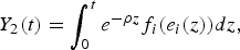
We assume that both players discount future gain using the same constant rate of time preference ρ > 0. Denote by Y 2(t) the cumulative discounted revenues of player 2 by time t, which is given by
 $$Y_2\lpar t\rpar =\int_0^{t}e^{-\rho z}f_{i}\lpar e_{i}\lpar z\rpar \rpar dz\comma \;$$
and by  $\bar{Y}_2$ the threshold value of cumulative revenues before this player starts to fully account for the environmental damage. The damage-cost function of player 2 is then specified as
 $$D_2\lpar S\lpar t\rpar \comma \; Y_2\lpar t\rpar \rpar = \left\{\matrix{d_2\lpar S\lpar t\rpar \comma \; Y_2\lpar t\rpar \rpar \comma \; \hfill & \forall Y_2\lpar t\rpar \lt \bar{Y}_2\comma \; \hfill \cr D_2\lpar S\lpar t\rpar \rpar \comma \; \hfill & \forall Y_2\lpar t\rpar \geq \bar{Y}_2\comma \; \hfill} \right.$$
with
 $${\partial D_2\lpar S\comma \; Y_2\rpar \over \partial S} \gt 0\comma \; \quad {\partial^2D_2\lpar S\comma \; Y_2\rpar \over \partial S^2}\geq 0\comma \; \quad {\partial D_2\lpar S\comma \; Y_2\rpar \over \partial Y_2}\geq 0.$$
Finally, we note that there is a common element between our approach and the well-known environmental Kuznets curve (EKC) approach, namely, the existence of a link between income and environmental quality.
2.2. Payoffs and functional forms
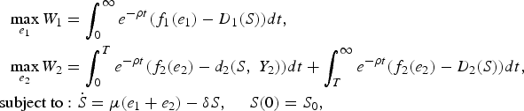
We will henceforth skip the time argument when no ambiguity may arise. We suppose that each player's objective is to maximize his discounted stream of welfare, given by the difference between production revenues and the damage cost. The optimization problems of the two players are then as follows:
 $$\eqalign{\max_{e_1}W_1 &=\int_0^{\infty}e^{-\rho t}\lpar f_1\lpar e_1\rpar - D_1\lpar S\rpar \rpar dt\comma \; \cr \max_{e_2}W_2 &=\int_0^{T}e^{-\rho t}\lpar f_2\lpar e_2\rpar -d_2\lpar S\comma \; Y_2\rpar \rpar dt + \int_{T}^{\infty}e^{-\rho t}\lpar f_2\lpar e_2\rpar -D_2\lpar S\rpar \rpar dt\comma \; \cr \hbox{subject to} &\colon \dot{S} = \mu\lpar e_1 + e_2\rpar - \delta S\comma \; \quad S\lpar 0\rpar = S_0\comma \; }$$
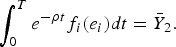
where T is the date satisfying the following equality:
 $$\int_0^{T}e^{-\rho t}f_{i}\lpar e_{i}\rpar dt = \bar{Y}_2. $$
Remark 1
Since there is a one-to-one correspondence between T and  $\bar{Y}_2$, we can express, with a slight abuse of notation, the damage cost of player 2 as a function of time instead of writing it as a function of cumulative revenues, that is,
 $$D_2\lpar S\lpar t\rpar \comma \; t\rpar = \left\{\matrix{d_2\lpar S\lpar t\rpar \comma \; t\rpar \comma \; \hfill & \forall t \lt T\comma \; \hfill \cr D_2\lpar S\lpar t\rpar \rpar \comma \; \hfill & \forall t\geq T.\hfill} \right.$$
To illustrate the type of insight that can be derived using our model, from now on, we adopt the following functional forms:
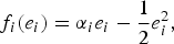 $$f_{i}\lpar e_{i}\rpar = \alpha_{i}e_{i} - {1 \over 2} e_{i}^2\comma \; $$
 $$D_1\lpar S\rpar = \beta_1S\comma \; $$
 $$D_2\lpar S\lpar t\rpar \comma \; Y_2\lpar t\rpar \rpar = \left\{\matrix{\displaystyle{t \over T} \gamma \beta_2S\comma \; \hfill & \forall Y_2\lpar t\rpar \lt \bar{Y}_2\comma \; \hfill \cr \beta_2S\comma \; \hfill & \forall Y_2\lpar t\rpar \geq\bar{Y}_2. \hfill}\right.$$
In the revenue function in (3), the parameter αi, i = 1, 2, is strictly positive, and the implicit assumption is that f i(e i) is strictly positive for all possible actual pollution values. This quadratic form is common in the literature; see, e.g., Smala Fanokoa et al. (Reference Smala Fanokoa, Telahigue and Zaccour2011), Dockner and Long (Reference Dockner and Long1993), Breton et al. (Reference Breton, Zaccour and Zahaf2005) and Rubio and Casino (Reference Rubio and Casino2005). The damage-cost functions of both players are assumed linear in the stock, with parameters β1 and β2 being strictly positive. Admittedly, the linearity assumption of the damage cost is a considerable simplification. However, we expect the impact of this choice on the results to be quantitative and not qualitative. We note that our linearity assumption is not uncommon in the modeling literature (see, e.g., Hoel and Schneider, Reference Hoel and Schneider1997; Breton et al., Reference Breton, Sbragia and Zaccour2010), and is also supported in some empirical contributions (see, e.g., Labriet and Loulou, Reference Labriet and Loulou2003). This being said, it would be of interest to extend the analysis to a non-linear damage cost in future works. Further, we suppose that γ ∈ {0,1}. A value γ = 0 means that player 2 completely ignores the environmental damage before reaching T. This is meant to represent an extreme case where this player is experiencing harsh development problems, and is not willing to account for environmental externalities when making his production decisions, until he reaches the sought-for threshold of cumulative wealth  $\bar{Y}_2$. This is somehow in the spirit of the Kyoto Protocol, where DCs were not requested to reduce their emissions. The case γ = 1 corresponds to a gradual internalization of the damage cost. We now contrast the results of the two cases.
2.3. Solution concepts
We will characterize and compare the cooperative and non-cooperative solutions to the two-player differential game introduced above. We suppose that the information structure is feedback; that is, the pollution strategy of each player is a function of the state variable (pollution stock). The cooperative game corresponds to the scenario where the two players sign an IEA aiming at controlling pollution. In such a context, the optimal pollution levels are obtained by jointly maximizing the welfare of the two players. The results will be superscripted by C (for cooperation). In the absence of an agreement, the game is played non-cooperatively, and the two players seek a Nash equilibrium. The results will be superscripted by N (for Nash equilibrium).
Because of the assumption made about the damage-cost function of player 2, the determination of the two solutions is much more complicated than in the case where the damage cost does not vary over time. Indeed, both cooperative and non-cooperative solutions will depend on the date at which player 2 becomes fully vulnerable to the environmental damage. To handle this, we proceed backward; that is, we assume that we know T j, j = C, N, and solve the infinite-horizon problem defined on [T j,∞). Next, we deal with the first-period problem defined on [0, T j], using the second-period value functions as salvage values in the overall optimization problem defined on [0, ∞). At this stage, we have the information to compute T j and S(T j), which at the beginning were assumed given, by inserting the optimal strategies into (2). Note that the date T j will not only depend on the mode of play, but also on the value of the parameter γ. To reflect this, we will write T j when a result holds for both values of γ, and subscript T j with γ when the result holds for a specific value of γ, that is, T γj, with T 0j and T 1j corresponding to γ = 0, 1, respectively.
3. Results
3.1. Non-cooperative and cooperative emissions
To save on notation, define by
 $$\eqalign{F\lpar t\semicolon \; T^{N}\rpar &= {1+t\lpar \rho+\delta\rpar -e^{\lpar \rho+\delta\rpar \lpar t-T^{N}\rpar } \over \lpar \rho+\delta\rpar T^N}\comma \; \quad G\lpar t\semicolon \; T^{N}\rpar = 1 - e^{\lpar \rho + \delta\rpar \lpar t - T^N\rpar }\comma \; \cr F\lpar t\semicolon \; T^{C}\rpar &= {1 + t\lpar \rho + \delta\rpar - e^{\lpar \rho+\delta\rpar \lpar t - T^C\rpar } \over \lpar \rho+\delta\rpar T^C}\comma \; \quad G\lpar t\semicolon \; T^{C}\rpar = 1 - e^{\lpar \rho + \delta\rpar \lpar t - T^C\rpar }.}$$
We first characterize the feedback-Nash equilibrium, and next determine the cooperative solution.
Proposition 1
Assuming an interior solution, the feedback-Nash equilibrium emissions are given by
 $$\eqalign{e_1^{N}\lpar t\rpar &= \alpha_1 - {\mu\beta_1 \over \rho + \delta}\comma \; \quad \forall t\in\lsqb 0\comma \; \infty\rpar \comma \; \cr e_2^{N}\lpar t\rpar &= \left\{\matrix{\alpha_2 - {\mu\beta_2 \over \lpar \rho + \delta\rpar } \lpar \gamma F\lpar t\semicolon \; T^N\rpar + e^{\lpar \rho+\delta\rpar \lpar t - T^N\rpar } \lpar 1 - \gamma\rpar \rpar \comma \; \hfill & \hbox{for }t\in\lsqb 0\comma \; T^N\rsqb \comma \; \cr \alpha_2 - {\mu\beta_2 \over \rho + \delta}\comma \; \hfill & \hbox{for }t\in\lsqb T^N\comma \; \infty\rpar \comma \; }\right.}$$
where T Nis the solution to the equation
 $$\int_0^{T^{N}}\left(\alpha_2e_2^{N} - {1 \over 2} \lpar e_2^N\rpar ^2 \right)e^{-\rho t}dt = \bar{Y}_2. $$
Proof See online Appendix 1 available at http://journals.cambridge.org/EDE.
The results in the above proposition call for four observations. First, the equilibrium strategies are independent of the state variable (pollution stock). This is a by-product of the linear-state structure of the adopted differential game. Second, the strategy of player 1 is the same before and after T N, which is expected since this player is fully vulnerable to the environmental damage from the beginning of the game. Third, the given expression for e 2N is valid for any γ ≥ 0. Specializing the results in each value of γ, we get the following emissions trajectory for player 2 for t≤ T γN:
 $$e_2^{N}\lpar t\semicolon \; \gamma\rpar = \left\{\matrix{\alpha _2 - {\mu \over \lpar \rho +\delta\rpar ^2} {\beta _2 \over T_1^N} \lpar 1 + t\lpar \rho + \delta \rpar -e^{\lpar \rho +\delta\rpar \lpar t-T_1^{N}\rpar }\rpar \comma \; \hfill & \hbox{for }\gamma =1\comma \; \cr \alpha _2 - {\mu \beta _2 \over \lpar \rho +\delta\rpar } \lpar e^{\lpar \rho +\delta\rpar \lpar t-T_0^{N}\rpar }\rpar \comma \; \hfill & \hbox{for }\gamma = 0.} \right.$$
The sign of the difference
 $$\eqalign{e_2^{N}\lpar t\semicolon \; 0\rpar -e_2^{N}\lpar t\semicolon \; 1\rpar &= {\beta _2\mu \over T_1^N\lpar \rho +\delta\rpar ^2} \lpar 1-e^{\lpar t-T_1^{N}\rpar \lpar \rho +\delta \rpar } \cr &\quad + \lpar \rho +\delta\rpar \lpar t - T_1^{N}e^{\lpar t-T_0^{N}\rpar \lpar \rho +\delta\rpar }\rpar \rpar \comma \; } $$
cannot be unambiguously determined, as it depends on the parameter values, and on the dates T 0N and T 1N. We will come back to this later. Fourth, the emissions level of player 2 are monotonically decreasing over time during the time interval [0, T N], and reach their lowest value at T N, that is, when this player becomes fully vulnerable to the environmental damage. Indeed, computing the derivative of e 2N with respect to time, we get
 $$\eqalign{\dot{e}_2^{N}\lpar t\rpar & = - {\mu \over \lpar \rho +\delta \rpar } {\beta _2 \over T^N} \lpar \gamma \lpar 1 - e^{\lpar \rho +\delta\rpar \lpar t-T^{N}\rpar }\rpar \cr &\quad +e^{\lpar \rho +\delta \rpar \lpar t-T^{N}\rpar } \lpar T^N\lpar \rho +\delta \rpar \lpar 1-\gamma \rpar \rpar \rpar \lt 0.}$$
Note that t = T γN, γ∈ {0,1}; the emissions are given by
 $$e_2^{N}\lpar T_{\gamma}^{N}\semicolon \; \gamma\rpar = \alpha_2 - {\mu \beta_2 \over \lpar \rho +\delta\rpar }\comma \;$$
that is, the same value as the one computed for the long run, i.e., after T N.
To solve for the dynamics in (1), that is, to determine the equilibrium pollution-stock trajectory and the steady-state value, we design the following algorithm and use it in the next section:
Step 1
Compute T γN for γ ∈ {0,1} using (2), that is,
 $$\eqalign{&\int_0^{T}e^{-\rho t}f_2\lpar e_2^{N}\lpar t\semicolon \; \gamma\rpar \rpar dt \cr &\quad = \left\{\matrix{\int_0^{T}e^{-\rho t}\left(\alpha_2e_2^{N}\lpar t\semicolon \; 1\rpar - {1 \over 2} \lpar e_2^{N}\lpar t\semicolon \; 1\rpar \rpar ^2\right)dt = \bar{Y}_2\comma \; & \gamma=1\comma \; \cr \int_0^{T_0}e^{-\rho t}\left(\alpha_2e_2^{N}\lpar t\semicolon \; 0\rpar -{1 \over 2}\lpar e_2^{N}\lpar t\semicolon \; 0\rpar \rpar ^2\right)dt = \bar{Y}_2\comma \; & \gamma = 0.}\right. }$$
Step 2
For t∈ [0,T γN], γ ∈ {0,1}, solve the differential equation
 $$\dot{S} = \left\{\matrix{\mu\lpar e_1^{N}\lpar t\rpar + e_2^{N}\lpar t\semicolon \; 1\rpar \rpar - \delta S\comma \; \quad S\lpar 0\rpar = S_0\comma \; & \gamma = 1\comma \; \cr \mu\lpar e_1^{N}\lpar t\rpar + e_2^{N}\lpar t\semicolon \; 0\rpar \rpar - \delta S\comma \; \quad S\lpar 0\rpar = S_0\comma \; & \gamma=0.} \right.$$
Let  $S_{T_{\gamma}^N}$ be the value of the pollution stock at T γN, γ∈ {0,1}.
Step 3
For t∈ [T γN, ∞), γ∈ {0,1}, solve the differential equation
 $$\dot{S} = \left\{\matrix{\mu\lpar \alpha_1+\alpha_2 - \displaystyle{\mu \over \rho+\delta}\lpar \beta_1+\beta_2\rpar \rpar -\delta S\comma \; &S\lpar T_1^{N}\rpar = S_{T_1^{N}}\comma \; &\gamma=1\comma \; \cr \mu\lpar \alpha_1 + \alpha_2 - \displaystyle{\mu \over \rho + \delta}\lpar \beta_1 + \beta_2\rpar \rpar - \delta S\comma \; &S\lpar T_0^{N}\rpar = S_{T_0^N}\comma \; &\gamma=0.}\right.$$
The above equation has as its solution
 $$S^{N}\lpar t\rpar = \left\{\matrix{\matrix{\displaystyle{1 \over \delta}\mu\lpar \alpha_1 + \alpha_2 - {\mu \over \rho + \delta} \lpar \beta_1 + \beta_2\rpar \rpar \lpar 1 - e^{\delta\lpar T_1^{N}-t\rpar }\rpar \cr +\, e^{\delta\lpar T_1^{N}-t\rpar }S_{T_1^{N}}\comma \; } & \gamma = 1\comma \; \cr \matrix{\displaystyle{1 \over \delta}\mu\lpar \alpha_1 + \alpha_2 - {\mu \over \rho+\delta} \lpar \beta_1 + \beta_2\rpar \rpar \lpar 1 - e^{\delta\lpar T_0^{N}-t\rpar }\rpar \cr +\, e^{\delta\lpar T_0^{N}-t\rpar }S_{T_0^{N}}\comma \; } & \gamma = 0.} \right.$$
The steady-state value is independent of γ, and is given by
 $$S_{ss}^{N} = \lim_{t\rightarrow\infty}S^{N}\lpar t\rpar = {\mu \over \delta} \left(\alpha_1 + \alpha_2 - {\mu \over \rho + \delta} \lpar \beta_1 + \beta_2\rpar \right).$$
The following proposition characterizes cooperative emissions strategies.
Proposition 2
Assuming an interior solution, the optimal emissions of player i, i = 1, 2, are given by
 $$e_{i}^{C}\lpar t\rpar = \left\{\matrix{\matrix{\alpha_{i} - \displaystyle{\mu\beta_1 \over \rho+\delta} - \displaystyle{\mu\beta_2 \over \lpar \rho+\delta\rpar } \lpar \gamma F\lpar t\semicolon \; T^{C}\rpar \cr {+}\, e^{\lpar \rho+\delta\rpar \lpar t-T^{C}\rpar } \lpar 1 - \gamma\rpar \rpar \comma \; } & \hbox{for }t\in\lsqb 0\comma \; T^{C}\rsqb \comma \; \cr \alpha_{i} - \mu \displaystyle{\beta_1 + \beta_2 \over \rho + \delta}\comma \; \hfill & \hbox{for } t\in\lsqb T^{C}\comma \; \infty\rpar \comma \; }\right.$$
where T Cis the solution to the equation
 $$\int_0^{T^C} \left(\alpha_2e_2^{C} - {1 \over 2} \lpar e_2^C\rpar ^2 \right)e^{-\rho t}dt = \bar{Y}_2.$$
Proof: See online Appendix 2.
The two main differences with the non-cooperative case are: (i) player i now accounts for player j's marginal damage cost βj, which is a standard result in cooperative environmental games; and (ii) player 1's emissions are now a function of time during the interval [0, T C], that is, until the date at which player 2 reaches his full environmental vulnerability. Further, we note that both players decrease their emissions by the same rate over time during the interval [0, T C]. Indeed, computing the derivative of e iC(t) with respect to time yields
 $$\eqalign{\dot{e}_{i}^{C}\lpar t\rpar & = - {\mu\beta_2 \over T^{C}\lpar \rho+\delta\rpar } \lpar \gamma\lpar 1 - e^{\lpar \rho + \delta\rpar \lpar t - T^{C}\rpar }\rpar \cr &\quad +e^{\lpar \rho + \delta\rpar \lpar t - T^{C}\rpar }\lpar T^{C}\lpar \delta + \rho\rpar \lpar 1 - \gamma\rpar \rpar \rpar \lt 0\comma \; \quad i = 1\comma \; 2.}$$
As in the non-cooperative case, T C depends on γ, and will be denoted by T γC. To compute this date and the optimal pollution-stock trajectory, we follow the same algorithm as in the non-cooperative scenario. It can easily be shown that the steady state here is given by
 $$S_{ss}^{C} = {\mu \over \delta} \left(\alpha_1 + \alpha_2 - {2\mu \over \rho + \delta} \lpar \beta_1 + \beta_2\rpar \right).$$
Remark 2
We assume that the parameter values are such that all equilibrium and optimal emissions and steady-state pollution values are strictly positive. In particular, this requires imposing the following condition:
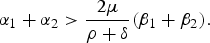 $$\alpha_1 + \alpha_2 \gt {2\mu \over \rho + \delta} \lpar \beta_1 + \beta_2\rpar .$$
3.2. Comparative statics
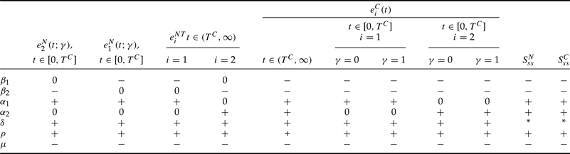
Table 1 summarizes the effect of the model's parameters on the players' strategies for the whole time horizon, and on the steady-state pollution stock under cooperative and non-cooperative modes of play. In the non-cooperative scenario, a higher marginal cost βi leads to lower emissions e iN, i = 1, 2, and has no effect on e jN, j ≠ i. Under cooperation, an increase in either marginal damage cost has a negative effect on both players' emissions. This is because each member of the coalition accounts for the damage to all players when determining his pollution strategy. The impact of varying αi is, as expected, positive on the emissions of player i. A higher discount rate, i.e., attaching less value to future damages, encourages players to increase their today's revenues by emitting more, and consequently we obtain a higher steady-state pollution. Further, the impact of varying the natural absorption on the steady state of the pollution stock is a priori ambiguous. Indeed, increasing δ is synonymous with an improvement in abatement technology and, hence, with a higher reduction in the existing stock. On the other hand, a higher δ is an incentive to increase today's emissions. However, under condition (8), we obtain that the net impact of increasing δ on the non-cooperative steady state is negative. The same holds true for the cooperative steady state for sufficiently low δ.
Parameter effects on emissions and steady-state stock, cooperative and non-cooperative cases.

Notes: Most of the results in table 1 are straightforward. To save space, we do not report the derivatives. Only the results regarding the variation of the steady state with respect to δ merit some detail. The derivatives are given by
 $$\eqalign{{\partial S_{ss}^{C} \over \partial\delta} &= - {\mu\lpar \lpar \alpha_1+\alpha_2\rpar \lpar \delta+\rho\rpar ^2-2\mu\lpar \beta_1+\beta_2\rpar \lpar 2\delta+\rho\rpar \rpar \over \delta^2\lpar \delta+\rho\rpar ^2}\comma \; \cr {\partial S_{ss}^{N} \over \partial\delta} &= -{\mu\lpar \lpar \alpha_1+\alpha_2\rpar \lpar \delta+\rho\rpar ^2-\mu\lpar \beta_1+ \beta_2\rpar \lpar 2\delta+\rho\rpar \rpar \over \delta^2\lpar \delta+\rho\rpar ^2}.}$$
Clearly, we have  ${\partial S_{ss}^{N} \over \partial\delta} \lt 0\Leftrightarrow\alpha_1 + \alpha_2 \gt \mu\lpar \beta_1 + \beta_2\rpar {\lpar 2\delta+\rho\rpar \over \lpar \delta+\rho\rpar ^2}\comma \; $ which always holds true under condition (8). For
 ${\partial S_{ss}^{C} \over \partial\delta}$ to be negative, we need
 $\alpha_1+ \alpha_2 \gt 2\mu\lpar \beta_1 + \beta_2\rpar {\lpar 2\delta+\rho\rpar \over \lpar \delta+\rho\rpar ^2}\comma \; $ which is satisfied if δ is sufficiently small.
4. Comparison
In this section, we first compare cooperative and non-cooperative emissions, and then the corresponding outcomes.
4.1. Comparison of emissions
The next two propositions compare the non-cooperative and cooperative emissions of player 1 and 2, respectively.
Proposition 3
Player 1 emits more in the non-cooperative game than under cooperation at all instants of time, that is,
 $$e_1^{N}\lpar t\rpar \gt e_1^C \lpar t\rpar \comma \; \quad \forall t\in\lsqb 0\comma \; \infty\rpar .$$
Proof: We need to show the result for two time intervals, namely, [0, T C] and [T C,∞). For t ∈ [0, T C], the difference in emissions is given by
 $$\eqalign{e_1^{N}\lpar t\rpar -e_1^{C}\lpar t\rpar & = {\mu\beta_2 \over T^C \lpar \rho + \delta\rpar ^2} \lpar \gamma\lpar 1 + t\lpar \rho + \delta\rpar - e^{\lpar \rho + \delta\rpar \lpar t - T^C\rpar }\rpar \cr &\quad +e^{\lpar \rho + \delta\rpar \lpar t - T^C\rpar } \lpar T^C \lpar \delta + \rho\rpar \lpar 1 - \gamma\rpar \rpar \rpar \comma \; }$$
which is clearly positive. For t∈ [T C,∞), we have
 $$e_1^{N}\lpar t\rpar - e_1^{C}\lpar t\rpar = {\mu\beta_2 \over \rho + \delta} \gt 0.$$
Proposition 4
Player 2's cooperative and non-cooperative emissions compare as follows:
(1) For all t≥ max {T N,T C}, we have
(9) $$e_2^{N}\lpar t\rpar - e_2^{C}\lpar t\rpar = {\mu\beta_1 \over \rho + \delta} \gt 0. $$
(2) For all t∈ [min{T N,T C}, max {T N,T C},
(a) If T N < T C, then ∀ t∈ [T N,T C], we have
$$\eqalign{&e_2^{N}\lpar t\rpar - e_2^{C}\lpar t\rpar \cr &\quad = \left\{\matrix{\matrix{\displaystyle{\mu \over \rho + \delta} \lsqb \beta_1 - \beta_2\lpar 1 - F\lpar t\semicolon \; T^{C}\rpar \rpar \rsqb \comma \; \cr \gt \, 0 \Leftrightarrow \displaystyle{\beta_1 \over \beta_2} \gt 1 - F\lpar t\semicolon \; T^{C}\rpar \comma \; } & \gamma = 1\comma \; \cr \displaystyle{\mu \over \rho + \delta} \lsqb \beta_1 - \beta_2G \lpar t\semicolon \; T^C\rpar \rsqb \gt 0 \Leftrightarrow {\beta_1 \over \beta_2} \gt G\lpar t\semicolon \; T^{C}\rpar \comma \; &\gamma = 0.}\right.}$$(b) If T N > T C, then for all t∈ [T C,T N], we have
$$e_2^{N}\lpar t\rpar - e_2^{C}\lpar t\rpar = \left\{\matrix{\displaystyle{\mu \over \rho + \delta} \lsqb \beta_1 + \beta_2\lpar 1 - F\lpar t\semicolon \; T^{N}\rpar \rpar \rsqb \gt 0\comma \; & \gamma = 1\comma \; \cr \displaystyle{\mu \over \rho + \delta}\lsqb \beta_1 + \beta_2G\lpar t\semicolon \; T^{N}\rpar \rsqb \gt 0\comma \; & \gamma = 0.}\right.$$(3) For all t∈ [0, min {T N,T C}, we have
$$\eqalign{&e_2^{N}\lpar t\rpar - e_2^{C}\lpar t\rpar \cr &\quad =\left\{\matrix{\matrix{\displaystyle{\mu \over \rho + \delta} \lsqb \beta_1 + \beta_2 \lpar F\lpar t\semicolon \; T^{C}\rpar - F\lpar t\semicolon \; T^{N}\rpar \rpar \rsqb \gt 0\Leftrightarrow \cr \displaystyle{\beta_1 \over \beta_2} \gt F\lpar t\semicolon \; T^N\rpar - F\lpar t\semicolon \; T^{C}\rpar \comma \; } & \gamma = 1\comma \; \cr \matrix{\displaystyle{\mu \over \rho + \delta} \lsqb \beta_1 + \beta_2\lpar e^{\lpar \rho + \delta\rpar \lpar t - T^{C}\rpar } - e^{\lpar \rho + \delta\rpar \lpar t - T^{N}\rpar }\rpar \rsqb \gt 0\Leftrightarrow \cr \displaystyle{\beta_1 \over \beta_2} \gt e^{\lpar \rho + \delta\rpar \lpar t - T^{N}\rpar } - e^{\lpar \rho + \delta\rpar \lpar t - T^C\rpar }\comma \; } & \gamma = 0.} \right.}$$



Proof Straightforward algebraic manipulations lead to the results.
Based on the results in the above two propositions, the answer to our first research question is as follows:
(1) In the long run, cooperation leads to lower emissions. This result is fully in line with the related literature. Indeed, when each player accounts for the damage cost of all players, he emits less. Consequently, the steady-state value of the pollution stock in the non-cooperative game is higher than in its cooperative counterpart, with the difference being given by
$$S_{ss}^{N}-S_{ss}^{C} = {\mu^2\lpar \beta_1+\beta_2\rpar \over \delta\lpar \rho + \delta\rpar } \gt 0.$$(2) In the short run, there is no definite conclusion regarding player 2's emissions. The relationship between cooperative and non-cooperative emissions depends, in a complex way, on the parameter values. The message here is that cooperation may not necessarily lead to a reduction in emissions by all parties. However, under some conditions stated in the corollary below, we obtain that player 2's non-cooperative emissions are greater than his cooperative emissions for all instants of time, that is, including in the short run.

Corollary 1
Suppose γ = 0. If β1 > β2, then e 2N(t) − e 2C(t) > 0,∀ t∈ [0,∞).
Proof: For t≥ max{T N,T C6}, we have
 $$e_2^{N}\lpar t\rpar - e_2^{C}\lpar t\rpar = {\mu\beta_1 \over \rho + \delta} \gt 0.$$
For all t∈ [min {T N,T C},max{T N,T C}],
• If T N < T C, then
$\forall t\in\lsqb T^{N}\comma \; T^{C}\rsqb $, we have
which is positive as 0 < G(t;T C) < 1.$$e_2^{N}\lpar t\rpar - e_2^{C}\lpar t\rpar = {\mu \over \rho + \delta}\lsqb \beta_1 - \beta_2G\lpar t\semicolon \; T^{C}\rpar \rsqb \comma \;$$• If T N > T C, then for all t∈ [T C,T N], we have
$$e_2^{N}\lpar t\rpar -e_2^{C}\lpar t\rpar = {\mu \over \rho + \delta}\lsqb \beta_1 + \beta_2G\lpar t\semicolon \; T^{N}\rpar \rsqb \gt 0.$$



For all  $t\in\lsqb 0\comma \; \min\lcub T^{N}\comma \; T^{C}\rcub \rsqb \comma \; $ we have
 $$e_2^{N}\lpar t\rpar -e_2^{C}\lpar t\rpar = {\mu \over \rho + \delta}\lsqb \beta_1 + \beta_2\lpar e^{\lpar \rho + \delta\rpar \lpar t - T^{C}\rpar } - e^{\lpar \rho+\delta\rpar \lpar t-T^{N}\rpar }\rpar \rsqb \comma \;$$
which is positive because  $0<e^{\lpar \rho+\delta\rpar \lpar t-T^{C}\rpar }<1$ and
 $0\leq e^{\lpar \rho+\delta\rpar \lpar t-T^{N}\rpar }\leq1.$
Note that the condition β1 > β2 is sufficient and not necessary. Whether it is fulfilled or not is an empirical matter beyond the scope of this paper. At first glance, we may think that this condition does not hold true because DCs are probably less prepared than richer ICs to cope with the environmental damage, including that induced by rising ocean level, floods, and other extreme events.
4.2. Comparison of threshold dates and outcomes
Our second and third research questions refer to comparative outcomes, in terms of the value of γ and the mode of play (cooperative versus non-cooperative), as well as to threshold dates T N and T C. Unfortunately, almost all these comparisons cannot be carried out analytically and we need to resort to numerical simulations.
Our model has nine parameters, namely, αi, βi, μ, ρ,  $\delta\comma \; \bar{Y}_2$ and S 0, i = 1, 2. To start with, we rely on the literature to select values for some of the parameters. Based on Nordhaus (Reference Nordhaus1993), we retain μ = 0.64 and δ = 0.0083 as reference values, and let these parameters vary in the following intervals: μ ∈ [0.5, 1] and δ∈ [0.001,0.01]. Further, we assume that ρ∈ [0.02, 0.2], which is a sufficiently large interval. The calibration of the remaining parameters, that is,
 $\alpha_{i}\comma \; \beta_{i}\comma \; \bar{Y}_2$ and S 0, i = 1, 2, must be made subject to the satisfaction of non-negativity for revenues, emissions and pollution-stock values at each instant of time. The following choice for αi,βi,i = 1,2, leads to a large feasible region: αi∈ [0.5,1] and βi ∈ [0.001,0.01] (note that for some combinations of parameter values, we may still get a negative value for the emissions). The values of
 $\bar{Y}_2$ and S 0 are selected in each simulation conditionally to the choice of the other parameters and satisfaction of the non-negativity constraints. To summarize, we retain upper bounds for αi and μ that are twice their lower-bound values, and upper bounds for δ, ρ and βi that are 10-fold their respective lower bounds. With such a large parameter space, we believe that our numerical results are sufficiently robust to allow for some general qualitative conclusions.
Our second research question was ‘Can cooperation between DCs and ICs shorten the first period of low or full absence of involvement by the DCs in dealing with environmental externalities?’. The answer is clear-cut in the case of γ = 0. Indeed, we prove in the proposition below that cooperation delays the point in time at which DCs would start to fully internalize the environmental externality.
Proposition 5
If γ = 0, then T N < T C.
Proof See online Appendix 3.
Unfortunately, we were not able to analytically prove a similar result for γ = 1. The expressions involved are highly non-linear in T N and T C. We ran a large number of simulations in which we visited the whole numerical grid (in a discrete sense), and obtained either an infeasible result (i.e., negative emissions) or that T N < T C. Based on this, we also conclude that when DCs partially account for the negative environmental externality, they will reach the threshold point in terms of cumulative revenues  $\bar{Y}_2$ earlier when the game is non-cooperative than when it is cooperative. As this result is numerical, we state it as a claim rather than as a proposition.
Claim 1
If γ = 1, then T N < T C.
The intuition is that as DCs are more motivated by revenue in the short run, they will produce and consequently emit more (at lower cost) under the non-cooperative setup, and consequently achieve the threshold sooner.
Moving to the comparison of outcomes, we start by looking at the impact of γ on non-cooperative payoffs (we account for cooperation later on). Recall that, during the first period, DCs face a damage cost given by  ${t \over T}\gamma \beta_2S$, with γ∈ {0,1}. We recall that the damage cost is interpreted in a broad sense and includes abatement efforts. If the total payoff when γ = 1 is larger than the total payoff when γ = 0, then an argument can be made to press DCs to start dealing with environmental externalities from the outset.
Let Δγ be the difference between total non-cooperative payoffs when γ = 0 and γ = 1, i.e.,
 $$\Delta_{\gamma}=\sum_{i=1}^2\lpar W_{i}^{N}\lpar \gamma=0\rpar -W_{i}^{N}\lpar \gamma=1\rpar \rpar .$$
Our numerical results are summarized in figures 1–3. These figures show that  $\Delta _{\gamma }$ is positive for the following combinations of parameter values: (i) the discount rate and the marginal damage cost of player 1 are large, while the marginal damage cost of player 2 is small (see figure 1, left panel; figure 2); (ii) the discount rate and αi, i = 1, 2, are large enough (figure 1, right panel); (iii) the scaling parameter μ is large enough and the absorption rate δ is small enough (figure 2, right panel); and finally (iv) for a large enough initial pollution stock (figure 3, right panel). A first conclusion here is that we can get
 $\Delta _{\gamma }>0$ for very different reasons, e.g., high asymmetry in marginal damage cost, high revenues from production (emissions), and fast accumulation of pollution (high initial stock, or large μ and small δ).
The region with Δγ > 0. Left panel effects of β1, β2 and ρ, right panel effects of α1, α2 and ρ, when δ = 0.003, μ = 0.8, S 0 = 5, and 2 < Ŷ < 8 (depending on different parameter values on the figure)
The region with Δγ > 0. Left panel effects of β1, β2, right panel effects of μ and δ, when ρ = 0.04, δ = 0.003, μ = 0.8, S 0 = 5, 2 < Ŷ < 8 (depending on different parameter values on the figure)
The region with Δγ > 0. Effect of initial state, S 0, α1 and α2, when ρ = 0.04, δ = 0.003, μ = 0.8, S 0 = 5, 2 < Ŷ < 8
In an attempt to find a commonality in the above combinations, we again look at the emissions for the two different values of γ, that is, e 2N(t;0) and e 2N(t;1). (The difference is given in (7), with T 0N and T 1N yet to be computed.) Although it was not possible to sign the difference e 2N(t;0) − e 2N(t;1), our numerical simulations show that we have e 2N(t;0) > e 2N(t;1) in the beginning, with the inequality reversed when time approaches T 0N < T 1N (see an illustration in figure 4). When γ = 0, DCs reach, in a shorter time than when γ = 1, the point when they start to fully internalize the environmental externality, but they emit more during that period. Depending on which effect dominates the other, we end up in the positive or negative region of Δγ. Back to the different cases identified above, it seems that when\ the revenue parameter α2 is high, which may be seen as a cartoon representation of the situation in China or India where high growth rates have been recorded for some time, then it is harder to promote much involvement in tackling environmental problems. The same can be said for low values of β2. If the environmental externality is very small compared to the much-desired revenues, then again the case for dealing with pollution is harder to make.
e N(t; 0) − e N(t, 1) when β1 = β2 = 0.003, μ = 0.8, ρ = 0.1, and T 0N = 5
To address our last research question, i.e., ‘Under which conditions is cooperation collectively better than non-cooperation in the short run?’, we compare the welfares that would be accumulated under the two regimes. As the dates T C and T N will not coincide in general, a first issue to deal with is the interval of time under which the comparison must be carried out. As we found (analytically) that T N < T C for γ = 0, and that the same result also holds true (numerically) for γ = 1, it makes sense to retain the interval [0, T N] as a basis for comparing the total outcomes. After that date, by virtue of joint optimization, the sum of cooperative outcomes is higher than the sum of non-cooperative outcomes on [T N,∞). Of course, by the same principle, cooperation would also dominate non-cooperation on [0, ∞). This is to reiterate that the issue here is really the likely mode of play if the players only focus on short-term gains. If cooperation can yield a higher dividend in this short term, then ICs would possibly be able to offer side payments to DCs to reduce their emissions without delaying their economic development too much.
The difference in payoffs is given by
 $$\eqalign{\triangle _{W} &=\left(\int_0^{T^{N}}e^{-\rho t}\lpar f_1\lpar e_1^{C}\rpar +f_2\lpar e_2^{C}\rpar -D_1\lpar S\rpar -d_2\lpar S^{C}\comma \; Y_2\rpar \rpar dt\right)\cr &\quad -\left(\int_0^{T^{N}}e^{-\rho t}\lpar f_1\lpar e_1^{N}\rpar +f_2\lpar e_2^{N}\rpar -D_1\lpar S\rpar -d_2\lpar S\comma \; Y_2\rpar \rpar dt\right).}$$
Substituting for the functional forms in the above equality, we get
 $$\eqalign{\triangle _{W} &=\int_0^{T^{N}}e^{-\rho t}\left[\lpar e_1^{C}-e_1^{N}\rpar \left(\alpha _1-{1 \over 2}\lsqb e_1^{C}+e_1^{N}\rsqb \right)\right.\cr &\quad +\left.\lpar e_2^{C}-e_2^{N}\rpar \left(\alpha _2-{1 \over 2}\lsqb e_2^{C}+e_2^{N}\rsqb \right)+\left(\beta _1 + {t \over T^N} \gamma \beta _2\right)\lpar S^{N}-S^{C}\rpar \right]dt.}$$
The sign of ▵W is ambiguous. Indeed, whereas the first term is always negative, the sign of the second term is ambiguous and the third term is positive. The negativity of the first term stems from our result that (e iC − e iN) is negative, and the actual values of e 1C and e 1N, which are both less than α1. Actually, the determination of the sign of ▵W is very hard because the involved terms are highly non-linear in T C and T N, and these two dates are only given implicitly.
Figures 5 and 6 illustrate examples of regions in the parameter space where ▵W is positive. These results, along with others not shown here,Footnote 2 seem to show that ▵W would be positive if: (i) the time horizon of the first period T N and the marginal damage cost β1 of player 1 are large enough, while β2 is small enough (figure 5); (ii) the rate of discount ρ is large enough (figure 6). Note that increasing the absorption parameter δ very slightly enlarges the region where ▵W is positive. Interestingly, these results are in line with those obtained for the characterization of the region where Δγ > 0. However, importantly, varying the revenue parameters αi,i = 1,2, and μ, does not seem to change the region where ▵W is positive.
Effect of β1, β2 and T on the region where ▵W > 0, when δ = 0.002, ρ = 0.03, S 0 = 20, μ = 0.8. Left panel γ = 0; right panel γ = 1
Effect of δ, ρ on the region where ▵W > 0 when β1 = β2 = 0.003, S 0 = 20, μ = 0.8, T = 30. Left panel γ = 0; right panel γ = 1
Conclusion
For many DCs, urgent economic problems have relegated environmental issues to the background. However, neglecting the environment may not be a sustainable policy due to the revelation of environmental scarcity, citizens' awareness about environmental problems, and improvements in economic conditions and welfare, which may lead to the introduction of environmental goods in the consumption basket of citizens. In other words, as time passes, new circumstances will quite naturally push the policy makers of DCs to consider the environment in their policies. To reflect this evolution in environmental concerns in an international pollution-control setup, we proposed an environmental-damage cost that is not only a function of the accumulated pollution but also a function of accumulated income and time (as proxies for level of awareness, infrastructures provision and welfare level).
The main contribution of this paper is about providing new insights into the environmental behavior of DCs, and in clarifying the difficulties and challenges that may arise in achieving cooperation (or an IEA). We also showed that asking DCs to take environmental cost into account sooner is not necessarily the best course of action. Finally, we characterized the conditions under which it is easier to make the point for cooperation.
As stated before, we see our analysis as an exploratory attempt to account for the complex idea of evolving environmental concerns in the most parsimonious setting. Many extensions can be envisioned in future work, including: (i) a more sophisticated modeling of the damage costs; (ii) a modeling approach where the mode of play can endogenously change from non-cooperation to cooperation; and finally (iii) the inclusion of more players to account for different levels of development within the group of DCs.