


1 Introduction
Turbulence is present in the motion of fluids and plasmas, and governs many mechanisms existing in astrophysics, geophysics, biology and engineering (Davidson Reference Davidson2004). Because of its ability to predict many important statistical quantities characterizing turbulence, the theory of hydrodynamic turbulence formulated by Kolmogorov occupies a unique position in the study of turbulence. Indeed, in one way or another, virtually all known results can be related to well-known results from the theory of Kolmogorov. The theory is based on the Richardson–Kolmogorov energy cascade picture, whereby the turbulent kinetic energy of the flow per unit mass
 $u_{i}^{\prime }u_{i}^{\prime }/2$
(
 $u_{i}^{\prime }$
is the fluctuating velocity vector), primarily associated with the large-scale eddies, is continuously transferred into smaller and smaller eddies, through a nonlinear inviscid process, until the kinematic viscosity
 $\unicode[STIX]{x1D708}$
becomes important (for small-scale eddies) and the energy is dissipated into heat (Richardson Reference Richardson1922). One of the key assumptions of this theory is the scale separation (Kolmogorov Reference Kolmogorov1941), which is used to explain one of the most interesting features of turbulent flows: the dissipation anomaly. Indeed, it has been observed that the mean viscous dissipation rate of kinetic energy per unit mass
 $\langle \unicode[STIX]{x1D700}\rangle =\langle \unicode[STIX]{x1D708}S_{ij}S_{ij}\rangle$
(
 $\unicode[STIX]{x1D708}$
: kinematic viscosity;
 $S_{ij}=(\unicode[STIX]{x2202}u_{i}/\unicode[STIX]{x2202}x_{j}+\unicode[STIX]{x2202}u_{j}/\unicode[STIX]{x2202}x_{i})/2$
: rate of strain tensor;
 $\langle \cdot \rangle$
: an averaged value) is independent of viscosity in various turbulent flows at high Reynolds number. This dissipation law is mathematically expressed as the constancy of the non-dimensional dissipation rate
 $C_{\unicode[STIX]{x1D700}}=\langle \unicode[STIX]{x1D700}\rangle L/u_{rms}^{3}$
(Davidson Reference Davidson2004), where
 $L$
is the integral scale of turbulence and
 $u_{rms}$
is the root-mean-squared (r.m.s.) velocity fluctuation.
However, several experimental and numerical works (Seoud & Vassilicos Reference Seoud and Vassilicos2007; Valente & Vassilicos Reference Valente and Vassilicos2012; Valente, Onishi & da Silva Reference Valente, Onishi and da Silva2014) have shown that in many flows there are important regions where the dissipation law is not observed (Vassilicos Reference Vassilicos2015). Indeed, a power law of
 $C_{\unicode[STIX]{x1D700}}\sim Re_{\unicode[STIX]{x1D706}}^{-1}$
has been observed to hold in the flow behind a grid (Valente & Vassilicos Reference Valente and Vassilicos2012), which prompted researchers to revisit many classical results for canonical flows such as the axisymmetric wake and planar jet (Nedić, Vassilicos & Ganapathisubramani Reference Nedić, Vassilicos and Ganapathisubramani2013; Layek & Sunita Reference Layek2018).
The non-dimensional dissipation rate and the scaling of the kinetic energy dissipation rate have been also studied in canonical free shear flows, such as turbulent jets and mixing layers (Antonia, Satyaprakash & Hussain Reference Antonia, Satyaprakash and Hussain1980; Deo, Mi & Nathan Reference Deo, Mi and Nathan2008; Deo, Nathan & Mi Reference Deo, Nathan and Mi2013; Takamure et al. Reference Takamure, Sakai, Ito, Iwano and Hayase2019). Most of these studies discussed the streamwise evolution of these quantities on the centreline of the flow. However, one of the most important features of free shear flows is the outer intermittency, and one can find both turbulent and non-turbulent fluids at a given location in the intermittent region. The turbulent and non-turbulent fluids are separated by a thin interfacial layer: the so-called turbulent/non-turbulent interfacial (TNTI) layer. Turbulent and non-turbulent fluid regions can be distinguished by using the vorticity (Corrsin & Kistler Reference Corrsin and Kistler1955). It has been shown that the non-turbulent fluid gains vorticity by viscous diffusion near the TNTI layer (Holzner et al. Reference Holzner, Liberzon, Nikitin, Lüthi, Kinzelbach and Tsinober2008), and that vorticity diffusion causes the outward propagation of the outer edge of the turbulent region.
The kinetic energy dissipation rate near the TNTI layer is in many ways a key quantity for turbulence, since it relates to the smallest scale of motion in the flow, i.e. the Kolmogorov scale. Indeed, various quantities characterizing the TNTI layer were shown to scale with the Kolmogorov scale. The propagation velocity of the outer edge of the turbulent region was found to scale with the Kolmogorov velocity scale
 $v_{\unicode[STIX]{x1D702}}=(\unicode[STIX]{x1D708}\langle \unicode[STIX]{x1D700}\rangle )^{1/4}$
(Holzner & Lüthi Reference Holzner and Lüthi2011; Wolf et al.
Reference Wolf, Lüthi, Holzner, Krug, Kinzelbach and Tsinober2012, Reference Wolf, Holzner, Lüthi, Krug, Kinzelbach and Tsinober2013; Jahanbakhshi & Madnia Reference Jahanbakhshi and Madnia2016). The thickness of the TNTI layer was also shown to be 10–15 times the Kolmogorov length scale
 $\unicode[STIX]{x1D702}=(\unicode[STIX]{x1D708}^{3}/\langle \unicode[STIX]{x1D700}\rangle )^{1/4}$
(Watanabe et al.
Reference Watanabe, Sakai, Nagata, Ito and Hayase2015; Silva, Zecchetto & da Silva Reference Silva, Zecchetto and da Silva2018). The entrained fluid motion across the entire TNTI layer is also related to the kinetic energy dissipation rate (Watanabe et al.
Reference Watanabe, da Silva, Sakai, Nagata and Hayase2016b
, Reference Watanabe, Jaulino, Taveira, da Silva, Nagata and Sakai2017a
). In turbulent boundary layers, the kinetic energy dissipation rate in turbulent regions varies significantly in the wall-normal direction. Thus, in that case, it is the kinetic energy dissipation rate near the TNTI layer, which is very different from the value near the wall, that characterizes the statistics of the TNTI layer (Borrell & Jiménez Reference Borrell and Jiménez2008; Watanabe, Zhang & Nagata Reference Watanabe, Zhang and Nagata2018b
; Zhang, Watanabe & Nagata Reference Zhang, Watanabe and Nagata2018). da Silva (Reference da Silva2009) showed the existence of a strong imbalance between interscale energy transfer and viscous dissipation near the TNTI layer. Another example where the kinetic energy dissipation rate near the TNTI layer becomes important is when modelling the scalar dissipation rate or related quantities in numerical simulations of turbulent reacting flows (Fox Reference Fox2003; Mitarai, Riley & Kosaly Reference Mitarai, Riley and Kosaly2005; Cleary & Klimenko Reference Cleary and Klimenko2009), because the reaction zone often appears near the outer edge of the turbulent region in non-premixed jet flames (Gampert et al.
Reference Gampert, Kleinheinz, Peters and Pitsch2014b
). Therefore, a better understanding of the behaviour of the kinetic energy dissipation rate near the TNTI layer is expected to contribute to improvements in numerical simulations of turbulent reacting flows.
Even though the kinetic energy dissipation rate near the TNTI layer is known to be an important quantity, the non-dimensional dissipation rate has never been studied near the TNTI layer before. The characteristics of this layer have been studied mainly using averages conditioned on a distance from the isosurface of vorticity magnitude that marks the TNTI layer (Bisset, Hunt & Rogers Reference Bisset, Hunt and Rogers2002). This method has been proved to be useful for investigating turbulent characteristics in the intermittent region, because the statistics are obtained separately for turbulent and non-turbulent fluid regions. However, the conditional averages used in the existing literature only give one-point statistics, and cannot be used for computing the integral length scale of the flow. It seems that the lack of a method to compute the integral length scale of turbulence near the TNTI layer is the main reason why the non-dimensional dissipation rate has not been studied in the vicinity of the TNTI layer. A conventional approach based on the auto-correlation function is not able to compute the integral length scale in the intermittent region, since this computation would involve information from both the turbulent and non-turbulent fluid regions, even though this length scale strictly concerns turbulent flow motions.
In this study, we present a new procedure which allows, for the first time, the computation of the integral scale of turbulence near the TNTI layer, which permits the first detailed investigation of the non-dimensional dissipation rate
 $C_{\unicode[STIX]{x1D700}}$
within the layer. The procedure is based on volume averaging of turbulent fluids, as a function of the distance from the outer edge of the TNTI layer. The volume average is used for calculating the kinetic energy distribution, in the space of scales, near the TNTI layer, which allows the computation of the integral length scale as an energy-containing length scale. This approach is applied to a direct numerical simulation (DNS) database of a planar jet, a mixing layer and a localized turbulent spot that evolves without mean shear (shear free turbulence), and we analyse the non-dimensional dissipation rate near the TNTI layer in these flows.
2 DNS of jet, mixing layer and shear free turbulence
DNSs of forced homogeneous isotropic turbulence, a temporally evolving planar jet, a mixing layer and shear free turbulence were carried out to study the TNTI layer. The details of the DNS of these flows are described in da Silva & Pereira (Reference da Silva and Pereira2008), Taveira & da Silva (Reference Taveira and da Silva2014), Watanabe, da Silva & Nagata (Reference Watanabe, da Silva and Nagata2016a ), Watanabe et al. (Reference Watanabe, Riley, Nagata, Onishi and Matsuda2018a ) and references therein. The governing equations of these flows are the incompressible Navier–Stokes equations written as
 $$\begin{eqnarray}\displaystyle & \displaystyle \frac{\unicode[STIX]{x2202}u_{i}}{\unicode[STIX]{x2202}x_{i}}=0, & \displaystyle\end{eqnarray}$$
 $$\begin{eqnarray}\displaystyle & \displaystyle \frac{\unicode[STIX]{x2202}u_{i}}{\unicode[STIX]{x2202}t}+\frac{\unicode[STIX]{x2202}u_{i}u_{j}}{\unicode[STIX]{x2202}x_{j}}=-\frac{\unicode[STIX]{x2202}p}{\unicode[STIX]{x2202}x_{i}}+\unicode[STIX]{x1D708}\frac{\unicode[STIX]{x2202}^{2}u_{i}}{\unicode[STIX]{x2202}x_{j}\unicode[STIX]{x2202}x_{j}}, & \displaystyle\end{eqnarray}$$
DNSs of forced homogeneous isotropic turbulence, shear free turbulence, planar jet and mixing layer. (
 $N_{x}\times N_{y}\times N_{z}$
) is the number of grid points.

where
 $u_{i}$
is the
 $i$
th component of the velocity vector,
 $p$
is the pressure divided by a constant fluid density. Table 1 summarizes the main physical and computational parameters of the simulations. The size of the computational domain along the streamwise (
 $x$
), cross-streamwise (
 $y$
) and spanwise (
 $z$
) directions
 $(L_{x},L_{y},L_{z})$
is
 $(6H,10H,4H)$
in the planar jet and
 $(42h_{0},54h_{0},28h_{0})$
in the mixing layer, where
 $H$
is the initial width of the planar jet and
 $h_{0}$
is the initial thickness of the mixing layer. The DNS of the planar jet and mixing layer was initialized by the mean velocity profiles given with a hyperbolic tangent function as used in previous studies (da Silva & Pereira Reference da Silva and Pereira2008; Gampert et al.
Reference Gampert, Boschung, Hennig, Gauding and Peters2014a
) and the velocity perturbation produced by a method based on a diffusion process (Kempf, Klein & Janicka Reference Kempf, Klein and Janicka2005). The DNS of the planar jet and mixing layer used a code based on finite difference methods (Watanabe et al.
Reference Watanabe, Sakai, Nagata, Ito and Hayase2015, Reference Watanabe, Riley, Nagata, Onishi and Matsuda2018a
). The DNS of shear free turbulence was started from an initial field of homogeneous isotropic turbulence and consists of a localized turbulence region displaying a turbulent front that spreads in the
 $y$
direction in the absence of mean shear. Details of the shear free turbulence simulations are given in Silva et al. (Reference Silva, Zecchetto and da Silva2018). The initial isotropic turbulence field, which is subsequently used in the shear free turbulence simulation, is statistically stationary thanks to the addition of an artificial forcing described in Alvelius (Reference Alvelius1999), which is delta correlated in time and uncorrelated with the velocity field. The power input is prescribed by a Gaussian function that affects only the smallest wavenumbers
 $k=2,3$
and
 $4$
, and which is concentrated in wavenumber
 $k=3$
. Homogeneous isotropic turbulence and shear free turbulence were simulated in a periodic box with size
 $(2\unicode[STIX]{x03C0})^{3}$
with a code based on classical pseudo-spectral methods (da Silva & Pereira Reference da Silva and Pereira2008; Taveira & da Silva Reference Taveira and da Silva2014). The shear free turbulence, temporal planar jet and temporal mixing layer are statistically homogeneous in an
 $x$
–
 $z$
plane, and the average is taken on a homogeneous plane as a function of
 $y$
at each time step. The statistics in the homogeneous isotropic turbulence are computed by taking an average in the computational domain. The global Reynolds number
 $Re_{0}$
is defined as
 $u_{rms}L/\unicode[STIX]{x1D708}$
in homogeneous isotropic turbulence and shear free turbulence with r.m.s. velocity fluctuation in the
 $x$
direction,
 $u_{rms}$
, and integral length scale
 $L$
computed with the longitudinal auto-correlation function in the
 $x$
direction. For the planar jet and mixing layer,
 $Re_{0}=U_{J}H/\unicode[STIX]{x1D708}$
and
 $U_{0}h_{0}/\unicode[STIX]{x1D708}$
are shown in the table, respectively, where
 $U_{J}$
is the initial centreline velocity in the jet and
 $U_{0}$
is the velocity difference across the mixing layer. The resolution of each simulation is assessed through
 $\unicode[STIX]{x1D6E5}_{x}/\unicode[STIX]{x1D702}$
in table 1, where
 $\unicode[STIX]{x1D6E5}_{x}$
is the grid spacing and
 $\unicode[STIX]{x1D702}$
is the Kolmogorov length scale;
 $Re_{\unicode[STIX]{x1D706}}=u_{rms}\unicode[STIX]{x1D706}/\unicode[STIX]{x1D708}$
is the Reynolds number based on the Taylor microscale
 $\unicode[STIX]{x1D706}$
computed with the velocity component in the
 $x$
direction. These statistics in the shear free turbulence, planar jet and mixing layer are computed on the centreline of the flows in the fully developed turbulent state.
A colour contour of enstrophy in the intermittent region with the irrotational boundary shown with an isoline of
 $|\unicode[STIX]{x1D74E}|=\unicode[STIX]{x1D714}_{th}$
in an
 $x$
–
 $y$
plane in the planar jet simulation. The broken line on the local coordinate is excluded from the conditional analysis.

3 Statistics conditioned on the distance from the outer edge of the TNTI layer
In the shear free turbulence, planar jet and mixing layer, turbulent and non-turbulent fluid regions are bounded by a TNTI layer, which is best detected by using the vorticity (Corrsin & Kistler Reference Corrsin and Kistler1955). Following several previous works, the outer boundary separating the turbulent from the non-turbulent fluid regions is detected as the isosurface of vorticity magnitude
 $|\unicode[STIX]{x1D74E}|=\unicode[STIX]{x1D714}_{th}$
, where
 $\unicode[STIX]{x1D714}_{th}$
is determined by assessing how the volume of the turbulent region depends on the threshold (Taveira et al.
Reference Taveira, Diogo, Lopes and da Silva2013; Watanabe et al.
Reference Watanabe, Sakai, Nagata, Ito and Hayase2014; Jahanbakhshi, Vaghefi & Madnia Reference Jahanbakhshi, Vaghefi and Madnia2015). Since the vorticity magnitude increases from the isosurface of
 $|\unicode[STIX]{x1D74E}|=\unicode[STIX]{x1D714}_{th}$
towards the inside of the turbulent region, and the isosurface is bounded by the irrotational fluid region, this isosurface of
 $|\unicode[STIX]{x1D74E}|=\unicode[STIX]{x1D714}_{th}$
is called the irrotational boundary (Watanabe et al.
Reference Watanabe, Sakai, Nagata, Ito and Hayase2015). It is important to recall that the position of the irrotational boundary obtained with the procedure described above and in Taveira et al. (Reference Taveira, Diogo, Lopes and da Silva2013) guarantees that the irrotational boundary position is unambiguously determined as are the statistics obtained in relation to this position. This is because
 $\unicode[STIX]{x1D714}_{th}$
used to determine the irrotational boundary is taken from a particular wide range of values, where varying the value of
 $\unicode[STIX]{x1D714}_{th}$
changes the position of the irrotational boundary by a distance smaller than the Kolmogorov scale (see Silva et al. (Reference Silva, Zecchetto and da Silva2018)).
A colour contour of
 $\text{log}_{10}(\unicode[STIX]{x1D714}^{2}/2)$
in an
 $x$
–
 $y$
plane in the intermittent region is shown for PJET with the isoline of
 $|\unicode[STIX]{x1D74E}|=\unicode[STIX]{x1D714}_{th}$
in figure 1. A local coordinate
 $\unicode[STIX]{x1D701}_{I}$
with the origin at the irrotational boundary is taken in the normal direction of the isosurface
 $\boldsymbol{n}=-\unicode[STIX]{x1D735}\unicode[STIX]{x1D714}^{2}/|\unicode[STIX]{x1D735}\unicode[STIX]{x1D714}^{2}|$
as shown in the figure. Note that
 $\unicode[STIX]{x1D701}_{I}$
is shown on a two-dimensional plane for the sake of explanation even though
 $\unicode[STIX]{x1D701}_{I}$
is taken in the direction of the three-dimensional vector
 $\boldsymbol{n}$
. The turbulent and non-turbulent regions correspond to
 $\unicode[STIX]{x1D701}_{I}<0$
and
 $\unicode[STIX]{x1D701}_{I}>0$
, respectively (
 $\unicode[STIX]{x1D701}_{I}=0$
at the irrotational boundary). The statistics conditioned on
 $\unicode[STIX]{x1D701}_{I}$
are computed with the same method as in Watanabe et al. (Reference Watanabe, Zhang and Nagata2018b
). The local coordinate
 $\unicode[STIX]{x1D701}_{I}$
is set up for each location of
 $|\unicode[STIX]{x1D74E}|=\unicode[STIX]{x1D714}_{th}$
, and the quantities computed on the DNS grid are interpolated onto the local coordinate with a tri-linear interpolation. With this, the conditional average on
 $\unicode[STIX]{x1D701}_{I}$
denoted by
 $\langle \cdot \rangle _{I}$
is computed. The conditional statistics should be computed separately for turbulent and non-turbulent fluid even though sometimes, as shown in the figure, the local coordinate system crosses more than two irrotational boundary points. Here, following Watanabe et al. (Reference Watanabe, Zhang and Nagata2018b
), some parts of the local coordinate system are excluded so that averages of turbulent and non-turbulent fluid are obtained for
 $\unicode[STIX]{x1D701}_{I}<0$
and
 $\unicode[STIX]{x1D701}_{I}>0$
, respectively. When the local coordinate crosses more than two irrotational boundary points, the distance from
 $\unicode[STIX]{x1D701}_{I}=0$
to another irrotational boundary,
 $\unicode[STIX]{x1D6E5}_{\unicode[STIX]{x1D701}}$
, is computed. In the case that
 $\unicode[STIX]{x1D6E5}_{\unicode[STIX]{x1D701}}$
is smaller than
 $15\unicode[STIX]{x1D702}$
(example A in figure 1), this local coordinate is not used in the conditional average. For
 $\unicode[STIX]{x1D6E5}_{\unicode[STIX]{x1D701}}>15\unicode[STIX]{x1D702}$
, samples for conditional statistics are not taken from the region within a distance of
 $15\unicode[STIX]{x1D702}$
from another irrotational boundary (example B in figure 1). Here,
 $\unicode[STIX]{x1D702}$
is taken on the centreline of the flow, and
 $15\unicode[STIX]{x1D702}$
is chosen based on the mean thickness of the TNTI layer (Silva et al.
Reference Silva, Zecchetto and da Silva2018). The particular choice of
 $15\unicode[STIX]{x1D702}$
does not affect the resulting conditional statistics, and it was confirmed that the conditional statistics do not change in the range of
 $5\unicode[STIX]{x1D702}$
–
 $25\unicode[STIX]{x1D702}$
(Watanabe et al.
Reference Watanabe, Zhang and Nagata2018b
).
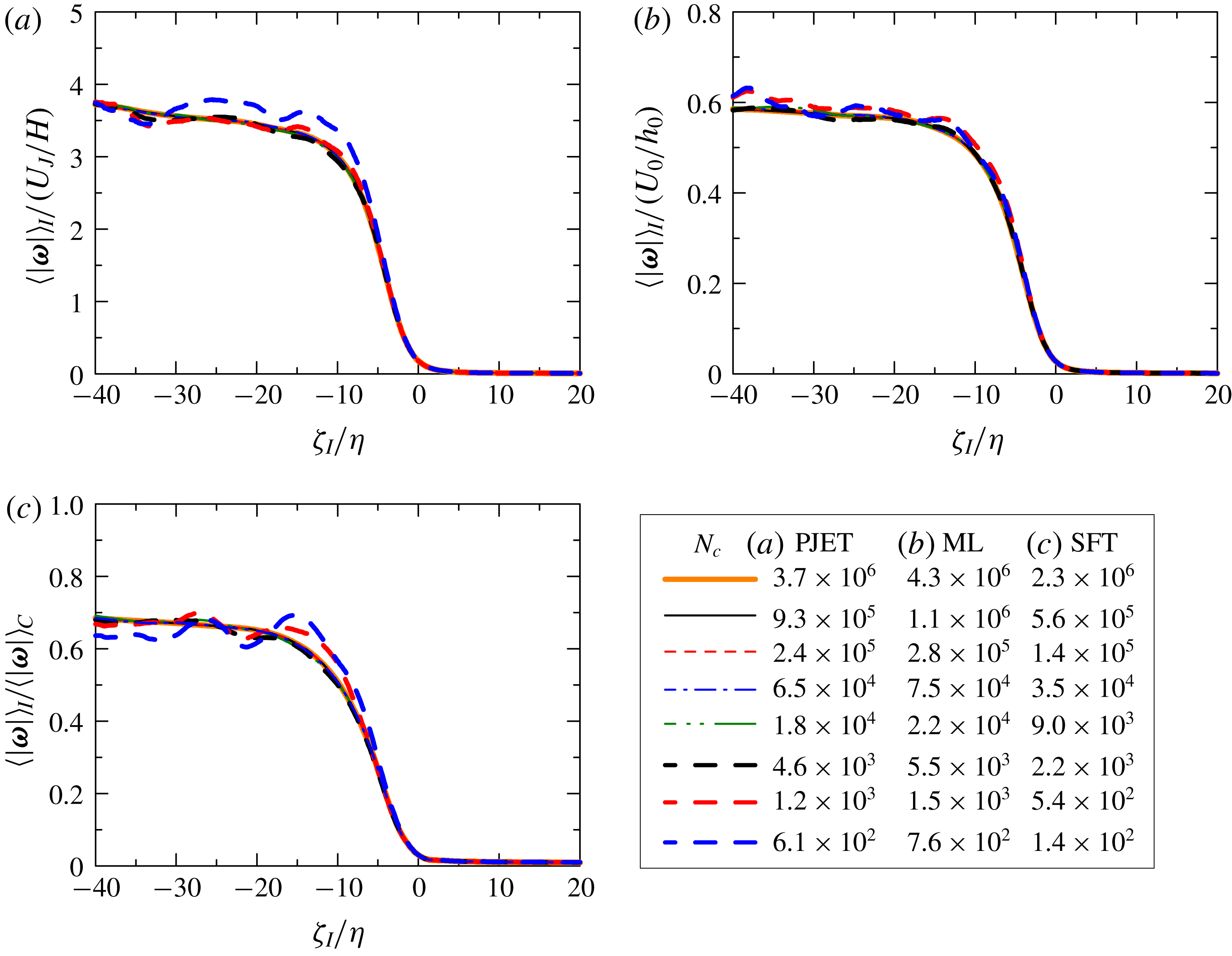
Influence of the number of samples on the conditional mean vorticity magnitude
 $\langle |\unicode[STIX]{x1D74E}|\rangle _{I}$
in cases (a) PJET, (b) ML and (c) SFT. In (c),
 $\langle |\unicode[STIX]{x1D74E}|\rangle _{I}$
is normalized by the mean vorticity magnitude on the centreline
 $\langle |\unicode[STIX]{x1D74E}|\rangle _{C}$
.
The number of samples used in the conditional profiles increases with the number of points,
 $N_{c}$
, on the isosurface of
 $|\unicode[STIX]{x1D74E}|=\unicode[STIX]{x1D714}_{th}$
used for setting the local coordinate, from which the samples are taken. Figure 2 compares the conditional mean vorticity magnitude
 $\langle |\unicode[STIX]{x1D74E}|\rangle _{I}$
obtained for a wide range of
 $N_{c}$
, where
 $\unicode[STIX]{x1D701}_{I}$
is normalized by the Kolmogorov scale
 $\unicode[STIX]{x1D702}$
on the centreline;
 $\langle |\unicode[STIX]{x1D74E}|\rangle _{I}$
decreases across the TNTI layer from the turbulent toward the non-turbulent region. As
 $N_{c}$
increases, the curve tends to collapse onto a single curve. The scatter due to a small number of samples is prominent for
 $N_{c}<10^{4}$
, while
 $\langle |\unicode[STIX]{x1D74E}|\rangle _{I}$
becomes independent of
 $N_{c}$
for
 $N_{c}>10^{4}$
. In the present study, the conditional statistics are computed with
 $N_{c}=3.5\times 10^{4}$
,
 $6.5\times 10^{4}$
and
 $7.5\times 10^{4}$
in the cases SFT, PJET and ML.
4 Scale decomposition near the turbulent/non-turbulent interface
4.1 Local spherical volume averages
In order to compute the turbulent characteristics near the TNTI layer, we use local volume averages in a sphere, denoted by an overbar, where for each sphere of radius
 $r$
centred at point
 $\boldsymbol{x}$
, a spherical volume average of a variable
 $\unicode[STIX]{x1D719}(\boldsymbol{x})$
is defined by (Watanabe & Nagata Reference Watanabe and Nagata2016),
 $$\begin{eqnarray}\displaystyle \overline{\unicode[STIX]{x1D719}}(\boldsymbol{x},r)=\frac{\displaystyle \iiint G(\boldsymbol{x},\boldsymbol{x}^{\prime },r)\unicode[STIX]{x1D719}(\boldsymbol{x}^{\prime })\,\text{d}\boldsymbol{x}^{\prime }}{V_{R}}=\frac{1}{N_{p}}\mathop{\sum }_{n=1}^{N_{p}}\unicode[STIX]{x1D719}[\boldsymbol{x}^{(n)}], & & \displaystyle\end{eqnarray}$$
where
 $V_{R}(r)$
is the volume of the sphere and
 $G(\boldsymbol{x})$
is a kernel function which is equal to 1 and 0 inside and outside of the sphere, respectively. This average corresponds to a low-pass filter operation with a cutoff length proportional to
 $r$
(Pumir, Shraiman & Chertkov Reference Pumir, Shraiman and Chertkov2001), whereby
 $\unicode[STIX]{x1D719}(\boldsymbol{x})$
can be decomposed into large-scale (
 $\overline{\unicode[STIX]{x1D719}}$
) and small-scale components (
 $\unicode[STIX]{x1D719}^{\prime \prime }$
), i.e.
 $\unicode[STIX]{x1D719}(\boldsymbol{x})=\overline{\unicode[STIX]{x1D719}}(\boldsymbol{x},r)+\unicode[STIX]{x1D719}^{\prime \prime }(\boldsymbol{x},r)$
. Here, a single length scale
 $r$
is used without distinguishing orientations.
In practice, the computation is carried out by taking
 $N_{p}$
fluid points randomly placed within the sphere, and by interpolating the value of the fluid variable
 $\unicode[STIX]{x1D719}(\boldsymbol{x})$
on each point
 $\boldsymbol{x}^{(n)}$
using a tri-linear interpolation, as indicated in the last term of the equation above. The number of points
 $N_{p}$
, used for each sphere of radius
 $r$
, is set as
 $N_{p}=\text{min}[(r/20\unicode[STIX]{x1D702})^{3},N_{lim}]$
, where the parameter
 $N_{lim}$
is chosen to limit the computational cost while
 $(r/20\unicode[STIX]{x1D702})^{3}$
ensures that the computational method used here is equivalent to the definition of the local volume average. When
 $(r/20\unicode[STIX]{x1D702})^{3}$
is smaller than 20,
 $N_{p}=20$
is used instead of
 $(r/20\unicode[STIX]{x1D702})^{3}$
. Additionally, an ensemble average of spheres,
 $\langle \overline{\unicode[STIX]{x1D719}}\rangle (r)$
, can be taken by using a large number of equally sized spheres located at different points
 $\boldsymbol{x}$
within the computational domain.
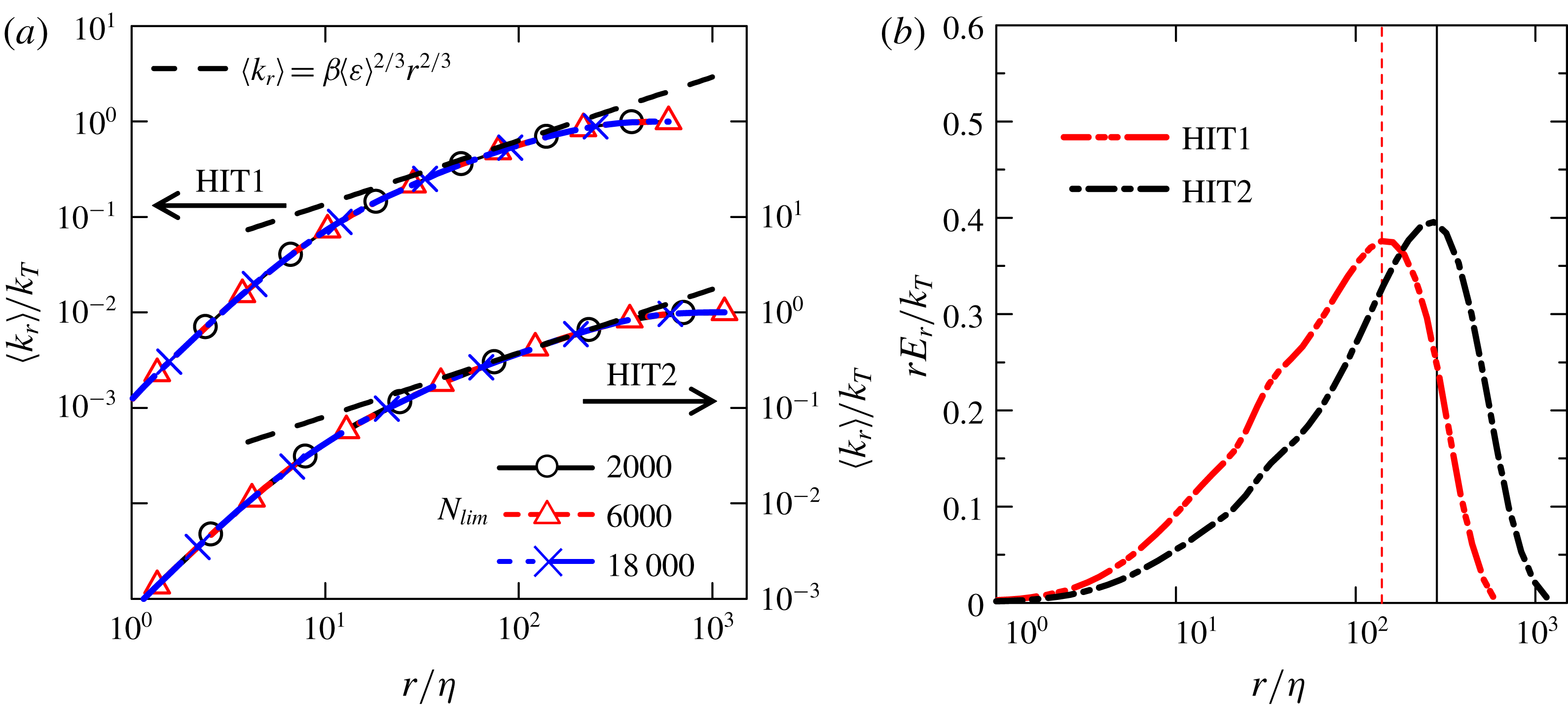
(a) Cumulative kinetic energy
 $\langle k_{r}\rangle$
normalized by the turbulent kinetic energy
 $k_{T}$
in cases HIT1 and HIT2 for several values of
 $N_{lim}$
. The theoretical curves
 $\unicode[STIX]{x1D6FD}\langle \unicode[STIX]{x1D700}\rangle ^{2/3}r^{2/3}$
(with
 $\unicode[STIX]{x1D6FD}=2$
) are also shown. (b) Contribution to the kinetic energy from scale
 $r$
,
 $rE_{r}$
, normalized by the turbulent kinetic energy
 $k_{T}$
.
We start by showing that using the new spherical volume average metric, one recovers the classical results observed in homogeneous isotropic turbulence. Specifically, we consider the kinetic energy averaged in a sphere,
 $k(\boldsymbol{x},r)=\overline{u_{i}(\boldsymbol{x})u_{i}(\boldsymbol{x})}/2$
, split into two contributions resulting from the spherical average:
 $k(\boldsymbol{x},r)=k_{m}(\boldsymbol{x},r)+k_{r}(\boldsymbol{x},r)$
, where
 $k_{m}(\boldsymbol{x},r)=\overline{u}_{i}\overline{u}_{i}/2$
involves the contribution from the sphere’s centre-of-mass (mean) motion, whereas
 $k_{r}(\boldsymbol{x},r)=\overline{u_{i}^{\prime \prime }u_{i}^{\prime \prime }}/2$
represents the contribution from (relative) motion in relation to the sphere’s centre of mass. From these definitions, one can interpret the ensemble average of
 $k_{r}(\boldsymbol{x},r)$
as the cumulative kinetic energy held in scales smaller than
 $r$
, such that
 $\langle k_{r}\rangle$
for large
 $r$
is equal to the turbulent kinetic energy
 $k_{T}=\langle u_{i}^{\prime }u_{i}^{\prime }\rangle /2$
. The brackets
 $\langle \,\,\rangle$
represent a spatial average. For computing
 $\langle k_{r}\rangle$
in homogeneous isotropic turbulence, the spatial average is taken with a large number of spheres (centred at different locations in the computational domain). Furthermore, a kinetic energy density at scale
 $r$
can be defined by
 $E_{r}=\unicode[STIX]{x2202}\langle k_{r}\rangle /\unicode[STIX]{x2202}r$
, whose integral gives the total kinetic energy as
 $k_{T}=\int _{0}^{\infty }E_{r}\,\text{d}r$
(Townsend Reference Townsend1976).
Figure 3(a) shows
 $\langle k_{r}\rangle$
in homogeneous isotropic turbulence (cases HIT1 and HIT2) for three different values of
 $N_{lim}$
;
 $\langle k_{r}\rangle$
increases with the radius of the sphere
 $r$
as expected from the definition, and for an intermediate range of
 $r$
, it closely follows the inertial range law
 $\langle k_{r}\rangle =\unicode[STIX]{x1D6FD}\langle \unicode[STIX]{x1D700}\rangle ^{2/3}r^{2/3}$
(with
 $\unicode[STIX]{x1D6FD}=2$
) predicted by Kolmogorov for the second-order velocity structure function (Davidson Reference Davidson2004), which is also a measure of the cumulative kinetic energy (Townsend Reference Townsend1976). Here, the broken line that represents
 $\langle k_{r}\rangle =\unicode[STIX]{x1D6FD}\langle \unicode[STIX]{x1D700}\rangle ^{2/3}r^{2/3}$
is obtained with
 $\langle \unicode[STIX]{x1D700}\rangle$
computed from the DNS results. The scale range with
 $\langle k_{r}\rangle =\unicode[STIX]{x1D6FD}\langle \unicode[STIX]{x1D700}\rangle ^{2/3}r^{2/3}$
is wider for HIT2, which has a higher Reynolds number than HIT1. It is clear that
 $\langle k_{r}\rangle$
is quite insensitive to the value of
 $N_{lim}$
provided that this number is sufficiently high, and a value of
 $N_{lim}=6000$
is therefore used for the rest of the paper.
Figure 3(b) shows
 $rE_{r}$
in semi-log coordinates, which represents the contribution to the turbulent kinetic energy from scale
 $r$
. It is expected that
 $rE_{r}$
peaks at the scale
 $r=L$
(Davidson Reference Davidson2004), where
 $L$
is the integral scale defined as
 $L=\int _{0}^{\infty }f(r)\,\text{d}r$
, where
 $f(r)=\langle u^{\prime }(x)u^{\prime }(x+r)\rangle /\langle {u^{\prime }}^{2}(x)\rangle$
is the longitudinal auto-correlation function. In the present simulations,
 $rE_{r}$
attain their maxima at
 $r=140\unicode[STIX]{x1D702}$
and
 $r=270\unicode[STIX]{x1D702}$
, for cases HIT1 and HIT2, respectively, which compare well with
 $L=140\unicode[STIX]{x1D702}$
and
 $L=265\unicode[STIX]{x1D702}$
(represented by the vertical lines in figure 3
b) directly obtained by integrating
 $f(r)$
for cases HIT1 and HIT2, respectively. Thus, we confirm using the present DNS that the integral scale can be obtained as the scale
 $r=L$
where
 $rE_{r}$
attains its maximum.
4.2 Conditional spherical volume averages
The local spherical volume averages are computed near the TNTI layer in relation to the position of the irrotational boundary. A volume average of ‘turbulent fluids’ on the local coordinate system is defined by extending the spherical volume average as
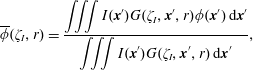 $$\begin{eqnarray}\displaystyle \overline{\unicode[STIX]{x1D719}}(\unicode[STIX]{x1D701}_{I},r)=\frac{\displaystyle \iiint I(\boldsymbol{x}^{\prime })G(\unicode[STIX]{x1D701}_{I},\boldsymbol{x}^{\prime },r)\unicode[STIX]{x1D719}(\boldsymbol{x}^{\prime })\,\text{d}\boldsymbol{x}^{\prime }}{\displaystyle \iiint I(\boldsymbol{x}^{\prime })G(\unicode[STIX]{x1D701}_{I},\boldsymbol{x}^{\prime },r)\,\text{d}\boldsymbol{x}^{\prime }}, & & \displaystyle\end{eqnarray}$$
where
 $I(\boldsymbol{x})$
is equal to 1 and 0 when the coordinate
 $\boldsymbol{x}$
is taken from the turbulent and non-turbulent regions, respectively. Introducing
 $\unicode[STIX]{x1D701}_{I}$
and
 $I(\boldsymbol{x})$
allows us to investigate the statistical properties of turbulence removing the contribution from non-turbulent fluid regions. An ensemble average is calculated with a large number of spheres (with radius
 $r$
) whose centres are located at a fixed distance
 $\unicode[STIX]{x1D701}_{I}$
from the irrotational boundary positions, where this average is denoted by
 $\langle \,\,\rangle _{RI}$
. The cumulative kinetic energy held below scale
 $r$
at a distance of
 $\unicode[STIX]{x1D701}_{I}$
from the irrotational boundary is denoted by
 $\langle k_{r}\rangle _{RI}(\unicode[STIX]{x1D701}_{I},r)$
. The advantage of the present metric is that it allows us to simultaneously assess the turbulent statistics as a function of the scale
 $r$
and of the position
 $\unicode[STIX]{x1D701}_{I}$
in relation to the TNTI. A classic low-pass filtering operation could also be used to perform a scale separation, however the filtering procedure would include flow points from both the turbulent and non-turbulent regions. Here we are interested in analysing the turbulent fluid near or within the TNTI layer while a sphere of radius
 $r$
at some location
 $\boldsymbol{x}$
may intersect the irrotational boundary at several points. Therefore, here the non-turbulent fluid is removed from these spherical averages. Thus, we can focus on the turbulent characteristics of the turbulent fluid near the irrotational boundary.
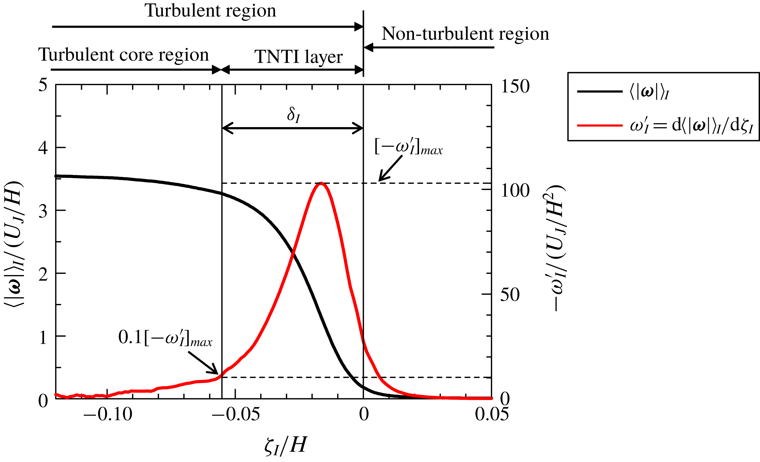
Conditional mean vorticity magnitude
 $\langle |\unicode[STIX]{x1D74E}|\rangle _{I}$
and its derivative with respective to
 $\unicode[STIX]{x1D701}_{I}$
,
 $\unicode[STIX]{x1D714}_{I}^{\prime }=\text{d}\langle |\unicode[STIX]{x1D74E}|\rangle _{I}/\text{d}\unicode[STIX]{x1D701}_{I}$
in PJET. The thickness of the TNTI layer is denoted by
 $\unicode[STIX]{x1D6FF}_{I}$
.
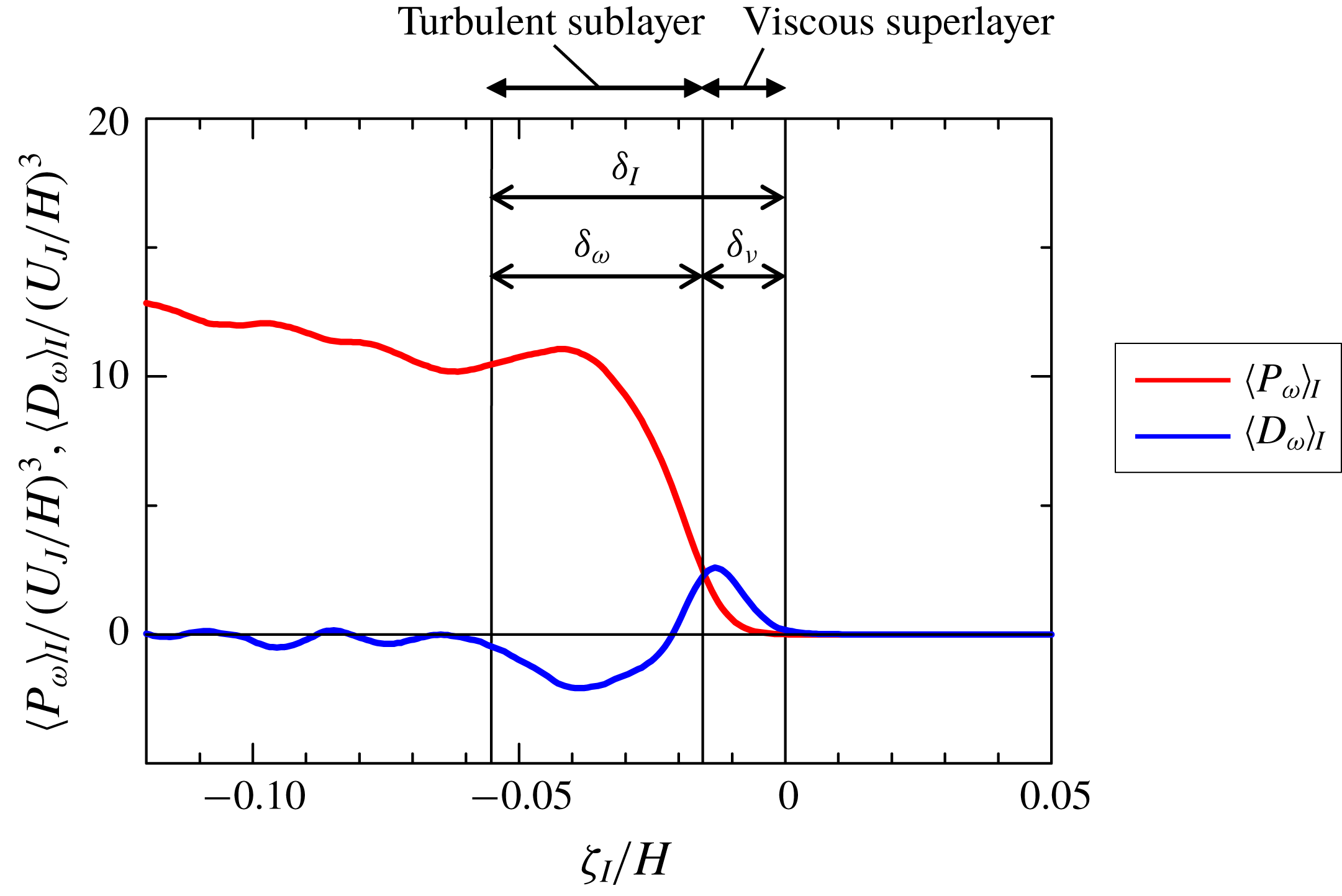
Conditional averages of enstrophy production term
 $\langle P_{\unicode[STIX]{x1D714}}\rangle _{I}$
and diffusion term
 $\langle D_{\unicode[STIX]{x1D714}}\rangle _{I}$
in PJET. The thicknesses of the turbulent sublayer and viscous superlayer are denoted by
 $\unicode[STIX]{x1D6FF}_{\unicode[STIX]{x1D714}}$
and
 $\unicode[STIX]{x1D6FF}_{\unicode[STIX]{x1D708}}$
, respectively.
5 Results and discussion
5.1 Conditional statistics near the TNTI layer
Figure 4 shows the conditional average of vorticity magnitude
 $\langle |\unicode[STIX]{x1D74E}|\rangle _{I}$
and its derivative
 $\unicode[STIX]{x1D714}_{I}^{\prime }=\text{d}\langle |\unicode[STIX]{x1D74E}|\rangle _{I}/\text{d}\unicode[STIX]{x1D701}_{I}$
with a negative sign in PJET;
 $\langle |\unicode[STIX]{x1D74E}|\rangle _{I}$
rapidly increases from the non-turbulent region (
 $\unicode[STIX]{x1D701}_{I}>0$
) toward the turbulent region (
 $\unicode[STIX]{x1D701}_{I}<0$
), and a peak of
 $-\unicode[STIX]{x1D714}_{I}^{\prime }$
appears at
 $\unicode[STIX]{x1D701}_{I}=-0.016H$
. The TNTI layer can be defined as the region across which the vorticity magnitude rapidly increases from the non-turbulent region toward the turbulent region. Following a previous study (Nagata, Watanabe & Nagata Reference Nagata, Watanabe and Nagata2018), the mean extent of the TNTI layer on the local coordinate can be quantified based on
 $\unicode[STIX]{x1D714}_{I}^{\prime }$
. Here, the outer edge of the TNTI layer is located at
 $\unicode[STIX]{x1D701}_{I}=0$
for the present choice of the threshold. The inner edge of the TNTI layer can be identified as the location at which
 $-\unicode[STIX]{x1D714}_{I}^{\prime }$
is equal to 10 % of the maximum value of
 $-\unicode[STIX]{x1D714}_{I}^{\prime }$
,
 $[-\unicode[STIX]{x1D714}_{I}^{\prime }]_{max}$
. The length between the outer and inner edges of the TNTI layer yields the thickness of the TNTI layer,
 $\unicode[STIX]{x1D6FF}_{I}$
, as shown in figure 4, where
 $\unicode[STIX]{x1D6FF}_{I}=0.055H$
is obtained. This method for estimating the TNTI layer thickness
 $\unicode[STIX]{x1D6FF}_{I}$
was compared with another method based on fitting an error function to conditional statistics in Watanabe et al. (Reference Watanabe, Riley, Nagata, Onishi and Matsuda2018a
), where both methods were shown to give a similar value of
 $\unicode[STIX]{x1D6FF}_{I}$
.
The inner structures of the TNTI layer, called the viscous superlayer and turbulent sublayer, are often discussed with respect to vorticity dynamics (van Reeuwijk & Holzner Reference van Reeuwijk and Holzner2014; da Silva et al. Reference da Silva, Hunt, Eames and Westerweel2014; Jahanbakhshi & Madnia Reference Jahanbakhshi and Madnia2018; Silva et al. Reference Silva, Zecchetto and da Silva2018). These inner layers can be detected by analysing the enstrophy transport equation
 $$\begin{eqnarray}\displaystyle \frac{D\unicode[STIX]{x1D714}^{2}/2}{Dt}=\unicode[STIX]{x1D714}_{i}S_{ij}\unicode[STIX]{x1D714}_{j}+\unicode[STIX]{x1D708}\unicode[STIX]{x1D6FB}^{2}(\unicode[STIX]{x1D714}^{2}/2)-\unicode[STIX]{x1D708}\unicode[STIX]{x1D735}\unicode[STIX]{x1D714}_{i}\boldsymbol{\cdot }\unicode[STIX]{x1D735}\unicode[STIX]{x1D714}_{i}=P_{\unicode[STIX]{x1D714}}+D_{\unicode[STIX]{x1D714}}+\unicode[STIX]{x1D700}_{\unicode[STIX]{x1D714}}, & & \displaystyle\end{eqnarray}$$
where
 $P_{\unicode[STIX]{x1D714}}=\unicode[STIX]{x1D714}_{i}S_{ij}\unicode[STIX]{x1D714}_{j}$
is the production term,
 $D_{\unicode[STIX]{x1D714}}=\unicode[STIX]{x1D708}\unicode[STIX]{x1D6FB}^{2}(\unicode[STIX]{x1D714}^{2}/2)$
is the viscous diffusion term and
 $\unicode[STIX]{x1D700}_{\unicode[STIX]{x1D714}}=-\unicode[STIX]{x1D708}\unicode[STIX]{x1D735}\unicode[STIX]{x1D714}_{i}\boldsymbol{\cdot }\unicode[STIX]{x1D735}\unicode[STIX]{x1D714}_{i}$
is the viscous dissipation term. When non-turbulent fluid is entrained into the TNTI layer,
 $\unicode[STIX]{x1D714}^{2}/2$
increases on the entrained fluid path through
 $P_{\unicode[STIX]{x1D714}}$
and
 $D_{\unicode[STIX]{x1D714}}$
. The conditional averages of
 $P_{\unicode[STIX]{x1D714}}$
and
 $D_{\unicode[STIX]{x1D714}}$
are shown for PJET in figure 5. Note that the conditional averages of
 $|\unicode[STIX]{x1D74E}|$
,
 $P_{\unicode[STIX]{x1D714}}$
and
 $D_{\unicode[STIX]{x1D714}}$
in a mixing layer and shear free turbulence are also similar to those in a planar jet (Watanabe et al.
Reference Watanabe, Sakai, Nagata, Ito and Hayase2015, Reference Watanabe, da Silva, Nagata and Sakai2017c
). Near the irrotational boundary (
 $\unicode[STIX]{x1D701}_{I}\approx 0$
), there is a region with
 $\langle P_{\unicode[STIX]{x1D714}}\rangle _{I}\leqslant \langle D_{\unicode[STIX]{x1D714}}\rangle _{I}$
, where the enstrophy growth is dominated by the viscous diffusion. This region is called the viscous superlayer (Taveira & da Silva Reference Taveira and da Silva2014). On the other hand,
 $\langle P_{\unicode[STIX]{x1D714}}\rangle _{I}$
exceeds
 $\langle D_{\unicode[STIX]{x1D714}}\rangle _{I}$
in the inner part of the TNTI layer, which is called turbulent sublayer (Silva et al.
Reference Silva, Zecchetto and da Silva2018). The mean thickness of the viscous superlayer
 $\unicode[STIX]{x1D6FF}_{\unicode[STIX]{x1D708}}$
can be obtained as the distance from
 $\unicode[STIX]{x1D701}_{I}=0$
to the location of
 $\langle P_{\unicode[STIX]{x1D714}}\rangle _{I}=\langle D_{\unicode[STIX]{x1D714}}\rangle _{I}$
. Then, the mean thickness of the turbulent sublayer,
 $\unicode[STIX]{x1D6FF}_{\unicode[STIX]{x1D714}}$
, can be obtained as
 $\unicode[STIX]{x1D6FF}_{\unicode[STIX]{x1D714}}=\unicode[STIX]{x1D6FF}_{I}-\unicode[STIX]{x1D6FF}_{\unicode[STIX]{x1D708}}$
. Values of
 $\unicode[STIX]{x1D6FF}_{\unicode[STIX]{x1D714}}$
and
 $\unicode[STIX]{x1D6FF}_{\unicode[STIX]{x1D708}}$
divided by Kolmogorov scale
 $\unicode[STIX]{x1D702}$
on the centreline (
 $y=0$
) are shown in table 1. Similar values of
 $\unicode[STIX]{x1D6FF}_{\unicode[STIX]{x1D714}}/\unicode[STIX]{x1D702}$
and
 $\unicode[STIX]{x1D6FF}_{\unicode[STIX]{x1D708}}/\unicode[STIX]{x1D702}$
were also reported in various flows (Silva et al.
Reference Silva, Zecchetto and da Silva2018; Zhang et al.
Reference Zhang, Watanabe and Nagata2018; Nagata et al.
Reference Nagata, Watanabe and Nagata2018), and agree with the scaling of the TNTI layer at high Reynolds numbers and of its sublayers, recently analysed in Silva et al. (Reference Silva, Zecchetto and da Silva2018).
Based on
 $\unicode[STIX]{x1D6FF}_{I}$
,
 $\unicode[STIX]{x1D6FF}_{\unicode[STIX]{x1D714}}$
and
 $\unicode[STIX]{x1D6FF}_{\unicode[STIX]{x1D708}}$
obtained in this way, the TNTI layer, viscous superlayer and turbulent sublayer, can be identified in the plots of conditional statistics as shown in figures 4 and 5. Furthermore, the turbulent region for
 $\unicode[STIX]{x1D701}_{I}\leqslant -\unicode[STIX]{x1D6FF}_{I}$
is called a turbulent core region in figure 5. Then, the local coordinate
 $\unicode[STIX]{x1D701}_{I}$
is divided into four regions: non-turbulent region, viscous superlayer, turbulent sublayer and turbulent core region. Identifying these regions is useful to interpret various statistics obtained near the TNTI layer. For example, the boundary between the viscous superlayer and turbulent sublayer was shown to have a large scalar dissipation rate and a high production rate of the scalar dissipation rate (Watanabe et al.
Reference Watanabe, Sakai, Nagata, Ito and Hayase2015). The movement of entrained fluid particles with respective to the irrotational boundary location was also shown to have different scalings between the turbulent sublayer and viscous superlayer (Watanabe et al.
Reference Watanabe, da Silva, Sakai, Nagata and Hayase2016b
). The turbulent sublayer also exhibits different statistical properties from the turbulent core region (e.g. alignment between the vorticity vector and eigenvectors of the strain tensor (Watanabe et al.
Reference Watanabe, Sakai, Nagata, Ito and Hayase2014)). For this reason, the conditional statistics are presented with marks that represent the boundaries between these four regions. It should be noted that the viscous terms are not dominant in the kinetic energy budget within the viscous superlayer. Pressure diffusion of kinetic energy also makes an important contribution to the kinetic energy budget within the TNTI layer (Taveira & da Silva Reference Taveira and da Silva2013; Terashima et al.
Reference Terashima, Sakai, Nagata, Ito, Onishi and Shouji2016; Watanabe et al.
Reference Watanabe, da Silva and Nagata2016a
).
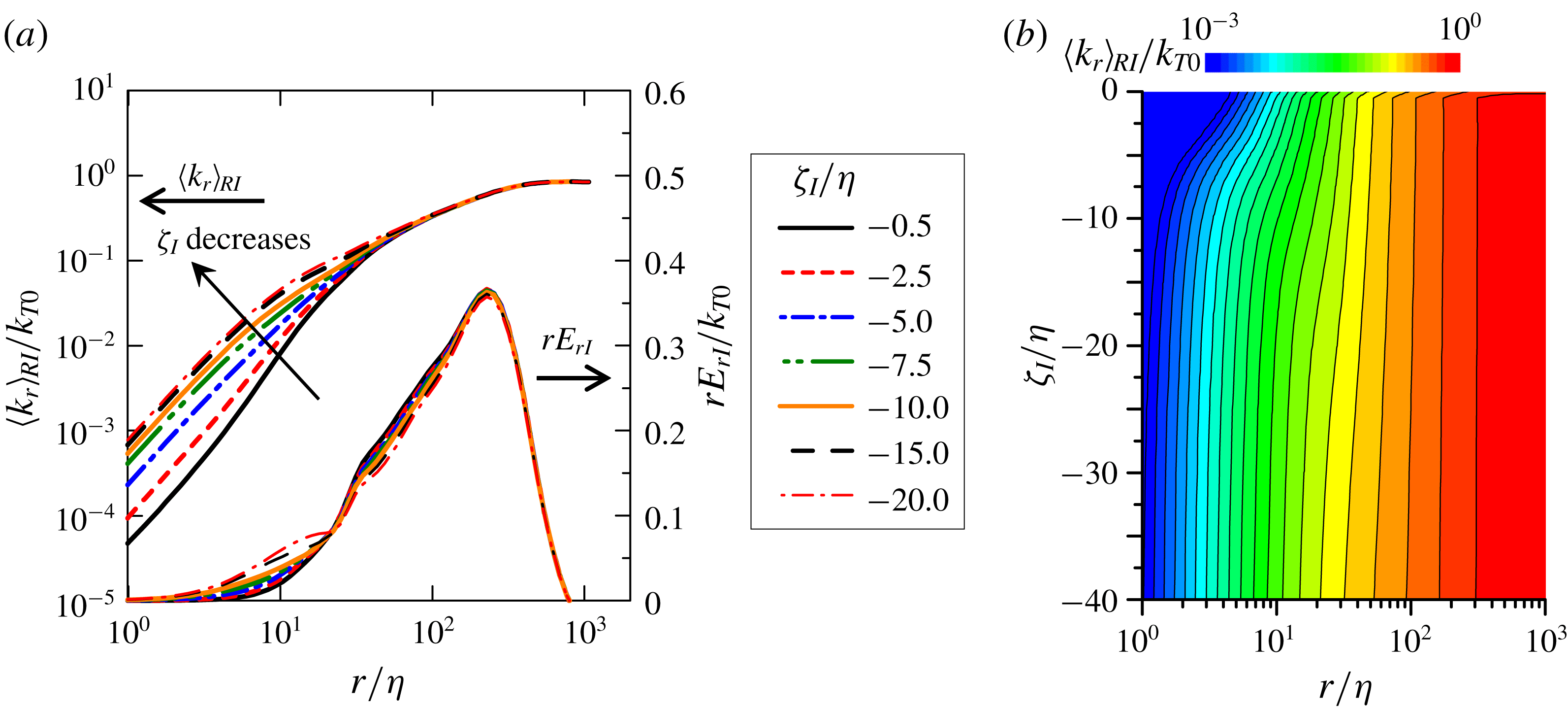
Conditional average of relative kinetic energy
 $\langle k_{r}\rangle _{RI}$
as a function of the distance
 $\unicode[STIX]{x1D701}_{I}$
from the irrotational boundary and the size of the sphere
 $r$
for shear free turbulence: (a) dependence on
 $r$
for several distances from the irrotational boundary,
 $-20\leqslant \unicode[STIX]{x1D701}_{I}/\unicode[STIX]{x1D702}\leqslant -0.5$
(the conditional energy density
 $rE_{rI}$
is also shown); (b) contours of
 $\langle k_{r}\rangle _{RI}$
on
 $(\unicode[STIX]{x1D701}_{I},r)$
for
 $-20\leqslant \unicode[STIX]{x1D701}_{I}/\unicode[STIX]{x1D702}\leqslant -0.5$
, and
 $10^{0}\leqslant r/\unicode[STIX]{x1D702}\leqslant 10^{3}$
.
 $\langle k_{r}\rangle _{RI}$
is normalized by the turbulent kinetic energy on the centreline of turbulence,
 $k_{T0}$
.
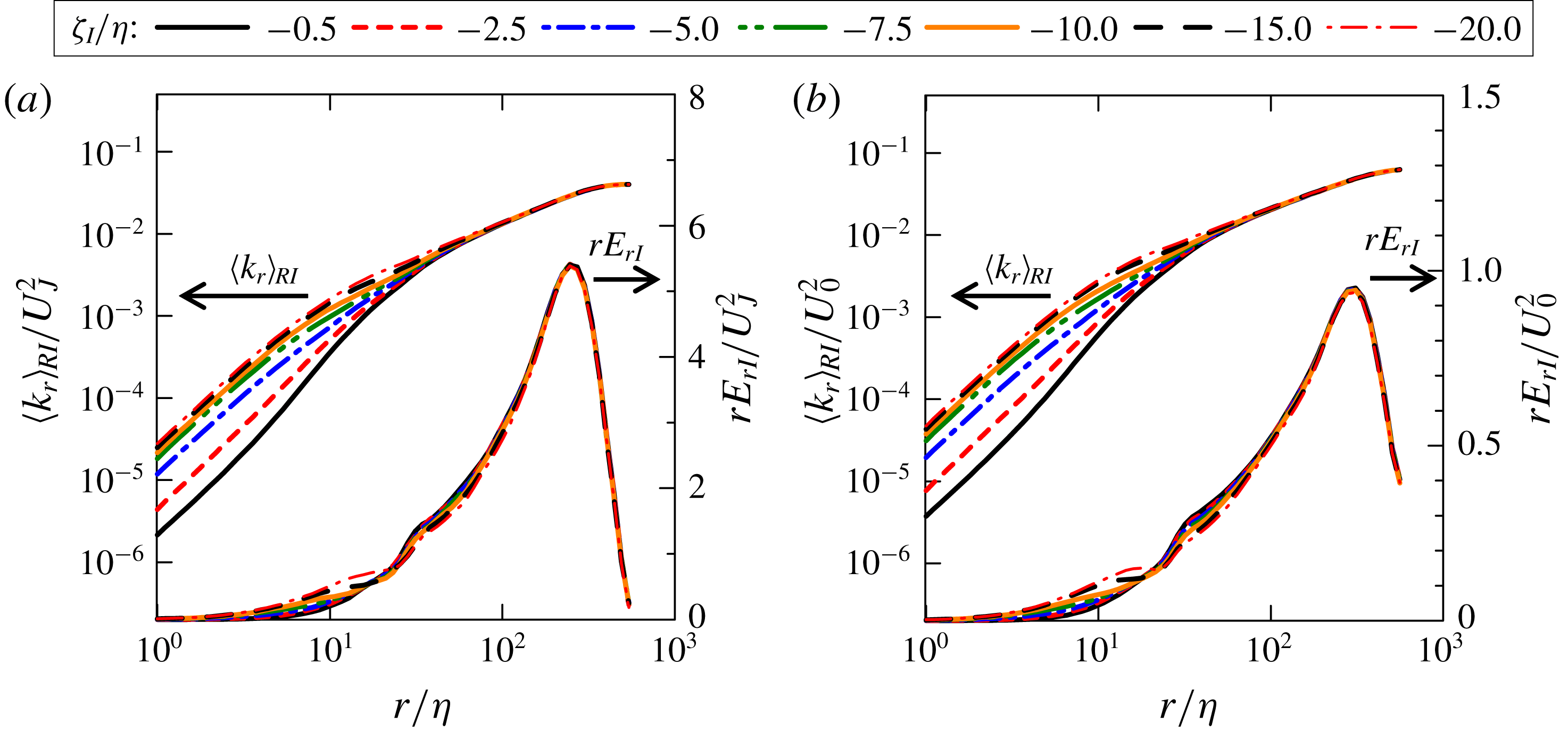
Conditional average of relative kinetic energy
 $\langle k_{r}\rangle _{RI}$
and conditional energy density
 $rE_{rI}$
in cases (a) PJET and (b) ML.
5.2 Conditional statistics with volume average near the TNTI layer
The conditional statistics are computed with the volume average (4.2) in the shear free turbulence, planar jet and mixing layer cases. Figure 6(a) plots the cumulative kinetic energy
 $\langle k_{r}\rangle _{RI}$
against
 $r/\unicode[STIX]{x1D702}$
obtained at different locations on
 $\unicode[STIX]{x1D701}_{I}$
in shear free turbulence while figure 6(b) shows a colour contour of
 $\langle k_{r}\rangle _{RI}$
as a function of
 $(r/\unicode[STIX]{x1D702},\unicode[STIX]{x1D701}_{I}/\unicode[STIX]{x1D702})$
. For
 $\unicode[STIX]{x1D701}_{I}/\unicode[STIX]{x1D702}>-10$
,
 $\langle k_{r}\rangle _{RI}$
for small
 $r$
notably decreases with
 $\unicode[STIX]{x1D701}_{I}$
, which indicates a depletion of kinetic energy at small scales within the TNTI layer. da Silva & Pereira (Reference da Silva and Pereira2008) showed that the irrotational motions outside the irrotational boundary are dominated by the large scales. However, the cumulative kinetic energy further shows that the energy distribution across scales begins to change within the TNTI layer. As in homogeneous isotropic turbulence, the integral scale of turbulence near the TNTI layer is estimated using the kinetic energy density
 $E_{rI}=\unicode[STIX]{x2202}\langle k_{r}\rangle _{RI}/\unicode[STIX]{x2202}r$
premultiplied by
 $r$
as shown in figure 6(a). The peak location of
 $rE_{r}$
that yields the integral length scale near the TNTI layer,
 $L_{I}$
, is insensitive to
 $\unicode[STIX]{x1D701}_{I}$
, in agreement with the rapid distortion theory applied for the TNTI layer (Teixeira & da Silva Reference Teixeira and da Silva2012).
Figure 7 shows the cumulative kinetic energy
 $\langle k_{r}\rangle _{RI}$
and kinetic energy density
 $rE_{r}$
near the TNTI layer for cases PJET and ML. Here, the range of
 $r$
is chosen to present the results for the length scales from the Kolmogorov scale
 $r/\unicode[STIX]{x1D702}=1$
to the length scale of the peak in
 $rE_{r}$
. The dependence of
 $\langle k_{r}\rangle _{RI}$
and
 $rE_{r}$
on
 $r$
and
 $\unicode[STIX]{x1D701}_{I}$
is similar for all flows. The cumulative kinetic energy
 $\langle k_{r}\rangle _{RI}$
in small scales decreases as
 $\unicode[STIX]{x1D701}_{I}$
becomes close to 0, and small-scale motions are less active as the irrotational boundary
 $\unicode[STIX]{x1D701}_{I}=0$
is approached from the turbulent region. The scale at which
 $rE_{r}$
peaks hardly depends on
 $\unicode[STIX]{x1D701}_{I}$
in the planar jet and mixing layer. The integral length scale
 $L_{I}$
at each
 $\unicode[STIX]{x1D701}_{I}$
can be obtained as the length
 $r$
at which
 $rE_{r}$
peaks, where
 $rE_{r}$
is computed for a wide range of
 $r$
and
 $\unicode[STIX]{x1D701}_{I}$
. However,
 $L_{I}$
does not change with
 $\unicode[STIX]{x1D701}_{I}$
as confirmed from the peak in
 $rE_{r}$
in figures 6(a) and 7. The values of
 $L_{I}$
in the shear free turbulence, planar jet and mixing layer are
 $L_{I}=1.9L_{0}$
,
 $L_{I}=1.0H=2.0L_{0}$
and
 $L_{I}=9.9h_{0}=2.3L_{0}$
, respectively, where
 $L_{0}$
is the integral length scale at
 $y=0$
, obtained by integrating the longitudinal auto-correlation function of the velocity fluctuation in the
 $x$
direction.
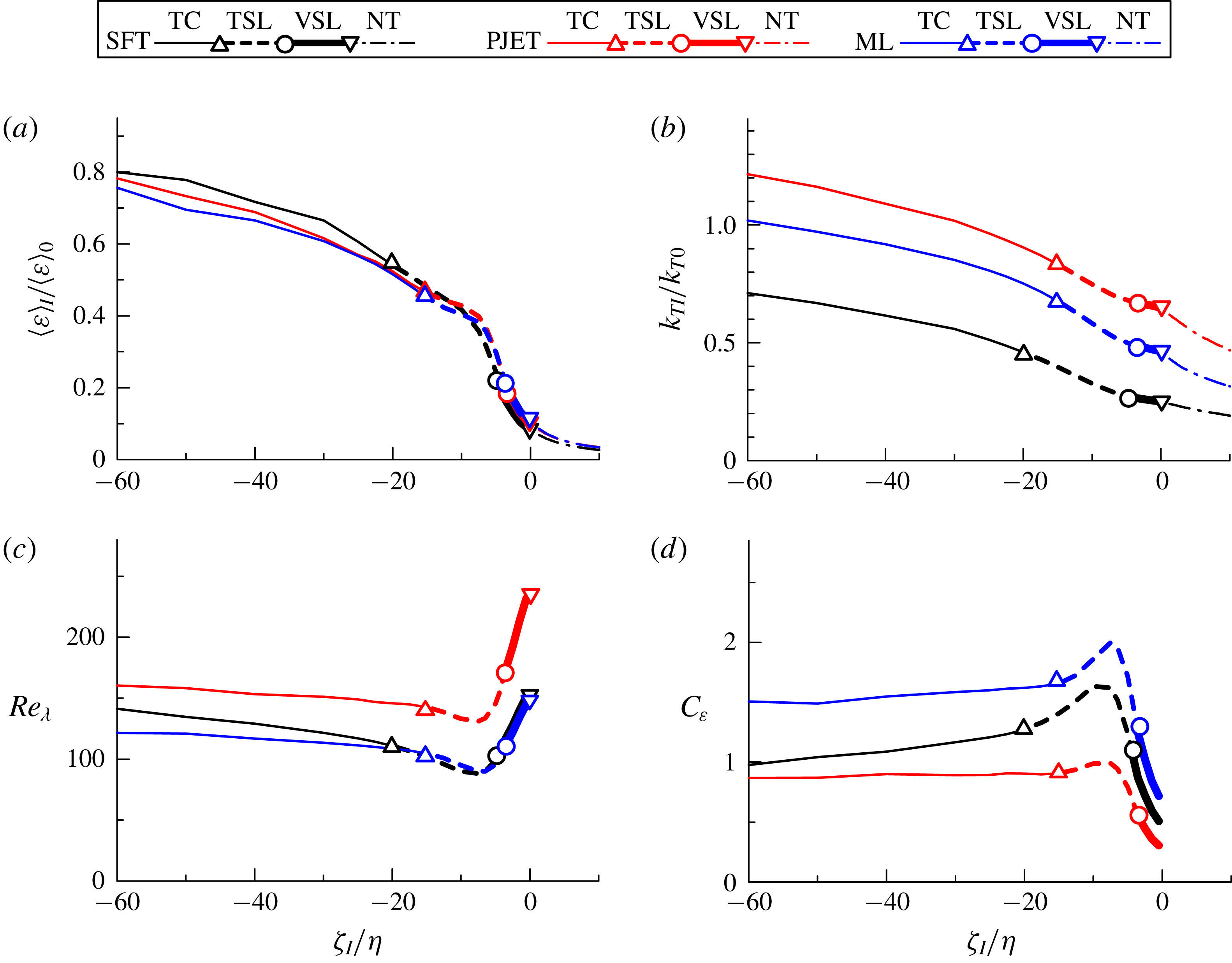
Conditional statistics in relation to the irrotational boundary: (a) averaged viscous dissipation rate
 $\unicode[STIX]{x1D700}$
; (b) turbulent kinetic energy
 $k_{TI}$
; (c) turbulent Reynolds number
 $Re_{\unicode[STIX]{x1D706}}$
; (d) non-dimensional dissipation rate
 $C_{\unicode[STIX]{x1D700}}$
. Different lines highlight the two sublayers that exist within the TNTI layer between the turbulent core (TC) and the non-turbulent region (NT): the viscous superlayer (VSL) and turbulent sublayer (TSL). Subscript 0 denotes the value taken at the centre of turbulence (
 $y=0$
).
5.3 Non-dimensional dissipation rate near the TNTI layer
The non-dimensional dissipation rate in free shear flows has been studied on the centreline of the flow, where it is calculated with the averaged energy dissipation rate and turbulent kinetic energy (or root-mean-squared streamwise velocity fluctuation) defined as one-point statistics and with the integral length scale computed with an auto-correlation function (Antonia et al.
Reference Antonia, Satyaprakash and Hussain1980; Deo et al.
Reference Deo, Mi and Nathan2008, Reference Deo, Nathan and Mi2013; Takamure et al.
Reference Takamure, Sakai, Ito, Iwano and Hayase2019). Similarly, the non-dimensional dissipation rate near the TNTI layer is calculated with the averaged kinetic energy dissipation rate
 $\langle \unicode[STIX]{x1D700}\rangle _{I}$
, turbulent kinetic energy
 $k_{TI}=(\langle u_{j}u_{j}\rangle _{I}-\langle u_{j}\rangle _{I}\langle u_{j}\rangle _{I})/2$
and the integral length scale
 $L_{I}$
, where
 $\langle \unicode[STIX]{x1D700}\rangle _{I}$
and
 $k_{TI}$
are obtained as one-point statistics on the local coordinate. Figure 8(a–c) shows
 $\langle \unicode[STIX]{x1D700}\rangle _{I}$
,
 $k_{TI}$
and the turbulent Reynolds number
 $Re_{\unicode[STIX]{x1D706}}=(2k_{TI}/3)^{1/2}\unicode[STIX]{x1D706}_{I}/\unicode[STIX]{x1D708}$
near the TNTI layer in the shear free turbulence, mixing layer and planar jet, where
 $\unicode[STIX]{x1D706}_{I}=\left(10\unicode[STIX]{x1D708}k_{TI}/\langle \unicode[STIX]{x1D700}\rangle _{I}\right)^{1/2}$
is the Taylor microscale. Note that the volume average (4.2) is not used for these quantities, and the conditional averages are simply taken on the local coordinate. Both
 $\langle \unicode[STIX]{x1D700}\rangle _{I}$
and
 $k_{TI}$
decrease when approaching the irrotational boundary from the turbulent region. However,
 $Re_{\unicode[STIX]{x1D706}}$
sharply increases in the viscous superlayer region and in the non-turbulent region, in agreement with Teixeira & da Silva (Reference Teixeira and da Silva2012).
The results from figures 8(a–c), 6(a) and 7 allow us to observe for the first time the non-dimensional energy dissipation rate
 $C_{\unicode[STIX]{x1D700}}$
near the TNTI layer. Figure 8(d) shows the profile of
 $C_{\unicode[STIX]{x1D700}}$
, which is computed directly from its definition as
 $\langle \unicode[STIX]{x1D700}\rangle _{I}L_{I}/(2k_{TI}/3)^{3/2}$
. Here,
 $C_{\unicode[STIX]{x1D700}}$
is shown for the turbulent region since the integral length scale is obtained as a length scale of turbulence. In the turbulent core region,
 $C_{\unicode[STIX]{x1D700}}$
is roughly constant in the three flows with
 $1.0\lesssim \langle C_{\unicode[STIX]{x1D700}}\rangle _{I}\lesssim 1.5$
, which is close to the value of
 $C_{\unicode[STIX]{x1D700}}\approx 1.0$
observed for decaying isotropic turbulence (Sreenivasan Reference Sreenivasan1984). However,
 $C_{\unicode[STIX]{x1D700}}$
exhibits a peculiar evolution near the TNTI in all the flows studied here, rising into a peak roughly at the middle of the turbulent sublayer at
 $\unicode[STIX]{x1D701}_{I}/\unicode[STIX]{x1D702}\approx -10$
, before sharply decreasing inside the viscous superlayer.
Normalized energy dissipation rate
 $C_{\unicode[STIX]{x1D700}}$
as a function of the turbulent Reynolds number
 $Re_{\unicode[STIX]{x1D706}}$
in the viscous superlayer and turbulent sublayer: (a) a logarithmic plot of
 $(C_{\unicode[STIX]{x1D700}},Re_{\unicode[STIX]{x1D706}})$
; (b) a linear plot of
 $(C_{\unicode[STIX]{x1D700}}Re_{\unicode[STIX]{x1D706}}^{2},Re_{\unicode[STIX]{x1D706}})$
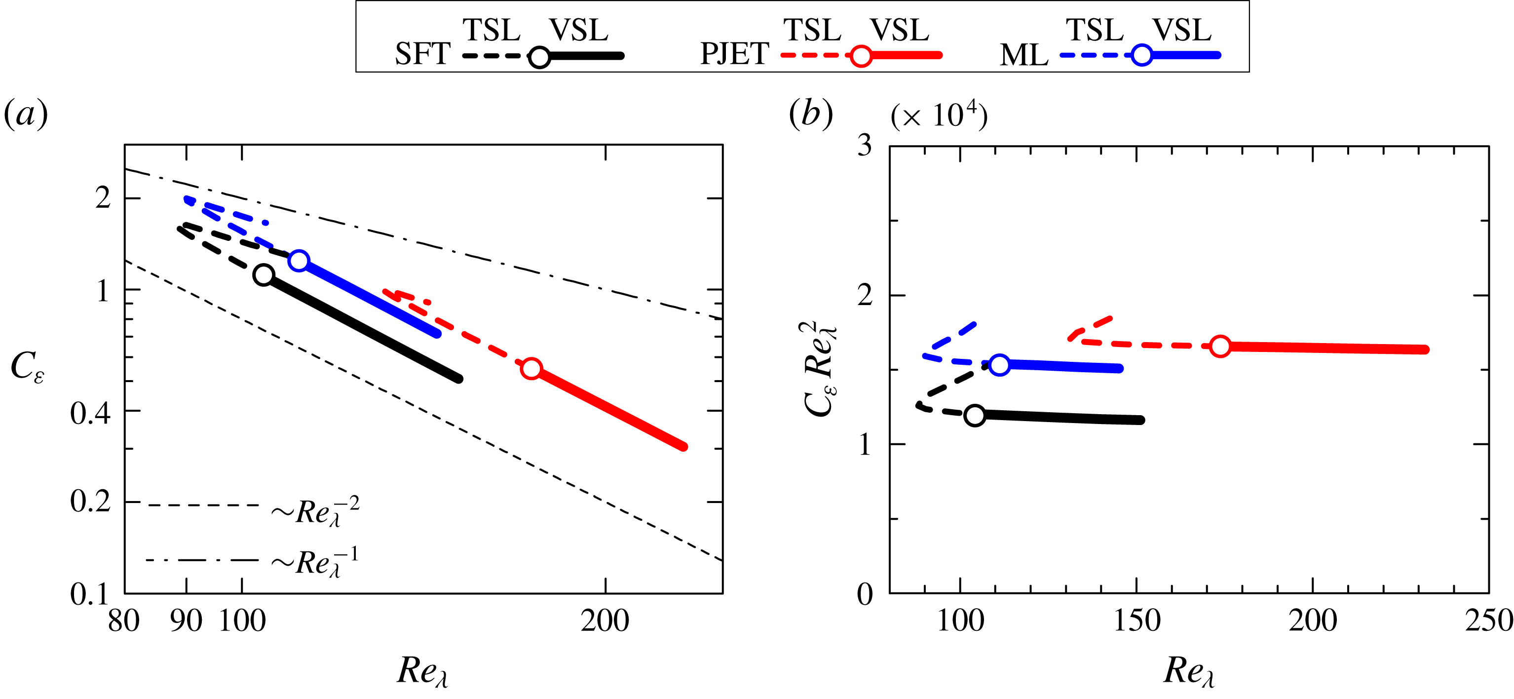
. Different lines are used for the turbulent sublayer (TSL) and viscous superlayer (VSL).
The spatial variation of
 $C_{\unicode[STIX]{x1D700}}$
is investigated in relation to the turbulent Reynolds number within the TNTI layer. Figure 9(a) plots
 $C_{\unicode[STIX]{x1D700}}$
against
 $Re_{\unicode[STIX]{x1D706}}$
in the turbulent sublayer and viscous superlayer. As
 $Re_{\unicode[STIX]{x1D706}}$
decreases from the viscous superlayer toward the turbulent sublayer,
 $C_{\unicode[STIX]{x1D700}}$
increases, where a power law
 $C_{\unicode[STIX]{x1D700}}\sim Re_{\unicode[STIX]{x1D706}}^{-2}$
is clearly found for all flows. Figure 9(b) plots
 $C_{\unicode[STIX]{x1D700}}$
premultiplied by
 $Re_{\unicode[STIX]{x1D706}}^{2}$
against
 $Re_{\unicode[STIX]{x1D706}}$
to confirm the relation
 $C_{\unicode[STIX]{x1D700}}\sim Re_{\unicode[STIX]{x1D706}}^{-2}$
, which appears as a horizontal line, and shows that the relation
 $C_{\unicode[STIX]{x1D700}}\sim Re_{\unicode[STIX]{x1D706}}^{-2}$
holds from the viscous superlayer to the middle of the turbulent sublayer. Clearly the relation
 $C_{\unicode[STIX]{x1D700}}\sim Re_{\unicode[STIX]{x1D706}}^{-2}$
arises mainly from the viscous superlayer, where viscous effects dominate enstrophy. The fact that the same relation is observed in a part of the turbulent sublayer is not easy to explain. The concepts of the viscous superlayer and turbulent sublayer are defined in relation to the enstrophy, which is a small-scale quantity, unlike the velocity, which impacts in the definition of
 $C_{\unicode[STIX]{x1D700}}$
. Clearly, from its definition, the viscous superlayer is dominated by enstrophy viscous diffusion. On the other hand, enstrophy production is dominant in the enstrophy growth in the turbulent sublayer. However, in practice there is of course a small overlap between the two effects – viscous diffusion and production – at the boundary between the viscous superlayer and turbulent sublayer, i.e. viscous effects do not end abruptly when we move from the viscous superlayer into the turbulent sublayer. To complicate matters,
 $C_{\unicode[STIX]{x1D700}}$
depends not only on the small scales but also on the velocity fluctuations associated with the large scales of motion with no direct link to the definition of the two sublayers, which is related to the small scales. The origin of
 $C_{\unicode[STIX]{x1D700}}\sim Re_{\unicode[STIX]{x1D706}}^{-2}$
is discussed further below and in the Appendix.
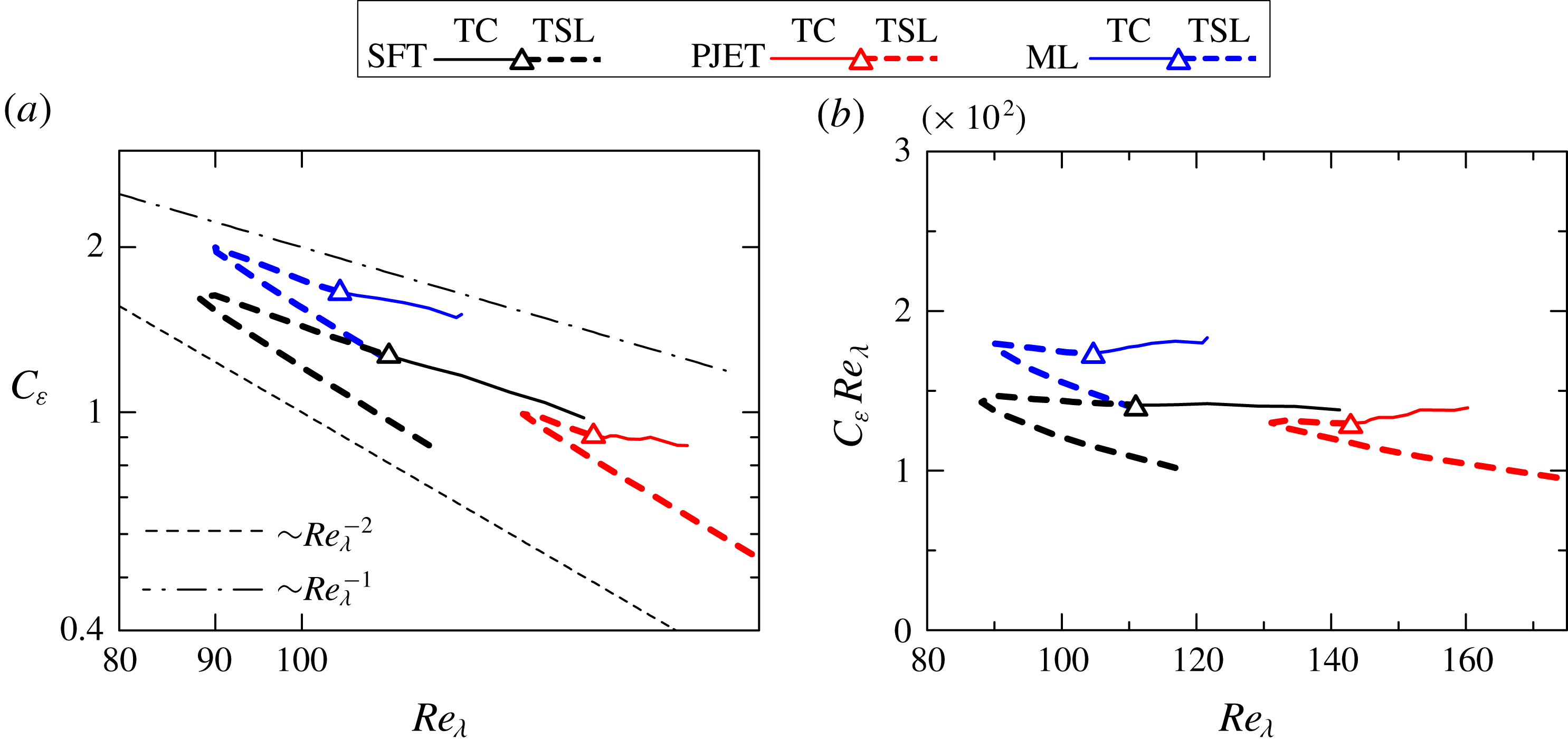
Figure 10(a) plots
 $C_{\unicode[STIX]{x1D700}}$
against
 $Re_{\unicode[STIX]{x1D706}}$
in the turbulent sublayer and turbulent core region. At the local minimum of
 $Re_{\unicode[STIX]{x1D706}}$
found in the turbulent sublayer (in figure 8
c), the relation between
 $C_{\unicode[STIX]{x1D700}}$
and
 $Re_{\unicode[STIX]{x1D706}}$
is changed, and
 $C_{\unicode[STIX]{x1D700}}\sim Re_{\unicode[STIX]{x1D706}}^{-1}$
follows in the rest of the turbulent sublayer. Figure 10(b) plots
 $C_{\unicode[STIX]{x1D700}}Re_{\unicode[STIX]{x1D706}}$
against
 $Re_{\unicode[STIX]{x1D706}}$
for confirming the relation
 $C_{\unicode[STIX]{x1D700}}\sim Re_{\unicode[STIX]{x1D706}}^{-1}$
, and thus
 $C_{\unicode[STIX]{x1D700}}Re_{\unicode[STIX]{x1D706}}$
tends to be constant in the turbulent sublayer and turbulent core region. The relation
 $C_{\unicode[STIX]{x1D700}}\sim Re_{\unicode[STIX]{x1D706}}^{-1}$
was also observed in non-equilibrium turbulence (Vassilicos Reference Vassilicos2015).
Normalized energy dissipation rate
 $C_{\unicode[STIX]{x1D700}}$
as a function of the turbulent Reynolds number
 $Re_{\unicode[STIX]{x1D706}}$
in the turbulent sublayer and turbulent core region: (a) a logarithmic plot of
 $(C_{\unicode[STIX]{x1D700}},Re_{\unicode[STIX]{x1D706}})$
; (b) a linear plot of
 $(C_{\unicode[STIX]{x1D700}}Re_{\unicode[STIX]{x1D706}},Re_{\unicode[STIX]{x1D706}})$
. Different lines are used for the turbulent core (TC) and turbulent sublayer (TSL).
In previous studies of non-equilibrium turbulence, the scaling
 $C_{\unicode[STIX]{x1D700}}\sim Re_{\unicode[STIX]{x1D706}}^{-1}$
has been explained via the influence of the large-scale coherent structures (Goto & Vassilicos Reference Goto and Vassilicos2016) or as a non-equilibrium perturbation correction to the Kolmogorov equilibrium spectrum (Bos & Rubinstein Reference Bos and Rubinstein2017). In the analysis of the TNTI layer, the relation
 $C_{\unicode[STIX]{x1D700}}\sim Re_{\unicode[STIX]{x1D706}}^{-1}$
is observed here for three very different flows, which have different large-scale structures and it is unclear how spectral spikes described in Goto & Vassilicos (Reference Goto and Vassilicos2016) could explain this scaling. Recall that in the shear free turbulence case, the typical large-scale eddies are somehow different from the ones observed in other flows, such as free shear flows. It is noteworthy that the energy spectra of streamwise velocity fluctuations in the temporally evolving mixing layer and planar jet, observed in previous studies, did not show any clear spikes at the large scales (Watanabe, Nagata & da Silva Reference Watanabe, Nagata and da Silva2017b
; Watanabe & Nagata Reference Watanabe and Nagata2017a
), but we cannot completely rule out the possible influence of these spikes that might exist in the early times of the simulations. On the other hand, the analysis considered in Bos & Rubinstein (Reference Bos and Rubinstein2017) is for relatively small perturbations, whereas the perturbations found within the turbulent sublayer are not likely small, since there are many possible reasons for perturbations being induced in the vicinity of the TNTI layer. For example, it was shown that the kinetic energy near the TNTI layer is transferred in physical space by pressure diffusion, whose contribution depends on the associated length scales (Taveira & da Silva Reference Taveira and da Silva2013; Terashima et al.
Reference Terashima, Sakai, Nagata, Ito, Onishi and Shouji2016; Watanabe et al.
Reference Watanabe, da Silva and Nagata2016a
). As suggested by an anonymous referee it is also possible that none of these explanations can be used to describe the observed relation
 $C_{\unicode[STIX]{x1D700}}\sim Re_{\unicode[STIX]{x1D706}}^{-1}$
. What is clear at the moment is that this scaling law is robust and is consistently observed in the turbulent sublayer of very different flow configurations.
Influences of the threshold
 $\unicode[STIX]{x1D714}_{th}$
used for detecting the irrotational boundary in PJET.
 $C_{\unicode[STIX]{x1D700}}$
plotted against (a)
 $\unicode[STIX]{x1D701}_{I}/\unicode[STIX]{x1D702}$
and (b)
 $Re_{\unicode[STIX]{x1D706}}$
for
 $\unicode[STIX]{x1D714}_{th}=0.9\unicode[STIX]{x1D714}_{th0}$
,
 $\unicode[STIX]{x1D714}_{th0}$
and
 $1.1\unicode[STIX]{x1D714}_{th0}$
, where
 $\unicode[STIX]{x1D714}_{th0}=0.18(U_{J}/H)$
is used in the present analysis.
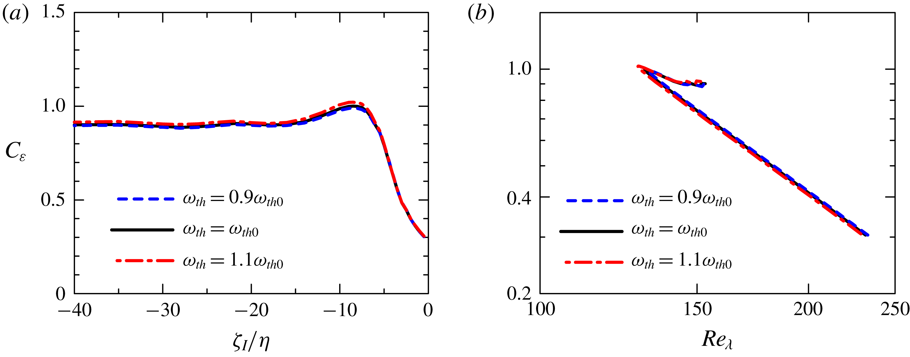
Figure 6 shows that the integral length scale
 $L_{I}$
is almost constant near the TNTI layer. In figures 8(a) and 8(b), although both averaged energy dissipation rate
 $\langle \unicode[STIX]{x1D700}\rangle _{I}$
and turbulent kinetic energy
 $k_{TI}$
decrease in the turbulent region toward
 $\unicode[STIX]{x1D701}_{I}=0$
,
 $k_{TI}$
only weakly depends on
 $\unicode[STIX]{x1D701}_{I}$
within the viscous superlayer. The assumption of constant
 $L_{I}$
and
 $k_{TI}$
yields
 $C_{\unicode[STIX]{x1D700}}\sim Re_{\unicode[STIX]{x1D706}}^{-2}$
from the definitions of
 $C_{\unicode[STIX]{x1D700}}$
and
 $Re_{\unicode[STIX]{x1D706}}$
, where
 $C_{\unicode[STIX]{x1D700}}=\langle \unicode[STIX]{x1D700}\rangle _{I}L_{I}/(2k_{TI}/3)^{3/2}$
and
 $Re_{\unicode[STIX]{x1D706}}=(20/3\unicode[STIX]{x1D708})^{1/2}k_{TI}\langle \unicode[STIX]{x1D700}\rangle _{I}^{-1/2}$
can be combined to give
 $C_{\unicode[STIX]{x1D700}}Re_{\unicode[STIX]{x1D706}}^{2}=CL_{I}\sqrt{k_{TI}}/\unicode[STIX]{x1D708}$
with constant
 $C$
. Therefore, the power law
 $C_{\unicode[STIX]{x1D700}}\sim Re_{\unicode[STIX]{x1D706}}^{-2}$
observed in the viscous superlayer and turbulent sublayer is related to the faster decay of
 $\langle \unicode[STIX]{x1D700}\rangle _{I}$
with
 $\unicode[STIX]{x1D701}_{I}$
, than those of
 $L_{I}$
and
 $k_{TI}$
, as discussed in the Appendix.
Finally, figure 11 shows
 $C_{\unicode[STIX]{x1D700}}$
plotted with
 $\unicode[STIX]{x1D701}_{I}/\unicode[STIX]{x1D702}$
and
 $Re_{\unicode[STIX]{x1D706}}$
obtained for different thresholds
 $\unicode[STIX]{x1D714}_{th}$
for PJET. Here, the results are compared for
 $\unicode[STIX]{x1D714}_{th}=0.9\unicode[STIX]{x1D714}_{th0}$
,
 $\unicode[STIX]{x1D714}_{th0}$
and
 $1.1\unicode[STIX]{x1D714}_{th0}$
, where
 $\unicode[STIX]{x1D714}_{th0}=0.18(U_{J}/H)$
is used in the other figures. The threshold dependence is very small and we observe the same tendency in all these plots.
6 Conclusions
Direct numerical simulations of planar jet, mixing layer and shear free turbulence were used to study the non-dimensional dissipation rate
 $C_{\unicode[STIX]{x1D700}}$
, near the TNTI layer, where the turbulent Reynolds number
 $Re_{\unicode[STIX]{x1D706}}$
ranges between
 $120$
and
 $180$
at the centreline of the turbulent region of these flows. The analysis was made possible through the development of a new procedure based on a volume average within a sphere with radius
 $r$
, which allows a detailed investigation of the scale dependence of kinetic energy near the TNTI layer. For instance, the kinetic energy density at the scale
 $r$
can be computed by taking the derivative of the cumulative kinetic energy with respective to
 $r$
.
To validate this method based on the volume average, several well-known turbulent statistics were first recovered in homogeneous isotropic turbulence. The cumulative kinetic energy computed with the volume averaging procedure in homogeneous isotropic turbulence was shown to increase with
 $r^{2/3}$
for an intermediate range of scales
 $r$
, as expected from the scaling of the second-order velocity structure function. It was shown that the scale dependence of the kinetic energy density yields an integral length scale close to that obtained from the auto-correlation function of the velocity fluctuation.
The tools based on the volume average were combined with the conditional averages, as a function of the position within the TNTI layer
 $\unicode[STIX]{x1D701}_{I}$
. Here, the statistics were computed only for turbulent fluid regions, by eliminating non-turbulent fluids from the volume average. For all of the flows studied in the present work the kinetic energy at small scales becomes smaller as the irrotational boundary is approached (from the turbulent region). An important result was the realization that the turbulent integral length scale
 $L_{I}$
, estimated from the scale dependence of kinetic energy density, was shown to be almost independent of the position
 $\unicode[STIX]{x1D701}_{I}$
near the TNTI layer. The present method uses a single length scale
 $r$
without distinguishing orientations, and anisotropy of the integral length scale cannot be studied with this method.
The non-dimensional energy dissipation rate near the TNTI layer was computed as
 $C_{\unicode[STIX]{x1D700}}=\langle \unicode[STIX]{x1D700}\rangle _{I}L_{I}/(2k_{TI}/3)^{3/2}$
with the averaged viscous dissipation rate
 $\langle \unicode[STIX]{x1D700}\rangle _{I}$
and the turbulent kinetic energy
 $k_{TI}$
defined with the averages conditioned on
 $\unicode[STIX]{x1D701}_{I}$
. The results show that for all of the flows considered in this work, as the irrotational boundary is approached from the turbulent region,
 $C_{\unicode[STIX]{x1D700}}$
slightly increases and reaches its peak within the turbulent sublayer, and later decreases within the viscous superlayer. The value of
 $C_{\unicode[STIX]{x1D700}}$
plotted against the turbulent Reynolds number
 $Re_{\unicode[STIX]{x1D706}}$
showed that
 $C_{\unicode[STIX]{x1D700}}$
within the TNTI layer exhibits two relations:
 $C_{\unicode[STIX]{x1D700}}\sim Re_{\unicode[STIX]{x1D706}}^{-1}$
and
 $C_{\unicode[STIX]{x1D700}}\sim Re_{\unicode[STIX]{x1D706}}^{-2}$
. Specifically, whereas the viscous superlayer and part of the turbulent sublayer display
 $C_{\unicode[STIX]{x1D700}}\sim Re_{\unicode[STIX]{x1D706}}^{-2}$
, the remainder of the turbulent sublayer exhibits
 $C_{\unicode[STIX]{x1D700}}\sim Re_{\unicode[STIX]{x1D706}}^{-1}$
. The relation
 $C_{\unicode[STIX]{x1D700}}\sim Re_{\unicode[STIX]{x1D706}}^{-1}$
is consistent with the dissipation scaling observed in non-equilibrium turbulence (Vassilicos Reference Vassilicos2015).
Acknowledgements
This work was supported by JSPS KAKENHI grant numbers 18K13682 and 18H01367 and by ‘Collaborative Research Project on Computer Science with High-Performance Computing in Nagoya University’. C.B.d.S. acknowledges Fundação para a ciência e Tecnologia (FCT), under grant PTDC/EMS-ENE/6129/2014. Some of numerical simulations presented in this manuscript were carried out on the high-performance computing system (NEC SX-ACE) in the Japan Agency for Marine-Earth Science and Technology. The authors acknowledge the Laboratory for Advanced Computing at University of Coimbra for providing HPC, computing and consulting resources (http://www.lca.uc.pt).
Appendix
In this Appendix we compare how several flow variables evolve in HIT and within a TNTI layer by using results from the HIT1 and PJET simulations. The idea behind this comparison can be understood by recalling that when one moves from the irrotational into the turbulent region across the TNTI layer the local vorticity increases. Therefore, a conditional mean, made in relation to a distance from a fixed position within the TNTI layer, can be compared to a conditional mean made in relation to the local value of the enstrophy
 $\unicode[STIX]{x1D714}^{2}/2$
. This allows us to compare the evolution of several flow variables across the TNTI (from the irrotational to the turbulent region) to how they evolve in homogeneous isotropic turbulence, from regions of weak local enstrophy to regions of intense local enstrophy. Here the conditional averages (as functions of
 $\unicode[STIX]{x1D714}^{2}/2$
) used in HIT1 are denoted by
 $\langle \cdot \rangle _{\unicode[STIX]{x1D714}}$
, where the average is performed over space. The evolution of the variables within the TNTI layer in PJET is assessed with averages
 $\langle \cdot \rangle _{I}$
, where the local coordinate
 $\unicode[STIX]{x1D701}_{I}$
corresponds to a given mean enstrophy
 $\langle \unicode[STIX]{x1D714}^{2}/2\rangle _{I}$
, which of course increases across the TNTI layer. Thus, the average
 $\langle \cdot \rangle _{I}$
plotted against
 $\langle \unicode[STIX]{x1D714}^{2}/2\rangle _{I}$
for the same
 $\unicode[STIX]{x1D701}_{I}$
(in PJET) can be compared with the average
 $\langle \cdot \rangle _{\unicode[STIX]{x1D714}}$
plotted against
 $\unicode[STIX]{x1D714}^{2}/2$
for homogeneous isotropic turbulence (in HIT1). Notice that in PJET the viscous superlayer is formed at the outer edge of the turbulent region, where the enstrophy level is only slightly higher than in the non-turbulent region. In other words, in these conditional statistics the viscous superlayer and a part of the turbulent sublayer (for PJET) can be compared with the weak vorticity (small enstrophy) region of HIT1.
(a) Conditional averages on enstrophy for enstrophy diffusion and production terms,
 $\langle D_{\unicode[STIX]{x1D714}}\rangle _{\unicode[STIX]{x1D714}}$
and
 $\langle P_{\unicode[STIX]{x1D714}}\rangle _{\unicode[STIX]{x1D714}}$
, for HIT1.
 $\langle D_{\unicode[STIX]{x1D714}}\rangle _{\unicode[STIX]{x1D714}}$
and
 $\langle P_{\unicode[STIX]{x1D714}}\rangle _{\unicode[STIX]{x1D714}}$
are normalized by
 $\langle S_{ij}S_{ij}\rangle ^{3/2}$
while
 $\unicode[STIX]{x1D714}^{2}/2$
is divided by mean enstrophy
 $\langle \unicode[STIX]{x1D714}^{2}/2\rangle$
. (b)
 $\langle D_{\unicode[STIX]{x1D714}}\rangle _{I}$
and
 $\langle P_{\unicode[STIX]{x1D714}}\rangle _{I}$
plotted against
 $\langle \unicode[STIX]{x1D714}^{2}/2\rangle _{I}$
at the same location of
 $\unicode[STIX]{x1D701}_{I}$
within the TNTI layer in PJET. Different lines are used for the non-turbulent region (NT), viscous superlayer (VSL) and turbulent sublayer (TSL) in (b).
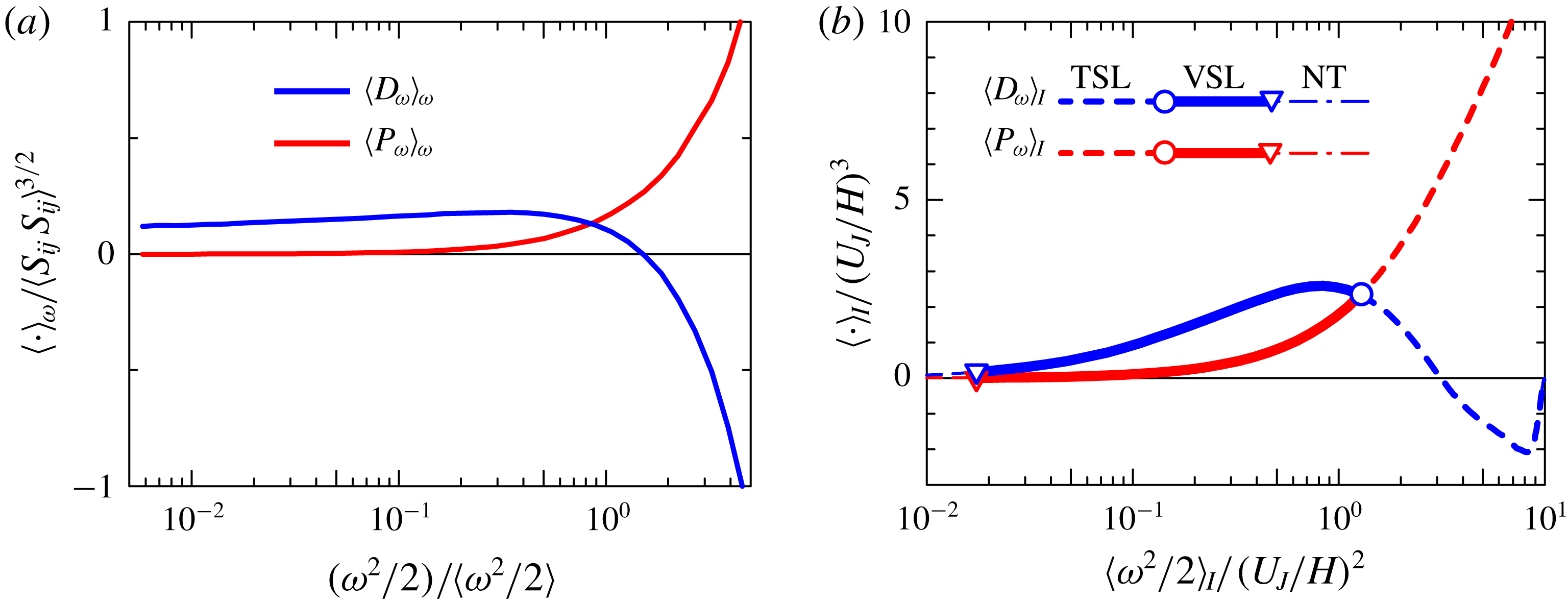
Figure 12(a) shows the averages, conditioned on enstrophy, of enstrophy diffusion and production,
 $\langle D_{\unicode[STIX]{x1D714}}\rangle _{\unicode[STIX]{x1D714}}$
and
 $\langle P_{\unicode[STIX]{x1D714}}\rangle _{\unicode[STIX]{x1D714}}$
, plotted against
 $\unicode[STIX]{x1D714}^{2}/2$
(divided by its mean value
 $\langle \unicode[STIX]{x1D714}^{2}/2\rangle$
) for HIT1. The diffusion term
 $\langle D_{\unicode[STIX]{x1D714}}\rangle _{\unicode[STIX]{x1D714}}$
exhibits negative and positive values for large and small values of
 $\unicode[STIX]{x1D714}^{2}/2$
, respectively, which indicates that the enstrophy is transferred from regions of large
 $\unicode[STIX]{x1D714}^{2}/2$
to regions with small
 $\unicode[STIX]{x1D714}^{2}/2$
, as expected. On the other hand, the production term
 $\langle P_{\unicode[STIX]{x1D714}}\rangle _{\unicode[STIX]{x1D714}}$
is close to 0 for small
 $\unicode[STIX]{x1D714}^{2}/2$
, but rapidly increases with the enstrophy for large
 $\unicode[STIX]{x1D714}^{2}/2$
, naturally expressing the dependence of the enstrophy production
 $P_{\unicode[STIX]{x1D714}}=\unicode[STIX]{x1D714}_{i}S_{ij}\unicode[STIX]{x1D714}_{j}$
on the enstrophy magnitude. Figure 12(b) shows
 $\langle D_{\unicode[STIX]{x1D714}}\rangle _{I}$
and
 $\langle P_{\unicode[STIX]{x1D714}}\rangle _{I}$
against
 $\langle \unicode[STIX]{x1D714}^{2}/2\rangle _{I}$
for PJET, where the associated
 $\unicode[STIX]{x1D701}_{I}$
is in the range transitioning from the non-turbulent region to the turbulent sublayer of the TNTI layer. In the viscous superlayer,
 $\langle D_{\unicode[STIX]{x1D714}}\rangle _{I}$
is positive and increases with
 $\langle \unicode[STIX]{x1D714}^{2}/2\rangle _{I}$
, before becoming negative within the turbulent sublayer. The production term
 $\langle P_{\unicode[STIX]{x1D714}}\rangle _{I}$
on the other hand is close to zero for small
 $\langle \unicode[STIX]{x1D714}^{2}/2\rangle _{I}$
(within the viscous superlayer), but it rapidly increases with
 $\langle \unicode[STIX]{x1D714}^{2}/2\rangle _{I}$
moving from the viscous superlayer to the turbulent sublayer, where the crossing between
 $\langle D_{\unicode[STIX]{x1D714}}\rangle _{I}$
and
 $\langle P_{\unicode[STIX]{x1D714}}\rangle _{I}$
takes place at the end of the viscous superlayer. This evolution of
 $\langle D_{\unicode[STIX]{x1D714}}\rangle _{I}$
and
 $\langle P_{\unicode[STIX]{x1D714}}\rangle _{I}$
in the TNTI layer is well documented in previous works, e.g. Taveira & da Silva (Reference Taveira and da Silva2014), but the similarities with homogeneous isotropic turbulence are new and interesting to observe (compare figures 12
a and 12
b). Regions of strong enstrophy in homogeneous isotropic turbulence are connected with the presence of intense vortices, which also somehow define the TNTI layer and can explain these similarities (Watanabe et al.
Reference Watanabe, Jaulino, Taveira, da Silva, Nagata and Sakai2017a
). Naturally, the similarities between the TNTI layer and homogeneous isotropic turbulence end when one considers regions of very low enstrophy. This is because the non-turbulent region with
 $\unicode[STIX]{x1D714}^{2}\approx 0$
is bounded by the outer edge of the viscous superlayer in the planar jet while low-
 $\unicode[STIX]{x1D714}^{2}$
regions in the homogeneous isotropic turbulence can be surrounded by fluid with much higher
 $\unicode[STIX]{x1D714}^{2}$
, from which enstrophy can be transferred towards the low-
 $\unicode[STIX]{x1D714}^{2}$
regions by the viscous diffusion. Also, differences arise for large values of enstrophy, e.g. when
 $\langle D_{\unicode[STIX]{x1D714}}\rangle _{I}$
is close to 0 at
 $\langle \unicode[STIX]{x1D714}^{2}/2\rangle _{I}/(U_{J}/H)^{2}\approx 10$
in figure 12(b), while
 $\langle D_{\unicode[STIX]{x1D714}}\rangle _{\unicode[STIX]{x1D714}}$
in figure 12(a) decreases with
 $\unicode[STIX]{x1D714}^{2}/2$
. The explanation is again simple. The average in the turbulent sublayer can contain fluid with a wide range of
 $\unicode[STIX]{x1D714}^{2}/2$
, because the enstrophy is highly intermittent in the turbulent region as shown in figure 1, and averaging turbulent fluids with various values of
 $\unicode[STIX]{x1D714}^{2}/2$
results in cancellation of both positive and negative
 $D_{\unicode[STIX]{x1D714}}$
in the averaged value
 $\langle D_{\unicode[STIX]{x1D714}}\rangle _{I}$
for large
 $\langle \unicode[STIX]{x1D714}^{2}/2\rangle _{I}$
(Jahanbakhshi & Madnia Reference Jahanbakhshi and Madnia2016; Zhang et al.
Reference Zhang, Watanabe and Nagata2018). Nevertheless, it is clear that the transition from the viscous superlayer to the turbulent sublayer as observed in figure 12(b) for
 $\langle D_{\unicode[STIX]{x1D714}}\rangle _{I}$
and
 $\langle P_{\unicode[STIX]{x1D714}}\rangle _{I}$
is similar to that observed in the homogeneous isotropic turbulence.
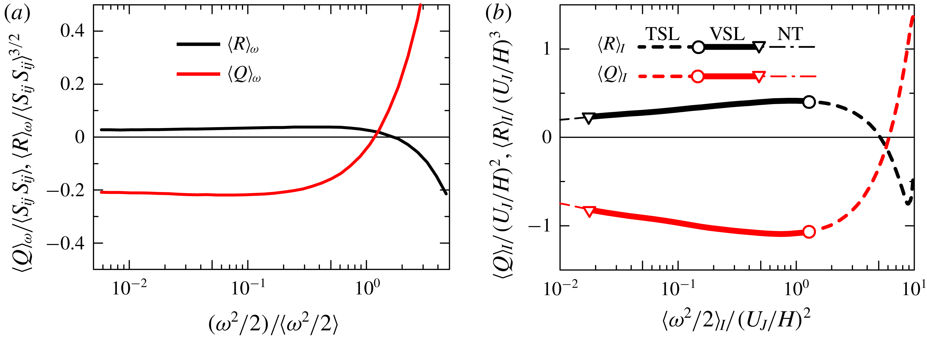
(a) Averages conditioned on enstrophy taken for second and third invariants of velocity gradient tensor (
 $Q$
and
 $R$
). (b)
 $\langle Q\rangle _{I}$
and
 $\langle R\rangle _{I}$
plotted against
 $\langle \unicode[STIX]{x1D714}^{2}/2\rangle _{I}$
within the TNTI layer in PJET. Different lines are used for the non-turbulent region (NT), viscous superlayer (VSL) and turbulent sublayer (TSL) in (b).
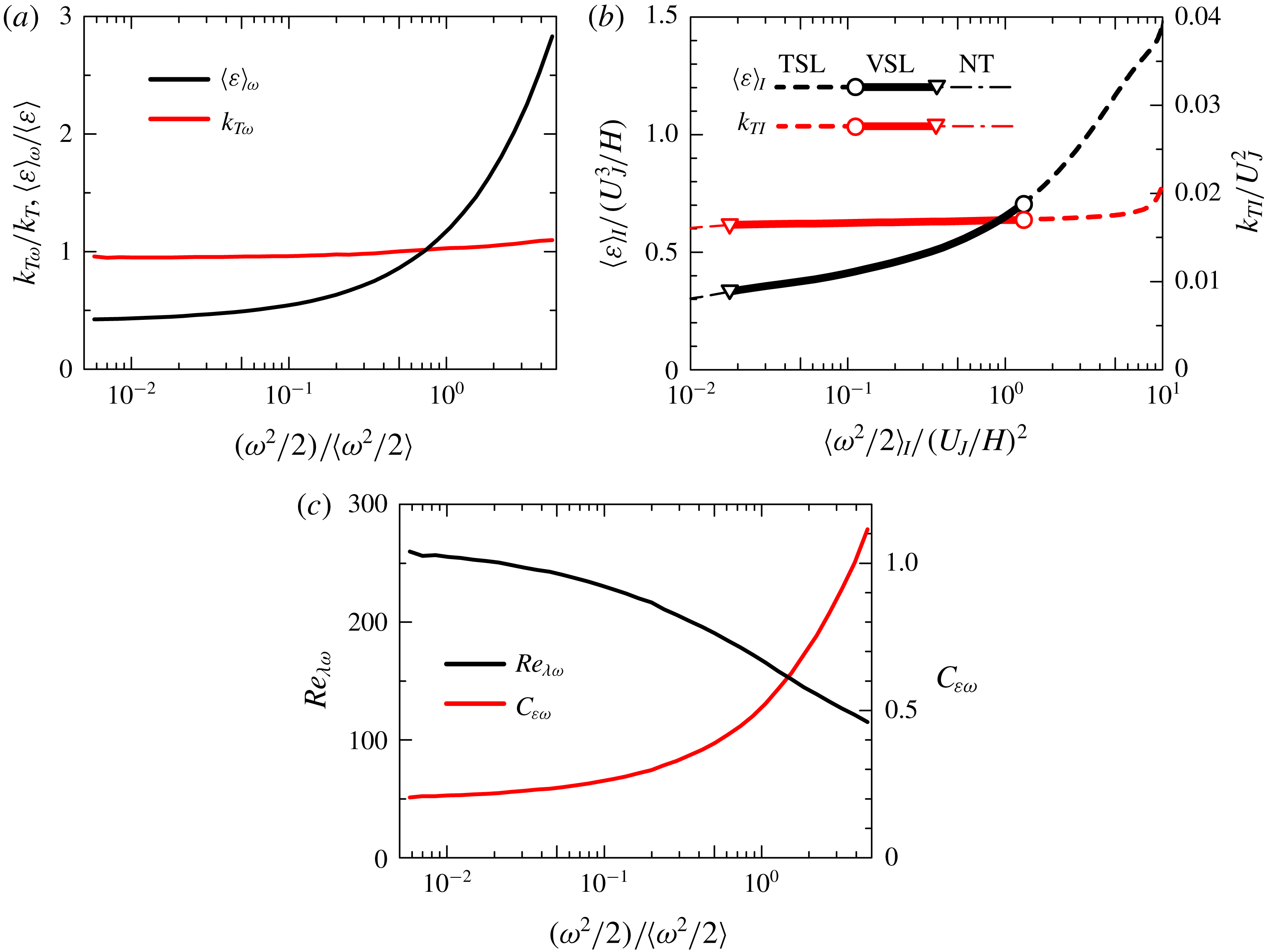
(a) Turbulent kinetic energy
 $k_{T\unicode[STIX]{x1D714}}=\langle u_{j}u_{j}\rangle _{\unicode[STIX]{x1D714}}/2$
and averaged kinetic energy dissipation rate
 $\langle \unicode[STIX]{x1D700}\rangle _{\unicode[STIX]{x1D714}}$
computed with averages conditioned on enstrophy in HIT1. (b) Turbulent kinetic energy
 $k_{TI}$
and averaged kinetic energy dissipation rate
 $\langle \unicode[STIX]{x1D700}\rangle _{I}$
plotted against
 $\langle \unicode[STIX]{x1D714}^{2}/2\rangle _{I}$
within the TNTI layer in PJET. Different lines are used for the non-turbulent region (NT), viscous superlayer (VSL) and turbulent sublayer (TSL) in (b). (c)
 $Re_{\unicode[STIX]{x1D706}}=(2k_{T\unicode[STIX]{x1D714}}/3)^{1/2}\unicode[STIX]{x1D706}_{\unicode[STIX]{x1D714}}/\unicode[STIX]{x1D708}$
and
 $C_{\unicode[STIX]{x1D700}\unicode[STIX]{x1D714}}=\langle \unicode[STIX]{x1D700}\rangle _{\unicode[STIX]{x1D714}}L/(2k_{T\unicode[STIX]{x1D714}}/3)^{3/2}$
computed with conditional averages on enstrophy for HIT1, where
 $\unicode[STIX]{x1D706}_{\unicode[STIX]{x1D714}}=(10\unicode[STIX]{x1D708}k_{T\unicode[STIX]{x1D714}}/\langle \unicode[STIX]{x1D700}\rangle _{\unicode[STIX]{x1D714}})^{1/2}$
.
Small-scale features of turbulent flows have been studied with the second and third invariants of velocity gradient tensor defined as
 $Q=(\unicode[STIX]{x1D714}_{i}\unicode[STIX]{x1D714}_{i}-2S_{ij}S_{ij})/4$
and
 $R=-(S_{ij}S_{jk}S_{ki}/3+\unicode[STIX]{x1D714}_{i}S_{ij}\unicode[STIX]{x1D714}_{j}/4)$
, respectively (Ooi et al.
Reference Ooi, Martin, Soria and Chong1999). Statistics of
 $Q$
and
 $R$
near the TNTI layer were presented in previous studies (da Silva & Pereira Reference da Silva and Pereira2008; Watanabe et al.
Reference Watanabe, Sakai, Nagata, Ito and Hayase2014; Vaghefi & Madnia Reference Vaghefi and Madnia2015; Mathew, Ghosh & Friedrich Reference Mathew, Ghosh and Friedrich2016; Watanabe et al.
Reference Watanabe, Jaulino, Taveira, da Silva, Nagata and Sakai2017a
). These studies showed that
 $\langle Q\rangle _{I}<0$
and
 $\langle R\rangle _{I}>0$
within the viscous superlayer, changing to
 $\langle Q\rangle _{I}>0$
and
 $\langle R\rangle _{I}<0$
in the turbulent sublayer. Figure 13(a) plots
 $\langle Q\rangle _{\unicode[STIX]{x1D714}}$
and
 $\langle R\rangle _{\unicode[STIX]{x1D714}}$
against
 $\unicode[STIX]{x1D714}^{2}/2$
for HIT1 while figure 13(b) plots
 $\langle Q\rangle _{I}$
and
 $\langle R\rangle _{I}$
against
 $\langle \unicode[STIX]{x1D714}^{2}/2\rangle _{I}$
near the TNTI layer for PJET. Figure 13(b) confirms these trends here for the planar jet while figure 13(a) displays similar features for the homogeneous isotropic turbulence. This has been explained by the presence of the vortices in the homogeneous isotropic turbulence and within the TNTI layers (Watanabe et al.
Reference Watanabe, Jaulino, Taveira, da Silva, Nagata and Sakai2017a
). In short
 $Q>0$
at the vortex cores and
 $Q<0$
surrounding these eddies (Davidson Reference Davidson2004).
Figure 14(a) shows the turbulent kinetic energy
 $k_{T\unicode[STIX]{x1D714}}=\langle u_{j}u_{j}\rangle _{\unicode[STIX]{x1D714}}/2$
and kinetic energy dissipation rate
 $\langle \unicode[STIX]{x1D700}\rangle _{\unicode[STIX]{x1D714}}$
, as a function of
 $\unicode[STIX]{x1D714}^{2}/2$
for HIT1 while figure 14(b) shows the results for PJET. In the two flow cases, both quantities increase with
 $\unicode[STIX]{x1D714}^{2}/2$
although the turbulent kinetic energy increases only slightly. Using the previous data for HIT1, the turbulent Reynolds number
 $Re_{\unicode[STIX]{x1D706}\unicode[STIX]{x1D714}}=(2k_{T\unicode[STIX]{x1D714}}/3)^{1/2}\unicode[STIX]{x1D706}_{\unicode[STIX]{x1D714}}/\unicode[STIX]{x1D708}$
and the non-dimensional dissipation rate
 $C_{\unicode[STIX]{x1D700}\unicode[STIX]{x1D714}}=\langle \unicode[STIX]{x1D700}\rangle _{\unicode[STIX]{x1D714}}L/(2k_{T\unicode[STIX]{x1D714}}/3)^{3/2}$
have been computed and shown in figure 14(c), where
 $\unicode[STIX]{x1D706}_{\unicode[STIX]{x1D714}}=\left(10\unicode[STIX]{x1D708}k_{T\unicode[STIX]{x1D714}}/\langle \unicode[STIX]{x1D700}\rangle _{\unicode[STIX]{x1D714}}\right)^{1/2}$
. Notice that the integral length scale
 $L$
is assumed to be independent of a local value
 $\unicode[STIX]{x1D714}^{2}/2$
since
 $L$
is computed from the auto-correlation function defined with two-point statistics. Similarly as in figure 8(c,d),
 $Re_{\unicode[STIX]{x1D706}\unicode[STIX]{x1D714}}$
decreases while
 $C_{\unicode[STIX]{x1D700}}$
increases with
 $\unicode[STIX]{x1D714}^{2}/2$
.
(a)
 $C_{\unicode[STIX]{x1D700}\unicode[STIX]{x1D714}}$
and (b)
 $C_{\unicode[STIX]{x1D700}\unicode[STIX]{x1D714}}Re_{\unicode[STIX]{x1D706}\unicode[STIX]{x1D714}}^{2}$
plotted against
 $Re_{\unicode[STIX]{x1D706}\unicode[STIX]{x1D714}}$
for HIT1.
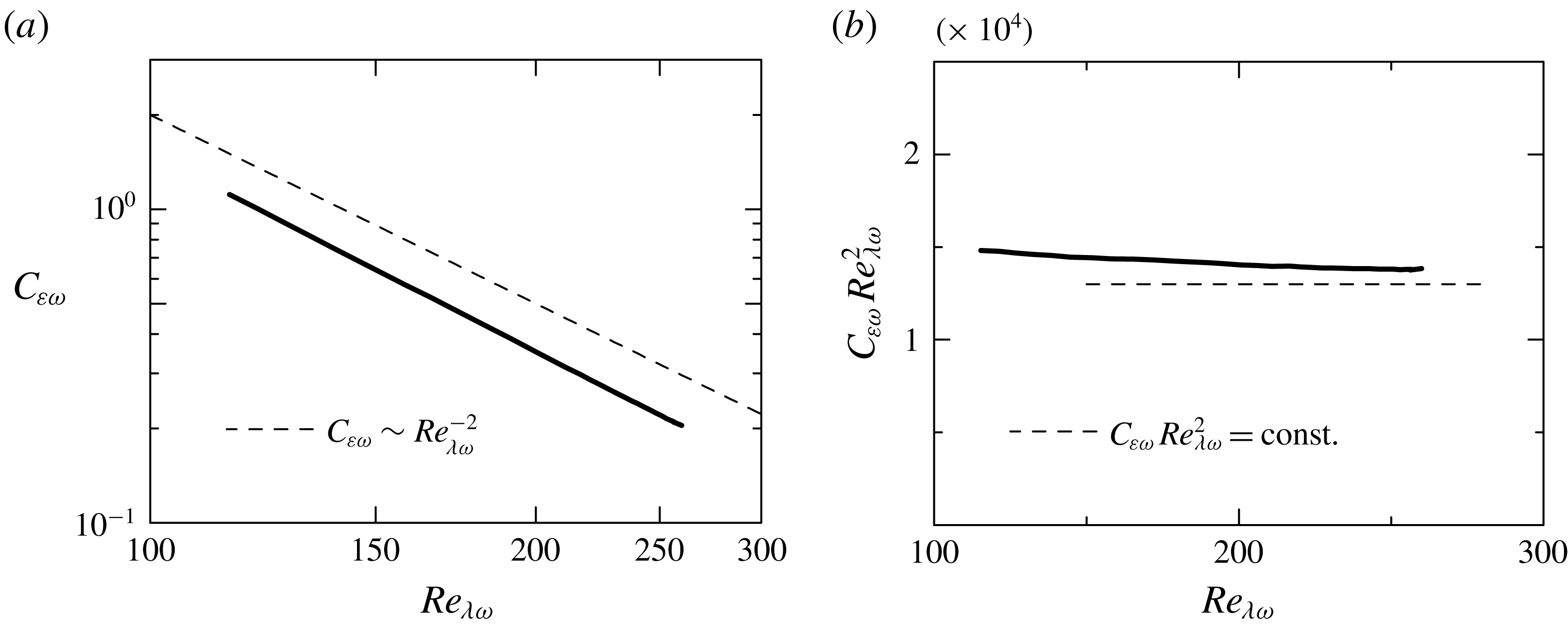
Figure 15(a,b) shows the dependency of
 $C_{\unicode[STIX]{x1D700}\unicode[STIX]{x1D714}}$
on
 $Re_{\unicode[STIX]{x1D706}\unicode[STIX]{x1D714}}$
for HIT1. It is clear that
 $C_{\unicode[STIX]{x1D700}\unicode[STIX]{x1D714}}\sim Re_{\unicode[STIX]{x1D706}\unicode[STIX]{x1D714}}^{-2}$
when the statistics are computed conditioned on enstrophy. This is particularly more so at higher
 $Re_{\unicode[STIX]{x1D706}\unicode[STIX]{x1D714}}$
i.e.
 $Re_{\unicode[STIX]{x1D706}\unicode[STIX]{x1D714}}\gtrsim 200$
since
 $C_{\unicode[STIX]{x1D700}\unicode[STIX]{x1D714}}Re_{\unicode[STIX]{x1D706}\unicode[STIX]{x1D714}}^{2}$
is relatively insensitive to
 $Re_{\unicode[STIX]{x1D706}\unicode[STIX]{x1D714}}$
(see figure 15
b). Because higher values of
 $Re_{\unicode[STIX]{x1D706}\unicode[STIX]{x1D714}}$
are associated with smaller values of
 $\unicode[STIX]{x1D714}^{2}/2$
(figure 14
c) we conclude that the relation
 $C_{\unicode[STIX]{x1D700}\unicode[STIX]{x1D714}}\sim Re_{\unicode[STIX]{x1D706}\unicode[STIX]{x1D714}}^{-2}$
arises in regions of relatively small local
 $\unicode[STIX]{x1D714}^{2}/2$
in HIT1. This reminds us of the same relation observed previously in the viscous superlayer and the beginning of the turbulent sublayer, where the mean enstrophy is also much smaller than in the turbulent core region (see figure 9). However, as remarked by an anonymous referee, it is not certain that
 $C_{\unicode[STIX]{x1D700}}\sim Re_{\unicode[STIX]{x1D706}}^{-2}$
can be explained in the same manner in the two situations.
Indeed, combining the definitions of
 $C_{\unicode[STIX]{x1D700}}$
,
 $Re_{\unicode[STIX]{x1D706}}$
and
 $\unicode[STIX]{x1D706}$
, one can write
 $C_{\unicode[STIX]{x1D700}}=15(L/\unicode[STIX]{x1D706})/Re_{\unicode[STIX]{x1D706}}=15(Re_{L}/Re_{\unicode[STIX]{x1D706}}^{2})$
, where
 $Re_{L}=u^{\prime }L/\unicode[STIX]{x1D708}$
. It follows that in HIT1, regions of roughly constant
 $u^{\prime }$
will display a trivial relation
 $C_{\unicode[STIX]{x1D700}}\sim Re_{\unicode[STIX]{x1D706}}^{-2}$
, since the integral scale
 $L$
is constant. It is clear that the local variations of
 $Re_{\unicode[STIX]{x1D706}}$
at these locations must come from local variations of
 $\unicode[STIX]{x1D700}$
(and
 $\unicode[STIX]{x1D714}^{2}/2$
). Also, from the previous figures and discussion it is clear that in these regions both
 $\unicode[STIX]{x1D700}$
and
 $\unicode[STIX]{x1D714}^{2}/2$
is very small, but
 $Re_{\unicode[STIX]{x1D706}}$
is high. Thus, one concludes that
 $C_{\unicode[STIX]{x1D700}}\sim Re_{\unicode[STIX]{x1D706}}^{-2}$
is observed in the homogeneous isotropic turbulence in regions of high
 $Re_{\unicode[STIX]{x1D706}}$
, where
 $u^{\prime }$
is roughly constant and where
 $\unicode[STIX]{x1D714}^{2}/2$
(and
 $\unicode[STIX]{x1D700}$
) are very small. This suggests that this relation is connected to the somehow ‘void’ regions between the eddies, or between the large clusters of eddies existing in the homogeneous isotropic turbulence. The relation
 $C_{\unicode[STIX]{x1D700}}\sim Re_{\unicode[STIX]{x1D706}}^{-2}$
observed in the viscous superlayer and a part of the turbulent sublayer certainly arises in a region where the level of
 $\unicode[STIX]{x1D700}$
and
 $\unicode[STIX]{x1D714}^{2}/2$
is very small (see figure 8
a), and furthermore, no vortices are to be found inside these regions (which are bounded by the eddies).



