1. Introduction
Simultaneous localization and mapping (SLAM) is a technique used by mobile robots equipped with sensors to estimate their motion state and incrementally build a map of the surrounding environment without prior knowledge [Reference Durrant-Whyte and Bailey1]. SLAM was initially proposed by Smith and Cheeseman [Reference Smith, Self and Cheeseman2] in 1988 and has been further improved by researchers such as Leonard and Durrant-Whyte [Reference Leonard and Durrant-Whyte3]. It has become a cornerstone of mobile robot technology and finds widespread applications in autonomous intelligent driving [Reference Zhang, Zhao and An4, Reference Liu, Di and Xu5], unmanned aerial vehicles (UAVs) [Reference Elmokadem and Savkin6], autonomous underwater vehicles (AUVs) [Reference Palomeras, Carreras and Andrade-Cetto7, Reference Zhang, Zhao and An8], three-dimensional reconstruction [Reference Wang, Zhang and Song9], etc. SLAM is one of the most extensively studied topics in mobile robotics.
The early SLAM algorithms relied mainly on sonar sensors, but their performance was unsatisfactory. Currently, the main sensors used in SLAM for mobile robots include odometry, LiDAR, and depth cameras. Based on the primary sensors used in modern SLAM algorithms, SLAM can be divided into two categories: visual SLAM and LiDAR SLAM. Visual SLAM usually utilizes cameras, which have lower costs and provide rich information. However, it is prone to errors due to lighting variations and fast motion, leading to blurred images [Reference Wang and Zhang10], making it challenging to directly construct two-dimensional grid maps suitable for localization and navigation [Reference Yi and Shen11]. LiDAR SLAM relies predominantly on LiDAR sensors due to their exceptional detection accuracy and high-resolution data. One key advantage of LiDAR is its immunity to lighting conditions, allowing it to capture reliable scan data consistently.
Currently, research on single-robot SLAM has reached a mature stage [Reference Hu, Zhou and Miao12]. However, when it comes to complex tasks and large-scale environments, using a single robot alone poses challenges such as low work efficiency, poor stability, and low map accuracy. Compared with single-robot SLAM, multi-robot SLAM considers the process of multiple robots simultaneously positioning and mapping in the same environment. Collaborative SLAM (CSLAM) is a specific implementation of multi-robot SLAM, which emphasizes information sharing and fusion between robots to achieve collaborative mapping, especially when global optimization is required. It offers advantages such as high efficiency, robustness, and improved map accuracy, making it more suitable for large-scale or sparse environments [Reference Choi and Lee13]. However, extending single-robot SLAM to multi-robot SLAM introduces new challenges. These include communication issues between multiple robots [Reference Liu14], efficient frontier detection, collaborative planning [Reference Dubois, Eudes and Frémont15] and task allocation for robot groups, and concerns regarding the accuracy and efficiency of global fusion when integrating locally constructed maps from individual robots [Reference Li, He, Zhang and Zhang16].
So far, there have been many surveys and reviews on SLAM and CSLAM. Many of the existing surveys focus on visual SLAM methods [Reference Zou, Tan and Yu17–Reference Zheng, Su and Lin20]. Huang et al. [Reference Huang21] and Xu et al. [Reference Xu, Zhang and Yang22] summarized the common LiDAR SLAM frameworks and core module functions and studied multi-sensor fusion technology, but provided inefficient literature reviews and were limited to single-robot LiDAR SLAM. Yue et al. [Reference Yue, Zhang, Chen, Chen, Zhou and He23] summarized three different types and configurations of LiDAR, but discussed the issues of multi-robot LiDAR systems less. Rizk et al. [Reference Rizk, Awad and Tunstel24] focus on robot agents and emphasize the challenges in the MRS sub-fields, including task decomposition, coalition formation, task allocation, perception, and multi-agent planning and control. Their work was an excellent and worthwhile review but lacked an in-depth analysis of LiDAR sensors. Refs. [Reference Zhao, Shao, Wang, Fang, Zhang and Zhao25, Reference Aloui, Guizani, Hammadi, Haddar and Soriano26] reviewed and analyzed the key issues and current challenges in CSLAM, but provided insufficient literature reviews and limited reference for LiDAR SLAM.
Lajoie et al. [Reference Lajoie, Ramtoula, Wu and Beltrame27] provided a complete overview of the CSLAM research landscape, detailing the overall framework, popular algorithms, opening issues, and ongoing development trends of CSLAM. However, they haven’t mentioned the analysis of LiDAR SLAM exploration, planning, and mapping issues. Zhang et al. [Reference Zhang, Shi and Li28] conducted a comprehensive review of the scientific connotation, key difficulties, research status, and future development trends of 3D LiDAR but did not consider the task challenges encountered in practical SLAM applications, such as map fusion. Zhang et al. [Reference Zhang, Shi and Li29] conducted a comprehensive review of the location recognition SLAM methods and related research using LiDAR sensors but only focused on one module of LiDAR scanning. Chen [Reference Chen, Wang, Gao, Shang, Zhou, Li, Xu and Hu30] reviewed multi-robot collaborative SLAM from the perspective of multimodal data fusion and discussed existing algorithms from the perspective of machine learning classification.
Different from prior research, our review focuses on the literature on multi-robot cooperative SLAM framework based on LiDAR. Figure 1 shows the overall framework of this study. The main contributions are as follows:
-
• Key SLAM Techniques: It discusses the theoretical basis of LiDAR SLAM technology, SLAM front-end and back-end, and popular 2D/3D LiDAR SLAM algorithms.
-
• Multi-robot LiDAR CSLAM Systems: This paper reviews CSLAM in detail, including the most advanced CSLAM systems and the framework of CSLAM systems, and analyzes the core issues of CSLAM such as data association, loop closure detection, and global optimization.
-
• Challenges of MRS Sub-fields: The study decomposes the multi-robot LiDAR SLAM system into three core sub-fields: frontier detection, task allocation, and map fusion. This paper provides a comparative analysis of the algorithms addressing these issues.
-
• Open Challenges and Trends: Finally, the paper discusses the development challenges and emerging trends in LiDAR SLAM, offering insights into future research directions.
Multi-robot LiDAR SLAM structure diagram.

This study provides a valuable reference for researchers aiming to understand various LiDAR SLAM applications. The paper is organized as follows. The theoretical foundations of LiDAR SLAM are briefly reviewed in Section 2. Section 3 focuses on analyzing the system framework of CSLAM, including the system form and key challenges of CSLAM. Then, Section 4 reviews three subfields of multi-robot LiDAR systems: frontier detection, task allocation, and map fusion, as well as existing methods to address these challenges. Therefore, in Section 5, several open challenges and future development trends of multi-robot LiDAR SLAM are pointed out. Finally, this paper summarizes the conclusions in Section 6.
2. Key SLAM techniques
Before formally introducing the LiDAR SLAM system, we first review the relevant knowledge of building the LiDAR SLAM system model to provide some reference for beginners.
2.1. Kinematic model of mobile robot
The kinematic model of a mobile robot is the basis for estimating the robot’s posture. Mobile robot systems commonly employ Cartesian coordinate systems and polar coordinate systems to represent the relative positions of robots and obstacles [Reference Zhu31]. When calculating the robot’s position and orientation, the Cartesian coordinate system is simpler and more intuitive. Therefore, the model construction in this chapter adopts the Cartesian coordinate system.
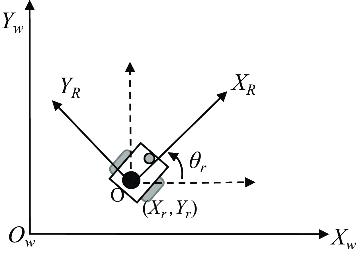
Figure 2 depicts the coordinate system utilized by the mobile robot. The world coordinate system, denoted as
 $XwOwYw$
, acts as a reference frame for measuring the displacement of all objects within the system. In the world coordinate system, the robot’s pose at time
 $k$
is
 $X_k =(x_r,y_r,\theta _r)$
. Let the robot coordinate system be
 $XrOrYr$
. This coordinate system moves with the movement of the robot. The coordinate of its origin in the world coordinate system represents the robot’s pose, and the angle between the horizontal axis and the horizontal axis of the world coordinate system represents the posture of the robot [Reference Zhao32].
Mobile robot coordinate system.

If a point
 $X_0= [x_0, y_0]^{T}$
in the robot coordinate system, then the coordinates of this point
 $X_{w}^{0}= [x_{w}^{0}, y_{w}^{0}]^{T}$
in the world coordinate system can be obtained by (1):
 \begin{equation} \left \{\begin{array}{l} x_{W}^{0}=x_{r}+x_{0} \cos \theta _{r}-y_{0} \sin \theta _{r} \\[3pt] y_{W}^{0}=y_{r}+x_{0} \sin \theta _{r}+y_{0} \cos \theta _{r} \end{array}\right . \end{equation}
The motion of a mobile robot occurs in a three-dimensional environment, with the coordinate system centered at the robot’s chassis center point. The
 $X$
-axis represents the forward direction, the
 $Y$
-axis is perpendicular to the forward direction, and the
 $Z$
-axis passes through the center of the chassis and is perpendicular to the robot’s base. Simultaneously, it is necessary to simplify the robot model appropriately by considering the robot’s motion in a two-dimensional plane. Therefore, the three-dimensional coordinate system can be simplified to a two-dimensional
 $XOY$
coordinate system, and the robot’s pose representation consists of the two-dimensional plane coordinates and the steering angle.
Due to its simple structure and easy control, the two-wheel differential motion structure is widely used in wheeled mobile robots. The robot moves in a circular arc around a certain center, as shown in Figure 3.
Mobile robot kinematic model.

The calculation formulas for angular velocity and linear velocity are as follows:
 $$\begin{align}\omega &= \frac {v_{R}-v_{L}}{2d}\end{align}$$
 $$\begin{align}v &= \frac {v_{R}+v_{L}}{2}\end{align}$$
Where
 $v$
and
 $\omega$
represent the linear velocity and angular velocity of the robot during movement,
 $v_L$
and
 $v_R$
are the linear velocities of the left and right wheels, and
 $\omega _L$
and
 $\omega _R$
are the angular velocities of the left and right wheels, respectively.
 $r$
represents the radius of rotation around the center of the circle, and the distance between the two wheels is 2
 $d$
.
From the above formula (3), we can get that in the kinematic model of the mobile robot, the linear velocity and angular velocity of the robot’s motion are only related to the linear velocity of the robot’s left and right wheels, and the wheel spacing. And half of the wheel spacing
 $d$
is a constant, which has been set when the robot leaves the factory. Therefore, the robot’s motion can be calculated by measuring
 $v_L$
and
 $v_R$
through the encoders on the wheels.
Mobile robot odometer linear model and odometer arc model.

2.2. Sensor model
2.2.1. Odometer model
The odometer calculates the distance traveled by the mobile robot per unit of time by using the pulse data output by the photoelectric encoder within a certain period to estimate the robot’s movement over time. The odometer can mitigate many errors arising from uncertainties in the robot’s navigation process and enhance the accuracy of map construction. The two-wheel differential chassis has a simple structure, low cost, and a relatively simple model to establish, so it is used in various types of robot production [Reference Hang33]. Figure 4 shows two models of odometer: the straight line model and the arc model.
-
• Straight Line Model. The motion of the robot is continuous, but it is usually considered to be discrete in time to simplify the calculation process [Reference Zhou34]. The straight line model is represented in Figure 4(a). We can know that the dead reckoning Eq. (4) for the robot’s linear motion is:
(4) \begin{equation} \left \{\begin{array}{c} x_{k+1}=x_{k}+\Delta S_{k} \cos \theta _{k} \\[2pt] y_{k+1}=y_{k}+\Delta S_{k} \sin \theta _{k} \\[2pt] \theta _{k+1}=\theta _{k}+\Delta \theta _{k} \end{array}\right . \end{equation}
Where
$(x_k,y_k, \theta _k)$
represents the robot coordinates,
$\Delta S_k$
,
$\Delta \theta _k$
represents the robot’s linear motion distance and rotation angle. Substituting the angular velocity and linear velocity
$\omega$
,
$v$
of the robot’s motion, the robot’s posture at the next moment is:(5)
\begin{equation} \left \{\begin{array}{c} x_{k+1}=x_{k}+v \Delta t \cos \theta _{k} \\[2pt] y_{k+1}=y_{k}+v \Delta t \sin \theta _{k} \\[2pt] \theta _{k+1}=\theta _{k}+\omega \Delta t \end{array}\right . \end{equation}
-
• Arc model. The robot rotates around a point in an arc and moves to the next position. This model considers both the movement of the robot and the change of the direction angle [Reference Qin35], which is shown in Figure 4(b). The dead reckoning equation for the robot’s circular motion is (6):
(6)
\begin{equation} \left \{\begin{array}{c} x_{k+1}=x_k+D\cos \left (\theta _k+\frac {\alpha }{2}\right )\\[2pt] y_{k+1}=y_k+D\sin \left (\theta _k+\frac {\alpha }{2}\right )\\[2pt] \theta _{k+1}=\theta _k+\alpha \end{array}\right . \end{equation}
Where
$\alpha$
represents the angle that the robot rotates in time
$\Delta t$
and S represents the arc of rotation, which is approximately the displacement
$D$
between two points. Substituting the angular velocity
$\omega$
and linear velocity
$v$
into the robot’s motion equation, the robot’s posture changes to:(7)
\begin{equation} \left \{\begin{array}{c} x_{k+1}=x_k+v\Delta t\cos \left (\theta _k+\frac {\omega \Delta t}{2}\right )\\[2pt] y_{k+1}=y_k+v\Delta t\sin \left (\theta _k+\frac {\omega \Delta t}{2}\right )\\[2pt] \theta _{k+1}=\theta _k+\omega \Delta t \end{array}\right . \end{equation}
Based on the formula (7) provided above, the future posture of the robot can be calculated by considering its current posture, velocity, and elapsed time.


2.2.2. IMU model
An inertial measurement unit (IMU) is a precision sensor module consisting of an accelerometer and a gyroscope that is used to capture inertial data, including the linear acceleration and angular velocity of an object. This technology is widely used in various fields such as aerospace engineering, robotic systems, and automotive navigation. In contemporary SLAM systems, the integration of LiDAR and IMU technology is becoming more and more common [Reference Li, Wang and Li36–Reference Zhang39].
Using the measurement data and kinematic equations of the IMU, the position and attitude of the robot can be determined. However, there are noise and drift errors when the robot moves, and the raw data often leads to inaccurate pose estimates. The measurement formulas of the angular velocity Wt and linear velocity at of the IMU are as follows:
 \begin{align} \hat {a_{t}} &=R_{t}^{BW}(a_t + g)+{b}_{a}+n_{t}^{a} \\[-28pt] \nonumber \end{align}
 \begin{align} \hat {w_{t}} &=w_{t}+b_{g}+n_{t}^{g} \end{align}
Where
 $n_{t}^{a}$
and
 $n_{t}^{g}$
represent the measurement noise of the accelerometer and gyroscope at time
 $t$
, respectively,
 $b_{a}$
and
 $b_{g}$
represent the deviations of the accelerometer and gyroscope, respectively, which can be considered as constant deviations in a short period of time.
 $g$
represents the gravitational acceleration of the current coordinate system,
 $R_{t}^{BW}$
indicates the attitude of system
 $B$
relative to system
 $W$
at the
 $t$
moment.
IMU error models can be categorized into two primary types: deterministic errors and stochastic errors during operation. Deterministic errors, including bias and scale factor, can be effectively compensated through pre-calibration procedures. In contrast, stochastic errors are typically modeled under the assumption of Gaussian distribution characteristics, encompassing phenomena such as Gaussian white noise and biased random walk [Reference Brossard and Bonnabel40]. From a performance perspective, IMUs can be classified into three distinct tiers: (1) high-precision marine and aerospace-grade inertial navigation systems, which are characterized by their large size, exceptional accuracy, and substantial cost; (2) tactical and industrial-grade inertial sensors, which offer significant application value and are widely employed in scenarios requiring high-performance measurements at relatively moderate costs, such as in delivery robots and UAVs; (3) consumer-grade sensors designed for mass-market applications, prioritizing cost-effectiveness over precision.
2.2.3. LiDAR model
In mobile robot SLAM, the availability of accurate and reliable sensor data is crucial for constructing precise maps. Various sensors are commonly employed, including IMU, wheel encoders, sonar, LiDAR, and depth cameras [Reference Wei41]. Distance sensors like sonar and LiDAR actively detect objects by transmitting and receiving signals, allowing for effective measurement of the distance between the robot and obstacles. However, sonar sensors are susceptible to environmental noise, which can introduce disturbances into the data readings. On the other hand, visual sensors such as depth cameras are significantly influenced by ambient light conditions, posing challenges for their operation in both dimly and brightly lit environments.
LiDAR uses the time difference between the laser beam emitted and the laser reflected by the obstacle to calculate the distance between the obstacle and itself. The collected object information presents a series of scattered points with accurate angle and distance information, which is called a point cloud. Compared with other sensors, LiDAR has the characteristics of high accuracy, fast solution speed, and no restrictions on light environment. It finds extensive applications in autonomous driving, mapping, positioning, and navigation domains [Reference Yoneda, Tehrani, Ogawa, Hukuyama and Mita42]. Figure 5 is divided into the device appearance of the laser (a) and the scanning model (b).
Appearance and scanning model of LiDAR.

There are two main types of LiDAR ranging models: triangulation and ToF (Time of Flight). Triangulation obtains distance information by solving triangles based on the camera’s spot imaging position, while ToF calculates distance based on the measured light’s flight time, which has a higher accuracy [Reference Lu43].
Two model of LiDAR: triangulation and ToF.

In the triangulation distance measurement of Figure 6(a), the distance to the object is proportional to the angle of the reflected light. The concept of the triangle equation can be used to estimate the actual distance [Reference Wang44]. There is a distance s between the transmitter and the center o of the receiver of the LiDAR using the triangulation distance measurement method, which is called the baseline. The distance from the object to the baseline is q. The transmitter emits a laser beam at a certain angle
 $\beta$
, which hits an object at a distance d and is received by the receiver after reflection. The focal length of the receiver is f, and the distance from the receiving point to the center o of the receiver is x. The LiDAR measures the distance d of an object using the triangulation formula, as depicted in calculation formula (10).
 \begin{equation} d=\frac {fs}{2x\sin {\beta }} \end{equation}
Figure 6 (b) shows the working principle of ToF ranging. A high-frequency laser beam of a specific power is emitted to the target object, and the laser signal reflected to the receiver is processed with the emission signal. The target position information is obtained by calculating the product of the time difference between the emitted laser and the reflected laser and the speed of light [Reference Zheng45]. Compared with triangulation-ranging LiDAR, ToF LiDAR has higher accuracy and stability. ToF calculates the distance d to the object based on the light flight time. The calculation formula is shown in (11). Where d is the distance to the object, c is the speed of light,
 $\Delta t$
is the time difference between the laser emission and reception, and n is the average reflectivity of the transmission medium.
 \begin{equation} d=\frac {c \Delta t}{2n} \end{equation}
2.3. Map representation
After obtaining data through sensors such as LiDAR, the raw data needs to be converted into a visual data representation, namely a map representation, which is a structure used to store and express environmental information. Commonly used map representation methods can be roughly divided into three types: metric map, topological map, and metric semantic map. Each map representation method has its advantages and disadvantages. The following is a brief introduction to these different map types.
2.3.1. Metric map
Metric maps are the most commonly used map representations in SLAM, with real physical dimensions. Typical representatives include the Occupancy grid Map, Point cloud Map, and Feature Map [Reference Moravec46]. The point cloud map [Reference Kim, Chen and Cho47] is shown in Figure 7(a). The map created using the LiDAR sensor is represented as a grid map, as shown in Figure 7(b). The occupation grid map was first proposed by Elfs [Reference Elfes48] and Morave [Reference Moravec46] in the late 1980s, and its basic idea is to use different pixel values to represent the occupation state of the corresponding area, that is, the existence of obstacles.
In general, a two-dimensional raster map represents a specific height slice of information within a three-dimensional space in a particular state. The grid cells in a raster map can be categorized into three states: occupied, vacant, and unknown. Raster maps provide comprehensive spatial distribution and scale information, serving as the foundation for multi-robot exploration map fusion and finding applications in various SLAM frameworks [Reference Cai, Kong, Ren, Zhu, Lin and Zhang49]. A feature map is an environmental map constructed by a robot to extract distinctive features from the surrounding environment. It is primarily employed in indoor scenarios, utilizing geometrically prominent elements such as tables, chairs, doors, and windows to represent the environment. Scale maps find primary applications in map construction, localization, and small-scale path planning tasks.
Representation of 3D point cloud map (a), occupancy grid map (b), and topological map (c).

2.3.2. Topological map
Topological maps are widely used in SLAM, consisting of nodes and edges that represent the connected relationships between different locations. Unlike physical maps, topological maps lack real-world dimensions and focus solely on spatial connections. The structure of a topological map, as depicted in Figure 7(c) [Reference Shienman, Kitanov and Indelman50], simplifies the requirement for precise details, resulting in a more compact representation. The benefits of topological maps include high efficiency in autonomous routing, fast data processing, and reduced memory consumption for mobile robots. Consequently, they are frequently employed in large-scale robot path planning.
2.3.3. Metric-semantic map
Metric-semantic map is a map representation method combined with SLAM and deep learning that correlates semantic information with traditional metric maps [Reference Wang, Shang and Gao51]. It adds labels based on scale maps and is often used for human-computer interaction [Reference Bao, Pan, Yang and Huan52] to capture the state and shape of objects in the environment for description and to build environmental maps. Qin [Reference Qin, Zheng, Chen, Chen and Su53] proposed a lightweight positioning scheme that relied on low-cost cameras and compact visual semantic maps, and its semantic elements included lane lines and walkways. The metric semantic map has become one of the development prospects of SLAM research in the future.
Different maps have advantages and disadvantages, so using a combination of maps is an optional solution. Zhang et al. [Reference Zhang, Tian, Shao, Liu, Zhang and Duan54] constructed a metric semantic map, which removes unrelated redundant points compared with traditional maps and is convenient for robots to locate targets, which is suitable for object search. Kuang et al. [Reference Kuang, Li and Zhang55] improved the initial particle swarm distribution in the global positioning of the adaptive Monte Carlo localization algorithm based on the semantic grid map. The semantic grid map solved the problem of environmental information degradation caused by 2D LiDAR and improved the robot’s perception of the environment.
2.4. LiDAR SLAM framework
In an unknown environment, the problem of SLAM can be defined as follows: the mobile robot relies exclusively on its onboard sensors to achieve self-localization while concurrently constructing a map of the environment. The self-localization of the robot (pose estimation) and the construction of the unknown environment map are mutually dependent. Assuming that the mobile robot is equipped with sensors and is navigating within the unknown environment, and taking into consideration that the sensor measurements are discrete due to sampling at discrete time intervals, the robot’s motion can be mathematically described using discrete time steps, denoted as
 $t = 1,\ldots , T$
. The sensors integrated into the robot’s system include LiDAR, odometry, and IMU. The relationship between the robot’s sensor measurements and its motion can be expressed using motion (12):
 \begin{equation} x_{T}=f\left (x_{T-1}, u_{T}, w_{T}\right ) \end{equation}
Among them,
 $x_T$
represents the position of the mobile robot at a certain moment, the random variable sequence
 $x_{1:T} = \{x_1, \ldots , x_T\}$
is the motion trajectory of the mobile robot in an unknown environment;
 $u_T$
represents the reading of the motion sensor it carries, such as acceleration, angular velocity, and other parameters;
 $w_T$
represents the motion noise in the process, that is, the deviation between the actual motion process and the issued motion command.
The map constructed by the mobile robot is composed of different landmarks.
 $z_{T,j}$
is the observation data generated by the mobile robot observing the landmark
 $y_j$
through the sensors it carries at the location
 $x_T$
. The process is described by an abstract function
 $h$
. The noise in the observation process is
 $v_{T, j}$
, then the observation (13) can be obtained:
 \begin{equation} z_{T,j}=h\left (y_{j}, x_{T}, v_{T, j}\right ) \end{equation}
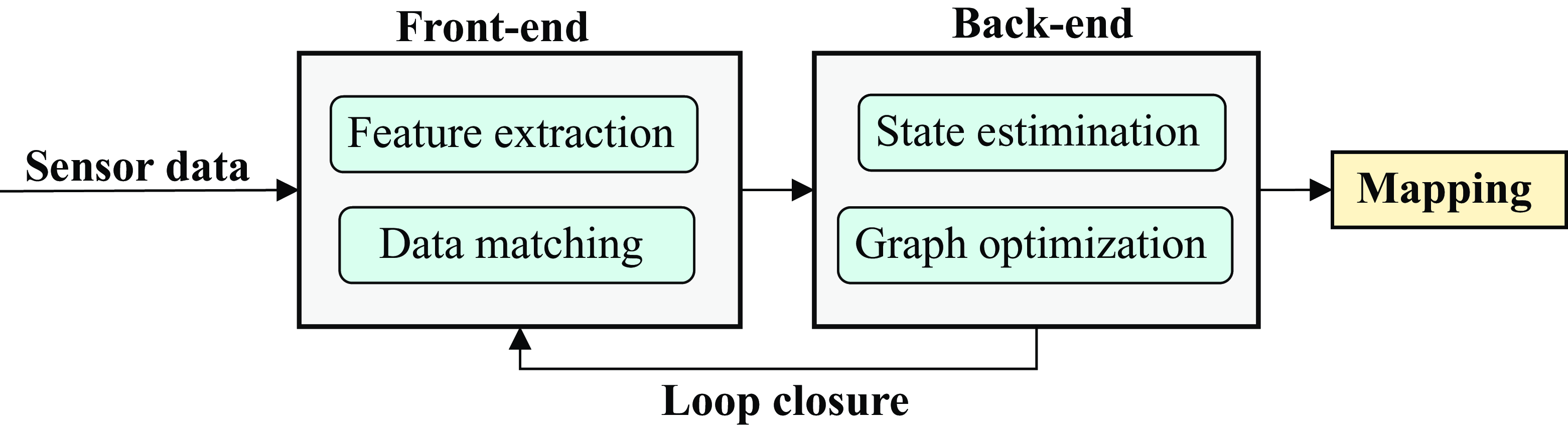
Single-robot SLAM is the basis of the multi-robot SLAM. Figure 8 provides a common framework of single robot LiDAR SLAM framework, which includes two components: front-end and back-end [Reference Wu56]. Sensor data mainly comes from LiDAR and wheel odometers. The LiDAR obtains environmental information through laser scanning. The wheel odometer continuously obtains the robot’s mileage information through the encoder of the mobile chassis [Reference Song57]. The SLAM front-end collects data through scanning measurement, and the back-end performs state estimation and map optimization.
Single-robot LiDAR SLAM framework.

2.4.1. SLAM front-end
Front-end matching is a common data association method in LiDAR SLAM, where a mobile device reads a previous position and uses the current position to measure the relationships between neighboring devices.
The accuracy and computational efficiency of the scan matching algorithm directly affect the accuracy of SLAM algorithm position estimation and map construction, as well as providing back-end optimization capabilities. Theoretically, it can be divided into iterative closest point (ICP)-based scanning, feature-based scanning, mathematical property-based scanning, correlation-based scanning, optimization-based scanning [Reference Liang, Cao, Wang and Yu58], etc.
The iterative closest point algorithm was proposed by Besl [Reference Besl and McKay59] and Chen [Reference Chen and Medioni60] in 1992. The essence of scanning matching is to calculate the translation matrix and rotation matrix with the smallest Euclidean distance between the corresponding point pairs between two point cloud frames and then use this translation matrix and rotation matrix as the pose change relationship between the two point cloud frames to be matched through iteration [Reference Qi61]. However, this algorithm is prone to fall into local optimality. In the improved algorithm for solving the optimal pose, Low [Reference Low62] and others proposed an improved solution to expand the distance from point to point to point to line or even point to surface [Reference Phillips, Liu and Tomasi63]. In addition, Nicolai [Reference Nicolai, Skeele, Eriksen and Hollinger64] and others combined the three-dimensional point cloud with the CNN network for training, which improved the real-time performance.
The feature-based scan matching algorithm removes key elements from the laser scan data through matching, such as point, line, surface, and other set primitives or combinations, features such as curvature and normal vector, and some custom feature descriptors to achieve fast correspondence matching. It can solve the pose change without providing initial values. Zhang [Reference Zhang and Singh65] proposed feature points for scan matching using point-to-boundary and point-to-plane methods, and the effect of the LiDAR odometer is relatively accurate.
The mathematical property-based scan matching algorithm converts the point cloud registration problem into a mathematical formulation. A notable example of such an algorithm is the distribution-based Normal Distribution Transform (NDT) [Reference Chiang, Chiu, Srinara and Tsai66]. NDT is a mathematical point cloud registration algorithm that utilizes Gaussian distribution to model the captured point cloud data [Reference Liu, Xu, Tang, Qian and Geng67]. Compared with ICP and feature-based algorithms, NDT exhibits fast speed, short calculation time, and the ability to compensate for a wider range of initial poses [Reference Magnusson68].
The correlation scan matching method (CSM) conducts point cloud matching utilizing a probabilistic grid map. Each grid retains a logarithmic probability of occupancy. In the case of a new laser scan frame, all point estimations are projected onto the grid map. The current pose score, which represents the credibility of the pose, is determined by summing the logarithmic probabilities of the grid occupied by the laser. Nevertheless, the brute force matching approach is slow, leading to the proposal of a branch and bound acceleration method that subdivides the environmental resolution to compute the optimal pose. Du et al. [Reference Du, Chen and Lou69] proposed a localization method for indoor mobile robots based on the CSM technique, which uses 2D LiDAR to provide accurate and fast pose estimation based on a public space map.
The optimization-based scan matching method is essentially a gradient-based method and solution. Hector-SLAM and Cartographer are two representative optimization-based algorithms, among which Hector-SLAM is a pure map optimization method, while Cartographer is an optimization method that combines CSM and gradient optimization.
2.4.2. SLAM back-end
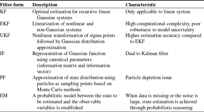
Back-end optimization is an effective method to reduce the accumulated local errors in front-end matching. In principle, it can be mainly divided into filtering-based optimization methods and graph optimization-based methods [Reference Tee and Han70]. For filtering-based LiDAR SLAM, the front-end estimates the pose of the mobile robot through point cloud data registration, and the back-end optimizes the pose calculated by the front-end using filtering theory [Reference Grooms71]. Representative filtering methods include the Kalman filter (KF), extended KF (EKF), unscented KF (UKF), information filter (IF), Particle Filter (PF), and expectation maximization. The filter forms are shown in Table I.
Filter forms.

The more classic one is the EKF method, which solves the problem of nonlinear non-Gaussian application scenarios and has been applied to LiDAR CLSAM. The EKF-based SLAM algorithm will initialize the map, update the current robot posture and state according to the odometer data and kinematic model, initialize the road sign, correct the current state through the road sign, and update the new roadside information. The disadvantage of the EKF method is that it needs to store the mean and variance of all states, and the computational complexity is high. The UKF method is a combination of the unscented transform (UT) and the standard KF system, using UT to handle the nonlinear transfer of the mean and covariance. The PF method uses the recursive filter of the Monte Carlo method to generate particles, uses the system model to predict the state, updates the particle weights, resamples and discards particles with smaller weights, and finally calculates the estimated value of the state variable. The IF method uses the information matrix to represent and update the state estimate and its uncertainty.
Compared to filtering-based SLAM solutions, graph optimization-based approaches can effectively adapt to larger and more complex scenarios. Graph optimization involves expressing a conventional optimization problem in the form of a graph theory, where the robot’s posture is represented as a node and the relationships between postures form the edges. Once these nodes and edges are established, the robot’s posture is adjusted to satisfy the imposed constraints [Reference Fang, Panah, Masoudi, Barzegar and Fatehi72]. Factor graph optimization is a specific method within graph optimization that partitions the graph into variable nodes and factor nodes. In the case of a long path, check whether it has returned to the previous position. If a closed loop is detected, add corresponding constraints to improve the global consistency of the map. After the optimization is completed, update the robot’s posture and the position of the map features.
In an unknown environment, for a highly uncertain robot, it is worth considering whether to continue exploring the unknown area or revisit the already explored region after completing exploration in a partial area. This situation poses the “exploration-exploitation dilemma” in frontier detection. Grabowski [Reference Grabowski, Khosla and Choset73] observed that regions of interest where sensor readings overlap may provide more informative data than unexplored areas. In the SLAM mapping process, the front-end odometry only considers keyframes from adjacent periods, leading to the accumulation of errors over time and resulting in unreliable long-term estimation results. Loop closure is employed to detect potential loops based on the constraint relationship between point cloud data frames. By correcting drift errors, globally consistent trajectories, and maps are constructed, enabling global optimization. From an algorithmic perspective, loop closure can be broadly categorized as scan-to-scan, scan-to-map, or map-to-map loop closure.
2.5. LiDAR SLAM algorithms
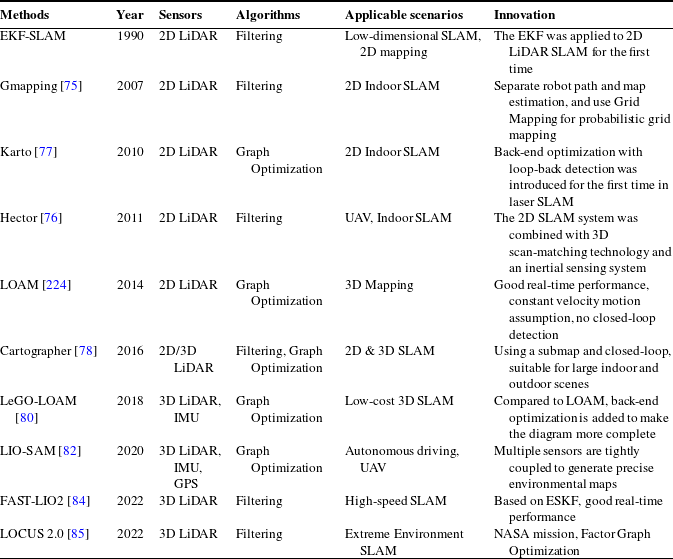
The LiDAR-centric solution is one of the mainstream solutions for SLAM [Reference Ebadi, Bernreiter and Biggie74]. According to the number of laser beams in a LiDAR sensor, it can be divided into single-line LiDAR (2D LiDAR) and multi-line LiDAR (3D LiDAR). In this section, we will conduct a comprehensive literature review on two LiDAR SLAM algorithms: (1) 2D LiDAR SLAM, and (2) 3D LiDAR SLAM. Table II summarized classical LiDAR SLAM algorithms.
Comparison of LiDAR SLAM methods.

2.5.1. 2D LiDAR algorithms
The SLAM algorithm that utilizes a single-line radar to create a two-dimensional map is known as 2D LiDAR SLAM. 2D LiDAR can be divided into two types: filter-based and scan-matching-based methods. Common algorithms for 2D LiDAR SLAM include Gmapping [Reference Grisetti, Stachniss and Burgard75], Hector [Reference Kohlbrecher, Von Stryk, Meyer and Klingauf76], Karto [Reference Konolige77], and Cartographer [Reference Hess, Kohler, Rapp and Andor78]. Typically, both the data and movement are confined to a 2D plane, which is parallel to the laser scanning plane.
Gmapping
Gmapping is one of the most representative 2D LiDAR SLAM systems based on particle filters and is widely used for constructing two-dimensional grid maps. It employs a particle filter framework that integrates the robot’s motion model with sensor observation data to create a globally consistent map.
Since the Gmapping method only supports simple loop detection, cumulative errors may occur in large and complex environments, resulting in map-building failure. In addition, in the Gmapping algorithm, each particle will build a map, which requires a lot of memory and is therefore not suitable for large scenes.
Hector
Hector is a 2D LiDAR SLAM algorithm that combines a robust scan-matching method with navigation technology using an inertial sensor system. The algorithm framework is based on Gauss-Newton technology, which has high requirements for sensors, requires the use of laser scanners with high update frequency and low measurement noise, and does not require an odometer. It is suitable for aerial drones and ground cars driving in uneven areas.
Karto
Karto is a 2D SLAM algorithm based on graph optimization, which uses highly optimized and non-iterative Cholesky matrices for sparse system decoupling as a solution. The graph optimization method uses the mean of the graph to represent the map. Each node represents a position point of the robot trajectory and a sensor measurement data set. The connection pointed by the arrow represents the movement of continuous robot position points. When each new node is added, the map will be calculated and updated according to the constraints of the node arrows in space. The more landmarks there are, the greater the memory requirements. However, the graph optimization method has greater advantages in mapping in a large environment than other methods.
Cartographer
Cartographer is an open-source mapping algorithm that combines 2D and 3D LiDAR, landmarks, odometry, and IMU measurements [Reference Rogers, Gregory, Fink and Stump79]. It adopts a laser slam framework based on graph optimization, proposes the definition of submap, and uses the branch and bound method to solve the problem of submap construction and global map matching, achieving loop closure detection and better global optimization.
The core of the entire algorithm is divided into two parts: the first part is the introduction of submap, also known as local map, which builds a large-scale submap in a short time through laser scan, and inserts the new scan-to-scan frame into the best position of the submap, and convert the scan-to-scan matching into scan-to-map matching. The second part introduces the concept of a global map. The error in the submap created over a short period is minimal, but over a longer duration, cumulative errors can arise. At this point, loop closure detection is necessary to eliminate these cumulative errors. When a submap is built, loop closure detection is performed through loop closure, and no new laser scan is inserted into the current submap. The current Cartographer has been improved to support 3D SLAM mapping.
2.5.2. 3D LiDAR algorithms
2D SLAM cannot be applied to indoor scenes with large dynamic scene changes, let alone complex outdoor environments. Visual SLAM is highly dependent on light and cannot be used in dark places. 3D LiDAR SLAM is applicable both indoors and outdoors and is not affected by the light environment.
3D LiDAR SLAM mainly targets multi-line laser radars, such as Laser Odometry and Mapping (LOAM), Lightweight and Ground-Optimized LiDAR Odometry and Mapping (LeGO-LOAM) [Reference Shan and Englot80], LiDAR Inertial Odometry via Smoothing and Mapping (LIO-SAM), Fast Direct LiDAR-Inertial Odometry (FAST-LIO2), LUCUS 2.0 etc. It performs positioning through feature point matching of 3D data and has a high degree of restoration of the 3D mapping environment [Reference Fasiolo, Tiozzo, Scalera and Maset81]. The following will review several state-of-the-art 3D LiDAR algorithms.
LOAM
LOAM is a real-time method that can simultaneously estimate odometry and create maps using 3D LiDAR. Solving SLAM tasks based on the LOAM algorithm can be decomposed into three steps: (1) Feature detection: LOAM extracts edge and plane features of the current frame and the matching frame based on local smoothness, and matches the points in the current point cloud with the edges and planes in the map. (2) Odometer measurement: Calculate odometer information. 3)Map construction: LOAM does not include a loop detection module, which means it cannot revisit previously accessed locations. However, accurate map construction can still be obtained through feature detection and feature point matching, in conjunction with the calculated odometer information.
LeGO-LOAM
LeGO-LOAM is lightweight as real-time pose estimation and mapping can be implemented on embedded systems [Reference Shan and Englot80]. Point cloud segmentation is applied to filter out noise, and feature extraction is performed to obtain unique plane and edge features. The two-step Levenberg-Marquardt optimization method uses plane and edge features to solve different components of the six-degree-of-freedom transformation across continuous scans. The algorithm pays special attention to the extraction and utilization of ground points, can effectively handle uneven ground and complex environments, and has strong adaptability.
LIO-SAM
Based on LeGO-LOAM, Shan proposed LIO-SAM, which can generate high-precision three-dimensional maps and provide rich environmental information by tightly coupling LiDAR and IMU [Reference Shan, Englot, Meyers, Wang, Ratti and Rus82]. LIO-SAM fuses LiDAR and IMU data, using the high-frequency dynamic information provided by the IMU to improve the low-frequency updates of the LiDAR. LIO-SAM formulates LiDAR-Inertial Odometry on a factor graph, allowing a large number of relative and absolute measurements (including loop closures) from different sources to be factored into the system. The motion estimated by the IMU pre-integration removes the tilt of the point cloud and provides an initial guess for LiDAR odometry optimization.
FAST-LIO2
FAST-LIO2 is based on the FAST-LIO algorithm and is a LiDAR-inertial odometry framework [Reference Xu and Zhang83] that uses a tightly coupled iterative KF to fuse LiDAR feature points with IMU measurements. In this approach, planar and edge features are extracted from the LiDAR point cloud, and in the next step, these features are used together with IMU measurements for state estimation. The feature points are then matched to the global frame using the estimated pose and the global map is updated. Xu et al. [Reference Xu, Cai and He84] developed and validated an incremental k-d tree (ikd-Tree) data structure that supports dynamic insertion, deletion, and parallel reconstruction of dynamic points. At the same time, direct matching of point clouds with maps is achieved based on this data structure. The scan-to-map matching method improves the accuracy of pose estimation while reducing the amount of computation. It supports incremental map updates and efficient KNN queries at each step.
Compared to tightly coupled LiDAR-Inertial methods using feature points, the FAST-LIO2 is lighter and achieves higher mapping rates and odometry accuracy. Another advantage of FAST-LIO2 is that it can naturally adapt to different LiDARs since feature extraction is removed. This is because feature extraction needs to be carefully designed for different LiDARs according to their respective scanning patterns and densities.
LOCUS 2.0
LOCUS 2.0 [Reference Reinke, Palieri and Morrell85]: A robust and computationally efficient lidar odometry system for real-time subsurface 3D mapping. It includes: a new normal-based generalized iterative closest point (GICP) formulation that reduces the computation time of point cloud alignment; an adaptive voxel grid filter that maintains the required computational load regardless of the environment geometry; and a sliding window mapping method that limits memory consumption. The system is able to achieve accurate and real-time ego-motion estimation under challenging perception conditions through large-scale exploration under severe computational and memory constraints.
3. Multi-robot LiDAR SLAM system
Multi-robot SLAM, as known as CSLAM, involves multiple, collaborating homogenous or heterogenous robots operating simultaneously in the same unknown environment but at different locations. Each robot uses its sensor perception to analyze, integrate, and fuse data from diverse information sources through robot-to-robot interactions. This process aims to construct a global map of the environment [Reference Li, He, Zhang and Zhang16].
When the initial states of all robots are known or can be estimated, the CSLAM problem is a simple extension of the single-robot SLAM problem, which includes the states of all robots, measurements, and additional inter-robot measurements that connect the maps of different robots. Assume a robot group (
 $X_1 \cdots X_n$
), where
 $X_i$
is the position of the i-th mobile robot at a certain moment, and
 $Z_i$
is the observation data collected by the i-th robot, which can be the measurement result from the sensor.
 $Z_{1\ldots n}$
represents the relative measurement between a group of robots, including the relative position estimation of the robot’s position in each trajectory. At this time, the definition formula of CSLAM can be expressed as:
 \begin{equation} \begin{aligned} \left (X_{1}^{*}, \ldots , X_{n}^{*}\right ) & = \underset {X_{1}, \ldots , X_{n}}{\operatorname {argmax}} p\left (X_{1}, \ldots , X_{n} \mid Z_{1}, \ldots , Z_{n}, Z_{1\ldots n}\right ) \\[2pt] & =\underset {X_{1}, \ldots , X_{n}}{\operatorname {argmax}} p\left (Z_{1}, \ldots , Z_{n}, Z_{1\ldots n} \mid X_{1}, \ldots , X_{n}\right ) p\left (X_{1}, \ldots , X_{n}\right ) \end{aligned} \end{equation}
However, if the initial relative poses of the robots are unknown and cannot be estimated, CSLAM is reduced to the following Maximum Likelihood Estimation (MLE):
 \begin{equation} \left (X_{1}^{*}, \ldots , X_{n}^{*}\right ) = \underset {X_{1}, \ldots , X_{n}}{\operatorname {argmax}} p\left (Z_{1}, \ldots , Z_{n}, Z_{X1\ldots n} \mid X_{1}, \ldots , X_{n}\right ) \end{equation}
As a result, the pose and detected landmarks of each robot need to be expressed in a global reference frame. The following will introduce the system framework of CSLAM and the three core issues of multi-robot systems.
3.1. CSLAM frameworks
In a multi-robot system, according to the different data communication methods, the multi-robot SLAM can be divided into a centralized CSLAM and a decentralized CSLAM. Figure 9 provides two different forms of CSLAM systems.
Centralized and decentralized CSLAM approach. The centralized CSLAM estimates a global map and trajectories, while the decentralized CSLAM estimates a globally consistent local map (from the perspective of robot
 $\alpha$
).

3.1.1. Centralized CSLAM
In the centralized CSLAM approach shown in Figure 9(a), data is processed on a central or external agent of a multi-robot system, and the central processor is responsible for complex optimization tasks, while individual robots do not need to have high configurations and can be as simple as possible. The central unit fuses the communication information of all robots and provides feedback to individual robots or shares the fused information with them to better enhance their self-localization. However, as the number of robots increases, communication and bandwidth limitations become a thorny issue [Reference Saeedi, Trentini and Seto86].
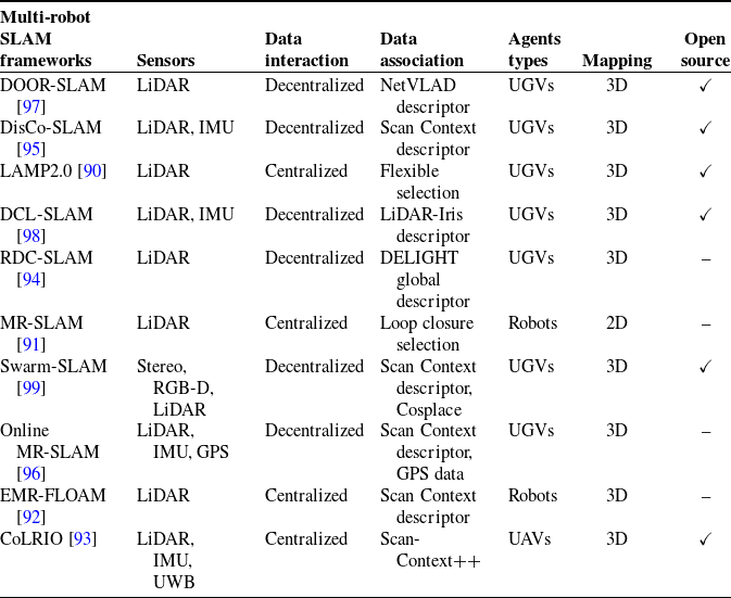
Most CSLAM systems are vision-based, such as CCM-SALM [Reference Schmuck and Chli87], C2VIR-SLAM [Reference Xie, He and Mao88], and CORB2I-SLAM [Reference Saha, Dhara and Umer89], but research on LiDAR CSLAM is relatively limited. LAMP 2.0 [Reference Chang, Ebadi and Denniston90] is a typical LiDAR-centric multi-robot system that has been experimented with in unknown large-scale underground environments. It combines a single-robot front-end interface that can adapt to different range sources and LiDAR configurations and a scalable multi-robot front-end that can support large-scale environments and multi-robot inter- and intra-loop closure detection. Liu et al. [Reference Liu, Li and Li91] proposed a centralized multi-robot collaborative LiDAR SLAM framework, in which each robot is equipped with only one 2D LiDAR and a loop closure selection method is used to ensure the correctness and consistency of global optimization. Jalil [Reference Jalil and Ibraheem92] proposed an enhanced multi-robot fast localization, ranging, and mapping algorithm (EMR-FLOAM), which uses a two-stage non-iterative distortion compensation technique to address computational complexity and resource requirements. Zhong et al. [Reference Zhong, Chen and Qi93] proposed CoLRIO, an online, centralized, and robust collaborative SLAM framework, which enables multiple robots to generate global SLAM estimates in real-time from simultaneously collected data and achieve co-localization without deploying anchors.
3.1.2. Decentralized CSLAM
In the decentralized CSLAM approach shown in Figure 9(b), the decentralized system typically consists of several interconnected robots that are managed by a coordinating architecture and can communicate with other robots to share environmental information, poses, or maps. Distributed systems can cope with partial failures, and even if some distributed robots fail or lose contact, other robots can still complete the task or at least part of the task.
A notable advantage of distributed systems is the capability to alleviate the bandwidth burden. Xie [Reference Xie, Zhang and Chen94] developed a real-time distributed collaborative SLAM system based on 3D LiDAR: RDC-SLAM, which uses the DELIGHT global descriptor instead of traditional point cloud matching, significantly reducing the communication bandwidth and time consumption pressure between multiple robots. Huang et al. [Reference Huang, Shan and Chen95] proposed a distributed multi-robot SLAM, DiSCo-SLAM, which is the first to apply scan context descriptor to multi-robot SLAM and 3D LiDAR observation, including a global-local optimization framework. The system is suitable for low communication bandwidth scenarios. Xie et al. [Reference Xie, Zhang and Hu96] proposed an online multi-robot LiDAR system that hierarchically divides the path planning problem into global planning and local navigation. However, it requires LiDAR and Global Positioning System (GPS) data for data association and is only applicable to partially unknown environments.
DOOR-SLAM [Reference Lajoie, Ramtoula and Chang97] is a fully distributed SLAM system consisting of two parts: position graph optimization and distributed SLAM front-end. It uses point-to-point communication, performs distributed outlier rejection to remove false loop closures, and performs distributed pose graph optimization to retrieve the robot’s trajectory estimate. Also based on point-to-point communication, DCL-SLAM [Reference Zhong, Qi and Chen98] focused on data-efficient and resilient communication between robots, enabling consistent trajectory estimation through partial attitude measurement and indirect data association. Swarm-SLAM [Reference Lajoie and Beltrame99] is an open-source CSLAM system specifically designed for swarm robots that emphasizes scalability, flexibility, decentralization, and sparsity, with a new budget approach to select inter-robot loop closure to reduce data exchange.
Table III summarizes several classic CSLAM frameworks. However, decentralized or distributed systems are also limited by the on-board computing and communication of robots, which brings additional challenges such as complex data management capabilities and bookkeeping strategies, information double counting, and high latency [Reference Ahlström and Schmidt100].
3.2. Key issues of CSLAM
3.2.1. Robust data association
Robust data association is the key technology to promote multi-autonomous robot collaboration. Data association refers to matching current sensor data with stored map data (or map data shared by other robots) to find the correct corresponding points or features [Reference Liu101], which is usually done at the front end of collaborative SLAM. Robust data association can effectively handle factors such as sensor noise, occlusion, and dynamic scene changes, avoid mismatching, and ensure the accuracy and stability of the multi-robot SLAM system.
Summary of the most representative multi-robot SLAM frameworks.

In multi-robot LiDAR SLAM, LiDAR sensors are used to map the environment, which usually generates a point cloud dataset. Data association involves the following aspects: (1) point cloud registration: avoiding local mismatches and large-scale drift [Reference Li, Guo, Yi and Hong102]; (2) sparsity of point clouds: sparse point cloud data has a low density and it is difficult to provide sufficient feature information for effective matching. The ICP algorithm and its various variants are known point cloud registration application methods but are only suitable for single-robot SLAM to calculate relative poses and are not well suited for multi-robot operations because they rely on a good initial guess, which is usually not available between the local maps of the robots.
The data association of the LiDAR CSLAM system is divided into feature matching and direct matching methods. Direct matching methods include: probabilistic model NDT with poor predictability [Reference He, Jia and Hong103], correlation matching method ICP with high computational complexity, etc. Feature matching methods perform data association and pose estimation based on the features with high significance in the LiDAR scan, and align the relative pose by aligning two LiDAR scans to improve computational efficiency. 3D feature description is similar to image matching, but due to problems such as disordered organization, uneven density, lack of texture, and structural occlusion, dense point cloud information often contains more redundant data, and the outliers of 3D feature matching are very high. In addition, the descriptor-based method has high computational complexity and is difficult to process in real-time.
Shin et al. [Reference Shin, Park and Kim104] argued that relatively sparse point clouds have no meaning for the depth associated with visual features. They apply the direct method to the combination of low-line LiDAR and camera to realize a loosely coupled SLAM system and solve the sparsity problem in data association. Xie et al. [Reference Xie, Zhang and Chen94] proposed a descriptor-based approach to multi-robot SLAM and designed a communication protocol to facilitate data association between robots. However, with the increase in running time, descriptor matching time increases, making it difficult to guarantee the real-time performance of SLAM.
Perceptual aliasing can lead to incorrect inter-robot data association. Tian et al. [Reference Tian, Chang, Arias, Nieto-Granda, How and Carlone105] introduced a multi-robot system called Kimera-Multi that can identify and reject incorrect inter-robot and intra-robot loops caused by perceptual aliasing, improving global mapping consistency. Liu et al. [Reference Liu, Bi, Shi, Zhang and Wang106] introduced a semantically assisted LiDAR tightly coupled SLAM method that incorporates constraints based on semantic information in the point cloud feature extraction and matching process to improve the accuracy and pose estimation precision and promote globally consistent map construction.
3.2.2. Inter-robot loop closures
The CSLAM front-end is responsible for generating landmark estimates, odometry measurements, and loop closures within and between robots. The computation of odometry and intra-robot loop closure measurements can be done completely locally on each robot [Reference Yan, Lin and Ren107]. Loop closure detection, also known as place recognition, refers to the robot group identifying the places they have visited before and performing data correction to eliminate drift errors. Incorrect loop closures can cause robots to connect their current location to a different location they visited previously, resulting in incorrect data association and global inconsistency issues. Correct loop closures can significantly reduce cumulative errors, helping robots avoid obstacles more accurately and quickly, especially in large-scale environments. Establishing closed-loop detection between robots requires a lot of key human resources to exchange sensor data.
The generation of inter-robot loops is crucial to ensure estimation consistency. Inter-robot closure detection can be divided into two forms: direct and indirect. Direct inter-robot closure detection is to calculate the relative pose based on the position coordinates when the robots meet, but this process is called “rendezvous.” After the robots meet, they exchange observation data to identify potential loop closures. Finding an optimal lossless swap strategy (i.e., a minimum weighted vertex cover) is NP-hard. Tian et al. [Reference Tian, Khosoussi and Giamou108] proposed a resource-adaptive framework for distributed loop closure detection to address the resource consumption problem in inter-robot loop closure detection, enabling rendezvousing robots to collaboratively search for loop closures between robots by exchanging a near-optimal subset of their observations without exceeding the allocated data transmission budget.
Indirect inter-robot closure detection estimates the corresponding transformation by reviewing the overlapping regions in the maps. After the location recognition matching, geometric estimation is performed to calculate the relative pose between the two locations. A common method for robots equipped with 3d LiDAR to perform location recognition is to use compact and robust global point cloud descriptor matching, such as Scan Context descriptor, global descriptor LiDAR-Iris [Reference Zhong, Qi and Chen98], etc. The similarity score between the global descriptors from the two robots is calculated to identify the locations or overlapping parts between their respective maps. Wang et al. [Reference Wang, Wang and Xie109] proposed a robust loop closure detection method and a global three-dimensional descriptor to improve robot mapping accuracy, but it was only applied to a single robot. Feature-based visual CSLAM [Reference Zhu, Xu, Wang, Liu and Tian110] uses the bag-of-words (BoWs) approach to find multi-robot loop closures. Shan et al. [Reference Shan, Englot, Duarte, Ratti and Rus111] proposed a method for robust real-time place recognition using imaging LiDAR, extracting ORB feature descriptors from images and encoding them into BoWs vectors, which can quickly and robustly search for loop closures and produce 3D point clouds with image quality and high resolution.
Chen [Reference Chen, Zhao and Feng112] proposed an inter and intra-robot loop closure selection algorithm based on robust consistency for multi-robot pose graph map fusion, which provides initial relative pose estimation between robots by introducing a new consistency score and based on a consistent loop closure selection strategy. LAMP2.0 proposed a modular loop closure method that can adapt to various environmental representations (2D grid maps and 3D maps). DCL-SLAM used the Iris descriptor derived from LiDAR data and uses the Hamming distance and KD tree method for loop closure detection. Swarm-SLAM proposed a new inter-robot loop closure priority technology that can reduce communication and accelerate convergence.
3.2.3. Global optimization
CSLAM backend optimization is an effective way to reduce the accumulated local errors in front-end matching. The backend solves nonlinear pose graph optimization, and global graph optimization generates a global factor graph to consistently and effectively represent the information of multiple robots [Reference Ebadi, Bernreiter and Biggie113]. The pose graph uses the robot pose (position and orientation) as the nodes in the graph, and the robot motion constraints (odometer data) and loop detection constraints as the edges in the graph.
Pose graph optimization (PGO) is an effective method for global optimization. PGO methods [Reference Shin, Sim, Nam, Kim, Heo and Kim114, Reference Bai, Yuan, Guo, Yin, Yau and Xie115] are also divided into centralized and distributed types. Centralized PGO collects all measurements at a central station, which is responsible for calculating the trajectory estimates of all robots. However, when the number of robots increases, problems such as excessive computational burden on the central station, reduced optimization speed, and high communication overhead will be encountered. Distributed PGO is more suitable for multi-robot systems. Each robot only maintains the pose and edges related to itself and performs local optimization. Finally, a distributed optimization algorithm is used for collaborative calculation to converge to a consistent global optimal solution.
Choudhary et al. [Reference Choudhary, Carlone, Nieto, Rogers, Christensen and Dellaert116, Reference Choudhary, Carlone and Nieto117] proposed a distributed two-stage Gauss-Seidel method, which iteratively recovers the posture by decoupling the rotation and translation components. However, this method has high initialization requirements and cannot guarantee convergence to the first-order critical point. Fan and Murphey [Reference Fan and Murphey118] proposed an optimization minimization method for distributed PGO that is guaranteed to converge to the first-order critical point under mild conditions. Li et al. [Reference Li, Guo, Yi and Hong102] proposed a distributed pose graph optimization algorithm that combines multi-level partitioning and accelerated optimization methods. The communication overhead of multi-robot parallel computing is reduced by balancing the posture graph. Based on the non-convexity of the PGO problem, the IRBCD method is used to quickly converge to the optimal solution. Optimizing the global coordinate transformation graph can ensure high-quality initial guesses, thereby stably and accurately optimizing the local pose graph of the robot. Disco-SLAM [Reference Huang, Shan and Chen95] contains a two-stage global-local optimizer. In the global optimization, the factor graph containing the transformation of the robot’s local frame to the global frame is optimized. In the local optimization, the local pose graph of the robot’s local odometry, the robot’s internal constraints, and the constraints between adjacent robots are optimized.
4. Challenges of MRS sub-fields
At present, CSLAM is based on multi-robot systems execution of mapping tasks. For multiple robots that make up a robot cluster, the pose and position of each robot are first estimated and calculated, that is, localization. The frontier exploration strategy is used for frontier detection, and tasks are assigned to each robot through the task allocation algorithm. The robots go to the target points for exploration according to the assigned task and use the environmental data information sensed by their sensors to build their local map, which is then fused to obtain a global map.
The framework diagram of multi-robot SLAM is depicted in Figure 10. After each function, the content and details of the global map will increase until the exploration ends. Compared with single-robot SLAM, multi-robot SLAM expands three key sub-fields: frontier detection, task allocation, and map fusion.
Multi-robot SLAM workflow framework. The framework includes three core issues: frontier detection, task allocation, and map fusion. The robot teams perform exploration tasks in a global coordinate system.

4.1. Frontier detection
Frontier detection is a widely used exploration method that plays a crucial role in identifying frontiers, which act as boundaries between explored and unexplored regions on the global map. As illustrated in Figure 11, the frontier refers to the boundary between the unknown area and the known area in the current map, which consists of a set of unknown points. In frontier-based exploration, each point is connected to at least one open space. The robot engages in exploration by continuously detecting and navigating toward these boundaries, which separate familiar regions from unexplored areas. Frontier detection involves the identification of boundaries between unknown areas and known areas without obstacles on the map. The significance of frontiers lies in determining optimal locations for the robot’s future exploration within the environment [Reference Oršulić, Miklić and Kovačić119].
Frontier-based exploration process. The unknown area refers to the gray area around the map, and the known area is the obstacle (such as a wall) detected by the black line on the left. The frontier is the boundary between the known and unknown areas marked in red, the open space is the area to be explored on the right, and the occupied space is the gray portion marked by the black border in the middle of the map (such as obstacles).

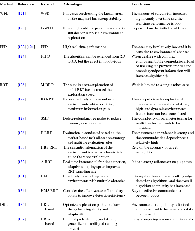
Yamauchi [Reference Yamauchi120] introduced the concept of boundaries and pioneered active exploration based on boundary detection and tracking. Yamauchi’s work involved each robot moving towards the centroid of the nearest boundary. The robots independently navigate toward the target while sharing a common map, and boundary detection is performed only upon reaching the target. This work laid the foundation for future mobile robots to explore unknown maps. Subsequently, detected boundaries have become commonly used as navigation targets for mobile robots in exploration mission planning. Building on this foundation, more sophisticated exploration strategies have emerged. Table IV provides a summary comparing different boundary detection algorithms.
Algorithms of frontier detection.

4.1.1. WFD, FFD
Early scholars used image processing technology, such as Canny edge detection, to extract boundary points from map images. Once the boundary is detected, the frontier on the boundary will be assigned as targets for the robot to explore. However, this method is only suitable for small-scale scenes. When the scene gets large, the efficiency of the image processing process for the entire scene will be significantly reduced.
Most early frontier detection algorithms dealt with the entire map data. This process was time-consuming and could impact exploration decisions. Keidar and Kaminka proposed the Wavefront Frontier Detector (WFD) and the Fast Frontier Detector (FFD) [Reference Keidar and Kaminka121, Reference Keidar and Kaminka122] to address this issue. The WFD algorithm is a graph-search-based approach that focuses on examining known areas of the map. Limiting the analysis to known areas reduces the computational burden compared to processing the entire map. The WFD algorithm efficiently detects frontiers by examining the boundaries between known and unknown regions. However, as exploration progresses, the known area that needs to be processed becomes larger. The FFD algorithm only extracts the exploration frontier each time it acquires sensor data. However, it can only extract new frontiers from sensor data when the robot obtains unknown environmental information.
Quin [Reference Quin, Alempijevic, Paul and Liu123] extended the WFD algorithm by utilizing the frontier cells from the previous time step as the starting point for detecting the frontier in the current time step. This extension combines the ideas of WFD and FFD. Instead of exploring all unoccupied areas like FFD, it searches for new unoccupied regions. In addition, the Frontier-Tracing Frontier Detection (FTFD) algorithm proposed by Quin et al. [Reference Quin, Nguyen and Vu124] uses the perimeter observed by the current sensor combined with the laser scanning endpoint and the previously known boundary to perform boundary detection. FTFD is suitable for applications that require frontier detection after each observation and can be extended from 2D to 3D, but the effect is not obvious. Sun et al. [Reference Sun, Wu, Xu, Sarma, Yang and Kong125] extended the DFD method [Reference Oršulić, Miklić and Kovačić119] by first expanding the submap and using WFD to detect the local reachable frontier, and adaptively selecting the span according to the posture deviation of the submap, which is more effective and flexible than the DFD method.
4.1.2. RRT
The Rapid Random Tree (RRT) algorithm is currently one of the most mainstream boundary-based exploration methods for robot autonomous exploration. Umari [Reference Umari and Mukhopadhyay126] proposed using RRT for boundary detection. RRT involves random sampling within a specified region and creating tree edges and nodes based on the sampled points and their nearest valid tree nodes. Through iterative iterations, a comprehensive tree-like structure is formed. This approach integrates the generation of local and global trees to effectively and efficiently select boundary points. In this method, the RRT algorithm is utilized for boundary point selection, performing path planning on a global scale and refining it locally.
Pimentel [Reference Pimentel, Alvim, Campos and Macharet127] enhanced the traditional RRT algorithm by incorporating Shannon entropy to estimate the expected information gain (ID-RRT) for each candidate boundary. Their approach generates paths for navigation to selected destinations. Zhang [Reference Zhang, Lin, Wang and He128] extended the RRT algorithm by introducing a cost function that considers passing through unknown and unexplored regions. The trajectory length from the initial position to the target frontier point is defined as an unconstrained optimization problem.
However, the randomness of the RRT algorithm may cause some boundary points to fail to be detected in time, resulting in backtracking. Therefore, Qiao [Reference Qiao, Fang and Si129, Reference Qiao, Fang and Si130] introduced a multi-tree fusion algorithm called Sample-based Multi-tree Fusion (SMF), which combines sampling with RRT. SMF retains tree nodes while discarding tree edges after boundary detection, allowing the tree to grow across obstacles. The proposed block structure significantly reduces the number of tree nodes stored in the search process, thus reducing the memory consumption. Xu et al. [Reference Xu, Zhang and Chen131] proposed an autonomous exploration strategy based on hybrid frontier detection to deal with large-scale environment problems with multiple obstacles. It consists of a variable step-size random tree global frontier detector, a multi-rooted random tree boundary detector, and a grid-based boundary detector. With the increase of expansion, the number of nodes is increasing, which affects the exploration efficiency. Sun et al. [Reference Sun, Wu and Xu132] proposed an efficient frontier detector method based on adaptive RRT to achieve real-time incremental frontier detection. Its adaptive sampling space improves the successful sampling rate of RRT. The detector tends to sample in the newly explored area, which improves the efficiency of boundary detection.
The discrete detection strategy based on the RRT algorithm ignores the geometric continuity of the environment, resulting in disordered robot motion, and the efficiency of the traditional RRT algorithm decreases as the exploration area increases. To address this problem, Liu [Reference Liu, Lv, Yuan, Chi, Chen and Sun133] proposed a heuristic-based biased sampling robot exploration strategy, which uses the connection between environmental semantic information and geometric heuristics as heuristic information to guide robot exploration. After obtaining the estimated area of the heuristic object, a biased RRT algorithm is proposed to accelerate the frontier detection of the estimated area.
Furthermore, Ning [Reference Ning, Li, Yao, Du and Zhang134] proposed a frontier detection algorithm based on a hybrid multi-strategy RRT. This method combines an adaptive distance increment strategy, subregion sampling strategy, and greedy boundary exploration strategy. The effectiveness of the identified boundary points is carefully considered, resulting in enhanced detection efficiency.
4.1.3. DRL
Currently, deep reinforcement learning (DRL) is in a boom state. The traditional heuristic method is efficient and easy to use, but it is limited to specific cases. Because they lack the ability to integrate the intentions of teammates, they perform poorly in decentralized execution. Due to the use of manually designed utility functions and the lack of structural information in the field, these methods are difficult to be extended to different chaotic fields. Therefore, the advantages of deep reinforcement learning are embodied [Reference Mete, Mouhoub and Farid135]. Leong [Reference Leong136]’s method optimizes the robot’s movement through reinforcement learning and uses a reward mechanism to guide the robot to select the optimal frontier point. Compared with traditional frontier exploration strategies, it can effectively improve the problem of non-optimal paths in scenarios with multiple frontiers and similar distances, enabling the robot to choose a more reasonable path during the exploration process and improve exploration efficiency. Wang [Reference Wang, Zhang and Lyu137]’s enhanced frontier exploration method, combined with DRL, uses global and local networks to extract map features, allowing the robot to better understand the environment than traditional boundary-based methods and complete exploration at a lower distance cost.
4.2. Task allocation
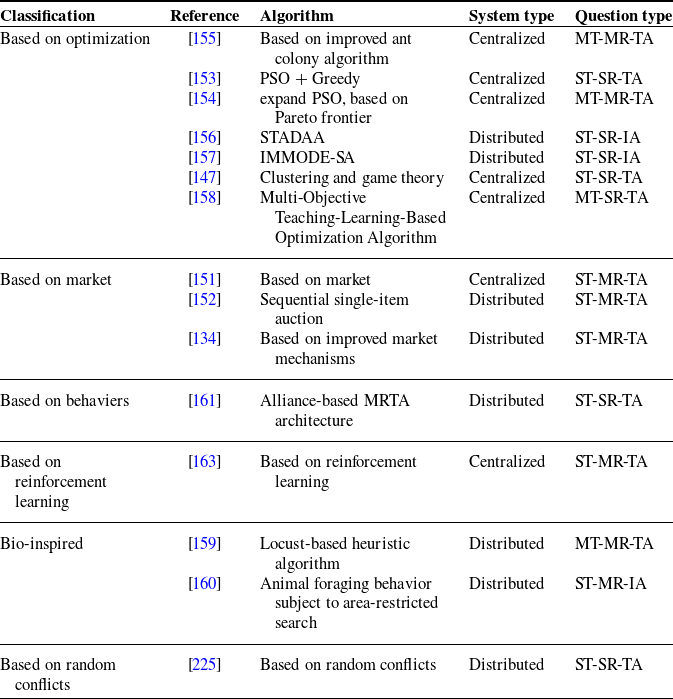
Through frontier detection, several target points need to be explored by robots, and these target points need to be reasonably allocated to multiple robots to complete the SLAM task under the condition of optimal target. How to assign appropriate tasks to different robots to optimize the objective function is a process called Multi-Robot Task Allocation (MRTA) [Reference Khamis, Hussein and Elmogy138]. MRTA is characterized as a combinatorial optimization problem that aims to identify the optimal solution from a finite set of feasible solutions. The objective function in MRTA operates on a discrete domain with a vast search space.
Each robot explores based on simple criteria for the nearest boundary, which can lead to problems with repeated exploration and even collisions. Therefore, we need to allocate the boundary points reasonably through evaluation. A single factor is not sufficient to effectively disperse multiple robots between tasks, and the expected costs and benefits of executing each candidate boundary point must be estimated. Evaluating all boundary points to estimate the effect of performing a set of actions to reach each boundary point is utility computing [Reference Scheler and Dietrich139]. The commonly used methods of utility evaluation include information theory (IT), optimal experimental design theory (TOED), etc. Gao [Reference Gao, Booker, Adiwahono, Yuan, Wang and Yun140] designed a new utility function that considers the optimal frontier allocation of the robot’s moving distance, boundary size, and turning cost. By constructing a topological graph and recording the key nodes visited and unknown states, this method can better balance map coverage and time consumption. Sun et al. [Reference Sun and Zhang141] proposed a detection and maintenance method for incremental addition of frontiers and a multi-path generation method, using the proposed multi-objective utility function for frontier evaluation to obtain the optimal path and improve exploration efficiency.
In addition, after the task assignment, the robot also needs to perform corresponding path planning. RRT algorithm and A* algorithm are both commonly used path planning algorithms. Fusic [Reference Fusic and Sitharthan142] introduced an improved fast random tree (IRRT*) algorithm, which uses triangle inequality rewiring technology to find collision-free paths for drones in three-dimensional environments. After that, they [Reference Fusic and Sitharthan143] proposed a mobile robot path planning method based on adaptive learning particle swarm optimization, aiming to find the most effective path in an obstacle environment mapped by LiDAR. For a more detailed review of path planning, please refer to [Reference Hichri, Gallala and Giovannini144, Reference Reda, Onsy and Haikal145]. This section focuses on the relevant algorithms for task allocation.
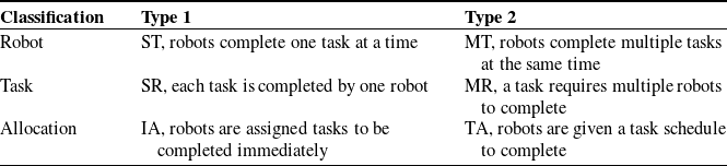
Multi-robot task allocation can be classified into single-task (ST) and multi-task (MT) based on the number of tasks a robot can handle concurrently. Additionally, they can be categorized as single-robot task or multi-robot task (MR), depending on the number of robots required for each task. In terms of the time plan, assignments can be further divided into instantaneous assignments and time-extended assignments (TA) [Reference Sarkar, Paul and Pal146, Reference Martin, Muros, Maestre and Camacho147]. The classification criteria are summarized in Table V.
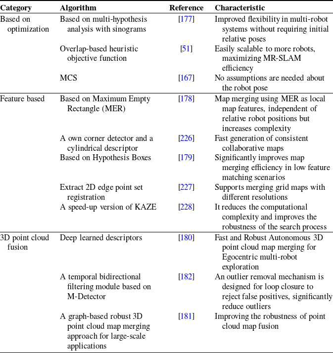
Multi-robot task allocation categorization.

Scholars at home and abroad have conducted in-depth research on the multi-robot task allocation problem and proposed various algorithms and variants. The currently popular task allocation algorithms can be roughly divided into five categories: market-based allocation strategies [Reference Quinton, Grand and Lesire148], optimization-based [Reference Chakraa, Guérin, Leclercq and Lefebvre149], bio-inspired, behavior-based [Reference Seenu, K.C., Ramya and Janardhanan150] allocation strategies, and reinforcement learning-based allocation strategies. We review some classic task allocation algorithms and compare them in Table VI.
Algorithms of task allocation.

4.2.1. Market-based
Market-based strategies, inspired by economic theory, provide an effective approach for coordinating robot activities and are commonly used to solve MRTA problems. Auctions, which consider robot bids and auction criteria (objective functions), are employed to allocate tasks to robots. Market-based methods utilize robust communication mechanisms for coordination, with a central unit collecting auction bids and performing task assignments [Reference Quinton, Grand and Lesire148]. In these strategies, robots are treated as bidders and tasks as commodities. Robots detect boundaries and bid on them, adding the won boundaries to the task list of the winners. Tasks for each robot are sorted based on their new auction prices at each iteration [Reference Yu, Deng, Yao, Zhu and Gui151]. Please refer to the works of De Ryck [Reference De Ryck, Pissoort, Holvoet and Demeester152], Yu [Reference Yu, Deng, Yao, Zhu and Gui151], Ning [Reference Ning, Li, Yao, Du and Zhang134], and others for more details on market-based strategies for multi-robot task allocation.
4.2.2. Optimization-based
The optimization-based task allocation strategy generalizes the dynamic MRTA problems into multiple traveling salesman problems and classifies them as combinatorial optimization problems. Multi-objective optimization tasks improve the task completion rate in less time but have poor adaptability to objective factors and low robustness. Classic optimization-based strategies include the ant colony algorithm, particle swarm algorithm [Reference Kong, Gao, Wang, Liu and Xu153, Reference Wei, Ji and Cai154], and their variants.
The basic ant colony algorithm suffers from slow convergence and a tendency to get stuck in local optima. Qin [Reference Qin, Zong, Li, Zhang and Zhang155] addressed these issues by introducing a local optimization mutation operator and an improved simulated annealing algorithm. The mutation operator was used for local optimization, and the algorithm employed the Metropolis criterion from the simulated annealing mechanism to probabilistically accept worse solutions. This allowed the algorithm to escape local extreme values and achieve better optimization results, while also exhibiting faster convergence speed.
Lindsay [Reference Lindsay, Buehling and Sun156] proposed a Sequential Task Addition Distributed Allocation Algorithm that enables fast and scalable allocation in a specific class of MRTA problems. However, its applicability is limited to this particular class of problems. Miao [Reference Miao, Huang, Jiang and Fan157] proposed an improved multimodal multi-objective differential evolution algorithm hybrid with a simulated annealing algorithm to solve MRTA problems. Martin [Reference Martin, Muros, Maestre and Camacho147] introduced a cooperative game framework to address MRTA problems. They established a cooperative game to evaluate the performance of robots and task sets. In their experiments, they compared the performance and computation time of their game theory-based approach against a benchmark genetic algorithm. The results showed that the game theory-based method outperformed the genetic algorithm in terms of performance and computation time. Kang [Reference Kang, Miao and Pan158] proposed a teaching-based multi-objective optimization algorithm and established a mathematical model to study the task allocation problem of multiple weeding robots.
4.2.3. Bio-inspired
Bio-inspired algorithm is a method to solve the task assignment problem by drawing on the self-organization, adaptability, and optimization ability of biological system. Bionic algorithms are typically rooted in the concept of swarm intelligence, which involves abstracting a problem into the interactions and cooperation among individuals. These algorithms aim to find optimal solutions by simulating the behaviors exhibited by biological groups. Kurdi [Reference Kurdi, Aloboud, Alalwan, Alhassan, Alotaibi, Bautista and How159] proposed a novel autonomous bionic method for allocating tasks among multiple drones during a mission. Aljalaud [Reference Aljalaud and Kurdi160] proposed a multi-UAV task allocation system inspired by area-restricted search, which is inspired by animal foraging behavior, that is, after finding prey, animals usually spend more time searching in the nearby area to maximize food intake. The algorithm shows better net throughput than the baseline performance, especially in the case of small fleet size, without affecting runtime performance.
4.2.4. Behavior-based
Behavior-based dynamic task allocation assumes that the frontier is attractive to robots, while obstacles and other robots are repellent. The multi-robot exploration problem involves a two-layer behavior-based control structure, where task identification and inter-robot communication are referred to as high-level behaviors, and obstacle avoidance, navigation, and task switching are referred to as low-level behaviors. When necessary, high-level behaviors can inhibit or prevent low-level behaviors. This strategy is particularly well-suited for MRTA in scenarios with weak communication capabilities and uncertain, dynamic real-world environments. Dos [Reference dos Reis, Lopes and Bastos161] proposed an axiomatic framework based on Social Choice Theory to analyze the task allocation problem in intentional cooperation multi-robot systems.
4.2.5. Reinforcement learning-based
The reinforcement learning-based approach [Reference Alitappeh and Jeddisaravi162] makes decisions by learning from the behavior of other robots, but it may suffer from overfitting to specific environments. Commonly used reinforcement learning techniques include Q-learning. Task allocation strategies based on reinforcement learning present a promising direction for further research. By employing a reward strategy, rewards or penalties are assigned based on the chosen actions. Park [Reference Park, Kang and Choi163] proposed a Markov decision process model for multi-robot task allocation using reinforcement learning to address the problem that the performance of existing metaheuristic methods deteriorates as the number of robots or tasks increases. The proposed formula follows a sequential assignment approach, aiming to minimize the overall completion time of the tasks. It incorporates a cross-attention mechanism to determine the preference of robots for each task. This enables the algorithm to identify the optimal allocation solution for each problem and improve the solution quality, especially when dealing with large-scale allocation problems.
DRL combines the powerful nonlinear function-fitting capabilities of deep neural networks with the decision-making and control abilities of reinforcement learning, offering a novel approach to solving the multi-agent task planning problem. Xie et al. [Reference Xie, Yang and Xiao164] used DRL to solve the three-dimensional path planning problem of UAVs. Zhang et al. [Reference Zhang, Ren and Cui165] proposed a multi-unmanned surface vessel (USV) mission planning method based on improved DRL to solve the problem of how to design a suitable reward function in mission planning. Jin et al. [Reference Jin, Sun and Wu166] proposed a multi-robot collaborative path planning and task allocation method based on a dual deep Q-learning network and ant colony optimization algorithm in a 3D environment.
4.3. Map fusion
Map fusion can be viewed as a specialized instance of image registration in computer vision, wherein the image corresponds to a map with a distinct geometric structure. Occupancy grid maps, which consist of matrices storing the probability of each grid cell being occupied, are commonly used in this context [Reference Sun, Sun, Yu and Peng167]. By treating each value in the occupancy grid map matrix as a pixel in an image, the representation of grid map fusion becomes analogous to image fusion. Grid map fusion is a crucial challenge in both multi-robot SLAM and single-robot SLAM. In computer vision, the process of merging occupancy grid maps is transformed into an image registration problem by establishing an objective function to calculate the transformation matrix.
Occupancy grid maps have been the subject of extensive research, and various merging methods have been proposed. These methods include probabilistic methods, optimization-based techniques, and feature-based methods. In addition, map merging algorithms have gradually evolved from 2D to 3D point clouds. This paper focuses on feature-based map fusion methods.
The feature-based method consists of three stages: feature detection, feature description, and feature matching. Common feature detection methods include SIFT detector [Reference Lowe168], SURF detector [Reference Bay, Ess, Tuytelaars and Van Gool169], ORB detector [Reference Rublee, Rabaud, Konolige and Bradski170], Accelerated-KAZE (AKAZE) detector [Reference Qu, Bu and Liu171], etc. Common feature description methods include SIFT, SURF, Brisk [Reference Leutenegger, Chli and Siegwart172], Freak [Reference Alahi, Ortiz and Vandergheynst173], etc. In the feature matching stage, the Random Sample Consensus [Reference Chum and Matas174] method is often used for fine matching, and the transformation matrix T is calculated based on the matched feature pairs to perform image transformation and fusion.
Early methods for multi-robot map fusion represented advancements over existing single-robot map fusion techniques adapted for multi-robot systems. Thrun [Reference Thrun175] used a combination of maximum likelihood estimation and particle filters to create a consistent global grid map on multiple robots, but this required the relative initial positions of multiple robots to be known and had high requirements for data communication. Subsequently, Howard [Reference Howard176] used Rao-Blackwellized particle filters for grid map fusion and did not require the initial positions of the robots to be known. Table VII presents a comprehensive summary and comparison of various map fusion algorithms.
Algorithms of map fusion.

4.3.1. Optimization-based methods
Optimization-based methods aim to find the best map configuration through optimization algorithms (such as particle swarm optimization, genetic algorithms, etc.) or objective functions. Lee [Reference Lee, Roh and Lee177] proposed a sinogram-based particle swarm optimization multi-hypothesis map merging algorithm to address the challenge of merging maps without features, local maxima, and initial relative pose information. Wang [Reference Wang, Shang and Gao51] proposed a heuristic search method to guide the fusion of repeated areas of local maps. Each robot sends local map information to the same workstation, and uses the similarity of local maps as the judgment indicator for fusion to obtain the optimal global map.
4.3.2. Feature-based methods
Feature-based methods are one of the most commonly used map fusion methods. The feature-based map fusion method is as follows: After obtaining the local maps of the two robots, the images can be preprocessed, such as binarization, to make the detected feature points more accurate. Next, the feature points of the two maps are detected and described, and then the feature points are matched. According to the matched feature point pairs, the transformation matrix T is calculated. After obtaining T, the image is translated or rotated according to T, and finally, the map is fused to obtain the global map. Figure 12 shows a process flow chart of feature-based map fusion.
Common features include points, lines, surfaces, and some geometric features such as triangles and rectangles. Sun [Reference Sun, Sun, Yu and Peng167] proposed a map fusion algorithm based on the maximum common subgraph (MCS), which uses Harris corner points to extract corner points from the grid map, constructs a triangular isomorphic graph, calculates the initial optimal transformation matrix, and finally iteratively finds the MCS in the generated polygonal isomorphic graph and optimizes the transformation matrix. Jazi [Reference Jazi178] proposed a map merging algorithm based on the maximum empty rectangle (MER). Map merging is performed by constructing the MER as a local map feature. Experimental results show that the algorithm can merge local maps with a small overlapping area relative to the entire map. However, the sensitivity of the MER to rotated maps increases the complexity of the fusion process. Chen [Reference Chen, Li, Zhao and Liu179] proposed a hypothesis-based map fusion method. First, they extracted rectangular corners based on their shared edge features and constructed virtual bounding boxes in the map. Then, they obtained a transformation matrix based on a matched pair of virtual bounding boxes and optimized the transformation matrix using a KF. Wang [Reference Wang44] applied AKAZE to map fusion, using the AKAZE features of overlapping areas to estimate the relative pose of the robot, described by the modified local difference binary descriptor. The algorithm reduces the computational complexity and improves the robustness of the search process.
Flow chart of feature-based map fusion.

4.3.3. 3D point cloud fusion methods
3D maps are now crucial in various applications of mobile robots, and SLAM can generate dense 3D point cloud maps (PCM). Stathoulopoulos [Reference Stathoulopoulos, Koval, Agha-mohammadi and Nikolakopoulos180] proposed a 3D point cloud map merging framework based on overlap detection and alignment for egocentric heterogeneous multi-robot exploration that does not rely on manual initial guesses or prior knowledge of the robot poses. Their solution leverages unknown recognition learning descriptors to provide fast and robust region overlap estimation through the framework’s main pipeline, eliminating the need for time-consuming global feature extraction and feature matching typically used in 3D map integration. Gui [Reference Gui, Zeng and Luo181] introduces a graph-based robust 3D PCM merging method for large-scale applications. Wei et al. [Reference Wei, Li, Cai, Yuan, Ren, Zou, Wu, Zheng, Zhou, Xue and Zhang182] propose an emerging 3D point cloud map merging framework, design a temporal bidirectional filtering method to remove dynamic objects from 3D LiDAR point cloud data, and use a binary triangle combination descriptor to provide accurate location description, thereby improving the accuracy of the merged result.
5. Open questions of LiDAR SLAM
With the further development of multi-robot LiDAR SLAM technology, based on the existing technology, its future development trends include the following aspects.
5.1. Challenges and solutions in unstructured scenarios
Robots have achieved relatively high levels of autonomy in controlled and static environments. However, in unstructured environments, complex environmental perception makes it challenging to develop fully autonomous mobile robots. Liyana et al. focused on the problems of robot perception and scene understanding in unstructured environments and their applications in related positioning, mapping, and path planning, and conducted an extensive literature review [Reference Wijayathunga, Rassau and Chai183]. Min et al. [Reference Min, Si and Wang184] discussed autonomous driving technology in unstructured environments, including challenges such as environment perception, pose estimation, and mapping, and pointed out the future research direction of autonomous driving technology in unstructured scenarios.
Robot perception, scene analysis, and deeper scene understanding are key issues for autonomous robot navigation in unstructured outdoor environments. In some unstructured environments and dynamic scenes with uneven terrain and cluttered objects, there are many limitations on robot perception capabilities. Vision-based SLAM is very unstable, and feature-based SLAM will also cause feature loss due to some dynamically moving scenes [Reference Liu, Wen, Liu and Yu185]. Under changing lighting conditions and shadows, LiDAR SLAM using point-cloud registration methods is more stable than visual SLAM and feature SLAM, but at the cost of losing some environmental semantic details. It is difficult to achieve global perception using only low-dimensional LiDAR feedback, especially in environments with highly repetitive features or rich semantic information. Therefore, heterogeneous multi-robots equipped with multiple sensors can build maps more effectively in complex environments [Reference Bayer, Cížek and Faigl186].
The combination of LiDAR SLAM and visual SLAM has been studied and applied, using visual sensors to introduce rich information and the robustness of LiDAR, and is widely used in 3D maps. Park et al. [Reference Park, Kim and Sohn187] introduced a two-stage cascade deep neural network that integrates 3D LiDAR and stereo disparity maps to yield high-precision disparities. Chen et al. [Reference Chen, Chen and Zhu188] introduced a location system based on sensor fusion, which integrated LiDAR and visual sensors, constructed a hybrid grid map for global localization, used a visual global descriptor to accelerate positioning convergence, and combined with a posture refinement pipeline to improve positioning accuracy.
RGB cameras capture high-resolution images, but lack the precision needed for accurate 3D positioning and camera motion tracking. High-resolution LiDAR systems offer precise depth estimation; however, their high cost restricts their use in various applications. Although 2D single-beam radars are more affordable, their depth estimation is insufficient for effective environmental perception. Therefore, the combination of 2D LiDAR and RGB sensors is a good feasible solution. Lu et al. [Reference Lu189] used a new self-supervised network and an economical single-beam LiDAR and camera sensor fusion to achieve performance comparable to expensive LiDAR systems. Best et al. [Reference Best, Garg and Keller190] proposed a collaborative autonomy pipeline for multi-sensor detection in constrained environments that effectively exploits range and visual sensing modalities and is resilient to adverse events.
In addition, it is crucial to build robust datasets that encompass the diversity and complexity of unstructured environments. Future work should focus on creating synthetic and real-world datasets, including dynamic and richly varied terrains, for training machine learning models. We summarize some datasets [Reference Yin191–Reference Yao, Ge and Shi195] for multi-robot autonomous navigation in unstructured scenarios to support interested researchers.
5.2. Semantic maps and deep learning in dynamic environments
Most SLAM methods assume successful execution in a static environment. Once in a highly dynamic environment, this assumption exposes the weakness of the SLAM algorithm, which lacks a module that pays special attention to dynamic objects [Reference Kenye and Kala196]. In highly dynamic environments, where large areas may be significantly occluded by objects [Reference Long, Rauch and Zhang197, Reference Long, Rauch and Ivan198], the entanglement of dynamic object features can introduce errors that can be interpolated over and over, ultimately causing the algorithm to fail. Furthermore, without loop closure, the inclusion of dynamic object features can lead to errors.
Rapid advances in deep learning in recent years have introduced novel perspectives for semantic maps-based SLAM. Integrating deep learning algorithms with visual semantic SLAM empowers robots to conduct more precise semantic segmentation, autonomously comprehend image features, identify targets, and simultaneously assess image similarity to accomplish closed-loop detection. This capability enables efficient completion of SLAM tasks in dynamic environments [Reference Wang, Tian and Chen199]. Wu et al. [Reference Wu, Guo and Gao200] proposed a dynamic environment robust visual SLAM system YOLO-SLAM, which closely combines the target detection method and the geometric constraint method to effectively reduce the impact of dynamic targets. Li et al. [Reference Li, Shen and Fu201] integrated YOLOv8’s real-time object detection and image segmentation technology into the ORB-SLAM3 framework, achieving high-precision and robust visual SLAM in dynamic environments. To address problems such as semantic inconsistency in highly dynamic scenes, Kong et al. [Reference Kong, Li and Xu202] proposed a place recognition method based on LiDAR semantic consistency, combining a LiDAR semantic image restoration network and a PR network based on a semantic pyramid transformer to perform LiDAR semantic restoration.
Currently, the method used to solve the SLAM problem in dynamic environments is mainly visual SLAM, such as RGB-SLAM. RGB-D SLAM is a more popular type of visual SLAM, especially in indoor environments [Reference Wang, Zheng and Lin203]. In addition, combined with deep learning-based semantic information, dynamic object class semantics are classified, invalid points are eliminated based on multiple loop detections, features are tracked, and local mappings are continuously corrected. Semantic segmentation is used to extract semantic information, predict labels, and generate masks for detected objects. The performance of visual SLAM in dynamic scenes can be greatly improved by identifying and removing potential dynamic objects. Blitz-SLAM [Reference Fan, Zhang and Tang204], a semantic SLAM system in dynamic indoor environments, combines the advantages of semantic and geometric information of mask, RGB, and depth images to remove noise blocks formed by moving objects in local point clouds.
Deep learning-based semantic information can solve this problem, but this method has a high computational cost and cannot handle unknown objects. Ji et al. [Reference Ji, Wang and Xie205] proposed a real-time semantic RGB-D SLAM system for dynamic environments that can detect known and unknown moving objects. The system only performs semantic segmentation on keyframes, reduces computational costs, removes known dynamic objects, and maintains stable static mapping. The learning-based semantic information method is used to handle potential dynamic objects, and an effective geometric module is proposed to handle unknown moving objects. Kenye et al. [Reference Kenye and Kala196] proposed a semantic module that can be incorporated into SLAM to identify dynamic objects, classifying semantics according to the probability that they belong to the dynamic object class. They also proposed a depth masking method based on depth-first search, which uses the depth image and the detected bounding box to generate a lower-resolution binary mask image. However, the current research in this direction is still insufficient, and there are still many points worthy of attention and exploration, such as the practical application in multi-robot systems.
5.3. Active exploration and active SLAM
SLAM research has been ongoing for decades, resulting in a relatively mature technology. However, the field of active SLAM is still in the developmental stage. Unlike traditional SLAM, active SLAM involves a decision-making process where the robot autonomously selects its future path to control its actions [Reference Placed, Strader, Carrillo, Atanasov, Indelman, Carlone and Castellanos206]. Zhang et al. [Reference Zhang, Chen and Xu207] applied the active SLAM system to improve exploration efficiency, using LiDAR SLAM and Cartographer as benchmarks for environment modeling to provide theoretical support for active exploration. Alcalde et al. [Reference Alcalde, Ferreira and González208] used deep reinforcement learning to implement active SLAM in complex environments. Taking into account map information and robot posture uncertainty, they designed a reward function based on map completeness, uncertainty, and closed loop, which improved the robot’s path planning and generalization capabilities, and provided new ideas and methods for the development of active SLAM technology.
Promising research directions include leveraging advancements in neural networks to extend the scope of SLAM beyond line-of-sight and exploring new environmental representations, as well as environmental perception and exploration-utilization balance during active exploration [Reference Singh, Kapoor and Thakur209]. Furthermore, achieving repeatability in active SLAM poses a fascinating challenge. Currently, practical applications of active SLAM are limited, and the field is in its nascent phase. However, these circumstances offer ample opportunities for future trends and advances.
5.4. Limitations of LiDAR SLAM in practical applications
While SLAM has improved its ability to adapt to the surrounding environment, traditional 2D exploration strategies remain a significant limitation, mainly for ground robots. This also limits the ability of SLAM systems to reconstruct 3D environments in the real world autonomously. In addition, the high cost of advanced SLAM systems poses a significant barrier to research and development in this field, while many low-cost SLAM systems operating in resource-constrained situations cannot achieve high-precision real-time mapping and localization, making them unsuitable for practical applications. Pang et al. [Reference Pang, Zhou and Huang210] introduce a cost-effective SLAM system design that significantly reduces costs while maintaining high performance. First, a LiDAR-inertial odometry framework is used with a fast ICP algorithm to adjust the SLAM algorithm to balance accuracy and real-time performance. The 3D multi-target RRT algorithm is combined with a nonlinear model predictive control for autonomous exploration in complex environments. Its accuracy and efficiency are comparable to those of more expensive SLAM systems, and the research results are open.
The high cost and fragility of multi-line mechanical LiDARs limit their application in real-world mapping environments. To reduce costs, multiple LiDAR odometries can be used to solve a 360-degree field of view, thereby building dense 3D maps. Chen et al. [Reference Chen, Li, Xue and Pu211] proposed a real-time, computationally efficient multi-lidar-inertial odometry system that supports multiple LiDAR settings and adopts a novel parallel state update strategy and voxelized map format to optimize computational efficiency and achieve efficient mapping.
Swarm navigation tasks [Reference Yin212] have become one of the hot research topics in the field of MRS and have been widely studied in practical applications of multi-robots. EGO-Swarm [Reference Zhou, Zhu, Zhou, Xu and Gao213] is a decentralized quadrotor swarm system that proposes a robust topology planning method to utilize onboard resources for swarm navigation. The framework is insensitive to unreliable communications and positioning drift. Park [Reference Park, Kim, Kim, Oh and Kim214] proposed an online distributed trajectory planning algorithm for a swarm of quadrotors to ensure the return of collision-free, dynamically feasible trajectories in complex environments. He conducted comparative experiments with Ego-Swarm in two obstacle environments, and the success rate was higher than that of Ego-Swarm. Swarm-LIO [Reference Zhu, Ren, Kong, Wu, Liang, Chen, Xu and Zhang215] is a fully decentralized state estimation method for aerial swarm systems. Each robot exchanges self-state estimates and mutual observation information, using 3D LiDAR for drone detection, identification, and tracking. It is applicable to various extreme environments, for example GPS-denied scenes, degenerate scenes for camera or LiDAR. The method combines LiDAR, IMUs, and mutual observation measurements to provide accurate ego state and relative state estimation. Swarm-LIO2 [Reference Zhu, Ren, Yin, Kong, Liu, Xue, Liu, Cai, Lu, Li and Zhang216] is an extension of this work, further improving the scalability of the group and showing excellent robustness in LiDAR degradation scenarios.
The SubT Challenge seeks to develop novel integrated solutions capable of mapping and navigating complex and dynamic terrain, sensors, and computation for perception in adverse conditions, distributed information sharing in degraded communications environments, and collaborative autonomy for extended operations with minimal human intervention [Reference Chung, Orekhov and Maio217]. In the DARPA SubT Challenge, mobile robot teams must detect, locate, and report the location of specific objects in underground environments. There are many excellent works in the challenge [Reference Rouček, Pecka and ČíŽek218–Reference Ebadi, Bernreiter and Biggie223], which have promoted the development of artificial intelligence robots.
6. Conclusion
This paper outlines the theory and framework of LiDAR SLAM technology, discusses several state-of-the-art LiDAR algorithms, and reviews the framework of CSLAM. Then, it focuses on a comprehensive review of the three core sub-fields of multi-robot system boundary detection, task allocation, and map fusion, and summarizes the existing solutions, their characteristics, and applicable scenarios. It also looks forward to the future development of LiDAR SLAM and lists some problems that need to be solved. In general, multi-robot LiDAR SLAM is still an important topic worthy of in-depth research and discussion. The fusion of LiDAR and camera sensors provides strong support for environmental perception, improves the performance of robots and autonomous driving systems in complex dynamic environments, and is also one of the hottest research hotspots in the future.
Author contributions
All authors contributed to the study conception and design. Rui Yuan, Yuheng Gao, and Honghui Tao conducted data gathering. The first draft of the manuscript was written by Rui Yuan.
Financial support
This work was supported by the National Natural Science Youth Foundation Project of China under Grant No.62206254.
Competing interest
The authors declare that no conflicts of interest exist.
Ethical approval
Not applicable.
Appendix
This article mentions a large number of abbreviations. For ease of reference and consistency, we summarize the term abbreviations in Table VIII.
Glossary of terms cited.