



1. Introduction
The flow past porous bodies constitutes a fundamental problem in fluid mechanics, with broad relevance ranging from geophysical sedimentation to chemical catalytic reactors (Ahmerkamp et al. Reference Ahmerkamp, Liu, Kindler, Maerz, Stocker, Kuypers and Khalili2021; Dixon Reference Dixon2021). Unlike impermeable solid spheres, where the transition to unsteadiness is governed by global instability modes and high receptivity to disturbances (Meliga et al. Reference Meliga, Chomaz and Sipp2009), porous particles introduce permeability as a critical degree of freedom, as emphasised by Neale et al. (Reference Neale, Epstein and Nader1973). For instance, recent work by Cicolin et al. (Reference Cicolin, Chellini, Usherwood, Ganapathisubramani and Castro2024) demonstrated that increasing porosity in nominally two-dimensional porous plates modifies the wake topology and progressively suppresses vortex-shedding intermittency. While Masliyah et al. (Reference Masliyah, Neale, Malysa, van de and Theodorus1987) provided analytical solutions for the creeping flow regime and experimentally noted drag deviations at higher velocities, the hydrodynamic behaviour at moderate-to-high Reynolds numbers remains incompletely understood. Specifically, the nonlinear coupling between distributed internal flow resistance and external wake dynamics creates a complex parameter space where simple porosity-based drag expectations can break down and contrasting aerodynamic responses can arise from geometry-specific momentum sink mechanisms (Conlin et al. Reference Conlin, Gage, Steiros and Hultmark2026).
Traditionally, theoretical treatments of porous media flow have relied heavily on volume-averaged continuum approaches (Whitaker Reference Whitaker1999; Cohen et al. Reference Cohen, Merchuk, Zeiri and Sadot2017). Although Ochoa-Tapia & Whitaker (Reference Ochoa-Tapia and Whitaker1995) facilitated the matching of viscous shear stresses at the fluid–porous interface, these classical models are typically limited to the linear Darcy regime. As the Reynolds number increases, the validity of these linear constitutive relations diminishes (Firdaouss et al. Reference Firdaouss, Guermond and Le Quéré1997). To capture nonlinear inertial effects, recent efforts have shifted towards pore-resolved direct numerical simulations (DNS) (Liu et al. Reference Liu, Jiang, Chong, Zhu, Wan, Verzicco, Stevens, Lohse and Sun2020; v.Wenczowski & Manhart Reference v.Wenczowski and Manhart2024). Several studies have investigated flow through idealised particle models to probe the deviation from Darcy’s law. For instance, Wittig et al. (Reference Wittig, Nikrityuk and Richter2017) employed particle-resolved DNS to explore porosity effects in agglomerates composed of ordered cubic arrays, while Miao et al. (Reference Miao, Zhang, An, Ke and Yu2022) investigated the impact of aspect ratio in simplified core–shell models. Furthermore, Tao et al. (Reference Tao, He, Yang, Luo and Zhao2022) confirmed the porosity-dependent drag change in the inertial regime, based on a homogenised model that neglects internal topological details. While these works have elucidated the onset of inertial effects in particles with idealised or homogenised internal structures, they often rely on ‘canonical’ representations that lack the stochastic topological heterogeneity intrinsic to realistic polymer particles. Consequently, a fundamental knowledge gap remains regarding how specific morphological features – distinct from effective macroscopic permeability – modulate the steady near-wake topology and the associated drag crossover in the transitional regime where viscous and inertial forces actively compete.
This gap in fundamental understanding is highly relevant in the context of pulmonary drug delivery, which serves as the motivating application for this study. Large porous particles, characterised by geometric diameters
 $d_{{g}} \gt 5$
μm and low mass densities, have emerged as an advantageous strategy to improve aerosolisation efficiency (Edwards et al. Reference Edwards, Hanes, Caponetti, Hrkach, Ben-Jebria, Eskew, Mintzes, Deaver, Lotan and Langer1997; Wang et al. Reference Wang, Gadhave, Chauhan and Gupta2024a
). The aerodynamic performance of these carriers is governed by their flight trajectory through the human respiratory tract, an environment that spans a wide range of flow regimes (Wang et al. Reference Wang, Jin, Cui, Dong, Li, Lizal, Hriberšek, Ravnik, Yang and Liu2024b
). Sznitman (Reference Sznitman2021) noted that in the upper airways (trachea and bronchi), high-velocity jetting leads to particle Reynolds numbers (
 $Re_{{p}}$
) of
 $\mathcal{O}(100)$
, where inertial effects dominate. Conversely, in the deep alveolar region, Sznitman (Reference Sznitman2013) observed that the flow stagnates, and
 $Re_{{p}}$
drops to
 $\mathcal{O}(1)$
, governed by viscous forces. Optimising large-porous-particle design thus requires a predictive understanding of how microscopic topological features – such as porosity, surface opening ratio and surface area ratio – interact with these varying flow regimes to determine the macroscopic aerodynamic diameter.
In this work, we address these challenges by conducting a pore-scale investigation into the hydrodynamics of realistic porous microspheres. We develop a hierarchical constructive solid geometry (CSG) framework to generate random porous topologies with separately controllable geometric parameters. Pore-resolved lattice Boltzmann method (LBM) simulations are performed over a broad Reynolds number range of
 $0.02 \leq Re_{{p}} \leq 200$
to map the aerodynamic response and internal flow kinematics across the viscous-to-inertial transition. The primary objective is to elucidate the competitive mechanisms between permeability-induced drag reduction via stagnation pressure relief and distributed internal Forchheimer resistance. By identifying the critical regime transitions where the dominance of these mechanisms shifts, we aim to provide a physically grounded theoretical basis for the rational design of porous particles in both biological and industrial flows. Furthermore, we synthesise these findings into a semi-empirical correlation to quantify the regime-dependent influence of pore topology on hydrodynamic drag.
2. Problem formulation
2.1. Physical model and topological reconstruction
A primary difficulty in analysing porous media hydrodynamics lies in the intrinsic geometric coupling found in natural and engineered particles; for instance, varying the porosity in a physical experiment inevitably alters the surface topology and internal tortuosity simultaneously. To address this limitation and isolate the individual hydrodynamic contributions of void fraction, surface permeability and skeletal surface area, we establish a parametrised reconstruction framework based on hierarchical CSG. As visualised in figure 1, the porous topology
 $P$
is synthesised by subtracting two functionally distinct phases from a macroscopic spherical constraint domain
 $\varOmega _{{A}}$
of diameter
 $D_{{p}}$
:
 \begin{equation} P = \varOmega _{{A}} \setminus ( \varOmega _{{int}} \cup \varOmega _{{surf}} ), \end{equation}
where
 $\varOmega _{{int}}$
represents the internal pore-forming phase and
 $\varOmega _{{surf}}$
denotes the surface opening phase. Accordingly, the total void volume is defined by the Boolean union of both phases,
 $V_{{void}} = V(\varOmega _{{int}} \cup \varOmega _{{surf}})$
, meaning that the macroscopic porosity
 $\varepsilon$
is collectively determined by both internal and surface features. This subtractive logic serves as a systematic topological decomposition tool, allowing for the independent regulation of internal packing density and boundary flow conditions, thereby mitigating the limitations of physical experiments.
Schematic of the hierarchical negative-template CSG reconstruction strategy. The porous particle is generated by subtracting the union of
 $\varOmega _{{int}}$
and
 $\varOmega _{{surf}}$
from the constraint domain
 $\varOmega _{{A}}$
, where the volume of this union dictates the porosity
 $\varepsilon$
, and the surface coverage of
 $\varOmega _{{surf}}$
determines the surface opening ratio
 $\alpha$
.

The internal phase
 $\varOmega _{{int}}$
is constructed using a stochastic generation algorithm designed to approximate the statistical heterogeneity typical of porous media while maintaining topological validity. A set of spherical inclusions is nucleated within the core of
 $\varOmega _{{A}}$
following a truncated normal size distribution. To mimic the physical consolidation process and prevent the formation of dead-end pores that do not contribute to macroscopic momentum transport, we implement a force-biased relaxation algorithm. This procedure iteratively adjusts the centroid positions of the inclusions to maximise packing randomness while satisfying two topological constraints. First, a single connected domain condition is maintained to guarantee continuous fluid pathways. Second, a minimum volumetric overlap threshold is imposed between intersecting pore-forming spheres. This explicit overlap ensures that all internal connections form finite-sized throats, thereby precluding the emergence of non-physical point-contact singularities.
The surface phase
 $\varOmega _{{surf}}$
regulates the hydraulic connectivity at the fluid–solid interface. We employ Fibonacci sphere sampling to generate statistically isotropic nucleation sites on the boundary of
 $\varOmega _{{A}}$
. To ensure continuous flow penetration mechanisms (through-flow), a surface–bulk interconnection criterion is enforced: any surface element that fails to intersect with the internal network
 $\varOmega _{{int}}$
undergoes an iterative displacement until a valid hydraulic pathway is established. This constraint ensures that all surface openings function as active hydrodynamic inlets or outlets rather than superficial roughness elements. Beyond establishing this local hydraulic connectivity, the generation algorithm must also decouple the resulting topological parameters. To achieve this, an iterative volumetric compensation loop is implemented: any variation in void volume contributed by
 $\varOmega _{{surf}}$
is dynamically offset by adjusting the population of internal spheres in
 $\varOmega _{{int}}$
, ensuring that the global porosity
 $\varepsilon$
remains invariant across surface-opening parametric variations.
Based on this reconstruction protocol, three dimensionless topological parameters characterising the internal and boundary geometry are defined. The porosity
 $\varepsilon$
quantifies the volumetric void fraction; the surface opening ratio
 $\alpha$
characterises the macroscopic opening fraction of the particle envelope; and the surface area ratio
 $S^{\prime }$
denotes the normalised wetted surface area available for viscous dissipation. Their mathematical expressions are given by
 \begin{equation} \varepsilon = 1 - \frac {V_{{s}}}{V_{{env}}}, \quad \alpha = \frac {A_{{open}}}{A_{{env}}}, \quad S^{\prime } = \frac {A_{{wet}}}{A_{{env}}}, \end{equation}
where
 $V_{{s}}$
is the solid volume of the porous particle,
 $V_{{env}} = \pi D_{{p}}^3 / 6$
is the volume of the constraint envelope,
 $A_{{open}}$
is the cumulative projected cross-sectional area of the pore-forming spheres nucleated on the particle boundary,
 $A_{{wet}}$
is the total fluid–solid interfacial area and
 $A_{{env}} = \pi D_{{p}}^2$
is the macroscopic surface area.
In the present study, a topological library comprising 18 distinct models is generated, spanning a parameter space of
 $0.49 \leq \varepsilon \leq 0.901$
,
 $0.3 \leq \alpha \leq 0.8$
and
 $2.95 \leq S^{\prime } \leq 6.34$
to facilitate a parametric evaluation. The orthogonal projections of this parameter space are mapped in figure 2, showing the three controlled model series used to evaluate the effects of
 $\varepsilon$
,
 $\alpha$
and
 $S^{\prime }$
. The boundaries of this parameter space are dictated by physical viability. To represent structurally viable carriers, the present modelling framework enforces a single connected solid phase. The upper bound of the investigated porosity is determined by this topological constraint. Increasing the volumetric void fraction beyond this limit triggers a topological transition: the skeletal struts fall below the percolation threshold, resulting in the loss of contiguous structural integrity. The filled porous particle subsequently fragments into discrete elements, thereby losing its macroscopic identity as a contiguous carrier.
In establishing this parameter space, an important distinction is the selection of the geometric parameter
 $S^{\prime }$
over the classical macroscopic permeability
 $K$
(or its dimensionless form, the Darcy number
 $Da = K/D_{{p}}^2$
). This choice is necessary for our pore-resolved analysis. As demonstrated in table 1, models with distinct topological configurations can exhibit nearly identical effective permeability in the linear creeping flow limit (e.g. Models 7 and 11, where
 $Da \approx 1.61 \times 10^{-3}$
). A lumped parameter like
 $Da$
inherently couples the resistance from the boundary envelope and the internal skeleton. Relying solely on it would obscure the distinct microstructural mechanisms that emerge in the inertial regime. Employing the decoupled set (
 $\varepsilon , \alpha , S^{\prime }$
) establishes a geometric basis for characterising these localised visco-inertial flow interactions, providing a more direct link between particle synthesis conditions and aerodynamic performance.
Orthogonal two-dimensional projections of the topological parameter space for the 18 porous models. (a) Distribution in the
 $\varepsilon {-}\alpha$
plane, illustrating the independent variation of porosity and surface opening ratio. (b,c) Projections involving the surface area ratio
 $S^{\prime }$
, depicting its systematic variation alongside the minor fluctuations inherent in the stochastic generation of the porous skeletons.

Geometric and aerodynamic specifications of the 18 reconstructed PLGA porous particle models. The table details the explicitly controlled topological parameters: volumetric porosity (
 $\varepsilon$
), surface opening ratio (
 $\alpha$
) and surface area ratio (
 $S^{\prime }$
). The effective dimensionless permeability (
 $Da = K/D_{{p}}^2$
) is extracted from macroscopic creeping flow drag computations (
 $Re_{{p}} = 0.02$
) using the Debye–Brinkman solution.

Table 1. Long description
A table with 18 data rows and 4 columns detailing geometric and aerodynamic specifications of reconstructed PLGA porous particle models. The columns are labeled No., ε, α, S’, and Da. Row 1: No. 1, ε 0.494, α 0.5, S’ 4.09, Da 4.61 x 10^-4. Row 2: No. 2, ε 0.558, α 0.5, S’ 4.58, Da 6.42 x 10^-4. Row 3: No. 3, ε 0.617, α 0.5, S’ 4.29, Da 8.50 x 10^-4. Row 4: No. 4, ε 0.673, α 0.5, S’ 4.83, Da 1.06 x 10^-3. Row 5: No. 5, ε 0.713, α 0.5, S’ 4.66, Da 1.19 x 10^-3. Row 6: No. 6, ε 0.748, α 0.5, S’ 4.48, Da 1.33 x 10^-3. Row 7: No. 7, ε 0.803, α 0.3, S’ 3.14, Da 1.61 x 10^-3. Row 8: No. 8, ε 0.803, α 0.4, S’ 3.31, Da 1.49 x 10^-3. Row 9: No. 9, ε 0.803, α 0.5, S’ 6.34, Da 1.45 x 10^-3. Row 10: No. 10, ε 0.803, α 0.5, S’ 4.55, Da 1.51 x 10^-3. Row 11: No. 11, ε 0.803, α 0.5, S’ 3.93, Da 1.61 x 10^-3. Row 12: No. 12, ε 0.803, α 0.5, S’ 3.49, Da 1.67 x 10^-3. Row 13: No. 13, ε 0.803, α 0.5, S’ 3.15, Da 1.73 x 10^-3. Row 14: No. 14, ε 0.803, α 0.6, S’ 2.99, Da 1.85 x 10^-3. Row 15: No. 15, ε 0.803, α 0.7, S’ 3.03, Da 2.01 x 10^-3. Row 16: No. 16, ε 0.803, α 0.8, S’ 2.95, Da 2.34 x 10^-3. Row 17: No. 17, ε 0.861, α 0.5, S’ 3.84, Da 1.77 x 10^-3. Row 18: No. 18, ε 0.901, α 0.5, S’ 3.01, Da 2.02 x 10^-3.
2.2. Mesoscopic numerical framework
The pore-scale hydrodynamics within the geometrically heterogeneous porous media is resolved using the LBM. Distinct from conventional computational fluid dynamics approaches that discretise the macroscopic continuum equations, the LBM operates on the mesoscopic kinetic level, governing the space–time evolution of the particle distribution function
 $f_i(\boldsymbol{x}, t)$
along discrete velocity directions
 $\boldsymbol{e}_i$
. This kinetic nature circumvents the need to solve the Poisson equation for pressure, rendering the method computationally efficient for handling the highly tortuous topologies intrinsic to random porous skeletons (Qian et al. Reference Qian, D’Humières and Lallemand1992).
To ensure numerical fidelity at moderate Reynolds numbers, the evolution of the distribution function is solved via the multiple-relaxation-time (MRT) collision scheme (d’Humières Reference d’Humières1994). We employ the MRT formulation over the single-relaxation-time (LBGK) approximation to decouple the relaxation scales of hydrodynamic moments from kinetic modes. This decoupling mitigates numerical viscosity artefacts and maintains stability in high-shear regions within the pore throats. The collision process is executed in the moment space and transforms back to the velocity space, which is expressed as
 \begin{equation} \boldsymbol{f}(\boldsymbol{x} + \boldsymbol{e}_i \Delta t, t + \Delta t) - \boldsymbol{f}(\boldsymbol{x}, t) = -\boldsymbol{M}^{-1} \boldsymbol{S} [ \boldsymbol{m}(\boldsymbol{x}, t) - \boldsymbol{m}^{{eq}}(\boldsymbol{x}, t) ], \end{equation}
where
 $\boldsymbol{f}$
and
 $\boldsymbol{m}$
denote the distribution function vectors in velocity space and moment space, respectively. Matrix
 $\boldsymbol{M}$
is the
 $19 \times 19$
transformation matrix constructed via the Gram–Schmidt orthogonalisation process, which projects
 $\boldsymbol{f}$
onto
 $\boldsymbol{m}$
. Matrix
 $\boldsymbol{S}$
is the diagonal relaxation matrix. The kinematic viscosity of the fluid
 $\nu$
is determined by the relaxation rate of the shear moment
 $s_{\nu }$
via
 $\nu = c_s^2 (s_{\nu }^{-1} - 0.5)\Delta t$
, where
 $c_s = 1/\sqrt {3}$
is the lattice speed of sound. The equilibrium moments
 $\boldsymbol{m}^{{eq}}$
are derived from the Maxwell–Boltzmann distribution expanded to the second order in the local Mach number, ensuring the consistent recovery of the incompressible Navier–Stokes equations in the low-Mach limit (
 $Ma \ll 0.3$
). The macroscopic fluid density
 $\rho$
and velocity
 $\boldsymbol{u}$
are obtained from the zeroth and first moments:
 \begin{equation} \rho = \sum _{i} f_i, \quad \rho \boldsymbol{u} = \sum _{i} f_i \boldsymbol{e}_i. \end{equation}
In the present study, the three-dimensional nineteen-velocity (D3Q19) lattice model is employed. To mitigate the staircase approximation error associated with standard boundary treatments, we implement the interpolated bounce-back scheme (Yin & Zhang Reference Yin and Zhang2012) to enforce the no-slip condition on the curved surfaces of the spherical inclusions. The hydrodynamic drag force
 $\boldsymbol{F}_{{p}}$
exerted on the porous particle is evaluated via the momentum exchange method (Ladd Reference Ladd1994). This approach quantifies the momentum transfer across the fluid–solid interface by summing contributions over all boundary links connecting fluid nodes
 $\boldsymbol{x}_{\!{f}}$
and solid nodes
 $\boldsymbol{x}_{{s}}$
:
 \begin{equation} \boldsymbol{F}_{{p}} = \sum _{\boldsymbol{x}_{\!{f}} \in \varGamma _{{b}}} \sum _{i \in \varLambda } [ f_i(\boldsymbol{x}_{\!{f}}, t^+) + f_{\bar {i}}(\boldsymbol{x}_{\!{f}}, t) ] \boldsymbol{e}_i \frac {\Delta x^3}{\Delta t}, \end{equation}
where
 $\varGamma _{{b}}$
denotes the set of boundary fluid nodes,
 $\varLambda$
is the set of discrete velocities pointing towards the solid boundary and
 $f_i(\boldsymbol{x}_{\!{f}}, t^+)$
represents the post-collision distribution function streaming towards the wall. The term
 $f_{\bar {i}}(\boldsymbol{x}_{\!{f}}, t)$
corresponds to the reflected population along the opposite direction
 $\bar {i}$
, ensuring conservation of momentum at the discrete level. To systematically quantify the competing drag mechanisms discussed in subsequent sections, the total macroscopic drag evaluated via (2.5) is further partitioned. Based on the spatial definition of the constructive solid geometry, the fluid–solid interfaces are classified into the external macroscopic envelope and the internal skeletal matrix. At these specific interfaces, the local momentum exchange force is projected onto the local boundary normal vector to evaluate the resolved pressure (normal) and wall-shear (tangential) contributions. This systematic partitioning decomposes the total aerodynamic resistance into four constituent parts: external friction drag, external pressure drag, internal friction drag and internal pressure drag.
2.3. Computational set-up and grid independence
The numerical simulations are performed in a three-dimensional rectangular computational domain tailored to approximate an unbounded flow field while balancing computational resources. The domain dimensions are set to
 $40 D_{{p}} \times 20 D_{{p}} \times 20 D_{{p}}$
in the streamwise (
 $x$
), spanwise (
 $y$
) and vertical (
 $z$
) directions, respectively. As illustrated in figure 3, the porous particle is spatially fixed at coordinates
 $(10 D_{{p}}, 10 D_{{p}}, 10 D_{{p}})$
. This configuration yields a cross-sectional blockage ratio of approximately
 $0.2\,\%$
, a value sufficiently low to limit lateral confinement artefacts (Wittig et al. Reference Wittig, Nikrityuk and Richter2017). The domain extends
 $30 D_{{p}}$
downstream of the particle centroid; this extended recovery region is necessary for capturing the spatial evolution of steady large-scale flow separation and wake recirculation structures, ensuring that the outflow boundary conditions do not artificially distort the near-field hydrodynamics.
Configuration of the computational domain and boundary conditions. The particle is located
 $10 D_{{p}}$
downstream from the inlet to allow flow development, and
 $30 D_{{p}}$
upstream from the outlet to capture the spatial development of the wake.

A uniform Dirichlet velocity profile
 $U_{\infty }$
is imposed at the inlet (
 $x=0$
), where the magnitude is determined by the target particle Reynolds number
 $Re_{{p}} = U_{\infty } D_{{p}} / \nu$
. At the outlet (
 $x=40 D_{{p}}$
), a convective outflow boundary condition is applied. This formulation accounts for the characteristic convection velocity of the flow, which, combined with the extended
 $30 D_{{p}}$
downstream recovery region, minimises the upstream propagation of boundary artefacts and allows the spatially developing wake to exit the domain with minimal distortion. Periodic boundary conditions are enforced in the transverse directions (
 $y$
and
 $z$
) to simulate a pseudo-infinite domain.
Grid independence verification at the creeping flow limit (
 $Re_{{p}} = 0.02,\ \varepsilon = 0.713$
). The drag factor demonstrates asymptotic convergence behaviour as the grid resolution increases. The red dashed line indicates the selected mesh density (
 $1.8 \times 10^7$
cells).

To ensure that the pore-scale flow features are adequately resolved, a multi-level block-structured grid refinement strategy is adopted. The grid resolution is quantitatively characterised by the dimensionless parameter
 $n$
, defined as the number of lattice nodes spanning the minimum pore throat diameter
 $d_{{min}}$
. Here,
 $d_{{min}}$
represents the statistically smallest constriction within the interconnected pore network generated by the CSG process. While a baseline study confirmed asymptotic convergence in the creeping flow limit (
 $Re_{{p}} = 0.02$
; figure 4), the thinning boundary layers in the inertial regime necessitated a more rigorous assessment. To quantify numerical convergence, Richardson extrapolation was performed across three resolutions (
 $n=4,\ 6$
and
 $9$
) at the maximum Reynolds number (
 $Re_{{p}} = 200$
). The global observed order of accuracy was determined to be
 $p \approx 1.80 {-} 1.82$
for representative topologies. This slight reduction from the theoretical second-order accuracy of the interpolated bounce-back scheme reflects localised degradation near the sharp concave junctions formed by intersecting spheres (detailed metrics are provided in Appendix A).
Despite such localised effects, the scheme mitigates geometric ‘staircase’ errors over the predominantly smooth skeletal surfaces. The Richardson extrapolation indicates that the relative discretisation uncertainty at the intermediate resolution (
 $n=6$
) is estimated at approximately
 $2\,\%$
. Consequently,
 $n=6$
is adopted as the baseline grid for all production simulations. In addition to spatial resolution, it is necessary to account for the directional bias inherent to both the Cartesian lattice and the stochastic morphology of the particles. Therefore, the macroscopic drag coefficients reported herein – including those in the validation benchmarks and parametric analysis – are computed as an orientational average across four distinct particle orientations. This averaging procedure simultaneously mitigates grid-orientation artefacts associated with the Cartesian lattice and homogenises physical directional dependencies induced by the stochastic surface morphology.
Finally, the accuracy of the numerical framework is evaluated through benchmark simulations of flow past a solid sphere and a complex open-cell spherical shell (Miao et al. Reference Miao, Zhang, An, Ke and Yu2022). The computed drag coefficients demonstrate quantitative consistency with both the empirical Schiller–Naumann correlation and pore-resolved DNS data across the investigated Reynolds number range (
 $0.02 \leq Re_{{p}} \leq 200$
), with validation details provided in Appendix A.
3. Effect of porosity on drag characteristics
To elucidate the dual role of porosity (
 $\varepsilon$
) in modulating the drag characteristics of PLGA porous particles, this section investigates the evolution of drag forces across a wide range of Reynolds numbers (
 $0.02 \le Re_{{p}} \le 200$
). Specifically, we examine a systematic series of cases (Models 1–6, 11, 17 and 18 in table 1) where the porosity spans from 0.494 to 0.901, while the surface opening ratio is maintained near a constant value of
 $\alpha = 0.5$
. We first present the macroscopic phenomenological observations derived from the simulation data and then examine the microscopic hydrodynamic mechanisms governing the distinct flow regimes.
Figure 5 presents the aerodynamic drag evolution through a two-panel layout. Figure 5(a) illustrates the absolute drag factor (
 $C_{{D}} \boldsymbol{\cdot }Re_{{p}}$
) as a function of the particle Reynolds number. To quantify the performance difference relative to an impermeable baseline, figure 5(b) plots the relative drag deviation percentage (
 $\Delta C_{{D}} \%$
) against the LBM solid-sphere results. Furthermore, figure 6 plots the variation of the normalised drag ratio
 $C_{{D}}^* = C_{{D, porous}} / C_{{D, solid}}$
against porosity. In these plots, negative deviations (values below unity,
 $C_{{D}}^* \lt 1$
, corresponding to
 $\Delta C_{{D}} \% \lt 0$
) denote a drag-reduction effect, whereas positive deviations signify a drag-penalty effect.
(a) Evolution of the absolute drag factor (
 $C_{{D}} \boldsymbol{\cdot }Re_{{p}}$
) as a function of the particle Reynolds number. Leader lines at
 $Re_{{p}}=200$
delineate the relative ranking of the distinct porosity models. (b) Relative drag deviation (
 $\Delta C_{{D}} (\%) = (C_{{D},{porous}}-C_{{D},{solid}}) / C_{{D},{solid}} \times 100\,\%$
) against the LBM solid-sphere baseline. The
 $Re_{{p}}$
axis is plotted on a semi-logarithmic scale to expand the viscous regime. The crossover from negative values (drag reduction) to positive values (drag penalty) occurs between
 $Re_{{p}}=20$
and 50, marking the transition between the drag-reduction and drag-penalty regimes.

Figure 5. Long description
Panel A: A line graph shows the evolution of the absolute drag factor as a function of the particle Reynolds number. The x-axis represents the particle Reynolds number, and the y-axis represents the drag factor. Multiple lines, each representing different porosity models, are plotted. Leader lines at specific points delineate the relative ranking of these models. Panel B: Another line graph illustrates the relative drag deviation against the LBM solid-sphere baseline. The x-axis is on a semi-logarithmic scale to expand the viscous regime, and the y-axis represents the relative drag deviation in percent. The crossover from negative values (drag reduction) to positive values (drag penalty) occurs between Re_p = 20 and 50, marking the transition between the drag-reduction and drag-penalty regimes.
Variation of the normalised drag ratio (
 $C_{{D}}^* = C_{{D},{porous}} / C_{{D},{solid}}$
) with porosity (
 $\varepsilon$
) across different Reynolds numbers. These trends highlight the dual role of porosity: higher porosity enhances drag reduction (
 $C_{{D}}^* \lt 1$
) in the viscous regime, but amplifies the drag penalty (
 $C_{{D}}^* \gt 1$
) in the inertial regime.

The data indicate a drag reversal phenomenon near
 $Re_{{p}} \approx 20$
. This critical threshold marks a shift in the competition between stagnation pressure relief and internal inertial resistance. Notably, this transition Reynolds number remains relatively consistent near
 $Re_{{p}} \approx 20$
across the investigated porosity range. This independence is primarily attributed to the onset of macroscopic flow separation for a spherical bluff body, which typically initiates near
 $Re_{{p}} \approx 20$
. Since the onset of this macroscopic separation is dictated by the global spherical geometry (
 $D_{{p}}$
), it generates a macroscopic fore–aft pressure differential across the particle envelope. This pressure gradient acts as a global driving force, channelling mainstream fluid into the internal porous matrix and marking the point where the nonlinear Forchheimer resistance begins to overtake the linear viscous terms. Consequently, the transition threshold is anchored by the macroscopic scale, while the internal topology dictates the magnitude of the subsequent aerodynamic response. To rationalise this transition, we introduce a scaling analysis based on the volume-averaged drag force:
 \begin{equation} F_{{total}} \sim \underbrace {\oint _{\partial \varOmega } (-p\boldsymbol{I} + \boldsymbol{\tau }) \boldsymbol{\cdot }\boldsymbol{n} \, \mathrm{d}A}_{\mathrm{External\, surface\, drag}} + \underbrace {\int _{\varOmega _{{fluid}}} \boldsymbol{f}_{\!\textit{drag}} \, \mathrm{d}V}_{\mathrm{Internal\, skeleton\, drag}}. \end{equation}
The internal resistance per unit volume generally follows the Darcy–Forchheimer law, scaling as
 \begin{equation} |\boldsymbol{f}_{\!\textit{drag}}| \sim \underbrace {A \frac {\mu U_{{int}}}{\kappa }}_{\mathrm{Viscous\, (Darcy)}} + \underbrace {B \frac {\rho U_{{int}}^2}{\sqrt {\kappa }}}_{\mathrm{Inertial\, (Forchheimer)}}, \end{equation}
where
 $\kappa$
is the permeability,
 $U_{{int}}$
is the characteristic internal velocity and
 $A$
and
 $B$
are dimensionless structural coefficients. Rather than representing universal empirical constants, these coefficients depend on the specific internal morphology of the porous matrix:
 $A$
scales with the viscous friction generated over the internal wetted area, while
 $B$
relates to the inertial form drag induced by the internal skeletal topology.
In the viscous-dominated regime (
 $Re_{{p}} \leq 20$
), the linear Darcy term (
 $\sim U$
) in (3.2) dominates. The porous structure permits a through-flow that attenuates the high-pressure stagnation zone at the leading edge (as visualised later in figure 7), while the internal viscous penalty remains moderate. Since the reduction in external form drag outweighs this limited internal loss, the particle exhibits a net drag reduction (
 $C_{{D}}^* \lt 1$
).
However, as the Reynolds number enters the inertia-dominated regime (
 $Re_{{p}} \gt 20$
), the quadratic Forchheimer term (
 $\sim U^2$
) in (3.2) becomes increasingly important. The internal skeleton acts as a distributed volumetric resistance, generating internal Forchheimer drag that scales with the square of the local velocity. Although the external wake is partially suppressed, the hydrodynamic penalty associated with driving fluid through the tortuous pore network rises. The crossover occurring between
 $Re_{{p}}=20$
and 50 thus represents the hydrodynamic equilibrium where the internal inertial penalty overtakes the benefit of external stagnation pressure relief, leading to the drag penalty observed in figure 6. This spatial redistribution of momentum transfer, where the internal inertial penalty progressively offsets the external pressure-relief benefits, will be quantitatively evaluated in the surface-integrated drag-budget decomposition presented later in figure 16.
To evaluate the physical mechanism underlying the permeability-induced drag reduction at low Reynolds numbers, figure 7 compares the pressure distributions of a standard solid sphere and a high-porosity particle (
 $\varepsilon =0.901$
) at
 $Re_{{p}}=1$
. Specifically, figure 7(a) illustrates the mid-plane
 $C_{\!{p}}$
contours and streamline patterns, while figure 7(b) evaluates the stagnation pressure relief through the streamwise distribution of the area-averaged pressure coefficient.
As observed in figure 7(a, left), for the impermeable solid sphere, the fluid at the windward face decelerates and undergoes macroscopic deflection. This stagnation effect results in a localised pressure buildup, thereby forming a continuous high-pressure stagnation zone at the leading edge. This high-pressure zone, coupled with the low-pressure region in the wake, generates pressure-based form drag, which constitutes a major component of the total drag at this Reynolds number.
In contrast, figure 7(a, right) demonstrates the stagnation pressure relief exhibited by the porous structure. This phenomenon is attributed to the high porosity of the particle, where the microscopic skeleton provides hydraulic permeability. As indicated by the streamlines, the fluid on the windward side does not undergo complete stagnation; instead, a portion of the incoming fluid enters the internal pore network as interstitial through-flow. This flow penetration mechanism directly disrupts the accumulation of pressure on the windward face. The high-pressure core, originally concentrated at the stagnation point, is fragmented by the surface pores, resulting in an attenuated pressure peak.
This relief mechanism is corroborated by the streamwise distribution of the area-averaged pressure coefficient,
 $C_{\!{p}} (x)$
, presented in figure 7(b). To isolate the near-wall pressure dynamics from the far-field flow, this area average is computed exclusively over the fluid phase (excluding the solid skeleton) within a fixed transverse circular plane of radius
 $0.6 D_{{p}}$
at each streamwise
 $x$
location. The one-dimensional profiles demonstrate that the through-flow mechanism attenuates the leading-edge pressure peak near
 $x/D_{{p}} \approx -0.5$
, resulting in a macroscopic pressure gradient across the particle that is lower than that of the solid sphere. Therefore, in the viscous-dominated low-Reynolds-number regime, the permeability effect of the porous structure mitigates form drag by suppressing the formation of the leading-edge high-pressure zone.
Pressure distribution and flow topology at
 $Re_{{p}}=1$
. (a) Comparison of
 $C_{\!{p}}$
contours and streamline patterns for an impermeable solid sphere (left) and a high-porosity particle (
 $\varepsilon =0.901$
, right). (b) Streamwise distribution of the area-averaged pressure coefficient,
 $C_{\!{p}} (x)$
. The area average is computed exclusively over the fluid phase (excluding the solid skeleton) within a transverse circular plane of radius
 $0.6 D_{{p}}$
at each streamwise location. The one-dimensional profiles demonstrate a distinct attenuation of the leading-edge pressure peak (
 $x/D_{{p}} \approx -0.5$
) for the highly porous particle compared with the solid sphere.

To further examine the mechanism underlying the drag-reduction effect at low Reynolds numbers, we evaluate the modulation of flow-field topology by structures with different porosities. Figure 8 illustrates this physical process through the pressure coefficient (
 $C_{\!{p}}$
) contours and three-dimensional streamline visualisation. The flow field of the low-porosity model (
 $\varepsilon =0.494$
) exhibits distinct flow bypass characteristics, where the majority of the incoming fluid is impeded upon contacting the leading edge and forced to deflect externally. Conversely, the interior of the high-porosity particle (
 $\varepsilon =0.901$
) is characterised by enhanced interstitial penetration. As corroborated by the corresponding
 $C_{\!{p}}$
contours, this deep penetration alleviates the windward stagnation pressure, thereby attenuating the form drag associated with macroscopic flow blockage.
Comparison of pressure coefficient (
 $C_{\!{p}}$
) contours (a) and three-dimensional streamline trajectories (b) at
 $Re_{{p}}=10$
. The low-porosity model (
 $\varepsilon =0.494$
) exhibits pronounced flow bypass, while the high-porosity model (
 $\varepsilon =0.901$
) is characterised by deep straight-through penetration.

Streamwise distribution of the internal fluid flux at
 $Re_{{p}}=10$
. The dimensionless volume flow rate is evaluated over the local envelope cross-section
 $S_{{cross}}(x)$
and normalised by the particle frontal area
 $A_0$
. The high-porosity model (
 $\varepsilon =0.901$
) exhibits a peak flow rate more than three times higher than that of the low-porosity model.

This difference in flow topology is evaluated in figure 9, which plots the evolution of the dimensionless volume flow rate ratio,
 $\dot {m}_{{particle}}(x)/\dot {m}_0$
, along the flow direction (
 $x/D_{{p}}$
). To characterise the internal penetration dynamics, we adopt the dimensionless volume flow rate ratio as defined by Wittig et al. (Reference Wittig, Nikrityuk and Richter2017). In the incompressible regime, this ratio is calculated by integrating the local streamwise velocity component (
 $u_x$
) normalised by the bulk inflow velocity (
 $U_{\infty }$
) over the local circular cross-section of the particle envelope,
 $S_{{cross}}(x)$
:
 \begin{equation} \frac {\dot {m}_{{particle}}(x)}{\dot {m}_0} = \frac {1}{A_0} \iint _{S_{{cross}}(x)} \frac {u_x(x, y, z)}{U_{\infty }} \, \mathrm{d}y \, \mathrm{d}z, \end{equation}
where
 $A_0 = \pi D_{{p}}^2/4$
represents the projected frontal area of the particle. The local integration radius is defined as
 $r(x) = \sqrt {D_{{p}}^2/4 - x^2}$
, with the coordinate origin (
 $x=0$
) fixed at the particle centre. This metric allows the variation of the flow rate ratio along the
 $x$
axis to reflect the radial exchange of fluid. The peak flow rate of the high-porosity model is more than three times higher than that of the low-porosity model, and the high-flow regime is sustained over a longer spatial span.
As the Reynolds number exceeds the critical threshold (
 $Re_{{p}} \approx 20$
), the fluid dynamic mechanism undergoes a transition, manifesting as a drag penalty phenomenon. Figure 10 illustrates the physical nature of this regime by contrasting the vorticity and velocity fields between solid and porous spheres.
While the drag for the solid sphere stems primarily from external large-scale flow separation (figure 10 a, left), the porous medium exhibits internal flow separation and localised vorticity generation. As depicted in figure 10(a, right), discrete regions of high vorticity are distributed throughout the particle interior. This spatial distribution indicates that as high-velocity fluid penetrates the porous medium driven by inertial forces, it undergoes acceleration and impingement against the microscopic skeleton.
This observation underscores the dominance of internal inertial resistance. As the fluid traverses the tortuous pore network, it experiences acceleration, jetting and frontal impingement against the skeletal struts. These interactions generate multiple pore-scale vortices and localised shear layers. However, although the porous envelope attenuates the macroscopic external wake, the Forchheimer inertial drag arising from the cumulative effect of these internal flow structures outweighs the drag reduction gained from wake suppression.
Furthermore, the velocity magnitude distribution in figure 10(b) clarifies the mechanism by which higher porosity exacerbates this drag penalty. For the low-porosity model (left), a flow-shielding effect creates a relatively stagnant core within the particle. In contrast, the high-porosity model (right) permits deeper penetration of the mainstream flow. Consequently, at the pore scale, the pressure force exerted on the skeletal struts includes a non-negligible inertial contribution that scales with the local dynamic pressure (
 $\propto \rho u_{{local}}^2$
), owing to local flow acceleration and impingement on the solid skeleton. In high-porosity structures, despite the reduced surface area ratio, the maintenance of elevated internal fluid velocities results in the formation of localised internal jets. The resulting nonlinear amplification of the velocity-squared term dominates the reduction in surface area, generating an increased internal pressure drag and increasing the total drag coefficient.
To distinguish this volumetric effect from boundary-localised losses, the streamwise internal pressure distributions are extracted from the fluid phase of the porous matrix and presented in figure 11. The profiles exhibit a sustained pressure drop within the particle core, supporting the volume-integrated nature of the flow resistance.
Characteristic local pore-scale Reynolds number for representative porous particles. The local Reynolds number is defined as
 $Re_{{pore}}=u_{{local}}d_{{min}}/\nu$
, where
 $u_{{local}}$
is obtained from the resolved internal pore-space velocity field and
 $d_{{min}}$
denotes the characteristic minimum throat diameter of the reconstructed pore network. The values are reported for two porosity levels and two macroscopic Reynolds numbers to characterise the variation of local pore-scale flow strength with
 $Re_{{p}}$
and
 $\varepsilon$
.

Table 2. Long description
A table with four rows and four columns. The columns are labeled Model, ε, Re p, and Re pore. The rows present data for different models and conditions: Row 1: Model 1, ε 0.494, Re p 50, Re pore 0.61; Row 2: Model 1, ε 0.494, Re p 200, Re pore 1.21; Row 3: Model 18, ε 0.901, Re p 50, Re pore 0.98; Row 4: Model 18, ε 0.901, Re p 200, Re pore 2.79. The table characterizes the variation of local pore-scale flow strength with porosity levels and macroscopic Reynolds numbers.
(a) Vorticity magnitude contours at
 $Re_{{p}}=200$
, contrasting the external wake of a solid sphere with the dense internal regions of high vorticity of a porous particle (
 $\varepsilon =0.803$
). (b) Comparison of dimensionless velocity magnitude distributions. The high-porosity model (
 $\varepsilon =0.901$
) demonstrates deeper penetration of the mainstream flow, characterised by the formation of high-speed internal jets.

Streamwise pressure decay inside filled porous spheres at
 $Re_{{p}}=200$
. The pressure coefficient is averaged over the fluid-phase portion of each cross-section inside the spherical envelope of the porous particle, with the solid skeleton excluded from the averaging domain. The end planes are taken at
 $x/D_{{p}}=\pm 0.45$
to avoid the vanishing cross-sectional area at the geometric front and rear tips. A solid sphere is excluded from this plot because it lacks an internal fluid phase for area averaging; its drag acts entirely on the geometric envelope rather than as a distributed internal field. (a) Streamwise evolution of the fluid-phase-averaged pressure coefficient,
 $\langle C_{\!{p}} \rangle (x)$
. (b) Core pressure-drop fraction, defined as
 $R_{\mathrm{core}} = [\langle C_{\!{p}} \rangle (-0.225) - \langle C_{\!{p}} \rangle (0.225)] / [\langle C_{\!{p}} \rangle (-0.45) - \langle C_{\!{p}} \rangle (0.45)] \times 100\,\%$
.

To substantiate the physical origin of these internal inertial forces, the characteristic local pore-scale Reynolds number (
 $Re_{{pore}} = u_{{local}} d_{{min}} / \nu$
) is quantified in table 2. For macroscopic flows in the inertial regime (
 $Re_{{p}} \geq 50$
), the evaluated
 $Re_{{pore}}$
reaches values between approximately 0.6 and 2.8. In porous media, the transition from linear Darcian seepage to nonlinear Forchheimer flow typically initiates as the local Reynolds number approaches
 $\mathcal{O}(1)$
. These values indicate that, while internal viscous friction remains a major component, the local interstitial flow is no longer strictly confined to the viscous creeping limit. The inclusion of a
 $\rho u_{{local}}^2$
-type contribution is therefore physically supported by non-negligible local inertial effects and fluid impingement on the internal skeletal struts.
The observed elevated-inertia drag penalty shares a macroscopic phenomenological trend with the recent measurements of hollow perforated spheres by Conlin et al. (Reference Conlin, Gage, Steiros and Hultmark2026). However, a direct comparison requires a geometric distinction regarding the definition of porosity. For the hollow shells investigated by Conlin et al. (Reference Conlin, Gage, Steiros and Hultmark2026), the reported porosity is defined by the fractional area of the removed outer shell, making it geometrically analogous to the macroscopic surface opening ratio (
 $\alpha$
) in the present parametrisation. In contrast, the drag penalty identified in this section is driven by the three-dimensional volumetric porosity (
 $\varepsilon$
) of the filled internal matrix. Consequently, while both configurations exhibit a drag increase at high Reynolds numbers, the penalty in the filled porous spheres arises from the distributed Forchheimer resistance along the internal pathways. A detailed physical reconciliation of these distinct momentum sink mechanisms is deferred to § 4, where the isolated effect of the surface opening ratio is explicitly evaluated.
It should be noted that this porosity-driven drag penalty specifically characterises the aerodynamic response of interconnected, contiguous structures. While the drag increases with porosity within the contiguous regime (which extends up to
 $\varepsilon \approx 0.901$
for the present morphological models), the overall functional relationship across the full theoretical domain
 $\varepsilon \in [0, 1]$
is inherently non-monotonic. In the extreme dilute limit as
 $\varepsilon \rightarrow 1$
(Schneider & Wurm Reference Schneider and Wurm2021), the porous skeleton breaks down, causing the macroscopic flow-blocking effect to collapse. In such dispersed states, the aerodynamic drag must eventually decay towards zero.
4. Effect of surface opening ratio on drag characteristics
Having elucidated the dual role of internal porosity in modulating aerodynamic drag across different flow regimes, this study further focuses on the surface topology to investigate the independent modulation of drag characteristics by the surface pore coverage ratio (
 $\alpha$
). Specifically, we examine a systematic series of cases (Models 7, 8 and 13–16 in table 1) with a constant porosity of
 $\varepsilon =0.803$
. In this series, the surface opening ratio varies from 0.3 to 0.8, while the surface area ratio is constrained within a narrow range (
 $S^{\prime } \approx 3.1 \pm 0.2$
) to minimise hydrodynamic interference from incidental internal structural variations.
Figure 12 characterises the effect of varying surface opening ratios (
 $\alpha =0.3 {-} 0.8$
) on the aerodynamic drag. Figure 12(a) illustrates the absolute drag factor (
 $C_{{D}} \boldsymbol{\cdot }Re_{{p}}$
) as a function of the particle Reynolds number, while figure 12(b) quantifies the relative drag deviation percentage (
 $\Delta C_{{D}} \%$
) against the solid-sphere baseline. Unlike the drag-reversal phenomenon induced by internal porosity, the surface opening ratio exhibits a monotonic modulation pattern across the entire Reynolds number range. As the
 $\alpha$
value increases, the drag curves display a downward shift. This indicates that increasing the surface opening ratio reduces flow resistance.
Comparisons with the solid-sphere baseline in figure 12(b) reveal that while all porous models retain the same drag-reversal transition, the magnitude of the aerodynamic deviation is modulated by the surface opening ratio. This modulation mechanism is consistent with classical aerodynamic principles regarding boundary transpiration and base bleeding (Bearman Reference Bearman1967; Leal & Acrivos Reference Leal and Acrivos1969). In the viscous-dominated regime (
 $Re_{{p}} \lt 20$
), the curves remain below the zero baseline, denoting a drag-reduction effect. Within this region, an increase in
 $\alpha$
at a constant Reynolds number monotonically enhances this drag reduction. For instance, the maximum drag reduction is observed at
 $Re_{{p}} = 0.02$
with the highest surface opening ratio (
 $\alpha =0.8$
), yielding a relative difference of approximately
 $-10.8\,\%$
. As the Reynolds number approaches 20, the magnitude of the drag reduction progressively diminishes. As the Reynolds number increases beyond
 $Re_{{p}}=20$
, the deviation curves progressively approach and cross the baseline within the transitional range between
 $Re_{{p}}=20$
and 50, representing the onset of an inertial drag penalty. In this regime, the magnitude of this penalty increases monotonically with the Reynolds number. Furthermore, at any given
 $Re_{{p}}$
within this range, a lower surface opening ratio increases the resistance, with the maximum drag penalty reaching approximately
 $17.9\,\%$
at
 $Re_{{p}} = 200$
for
 $\alpha =0.3$
. Notably, the zero crossing remains within the transitional range
 $20 \lt Re_{{p}} \lt 50$
across all values of
 $\alpha$
. This observation indicates that while the surface opening ratio modulates the magnitude of resistance, the transition point from net drag reduction to drag penalty appears to be governed by the macroscopic flow separation characteristic of the spherical geometry, rather than local surface permeability. Overall, these data indicate that a higher surface opening ratio mitigates aerodynamic resistance, amplifying drag reduction at low inertia and suppressing the drag penalty at high inertia.
(a) Absolute drag factor trajectories for varying surface opening ratios (
 $\alpha =0.3 {-} 0.8$
). (b) Relative drag deviation (
 $\Delta C_{{D}}$
, defined as
 $(C_{{D},{porous}}-C_{{D},{solid}}) / C_{{D},{solid}} \times 100\,\%$
) against the solid-sphere baseline. The results quantitatively demonstrate that increasing the surface opening ratio consistently lowers the aerodynamic resistance across all investigated Reynolds numbers. The porosity is maintained constant (
 $\varepsilon =0.803$
).

To analyse the non-monotonic variation of the relative drag reduction with increasing particle Reynolds number, figure 13 plots the normalised drag ratio (
 $C_{{D}} / C_{{D}, \alpha =0.3}$
) against the surface opening ratio
 $\alpha$
. In the creeping flow limit (
 $Re_{{p}} \leq 0.1$
), the flow is characterised by viscous seepage. Variations in the surface opening ratio primarily modify the boundary hydraulic connectivity. Because the macroscopic resistance in this symmetric flow regime is governed by distributed viscous friction rather than localised boundary effects, the sensitivity of the overall drag to surface permeability remains relatively weak. As the flow transitions into the intermediate inertial regime (
 $10 \leq Re_{{p}} \leq 100$
), macroscopic flow separation initiates, and a fore–aft pressure differential develops. Within this regime, an increased surface opening ratio facilitates base bleeding, which relieves the windward stagnation pressure and enhances leeward base-pressure recovery. This aerodynamic benefit mitigates the macroscopic form drag, leading to a local peak in the relative drag reduction.
As the Reynolds number increases further (
 $Re_{{p}} \gt 100$
), the momentum of the penetrating fluid rises significantly. The internal skeletal matrix subjects this higher-velocity interstitial flow to an increasing nonlinear inertial resistance. This internal momentum sink progressively offsets the external pressure-relief benefits. Consequently, the net relative drag reduction diminishes, yielding the observed non-monotonic sensitivity across the investigated transitional Reynolds numbers.
Variation of the normalised drag ratio (
 $C_{{D}} / C_{{D}, \alpha =0.3}$
) with the surface opening ratio (
 $\alpha$
) for different particle Reynolds numbers (
 $Re_{{p}}$
), while maintaining a constant porosity of
 $\varepsilon =0.803$
. Each curve is normalised by its respective absolute drag coefficient at
 $\alpha =0.3$
. The data indicate that the relative drag reduction is bounded within an approximately 5 % range across all investigated flow regimes, with the most distinct sensitivity to surface opening ratio observed in the inertial regime (
 $Re_{{p}} \geq 100$
).

The hydrodynamic origin of the structural modulation of drag characteristics by surface pore coverage at high Reynolds numbers is demonstrated in figure 14. This figure compares the contours of the surface pressure coefficient (
 $C_{\!{p}}$
) on the windward face of a solid sphere and porous particles with different coverage ratios (
 $\alpha =0.3, 0.5, 0.8$
) at
 $Re_{{p}}=100$
.
For the solid sphere (figure 14, left), the blockage effect of the impermeable wall causes stagnation at the leading edge, converting kinetic energy into a continuous high-pressure stagnation zone. This positive pressure, combined with the low pressure in the wake, generates pressure-based form drag. However, as the surface opening ratio increases, the pressure distribution undergoes a structural modification. In the high-coverage model (
 $\alpha =0.8$
), the high-pressure core becomes increasingly fragmented and its intensity is attenuated. This indicates that the surface pores act as pressure-relief pathways, allowing windward fluid to penetrate the particle interior rather than decelerating at the wall. This relief of stagnation pressure lowers the pressure differential across the particle, explaining the observed reduction in the drag coefficient.
Comparison of surface pressure coefficient (
 $C_{\!{p}}$
) distributions on the windward face at
 $Re_{{p}}=100$
. The contours illustrate the modification of the stagnation pressure field due to varying surface topologies at a constant porosity of
 $\varepsilon = 0.803$
. The solid-sphere baseline exhibits a continuous high-pressure stagnation zone, whereas porous particles with increasing surface opening ratios (
 $\alpha =0.3, 0.5, 0.8$
) display progressive fragmentation and reduction of the high-pressure area.

To evaluate the hydraulic function of surface pores and further examine the modulation mechanism of the bleeding effect, figure 15 presents the three-dimensional streamline trajectories and internal volume flow distributions at
 $Re_{{p}}=100$
.
Figure 15(a) contrasts the flow patterns governed by surface morphology. In the low-surface-opening-ratio model (
 $\alpha =0.3$
), the closed walls create flow blockage, causing upstream streamlines to deflect and bypass the particle externally. Conversely, in the high-surface-opening-ratio model (
 $\alpha =0.8$
), the surface pores serve as permeable hydrodynamic interfaces, attenuating the impedance for fluid entry. This allows a greater portion of the upstream streamlines to be channelled directly into the interior, forming a macroscopic penetrating flow.
This process is evaluated in figure 15(b), which plots the streamwise evolution of the dimensionless volume flow rate ratio,
 $\dot {m}_{{particle}}(x)/\dot {m}_0$
, along the normalised axis
 $x/D_{{p}}$
. Within the windward and near-central regions (
 $x/D_{{p}} \leq 0.1$
), where forward flow penetration is dominant, the internal flux increases with the surface opening ratio. Farther downstream, the curves diverge and cross zero at
 $\alpha$
-dependent streamwise locations (
 $x/D_{{p}} \approx 0.2{-}0.35$
). The negative values in the particle tail region are consistent with net re-entrainment of reverse wake flow into the particle interior through the leeward pores. This bidirectional mass exchange across the leeward interface mitigates the external flow bypass and directly modulates the near-wake kinematics. These three-dimensional spherical observations complement the base-bleed mechanisms recently identified in permeable square cylinders (Seol et al. Reference Seol, Hong and Kim2023). That experimental work demonstrated that increasing macroscopic permeability facilitates longitudinal through-flow, which suppresses wake entrainment and stabilises the downstream recirculation region. Consistent with their findings, our data reveal that a higher surface opening ratio increases the permeable area available for fluid entry and exit. The amplified windward through-flow attenuates the leading-edge pressure peak (as corroborated by figure 14), while the corresponding leeward mass exchange partially mitigates the inertial drag penalty. These coupled mechanisms indicate that surface topology is a key factor in modulating the aerodynamic resistance of porous structures.
(a) Comparison of flow entry pathways determined by surface morphology at
 $Re_{{p}}=100$
. Three-dimensional streamline patterns for the low-surface-opening-ratio model (
 $\alpha =0.3$
) versus the high-coverage model (
 $\alpha =0.8$
). (b) Quantitative analysis of flow penetration capability. Streamwise evolution of the dimensionless volume flow rate ratio (
 $\dot {m}_{{particle}}(x)/\dot {m}_0$
) along the normalised axis
 $x/D_{{p}}$
, where the internal flux is integrated over the local envelope cross-section
 $S_{{cross}}(x)$
and normalised by
 $A_0$
. The curves exhibit a positive correlation between internal flux and surface opening ratio
 $\alpha$
over the windward and near-central regions (
 $x/D_{{p}} \leq 0.1$
), and subsequently cross zero at
 $\alpha$
-dependent locations in the leeward half of the particle. The negative values are consistent with net re-entrainment of reverse wake flow through the leeward pores.

To provide a comparative summary of the spatial force redistribution associated with both porosity and surface opening ratio, a surface-integrated drag-budget decomposition at
 $Re_{{p}}=200$
is presented in figure 16. The macroscopic total drag is partitioned by evaluating the resolved pressure and wall-shear contributions over the external macroscopic envelope and the internal skeletal matrix. As illustrated in figure 16(a), increasing the total porosity alters the volumetric density of the entire internal matrix. The higher-momentum fluid penetrating the core impinges on the internal struts, shifting a portion of the relative drag contribution from the external envelope to the internal skeleton, which manifests as an increased internal pressure drag. Conversely, as shown in figure 16(b), increasing the surface opening ratio at a constant porosity primarily enhances the boundary hydraulic conductivity. Although minor stochastic variations of the internal skeleton remain, the total porosity is fixed and the internal surface area ratio varies only slightly. Accordingly, the aerodynamic response is characterised by a weaker spatial redistribution, accompanied by a corresponding reduction in the external pressure drag fraction. This comparison quantitatively confirms that while surface bleeding facilitates drag reduction via base-pressure recovery, the net aerodynamic response of highly porous spheres is ultimately limited by the internal inertial penalty.
The distinction between modulating the surface opening ratio and altering the total porosity provides a physical basis to reconcile the present permeability-induced drag reduction with the contrasting aerodynamic response recently observed in hollow perforated spheres. Conlin et al. (Reference Conlin, Gage, Steiros and Hultmark2026) reported a drag penalty with increasing shell perforation in the supercritical regime. This divergence reflects the fluid-dynamic distinction between boundary-localised orifice losses in a hollow shell and the distributed volumetric resistance within a filled porous matrix. In a hollow shell, the perforated envelope constitutes the primary resistance element; enlarging the perforations simultaneously alters the boundary blockage and the flow through the individual holes. At high Reynolds numbers, this induces boundary-localised hole losses, such as flow acceleration through the pores and sudden-expansion losses upon exit, that outweigh the reduction in macroscopic body-scale drag. Conversely, in the present surface-opening-ratio series,
 $\alpha$
is varied while the volumetric porosity is fixed at
 $\varepsilon =0.803$
and the internal wetted surface area ratio is constrained within a narrow range (
 $S^{\prime }\approx 3.1\pm 0.2$
). Increasing
 $\alpha$
relaxes the hydraulic impedance at the external boundary without systematically altering the internal skeletal density or void volume. Because the external pressure loading is mitigated by this isolated bleeding effect, the aerodynamic benefit contributes to the macroscopic drag reduction. This confirms that the sign of the drag variation cannot be dictated solely by the surface opening fraction; it is governed by the regime-dependent balance among boundary-localised losses, distributed internal resistance and external pressure loading.
Surface-integrated drag-budget decomposition at
 $Re_{{p}}=200$
. (a) Porosity effect at fixed surface opening ratio (
 $\alpha =0.5$
), comparing Models 1 and 18. (b) Surface-opening-ratio effect at fixed porosity (
 $\varepsilon =0.803$
), comparing Models 7 and 16. The four components denote the streamwise drag contributions from external friction, external pressure, internal friction and internal pressure, each normalised by the total drag of the corresponding model. The decomposition illustrates a spatial redistribution of the momentum transfer. Increasing total porosity shifts a portion of the relative contribution from the external envelope towards the internal skeleton, primarily manifesting as an increased internal pressure contribution. Increasing the surface opening ratio produces a weaker redistribution, maintaining the dominance of external form drag.

5. Effect of surface area ratio on drag characteristics
With the effects of porosity and surface opening ratio clarified, we now turn our attention to the microscopic geometric characteristics of the internal skeleton. Specifically, we investigate Models 9–13 in table 1, where the porosity (
 $\varepsilon =0.803$
) and surface opening ratio (
 $\alpha =0.5$
) are maintained constant. In this series, the surface area ratio (
 $S^{\prime }$
) varies from 3.15 (corresponding to a coarse skeleton) to 6.34 (corresponding to a fine skeleton).
Figure 17 presents the influence of skeletal structures on the aerodynamic drag. Figure 17(a) illustrates the absolute drag factor (
 $C_{{D}} \boldsymbol{\cdot }Re_{{p}}$
), while figure 17(b) quantifies the relative drag deviation (
 $\Delta C_{{D}}$
) normalised against the coarsest skeleton baseline (
 $S^{\prime }=3.15$
). As the flow develops within the transition region of
 $Re_{{p}} \approx 20 {-} 50$
, a drag crossover emerges, with the deviation curves ultimately intersecting the zero baseline near
 $Re_{{p}} \approx 50$
. This crossover marks a rearrangement of the relative ranking among the models, indicating a shift in the dominant resistance mechanisms.
Influence of surface area ratio (
 $S^{\prime }$
) on drag evolution trajectories. (a) Evolution of the absolute drag factor (
 $C_{{D}} \boldsymbol{\cdot }Re_{{p}}$
). (b) Relative drag deviation (
 $\Delta C_{{D}}$
, defined as
 $(C_{{D}, S^{\prime }} - C_{{D}, S^{\prime }=3.15}) / C_{{D}, S^{\prime }=3.15} \times 100\,\%$
) plotted on a semi-logarithmic scale. By isolating the relative differences against the coarsest skeleton baseline (
 $0\,\%$
, dashed line), the plot illustrates the ‘drag crossover’ behaviour. The fine skeleton (
 $S^{\prime }=6.34$
) generates a drag penalty at
 $Re_{{p}} \leq 20$
(positive deviation), intersects the zero baseline near
 $Re_{{p}} \approx 50$
and exhibits a relative drag reduction (up to
 $\approx 5\,\%$
) in the inertial regime.

Comparisons with the baseline in figure 17(b) reveal that in the viscous-dominated regime (
 $Re_{{p}} \leq 20$
), the drag coefficient is positively correlated with
 $S^{\prime }$
. Since
 $S^{\prime }$
represents the normalised wetted surface area, this trend indicates that expanding the fluid–solid interface leads to higher flow resistance within this Reynolds number range. The recovery of this conventional area-dependent viscous scaling provides a baseline for evaluating the inertial crossover. However, near
 $Re_{{p}} \approx 50$
, the curves intersect the zero baseline, identifying a kinematic balance where the frictional penalty associated with the larger surface area is neutralised. As the flow transitions towards higher inertia (
 $Re_{{p}} \gt 50$
), models with larger
 $S^{\prime }$
exhibit a drag reduction relative to the baseline. For instance, at
 $Re_{{p}}=200$
, the model with the highest surface area ratio (
 $S^{\prime }=6.34$
) demonstrates a relative reduction of approximately
 $4.9\,\%$
compared with the coarser skeleton (
 $S^{\prime }=3.15$
). The reduction in total drag associated with a larger internal surface area in this steady flow regime indicates that the finer skeletal topology redistributes the momentum exchange, modulating the macroscopic pressure field to attenuate form drag. The specific kinematic origins of this phenomenon are explored in the subsequent flow-field analysis.
To quantify the extent of this crossover, figure 18 presents the normalised drag ratio (
 $C_{{D}} / C_{{D}, S^{\prime }=3.15}$
) as a function of
 $S^{\prime }$
across the investigated Reynolds number range. By scaling the drag coefficients relative to the coarsest skeleton baseline, the data reveal a three-stage sensitivity to the surface area ratio. In the viscous-dominated regime (
 $Re_{{p}} \leq 20$
), the curves exhibit a positive slope, indicating a mild increase in drag with
 $S^{\prime }$
. Conversely, as the flow transitions towards higher inertia (
 $Re_{{p}} \geq 100$
), a monotonic negative correlation emerges, suggesting that a form-drag suppression mechanism progressively outweighs the frictional penalty. Between these limits, at
 $Re_{{p}} = 50$
, the curve maintains a nearly horizontal trend, which can be interpreted as a transitional state where the geometric amplification of friction is balanced by the corresponding reduction in pressure-based resistance.
Quantitative characterisation of the influence of surface area ratio (
 $S^{\prime }$
) on drag. The data are normalised by the baseline configuration (
 $S^{\prime }=3.15$
) to highlight relative variations. The curves illustrate a three-stage trend: a positive slope for
 $Re_{{p}} \leq 20$
, a nearly horizontal transitional state at
 $Re_{{p}} = 50$
and a negative slope for
 $Re_{{p}} \geq 100$
.

To further explain this shift in resistance mechanisms, we characterise the onset of internal inertial effects by defining a permeability-based Reynolds number (
 $Re_{{K}} = Re_{{p}} \sqrt {Da}$
). While the particle Reynolds number (
 $Re_{{p}} = U_{\infty } D_{{p}} / \nu$
) remains the primary governing parameter dictating external boundary-layer separation and wake dynamics, predicting the transition from linear Darcian resistance to nonlinear Forchheimer resistance requires scaling the internal inertia. Although the characteristic internal velocity is generally lower than
 $U_{\infty }$
due to flow bypass, formulating
 $Re_{{K}}$
based on the free-stream velocity serves as a macroscopic proxy to scale the global inertial forcing exerted on the porous matrix. Given the representative effective Darcy number of the skeletal models (
 $Da \approx 1.5 \times 10^{-3}$
), the identified macroscopic transition region of
 $Re_{{p}} \approx 20 {-} 50$
corresponds to an internal hydrodynamic threshold of
 $Re_{{K}} \approx 0.77 {-} 1.94$
. The proximity of
 $Re_{{K}}$
to unity is consistent with the theoretical breakdown of the linear Darcy regime. This hydrodynamic correspondence indicates that the observed drag crossover is consistent with the onset of pore-scale inertial effects, which will be further examined through the resolved flow-field analysis below.
To analyse the dual mechanisms governing this drag crossover, the total drag is decomposed into two components: friction drag (
 $C_{{D},{f}}$
) and pressure drag (
 $C_{{D},{p}}$
). Figure 19(a) quantifies the evolution of the contribution ratio of each drag component (
 $C_{{D},i}/C_{{D}}$
) for the coarse-skeleton (
 $S^{\prime }=3.15$
) and fine-skeleton (
 $S^{\prime }=6.34$
) models. A transition of the dominant drag mechanism with increasing Reynolds number is observed. For both models, friction drag dominates at low Reynolds numbers (
 $Re_{{p}} \leq 20$
), while pressure drag becomes dominant as inertia increases. This viscous-to-inertial transition point exhibits a lag associated with the internal wetted surface area: for the coarse-skeleton model, pressure drag begins to exceed friction drag at
 $Re_{{p}} \approx 30$
; whereas for the fine-skeleton model, this transition is delayed to
 $Re_{{p}} \approx 48$
.
(a) Transition of the dominant drag mechanism. The contribution ratios of friction drag (
 $C_{{D},{f}}$
) and pressure drag (
 $C_{{D},{p}}$
) show that the fine-skeleton model (
 $S^{\prime }=6.34$
) sustains friction drag dominance over a wider Reynolds number range compared with the coarse model. (b) Illustration of friction drag dominance at a low Reynolds number (
 $Re_{{p}}=1$
). Comparison of the dimensionless skin-friction coefficient (
 $C_{{f}}$
) distributions on the surfaces of the coarse-skeleton (
 $S^{\prime }=3.15$
, left) and fine-skeleton (
 $S^{\prime }=6.34$
, right) models. The local
 $C_{{f}}$
is defined as the local wall shear stress (
 $\tau _{{w}}$
) normalised by the free-stream dynamic pressure (
 $0.5 \rho U_{\infty }^2$
).

Figure 19(b) further elucidates why the high-surface-area-ratio model exhibits higher drag in the friction-dominated regime (
 $Re_{{p}}=1$
). The dimensionless skin-friction coefficient,
 $C_{{f}}$
, is evaluated, where the local wall-shear-stress magnitude (
 $\tau _{{w}}$
) is normalised by the free-stream dynamic pressure (
 $C_{{f}} = \tau _{{w}} / (0.5 \rho U_{\infty }^2)$
). Although the local magnitudes of
 $C_{{f}}$
are comparable between the two models, the fine-skeleton model possesses a larger total wetted surface area. This results in a geometric amplification of the integrated friction drag, which accounts for the positive correlation between
 $S^{\prime }$
and total resistance observed in figure 18 at low Reynolds numbers.
(a) Contours of the dimensionless negative streamwise velocity (
 $U_x^{*} = u_x / U_{\infty }$
) for the coarse skeleton (
 $S^{\prime }=3.15$
, left) and the fine skeleton (
 $S^{\prime }=6.34$
, right). The contour map delineates the recirculation zones, with the outermost thick black solid line demarcating the
 $U_x^{*} = 0$
boundary. Internally, the isoline values show that the reverse-flow intensity (absolute magnitude of the reverse velocity) is slightly greater within the coarse skeleton. Externally, the near-wake core of the coarse skeleton exhibits higher absolute reverse velocities compared with the fine skeleton. (b) Streamwise evolution of the dimensionless centreline velocity (
 $U_x^{*} = u_x / U_{\infty }$
). The fine-skeleton model (blue solid line) displays a reduced maximum backflow magnitude and a more rapid base velocity recovery compared to the solid sphere (red dashed line) and the coarse skeleton (black dash-dotted line), indicating an attenuation of the wake recirculation.

As the flow transitions into the inertia-dominated regime (
 $Re_{{p}} \gt 50$
), the drag reduction observed with increasing
 $S^{\prime }$
is associated with the modulation of the near-wake kinematics. For the wake analyses that follow, a shifted streamwise coordinate,
 $x_{{w}}=x-D_{{p}}/2$
, is adopted, such that
 $x_{{w}}=0$
denotes the leeward pole of the spherical envelope. Figure 20 illustrates this effect by contrasting the reverse-flow intensity between the coarse and fine skeletal structures at
 $Re_{{p}}=200$
. To characterise the recirculation regions, the contours of the dimensionless negative streamwise velocity (
 $U_x^{*} = u_x / U_{\infty }$
) are presented in figure 20(a), with the outermost thick black solid line demarcating the
 $U_x^{*} = 0$
boundary. Within the internal porous matrix, the isoline distributions indicate that the absolute magnitude of the reverse velocity is greater for the coarse skeleton (
 $S^{\prime }=3.15$
). This higher reverse-flow intensity extends into the external near wake, where the core of the coarse skeleton’s wake exhibits an elevated backflow magnitude. In contrast, the fine skeleton (
 $S^{\prime }=6.34$
) attenuates the magnitude of these reverse-flow velocities both internally and externally.
This attenuation of the wake recirculation intensity is further supported by the streamwise evolution of the dimensionless centreline velocity (
 $U_x^{*}$
) in figure 20(b). While the solid-sphere baseline exhibits a recirculation zone extending to
 $x_{{w}}/D_{{p}} \approx 0.8$
, both porous models exhibit a faster velocity recovery. Notably, the fine-skeleton model demonstrates a reduced maximum backflow magnitude compared with the coarse model. The accelerated recovery of the centreline velocity indicates that the finer internal topology restricts the spatial development of the recirculation bubble, limiting the accumulation of the localised velocity deficit in the near wake.
Furthermore, the mitigation of this velocity deficit is also relevant to the global stability of the macroscopic wake. While detached separation bubbles and intermittent vortex shedding are characteristic features of flows past two-dimensional porous plates at elevated inertia (Cicolin et al. Reference Cicolin, Chellini, Usherwood, Ganapathisubramani and Castro2024), three-dimensional spherical geometries exhibit different stability thresholds. For an impermeable sphere, the transition to unsteady periodic shedding occurs near
 $Re_{{p}} \approx 270$
(Meliga et al. Reference Meliga, Chomaz and Sipp2009). In porous spheres, the penetrating internal flow provides a continuous base-bleed effect that replenishes the near-wake momentum (Ciuti et al. Reference Ciuti, Zampogna, Gallaire, Camarri and Ledda2021). This mechanism can suppress global instability modes, potentially shifting the critical Reynolds number for wake unsteadiness to values higher than those of a solid counterpart. Consequently, within the physiologically relevant regime investigated here (
 $Re_{{p}} \leq 200$
), the macroscopic wakes remain in a steady, body-attached recirculation state, without periodic vortex shedding in the current simulations.
Although the macroscopic wake remains temporally steady, the internal skeletal topology induces spatial heterogeneity. To further investigate the three-dimensional flow features associated with the suppression of the recirculation bubble, the spatial evolution of the wake structure is analysed via transverse cross-sections. Figure 21 displays the dimensionless streamwise velocity (
 $U_x^{*} = u_x / U_\infty$
) at four representative downstream locations for the solid-sphere and the porous models with different surface area ratios.
At the immediate leeward vicinity (
 $x_{{w}}/D_{{p}} = 0.01$
) and further downstream (
 $x_{{w}}/D_{{p}} = 0.25$
), the solid sphere maintains an axisymmetric backflow region, which is consistent with the steady axisymmetric wake regime of a bluff body. In contrast, the coarse skeleton (
 $S^{\prime } = 3.15$
) introduces steady azimuthal heterogeneity. The
 $U_x^{*} = 0$
isolines and the core backflow contours of the coarse skeleton exhibit spatial deformations. This structurally driven asymmetry is associated with localised penetrating-flow structures arising from the larger, random internal pore pathways, which contribute to the heterogeneous signed-velocity field in the immediate-leeward region. However, as the surface area ratio increases (
 $S^{\prime } = 6.34$
), these discrete pore-scale perturbations are attenuated. The fine internal matrix subdivides the penetrating flow into smaller-scale pathways, modulating the signed velocity field in the immediate-leeward region. Consequently, the fine skeleton promotes a more near-axisymmetric shape of the recirculation bubble while primarily attenuating its backflow magnitude compared with the coarse counterpart.
At
 $x_{{w}}/D_{{p}} = 0.5$
, the structural effect on the wake length becomes evident: the recirculation bubbles for both porous structures have closed, characterised by positive streamwise velocities in the core region, whereas the solid sphere still exhibits a reverse flow. Further downstream in the far-wake region (
 $x_{{w}}/D_{{p}} = 3.0$
), the localised pore-scale disturbances dissipate. The velocity profiles for all configurations recover towards an axisymmetric state. This spatial evolution indicates that while the internal skeleton modulates the near-wake formation, the macroscopic far-field wake topology is dominated by the global bluff-body geometry rather than the microscopic internal pathways.
Transverse distributions of the dimensionless streamwise velocity (
 $U_x^{*} = u_x / U_{\infty }$
) at
 $Re_{{p}} = 200$
. Rows from top to bottom represent the solid sphere, the coarse skeleton (
 $S^{\prime } = 3.15$
) and the fine skeleton (
 $S^{\prime } = 6.34$
), respectively. The columns display four downstream locations at axial positions specified in figure 20(b):
 $x_{{w}}/D_{{p}} = 0.01$
(immediate leeward vicinity),
 $0.25$
(primary recirculation zone),
 $0.5$
(vicinity of recirculation closure for porous cases) and
 $3.0$
(far-wake recovery). The thick black solid lines indicate the
 $U_x^{*} = 0$
isolines bounding the reverse-flow regions, while the thick black dashed lines represent the geometric projection of the spherical envelope.

The cross-sectional wake visualisations in figure 21 indicate that the fine skeleton produces a more spatially uniform leeward flow pattern than the coarse skeleton. To quantify this structural modulation beyond visual observation, the internal flux and near-wake kinematic statistics are evaluated in figure 22 for the complete surface-area-ratio series. Figure 22(b) illustrates the streamwise evolution of the dimensionless net internal flow-rate ratio,
 $\dot {m}_{{particle}}(x)/\dot {m}_{0}$
. At the centre plane (
 $x/D_{{p}}=0$
), the net through-flow decreases monotonically by approximately
 $82.5\,\%$
as
 $S^{\prime }$
increases from
 $3.15$
to
 $6.34$
. Physically, the finer internal skeleton introduces stronger distributed hydraulic resistance, thereby reducing the net penetrating flux. In the leeward hemisphere, the negative net flow rates – consistent with net re-entrainment of reverse wake flow into the particle interior – also exhibit a
 $78.9\,\%$
reduction in maximum magnitude. Because the macroscopic drag decreases while the internal through-flow simultaneously decreases, an increase in the net streamwise transport through the particle is ruled out as the origin of the drag reduction.
Kinematic and statistical characterisation of the flow at
 $Re_{{p}}=200$
for the five surface-area-ratio models (
 $\varepsilon =0.803$
,
 $\alpha =0.5$
). (a) Spatial probability density functions of the actual signed streamwise velocity,
 $U_x^{*}=u_x/U_{\infty }$
, evaluated over the wake-core sampling window at
 $x_{{w}}/D_{{p}}=0.01$
and
 $r_{\perp }/D_{{p}}\leq 0.4$
; the corresponding spatial variances are reported in the legend. (b) Streamwise evolution of the dimensionless net internal flow-rate ratio,
 $\dot {m}_{{particle}}(x)/\dot {m}_{0}$
, obtained by integrating
 $u_x/U_{\infty }$
over the local fluid cross-section within the spherical envelope and normalising by
 $A_0$
. The vertical dotted line denotes the particle centre plane,
 $x/D_{{p}}=0$
. Positive values represent net downstream through-flow, whereas negative values in the leeward half are consistent with net re-entrainment of reverse wake flow into the particle. Both the centre-plane through-flow and the magnitude of the negative leeward flux decrease with increasing
 $S^{\prime }$
. (c) Positive and negative contributions of the signed near-wake streamwise velocity,
 $M_{+}$
and
 $M_{-}$
. Increasing
 $S^{\prime }$
reduces both the net internal through-flow and the magnitude of the negative net flux in the leeward half. In the immediate near wake, the dominant systematic change is the attenuation of the negative-velocity contribution, whereas
 $M_{+}$
varies more weakly and non-monotonically.

Instead, the principal kinematic consequence is the structural attenuation of the near-wake recirculation. Figure 22(a) presents the spatial probability density functions of the actual signed dimensionless streamwise velocity,
 $U_x^{*} = u_x / U_{\infty }$
, sampled in the near-wake core (
 $x_{{w}}/D_{{p}}=0.01$
,
 $r_{\perp }/D_{{p}} \leq 0.4$
). The distributions are positively skewed and not expected to be Gaussian because they represent the spatial coexistence of dynamically distinct flow regions within the steady near wake. The sampling window simultaneously encompasses the near-axis recirculation core, which is dominated by low or negative velocities, and the surrounding regions of stronger positive streamwise motion, where momentum exchange produces an extended positive-velocity tail. The finer internal matrix attenuates localised velocity deficits, contracting the negative-velocity side of the distribution. Because the positive-velocity tail changes comparatively weakly, this asymmetric contraction reduces the overall spatial variance while amplifying the positive skewness.
To quantify this asymmetric kinematic response, the signed near-wake velocity over the sampling-window area,
 $A_{{w}}$
, is decomposed into its net positive and negative contributions:
 \begin{equation} M_{+} = \frac {1}{A_{{w}}} \int _{A_{{w}}} \max \big (U_x^{*}, 0\big ) \, \mathrm{d}A, \qquad M_{-} = \frac {1}{A_{{w}}} \int _{A_{{w}}} \max \big (-U_x^{*}, 0\big ) \, \mathrm{d}A. \end{equation}
To distinguish structural modifications in the spatial extent versus the magnitude of the reverse flow, let
 $A_{-}$
denote the subregion within the sampling window where
 $U_x^{*} \lt 0$
. The negative contribution can then be mathematically factorised as
 \begin{equation} M_{-} = P_{-} \mu _{-}, \end{equation}
where
 $P_{-} = A_{-} / A_{{w}}$
defines the spatial area fraction of the reverse flow and
 $\mu _{-} = ({1}/{A_{-}}) \int _{A_{-}} (-U_x^{*}) \, \mathrm{d}A$
represents the area-averaged magnitude of the reverse velocity over this specific subregion. The principal near-wake statistics for the five models are quantitatively summarised in table 3, where
 $\gamma _{1}$
denotes the spatial skewness.
Quantitative statistics of the near-wake signed dimensionless streamwise velocity,
 $U_x^{*} = u_x / U_{\infty }$
, for the five surface-area-ratio models (
 $\varepsilon =0.803$
,
 $\alpha =0.5$
) evaluated at
 $Re_{{p}}=200$
. The spatial statistics are extracted over the wake-core sampling window (
 $x_{{w}}/D_{{p}}=0.01$
,
 $r_{\perp }/D_{{p}} \leq 0.4$
). The metrics include the spatial variance (
 $\sigma _{U_x^{*}}^{2}$
), spatial skewness (
 $\gamma _{1}$
), positive and negative velocity contributions (
 $M_{+}, M_{-}$
), reverse-flow area fraction (
 $P_{-}$
) and the conditional reverse-flow magnitude (
 $\mu _{-}$
), quantifying the preferential attenuation of the reverse flow with increasing
 $S^{\prime }$
.

Table 3. Long description
A table with five data rows and seven columns comparing quantitative statistics of the near-wake signed dimensionless streamwise velocity for five surface-area-ratio models. The columns are labeled S’, σ²u’, γ, M_+, M_−, P_−, and μ_−. The rows present the following data: Row 1: S’, 3.15; σ²u’, 2.249 x 10⁻³; γ, 0.8226; M_+, 0.020072; M_−, 0.020615; P_−, 0.6211; μ_−, 0.033192. Row 2: S’, 3.49; σ²u’, 2.221 x 10⁻³; γ, 0.9165; M_+, 0.022902; M_−, 0.015658; P_−, 0.5825; μ_−, 0.026880. Row 3: S’, 3.93; σ²u’, 2.209 x 10⁻³; γ, 0.9374; M_+, 0.024235; M_−, 0.013347; P_−, 0.5664; μ_−, 0.023565. Row 4: S’, 4.55; σ²u’, 2.095 x 10⁻³; γ, 0.9850; M_+, 0.023916; M_−, 0.012409; P_−, 0.5692; μ_−, 0.021803. Row 5: S’, 6.34; σ²u’, 1.854 x 10⁻³; γ, 1.0448; M_+, 0.023086; M_−, 0.011612; P_−, 0.5653; μ_−, 0.020542.
As documented in table 3, when
 $S^{\prime }$
increases from
 $3.15$
to
 $6.34$
,
 $M_{-}$
decreases monotonically from
 $0.020615$
to
 $0.011612$
, corresponding to a reduction of approximately
 $43.7\,\%$
. Concurrently, the conditional reverse-flow magnitude
 $\mu _{-}$
drops by
 $38.1\,\%$
, while the reverse-flow area fraction
 $P_{-}$
exhibits a smaller reduction from
 $0.6211$
to
 $0.5653$
(a
 $9.0\,\%$
decrease) with minor model-to-model non-monotonic variation. This decomposition confirms that the reduction in
 $M_{-}$
is predominantly governed by the suppression of the reverse-flow magnitude (
 $\mu _{-}$
), rather than a comparable contraction of its spatial boundary (
 $P_{-}$
).
In contrast, the conditional positive-flow velocity,
 $\mu _{+}=M_{+}/(1-P_{-})$
, remains restricted within a narrow range (
 $0.05297$
to
 $0.05589$
) and exhibits no systematic dependence on
 $S^{\prime }$
, confirming that an elevated
 $S^{\prime }$
does not systematically accelerate the leeward positive flow. Under fixed macroscopic porosity and surface opening ratio, the finer internal skeleton subdivides the larger, heterogeneous penetrating-flow pathways associated with the coarse structure into smaller-scale pathways. This structural modulation attenuates localised velocity deficits in the immediate-leeward region and limits the spatial development of the near-wake reverse-flow region. This structural near-wake reorganisation is accompanied by base-pressure recovery, which contributes to the reduction in pressure form drag at high Reynolds numbers.
The kinematic attenuation of the recirculation intensity is linked to the macroscopic pressure distribution, thereby contributing to the macroscopic drag response. Figure 23 presents the contours of the pressure coefficient (
 $C_{\!{p}}$
) and streamline topology at
 $Re_{{p}}=200$
. For the coarse skeleton, the presence of a stronger near-wake recirculation maintains a negative pressure core on the leeward side, resulting in a higher fore–aft pressure differential. Conversely, the fine skeleton facilitates base-pressure recovery, as evidenced by the diminished intensity of the negative pressure zone. Although the expansion of the fluid–solid interface incurs a friction drag penalty, it is outweighed by this reduction in pressure drag, thereby explaining the underlying mechanism for the net decrease in the total drag coefficient at high Reynolds numbers. The geometric fragmentation of the core flow suppresses the large-scale recirculation bubble, and this structural near-wake reorganisation provides a necessary kinematic context for interpreting macroscopic observations. For instance, recent integral drag measurements of hollow perforated spheres capture their overall aerodynamic resistance in high-inertia regimes (Conlin et al. Reference Conlin, Gage, Steiros and Hultmark2026). In the present study, the porosity (
 $\varepsilon$
) and surface opening ratio (
 $\alpha$
) are held fixed while the surface area ratio (
 $S^{\prime }$
) is varied, thereby isolating the distinct hydrodynamic function of the internal matrix. This establishes a mechanistic link between the near-wake kinematics and the high-Reynolds-number drag reduction underlying the macroscopic crossover.
Hydrodynamic mechanism of pressure drag suppression at
 $Re_{{p}}=200$
. Contours illustrate the pressure coefficient (
 $C_{\!{p}}$
) distribution and streamline topology. The fine-skeleton model (right) exhibits enhanced base-pressure recovery in the wake region compared with the coarse skeleton (left). This recovery corresponds to a reduction in the net fore–aft pressure differential across the particle.

6. Discussion
The pore-scale analysis presented in §§ 3–5 demonstrates that the aerodynamics of porous particles is governed by a coupled, regime-dependent competition between external wake suppression and internal Forchheimer resistance. These competing mechanisms manifest as distinct phenomenological transitions, such as the drag reversal and crossover, which deviate from standard solid-sphere correlations. In this section, we synthesise these findings into a semi-empirical framework that quantitatively captures the dual nature of porosity. Furthermore, we translate these hydrodynamic insights into design principles for pulmonary drug delivery, demonstrating how geometric optimisation can target specific deposition regimes within the respiratory tract.
6.1. Development and validation of the drag model
The preceding analysis indicates that this response cannot be captured by a linear superposition of Stokes drag and Darcy permeability, as evidenced by the drag reversal at
 $Re_{{p}} \approx 20$
and the drag crossover in the transitional regime. To ensure physical consistency, we adopt the semi-empirical functional form established by Yow et al. (Reference Yow, Pitt and Salman2005). This framework is constructed via the superposition of asymptotic hydrodynamic theories. In the present study, we extend this formulation by defining the constituent coefficients as dynamic functions of the topological set
 $\varPhi = \{\varepsilon , \alpha , S^{\prime }\}$
, rather than static shape factors, to capture the regime-dependent competitive mechanisms. We postulate that the total drag is composed of three additive components governing different flow regimes:
 \begin{equation} C_{{D},{porous}} = \underbrace {\frac {B(\varPhi )}{Re_{{p}}}}_{\mathrm{I}} + \underbrace {\frac {C(\varPhi )}{\sqrt {Re_{{p}}}}}_{\mathrm{II}} + \underbrace {A(\varPhi )}_{\mathrm{III}}, \end{equation}
where
 $\varPhi = \{\varepsilon , \alpha , S^{\prime } \}$
denotes the set of dimensionless topological parameters. Each term corresponds to a specific physical mechanism. The first term, scaling as
 $Re_{{p}}^{-1}$
, represents the viscous-limit drag contribution dominated by surface friction and internal Darcian permeability. The second term, scaling as
 $Re_{{p}}^{-1/2}$
, accounts for the nonlinear growth of the laminar boundary-layer thickness (
 $\delta \sim Re_{{p}}^{-1/2}$
) and the wake formation process. For porous particles, where surface transpiration alters the continuous boundary layer, it serves as a scaling backbone that characterises the intermediate-Reynolds-number regime. The third term, scaling as
 $Re_{{p}}^{0}$
, represents the inertial limit at high Reynolds numbers, governed by pressure form drag and internal Forchheimer resistance.
Assuming a first-order approximation for the geometric dependency, the coefficients
 $A,\ B$
and
 $C$
are defined as linear functions of the topological parameters. This formulation treats the geometric modulation as a first-order perturbation on the dominant hydrodynamic scales defined in (6.1). The hierarchical CSG framework employed herein was designed to structurally decouple porosity (
 $\varepsilon$
) from surface metrics (
 $\alpha , S^{\prime }$
), thereby reducing the intrinsic geometric correlation often found in natural porous media. While mathematical cross-coupling terms between these parameters may exist, we deliberately exclude higher-order interactions to prevent over-parametrisation. This preserves a parsimonious framework where the contribution of each topological feature to viscous friction and inertial resistance remains explicitly interpretable. The model coefficients (table 4) were determined using a log-weighted nonlinear regression strategy on the dataset of 162 LBM simulations.
Coefficients of the proposed drag correlation. The coefficients marked with an asterisk highlight the sign reversals characterising the regime transition mechanisms. Applicability: filled porous spheres with
 $\varepsilon \leq 0.901$
.

Table 4. Long description
The table presents the coefficients of the proposed drag correlation in two side-by-side groups of three columns (Term, Coefficient and Value), covering the inertial (A), viscous (B) and transitional (C) terms. The table lists coefficients and their values for different terms. Inertial (A) includes terms with coefficients a0 (const.), a1* (epsilon), a2* (alpha), and a3* (S prime). Viscous (B) includes terms with coefficients b0 (const.), b1* (epsilon), b2 (alpha), and b3* (S prime). Transitional (C) includes terms with coefficients c0 (const.), c1 (epsilon), c2 (alpha), and c3 (S prime). The values for these coefficients are provided in the table.
The validity of this formulation is supported by its statistical accuracy (
 $R^2 = 0.9868$
,
 $\mathrm{MAPE} = 1.3\,\%$
; see figure 24) and its consistency with the observed flow physics. Specifically, the fitted coefficients exhibit sign reversals that mathematically reflect the identified regime transitions. Regarding the porosity-driven drag reversal, as shown in table 4, the coefficient for porosity in the viscous term is negative (
 $b_1 = -2.1938$
), reflecting the drag reduction induced by enhanced permeability at low
 $Re_{{p}}$
. In contrast, the coefficient in the inertial term shifts to positive (
 $a_1 = +0.3101$
). This sign reversal mathematically reproduces the drag-reversal phenomenon observed in § 3, confirming that the model captures the shift from permeability-induced drag reduction to inertial drag. Similarly, for the surface-area-driven drag crossover, the coefficient for surface area ratio shifts from positive in the viscous term (
 $b_3 = +0.0296$
) to negative in the inertial term (
 $a_3 = -0.0176$
). This corroborates the mechanism discussed in § 5: at low
 $Re_{{p}}$
, increased surface area amplifies friction drag, whereas at high
 $Re_{{p}}$
, the finer skeleton structurally reorganises the penetrating flow to attenuate form drag. Furthermore, the boundary-layer development is modulated by surface and internal morphology: the sensitivity coefficients for porosity (
 $c_1 = -1.2017$
) and surface opening ratio (
 $c_2 = -0.2096$
) in the transitional term are negative. These dependencies mathematically quantify the attenuation of the phenomenological
 $Re_{{p}}^{-1/2}$
scaling, accounting for the progressive disruption of the boundary layer by internal seepage and surface fragmentation.
Beyond the investigated
 $Re_{{p}}$
range, the mathematical structure of (6.1) ensures consistency with high-inertia flow physics. As
 $Re_{{p}} \rightarrow \infty$
, the viscous friction and boundary-layer components decay, causing the drag coefficient to plateau at the topology-dependent constant
 $A(\varPhi )$
. This formulation accounts for the persistent internal Forchheimer resistance and macroscopic pressure form drag, which act as the dominant sources of aerodynamic resistance even in turbulent wakes.
Parity plot comparing the model predictions with the LBM simulation results, showing a tight distribution of data points around the diagonal (
 $R^2 = 0.9868$
,
 $\mathrm{MAPE} = 1.3\,\%$
).

6.2. Implications for inhalable particle design
Revisiting the application context introduced in § 1, the primary challenge in pulmonary drug delivery is to optimise the particle flight trajectory within the human respiratory tract to maximise deep lung deposition while avoiding premature clearance. The distinct hydrodynamic regimes identified in the present analysis correspond to the specific aerodynamic environments encountered by a particle during inhalation.
In the upper airways, such as the throat and trachea, jet velocities are high, and particles typically experience the inertial flow regime (
 $Re_{{p}} \sim \mathcal{O}(100)$
). The results indicate that in this region, a strategy of solely increasing porosity may increase aerodynamic resistance. Due to the dominance of the Forchheimer inertial penalty, highly porous particles may experience elevated drag, thereby modifying their aerodynamic response during high-speed transport through the upper airways. To mitigate this penalty, the internal microstructure provides a mechanism for aerodynamic modulation. As demonstrated in figure 17, employing a finer internal skeleton with a higher surface area ratio (
 $S^{\prime }$
) structurally reorganises the penetrating flow. This modulation restricts the spatial development of the recirculation bubble and facilitates base-pressure recovery, thereby reducing the aerodynamic load during transport through the upper airways.
Conversely, as the particle penetrates into the deep alveolar region, the airflow stagnates, and the local Reynolds number drops to the viscous regime (
 $Re_{{p}} \sim \mathcal{O}(1)$
). In this environment, the permeability-induced drag-reduction mechanism becomes dominant. Consequently, increasing the surface opening ratio (
 $\alpha$
) and porosity (
 $\varepsilon$
) is generally beneficial for reducing hydrodynamic resistance in this low-Reynolds-number regime. Higher porosity reduces the effective particle density, while increased permeability lowers the drag coefficient (
 $C_{{D}}$
); together, these effects modify the aerodynamic response in the deep lung, where gravitational sedimentation is a primary deposition mechanism.
Synthesising these regime-dependent requirements suggests that a hierarchical architecture may be advantageous for large porous particles: a highly permeable shell (high
 $\alpha$
) to minimise drag in the low-Reynolds-number deep lung, coupled with a fine, high-surface-area internal skeleton (high
 $S^{\prime }$
) to suppress the inertial drag penalty during high-speed transport through the upper airways.
6.3. Limitations and generalisation
While this study establishes a quantitative link between pore topology and macroscopic drag, several limitations inherent to the current numerical framework warrant discussion. The particles were modelled as spatially fixed spheres with rigid internal skeletons. In realistic physiological transport, large porous particles are free-settling and may undergo rotation. The resulting Magnus effect could couple with the internal through-flow, potentially altering the wake structure and particle trajectory. Furthermore, given the polymeric nature of PLGA, the internal struts might experience aeroelastic deformation under high aerodynamic loading in the upper airways. This fluid–structure interaction could dynamically modify the pore structure, a phenomenon not captured by the rigid-body assumption. Future investigations will extend the current lattice Boltzmann framework to incorporate these dynamic coupling effects.
Despite these specific limitations, the scaling laws derived in § 6.1 are grounded in volume-averaged conservation principles rather than specific geometric artefacts. Consequently, the proposed semi-empirical model is applicable to a broader class of permeable particles beyond pharmaceutical carriers, such as flocculated aggregates or catalyst pellets, provided their Reynolds numbers and structural parameters fall within the investigated regimes. This is supported by the agreement with independent experimental data for agglomerated beads and compressed-wire spheres as discussed in Appendix B. The proposed topological set (
 $\varepsilon , \alpha , S^{\prime }$
) provides a consistent framework for resolving the competition between viscous friction and Forchheimer resistance across diverse skeletal morphologies.
7. Conclusions
In this study, we conducted a numerical investigation into the pore-scale hydrodynamics of large porous particles, utilising a hierarchical CSG framework to decouple the effects of porosity, surface opening ratio and surface area ratio. Pore-resolved lattice Boltzmann simulations performed over a laminar-to-transitional Reynolds number range (
 $0.02 \leq Re_{{p}} \leq 200$
) demonstrated that the aerodynamic response of porous spheres is governed by a regime-dependent competition between permeability-induced drag reduction and an inertial drag penalty.
The simulation data identify two non-monotonic aerodynamic transitions. First, a porosity-driven drag reversal occurs near
 $Re_{{p}} \approx 20$
. In the viscous regime, increasing porosity mitigates flow resistance by promoting interstitial through-flow and relieving stagnation pressure. Conversely, in the inertial regime, the porous medium acts as a primary source of nonlinear inertial resistance, where the distributed Forchheimer effect within the skeleton leads to a drag penalty that outweighs the benefits of macroscopic wake suppression. Second, a surface-area-driven drag crossover emerges in the transitional range of
 $Re_{{p}} \approx 20 {-} 50$
. The results indicate that while a finer internal skeleton (higher surface area ratio,
 $S^{\prime }$
) amplifies frictional drag at low velocities, it structurally reorganises the penetrating flow at high velocities. This structural modulation restricts the spatial development of the recirculation bubble and facilitates base-pressure recovery, resulting in a relative reduction in the macroscopic aerodynamic load.
To synthesise these mechanisms into a quantitative framework, a semi-empirical drag correlation is proposed (see § 6.1). Constructed by superposing asymptotic terms for viscous friction, boundary-layer development and inertial form drag, the model captures the simulation data (
 $R^2 \gt 0.98$
). The fitted coefficients exhibit sign reversals that mathematically corroborate the identified physical regime transitions.
Finally, revisiting the application of pulmonary drug delivery, this study offers physical insights for particle design. The identified flow regimes align with the physiological environments of the respiratory tract, suggesting that an advantageous carrier design incorporates a hierarchical architecture: a highly permeable shell to minimise drag in the deep lung (viscous regime), coupled with a dense internal mesh to suppress the inertial drag penalty during high-speed transport through the upper airways (inertial regime). Future work will extend this framework to incorporate particle rotation and aeroelastic deformation, further refining predictions for complex biological flows.
Funding
Financial support from the National Natural Science Foundation of China (grant no. 52576163) is gratefully acknowledged.
Declaration of interests
The authors report no conflict of interest.
Data availability statement
The data that support the findings of this study are available from the corresponding author upon reasonable request.
Appendix A. Validation of the numerical method
To assess the accuracy of the present LBM–MRT framework in resolving fluid–structure interactions with complex curved boundaries, a validation strategy was employed. The capability of this numerical solver in handling complex boundary topologies has been demonstrated in our prior studies, including the detachment of micrometre-sized particles from carrier surfaces (Cui & Sommerfeld Reference Cui and Sommerfeld2017) and the hydrodynamics of particles attached to rough walls (Meng et al. Reference Meng, Pang, Liu and Cui2022). To evaluate the grid independence of the production simulations reported in § 2.3, the following sections detail a systematic grid convergence analysis across multiple resolutions, followed by external and coupled flow benchmarks conducted at the selected baseline resolution (
 $n=6$
).
A.1. Grid convergence analysis
While the interpolated bounce-back scheme is formally second-order accurate on smooth boundaries, the intersections of internal pore spheres in the CSG framework create concave junctions that may locally affect interpolation stencils. To quantify the convergence behaviour within these complex topologies, a grid refinement study using Richardson extrapolation was performed across three resolutions (
 $n=4$
,
 $6$
and
 $9$
). The global observed order of accuracy,
 $p$
, was evaluated at
 $Re_{{p}}=200$
using the relation
 $p = \ln [(f_{1} - f_{2}) / (f_{2} - f_{3})] / \ln (r)$
, where
 $f_1,\ f_2$
and
 $f_3$
represent the computed drag factors on the coarse, baseline and fine grids, respectively, and
 $r=1.5$
is the refinement ratio. As summarised in table 5, the observed order of accuracy remains consistent (
 $p \approx 1.81$
) across representative topological configurations, indicating that the macroscopic aerodynamic predictions remain numerically consistent despite the presence of localised geometric irregularities. For the representative cases (
 $S^{\prime }=3.15$
and
 $S^{\prime }=6.34$
) at
 $Re_{{p}}=200$
, the relative physical drag differential (approximately 5 %) is larger than the estimated numerical discretisation uncertainty (
 $\leq 2\,\%$
) evaluated at the baseline resolution (
 $n=6$
). This confirms that the observed topological drag variations are physical phenomena rather than numerical artefacts.
Grid convergence study and observed order of accuracy at
 $Re_{{p}}=200$
. The resolution index
 $n$
denotes the number of lattice nodes spanning the minimum pore throat diameter
 $d_{{min}}$
.

Table 5. Long description
A table with four rows and five columns. The columns are labeled Topology, Coarse (n = 4), Baseline (n = 6), Fine (n = 9), and Order p. The row labels are Coarse skeleton (S’ = 3.15), High coverage (α = 0.8), and Fine skeleton (S’ = 6.34). The values in the table are as follows: Row 1: Coarse skeleton (S’ = 3.15), 192.36, 187.97, 185.86, approximately 1.81. Row 2: High coverage (α = 0.8), 187.31, 183.36, 181.47, approximately 1.82. Row 3: Fine skeleton (S’ = 6.34), 183.62, 178.81, 176.49, approximately 1.80.
A.2. External flow benchmark: solid sphere
The flow past a solid sphere serves as a standard benchmark to evaluate the solver’s capability in capturing external boundary-layer development and wake separation. Simulations were conducted over a wide range of Reynolds numbers (
 $Re_{{p}} \in [0.02, 200]$
), covering the creeping flow regime, the steady axisymmetric wake regime and the approach towards wake instability.
Figure 25(a) presents the comparison between the computed drag factor (
 $C_{{D}} \boldsymbol{\cdot }Re_{{p}}$
) and the standard Schiller–Naumann semi-empirical correlation (
 $C_{{D}} = ({24}/{Re_{{p}}})(1+0.15Re_{{p}}^{0.687})$
) (Clift et al. Reference Clift, Grace and Weber1978). Quantitative comparison yields a mean relative error of less than 1 % across the investigated range. Specifically, at low Reynolds numbers (
 $Re_{{p}} \lt 1$
), the solver recovers the Stokes limit (
 $C_{{D}} \boldsymbol{\cdot }Re_{{p}} \rightarrow 24$
), verifying the numerical consistency of the algorithm. At higher Reynolds numbers (
 $Re_{{p}} \gt 100$
), the numerical results closely follow the correlation curve. This indicates that the MRT collision operator, combined with the interpolated bounce-back boundary condition, resolves the inertial separation behaviour on the curved surface.
Validation of the numerical framework: (a) drag factor
 $C_{{D}} \boldsymbol{\cdot }Re_{{p}}$
for solid spheres compared with the Schiller–Naumann correlation; (b) drag factor
 $C_{{D}} \boldsymbol{\cdot }Re_{{p}}$
for open-cell porous shells (
 $\varepsilon = 0.87$
) compared with PR-DNS data from Miao et al. (Reference Miao, Zhang, An, Ke and Yu2022).

A.3. Coupled flow benchmark: porous spherical shell
To verify the solver’s resolution of internal pore-scale hydrodynamics and permeability effects, the open-cell spherical shell case (
 $\varepsilon = 0.87$
) studied by Miao et al. (Reference Miao, Zhang, An, Ke and Yu2022) using pore-resolved DNS (PR-DNS) was selected as a reference. While this benchmark features an idealised topology consisting of a hollow concentric core and regular surface openings rather than the tortuous stochastic volumetric skeletons modelled in the present study, it requires a consistent treatment of the no-slip condition and coupled fluid penetration.
Comparison of the predicted drag factor (
 $C_{{D}} \boldsymbol{\cdot }Re_{{p}}$
) with experimental measurements of agglomerated porous particles (Ma et al. Reference Ma, Xu, Li, Guo, Gao, Ding, Ye and Liu2020). The
 $R^2$
values denote the coefficients of determination between the proposed model predictions and the respective experimental datasets.

Validation of the semi-empirical drag model against experimental data for solid and highly porous spheres (Emadzadeh & Chiew Reference Emadzadeh and Chiew2020). The functional dependency highlights the aerodynamic divergence in the inertial regime, where the porous particle exhibits a higher rate of inertial resistance increase. The coefficients of determination (
 $R^2 \gt 0.99$
) are provided for both configurations.

As illustrated in figure 25(b), the present LBM results are consistent with the benchmark PR-DNS data. The drag characteristics are captured in both the Darcy regime (linear dependence) and the Forchheimer regime (nonlinear inertial increase). The maximum deviation observed is approximately 2.1 %. This discrepancy is likely attributed to geometric discretisation differences between the interpolated boundary treatment in the present LBM and the sharp interface treatment in PR-DNS. Nevertheless, the agreement indicates that the current framework resolves the velocity gradients within the pore throats and the coupling between internal seepage and external wake flow.
Appendix B. External experimental validation
To evaluate the generalisability of the proposed correlation beyond the numerical training dataset, its predictions are compared against independent experimental measurements. As illustrated in figure 26, the predictions of the proposed correlation are consistent with the settling experiments of porous particles formed by agglomerated glass beads (Ma et al. Reference Ma, Xu, Li, Guo, Gao, Ding, Ye and Liu2020).
Furthermore, figure 27 presents a comparison against the data from Emadzadeh & Chiew (Reference Emadzadeh and Chiew2020) for compressed-wire porous spheres. Two bounding cases are evaluated: the solid sphere baseline (
 $\varepsilon = 0$
) and the high-porosity group (
 $\varepsilon \approx 0.84$
). Despite the topological differences between the modelled skeletons and the experimental samples (granular versus fibrous) and the inherent scatter in experimental data, the model captures the drag trends across the investigated Reynolds number range. This indicates that the identified scaling laws reflect the underlying visco-inertial competition across diverse porous morphologies.

 Ωint
 Ωsurf
 ΩA
 ε
 Ωsurf
 α

 ε−α
 S′

 ε
 α
 S′
 Da=K/Dp2
 Rep=0.02

 10Dp
 30Dp

 Rep=0.02, ε=0.713
 1.8×10⁷

 CD⋅Rep
 Rep=200
 ΔCD(%)=(CD,porous−CD,solid)/CD,solid×100%
 Rep
 Rep=20

 CD∗=CD,porous/CD,solid
 ε
 CD∗<1
 CD∗>1

 Rep=1
 Cp
 ε=0.901
 Cp(x)
 0.6Dp
 x/Dp≈−0.5

 Cp
 Rep=10
 ε=0.494
 ε=0.901

 Rep=10
 Scross(x)
 A0
 ε=0.901
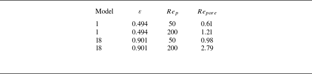
 Repore=ulocaldmin/ν
 ulocal
 dmin
 Rep
 ε

 Rep=200
 ε=0.803
 ε=0.901

 Rep=200
 x/Dp=±0.45
 ⟨Cp⟩(x)
 Rcore=[⟨Cp⟩(−0.225)−⟨Cp⟩(0.225)]/[⟨Cp⟩(−0.45)−⟨Cp⟩(0.45)]×100%

 α=0.3−0.8
 ΔCD
 (CD,porous−CD,solid)/CD,solid×100%
 ε=0.803

 CD/CD,α=0.3
 α
 Rep
 ε=0.803
 α=0.3
 Rep≥100

 Cp
 Rep=100
 ε=0.803
 α=0.3,0.5,0.8

 Rep=100
 α=0.3
 α=0.8
 m˙particle(x)/m˙0
 x/Dp
 Scross(x)
 A0
 α
 x/Dp≤0.1
 α

 Rep=200
 α=0.5
 ε=0.803

 S′
 CD⋅Rep
 ΔCD
 (CD,S′−CD,S′=3.15)/CD,S′=3.15×100%
 0%
 S′=6.34
 Rep≤20
 Rep≈50
 ≈5%

 S′
 S′=3.15
 Rep≤20
 Rep=50
 Rep≥100

 CD,f
 CD,p
 S′=6.34
 Rep=1
 Cf
 S′=3.15
 S′=6.34
 Cf
 τw
 0.5ρU∞2

 Ux∗=ux/U∞
 S′=3.15
 S′=6.34
 Ux∗=0
 Ux∗=ux/U∞

 Ux∗=ux/U∞
 Rep=200
 S′=3.15
 S′=6.34
 xw/Dp=0.01
 0.25
 0.5
 3.0
 Ux∗=0

 Rep=200
 ε=0.803
 α=0.5
 Ux∗=ux/U∞
 xw/Dp=0.01
 r⊥/Dp≤0.4
 m˙particle(x)/m˙0
 ux/U∞
 A0
 x/Dp=0
 S′
 M+
 M−
 S′
 M+
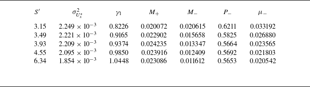
 Ux∗=ux/U∞
 ε=0.803
 α=0.5
 Rep=200
 xw/Dp=0.01
 r⊥/Dp≤0.4
 σUx∗2
 γ1
 M+,M−
 P−
 μ−
 S′

 Rep=200
 Cp
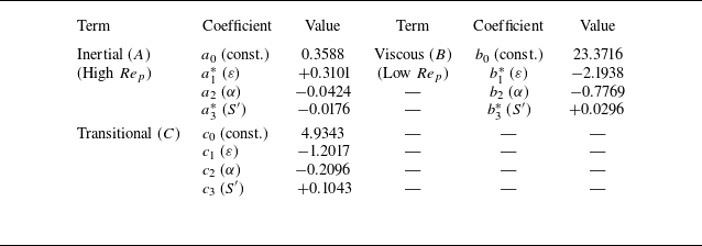
 ε≤0.901

 R2=0.9868
 MAPE=1.3%
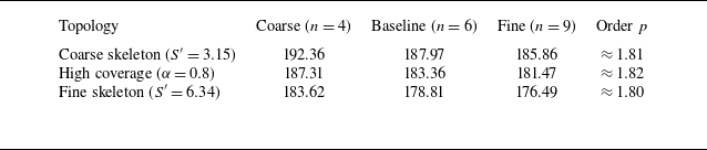
 Rep=200
 n
 dmin

 CD⋅Rep
 CD⋅Rep
 ε=0.87

 CD⋅Rep
 R2

 R2>0.99


