2 The relationship of stretcher/compressor dispersion with the refractive index of air

To calculate the impact of the refractive index of air on dispersion, we will write expressions for the grating and the total phase $\Psi$ ^[ Reference Treacy ^{6 ,} Reference Khazanov ^{7 ]}, introduced by a compressor consisting of two identical pairs of parallel gratings, in terms of the wavelength rather than of the frequency $\omega$ :

(1) $$\begin{align}\sin\theta \left(\omega \right)&=-\frac{\lambda N}{n\cos\gamma}+{\sin}\ \alpha, \end{align}$$

(2) $$\begin{align}\Psi \left(\omega \right)&=\frac{4\pi}{\lambda } nL\cos\gamma \left( \cos\theta \left(\omega \right)+ \cos\alpha \right),\end{align}$$

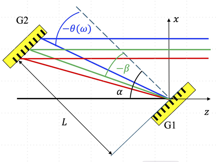
where $\lambda =2\pi c/\omega$ is the wavelength in vacuum, $\alpha$ and $\theta$ are the angles of incidence and reflection, respectively, from the first grating in the diffraction plane, $\gamma$ is the angle of incidence in the orthogonal plane and $L$ is the distance between the gratings along the normal; see Figure 1. Equation (2) can be found in Ref. [Reference Khazanov7] as well as in the classical Treacy paper^[ Reference Li, Leng and Li ^{2 ]} in a more complicated but equivalent form. The phase introduced by the stretcher is $-\Psi$ . The formal substitution

(3) $$\begin{align}L\to L/n;\kern0.72em N\to Nn\end{align}$$

Figure 1

Layout of the first compressor grating pair; the second pair is mirrored. Here, $\alpha$ and $\theta \left(\omega \right)$ are angles of incidence and reflection, respectively, and $\beta =\theta \left({\omega}_0\right)$ is the angle of reflection at central frequency ${\omega}_0$ .

Figure 1 Long description

At the lower right, grating G1 is positioned at an angle along the z axis. Multiple colored rays originate from G1, reflecting upward and leftward toward grating G2 at the upper left. G2 is also angled, mirroring G1. The rays are color-coded: blue, green, and red, representing different frequencies. The blue ray is labeled with negative theta open parenthesis omega close parenthesis, indicating the angle of reflection for frequency omega. The green ray is labeled with negative beta, representing the angle of reflection at central frequency omega sub 0. The black arc at G1 is labeled alpha, marking the angle of incidence. The distance between G1 and G2 is labeled L. The coordinate axes x and z are shown, with x vertical and z horizontal. All labels are placed at their respective geometric positions, and the layout emphasizes the angular relationships between the gratings and the rays.

transforms (1, 2) to a conventional vacuum form ( $n=1)$ .

The physical meaning of Equation (3) is that the refractive index reduces the wavelength by a factor of n, which is equivalent to a decrease in all geometric dimensions by a factor of n. Note that $\cos\gamma$ enters Equations (1) and (2) in exactly the same way as n. The difference of $\cos\gamma$ from unity means that the wave vector has a component outside the diffraction plane, that is, in the diffraction plane the wave vector is multiplied by $\cos\gamma$ and the wavelength is divided by $\cos\gamma$ , which is equivalent to an increase in all dimensions by a factor of 1/ $\cos\gamma$ . In other words, the compressors/stretchers with $n\cos\gamma = \mathrm{const}$ are equivalent to each other. By making the substitution (Equation (3)), we can generalize all the results known for vacuum. In particular

(4) $$\begin{align}{\Psi}^{\prime \prime }=-\frac{L}{n\pi {c}^2}\frac{\lambda_0^3{N}^2}{\cos\gamma {{\cos}}^3\theta \left(\omega ={\omega}_0\right)},\end{align}$$

(5) $$\begin{align}{\Psi}^{\prime \prime \prime }&=\frac{3L}{2{\pi}^2{nc}^3}\frac{\lambda_0^4{N}^2}{\cos\gamma {{\cos}}^3\theta \left(\omega ={\omega}_0\right)}\nonumber\\&\quad\times\left(1-\frac{\sin\theta \left(\omega ={\omega}_0\right)}{{{\cos}}^2\theta \left(\omega ={\omega}_0\right)}\frac{{N\lambda}_0}{n}\right),\end{align}$$

(6) $$\begin{align}\sin\theta \left(\omega ={\omega}_0\right)=-\frac{\lambda_0N}{n\cos\gamma}+\mathit{\sin}\ \alpha,\end{align}$$

where ${\lambda}_0=2\pi c/{\omega}_0$ is the central wavelength in vacuum and ${\Psi}^{\prime \prime }$ and ${\Psi}^{\prime \prime \prime }$ are the second and third derivatives of the phase (Equation (2)), respectively, with respect to frequency at $\omega ={\omega}_0$ , also referred to as group delay dispersion (GDD) and third-order dispersion (TOD). By expanding Equations (4)–(6) in a Taylor series we can find $\Delta {\Psi}^{\prime \prime }={\Psi}^{\prime \prime}\left({n}_0+\Delta n\right)-{\Psi}^{\prime \prime}\left({n}_0\right)$ and $\Delta {\Psi}^{\prime \prime \prime }={\Psi}^{\prime \prime \prime}\left({n}_0+\Delta n\right)-{\Psi}^{\prime \prime \prime}\left({n}_0\right)$ :

(7) $$\begin{align}\Delta {\Psi}^{\prime \prime }&=\Delta n\frac{L}{\pi {c}^2}\frac{\lambda_0^3{N}^2}{{\cos\gamma \cos}^3\beta}\left(1-3{\lambda}_0N\frac{\sin\beta}{{{\cos}}^2\beta}\right)\nonumber\\&=-\Delta n{\Psi}^{\prime \prime}\left(1-3{\lambda}_0N\frac{\sin\beta}{{{\cos}}^2\beta}\right),\end{align}$$

(8) $$\begin{align}\kern-6pt {\Delta \Psi}^{\prime \prime \prime }&=\frac{3L}{2{\pi}^2{c}^3}\frac{N^2{\lambda}_0^4}{{\cos\gamma \cos}^5\beta}\Delta n\nonumber\\&\quad\times\left({\mathit{\cos}}^2\beta -5 \sin\beta {\lambda}_0N+\left(1+5{\mathrm{tg}}^2\beta \right){\left({\lambda}_0N\right)}^2\right),\end{align}$$

where $\beta =\theta \left(n=1,\omega ={\omega}_0\right)$ . We took into account that ${n}_0\approx 1$ , $\left|\Delta n\right|\ll 1$ and ignored the terms of the equations with ${\Delta n}^2$ . Since β is usually $\beta <0$ , from Equations (7) and (8), it follows that $\Delta {\Psi}^{\prime \prime }>0$ and ${\Delta \Psi}^{\prime \prime \prime }>0$ , given $\Delta n>0$ , that is, an increase in pressure in the compressor introduces positive GDD and positive TOD. With a change in the refractive index $\Delta n$ in the stretcher or in the compressor, the arising $\Delta {\Psi}^{\prime \prime }$ can be zeroed by changing the distance between the gratings by $\Delta L$ . From Equations (4) and (7) we obtain the following:

(9) $$\begin{align}\Delta L=\Delta nL\left(1-3{\lambda}_0N\frac{\sin\beta}{{{\cos}}^2\beta}\right).\end{align}$$

In this case, however, the TOD (Equation (8)) also changes by ${\Psi}^{\prime \prime \prime}\Delta L/L$ and the resulting residual TOD ${\delta \Psi}^{\prime \prime \prime }=\Delta {\Psi}^{\prime \prime \prime }+{\Psi}^{\prime \prime \prime}\Delta L/L$ will be non-zero. Since ${\Psi}^{\prime \prime \prime }>0$ , from Equations (8) and (9) it follows that $\Delta {\Psi}^{\prime \prime \prime }$ and ${\Psi}^{\prime \prime \prime}\Delta L/L$ have equal signs, hence $\left|{\delta \Psi}^{\prime \prime \prime}\right|>\left|\Delta {\Psi}^{\prime \prime \prime}\right|$ , that is, aligning the length cancels out GDD, but always increases the absolute value of TOD. From Equations (5), (8) and (9) we obtain the following:

(10) $$\begin{align}{\delta \Psi}^{\prime \prime \prime }&=\frac{3L}{2{\pi}^2{c}^3}\frac{N^2{\lambda}_0^4}{\cos\gamma {{\cos}}^5\beta}\nonumber\\&\quad \times \Delta n \left(2{\mathit{\cos}}^2\beta -9 \sin\beta {\lambda}_0N+\left(1+8{\mathrm{tg}}^2\beta \right){\left({\lambda}_0N\right)}^2\right).\end{align}$$

Changes in the index of refraction $\Delta n$ can be compensated for in all orders of dispersion at once, if the angle of incidence in the plane orthogonal to the diffraction plane is changed by $\Delta \gamma$ . From Equations (4) and (7) we have the out-of-plane compressor:

(11) $$\begin{align}\Delta \gamma =\left\{\begin{array}{@{}l}\begin{array}{@{}l}\sqrt{2\Delta n}\kern0.96em \mathrm{if}\;\gamma =0\;\left(\mathrm{plane}\kern0.17em \mathrm{compressor}\right),\\ {}\;\end{array}\\ {}\; \mathrm{a}\cos\left(\frac{\cos\gamma}{1+\Delta n}\right)-\gamma \approx \Delta n\mathrm{cot}\ \gamma \kern0.24em \mathrm{if}\;\gamma \ne 0\\\quad\left(\mathrm{out}\kern0.17em \mathrm{of}\kern0.17em \mathrm{plane}\kern0.17em \mathrm{compressor}\right).\;\end{array}\right.\end{align}$$

As can be seen from Equation (11), for a flat compressor, $\Delta \gamma$ can only compensate for an increase in $n$ (only $\Delta n>0$ ). Otherwise, to satisfy the condition $n\cos\gamma = \mathrm{const}$ , $\cos\gamma$ should be increased, which is impossible when $\gamma =0$ . In what will follow, we will be interested in two cases: (i) $\Delta {\Psi}^{\prime \prime \prime }$ is neglected and only the GDD $\Delta {\Psi}^{\prime \prime }$ (Equation (7)) remains; and (ii) $\Delta {\Psi}^{\prime \prime }$ is zeroed using Equation (9) and only the TOD ${\delta \Psi}^{\prime \prime \prime }$ (Equation (10)) remains. Below, we will use the subscripts ‘2’ and ‘3’ to denote these cases. The impact of dispersion on the output pulse will be described by two parameters: $\eta,$ showing the decrease in the peak power $P\left(t={t}^{\ast}\right)$ relative to the peak power of the FTL pulse ( ${t}^{\ast }$ is the instant of time when the power is maximal, derived from the equation ${P}^{\prime}\left({t}^{\ast}\right)=0$ ), and $\tau,$ showing the pulse stretching (FWHM) ${t}_\mathrm{p}$ compared to the FTL pulse ${t}_\mathrm{FTL}$ :

(12) $$\begin{align}{\eta}_{2,3}=\frac{P_{2,3}\left(t={t}^{\ast}\right)}{P_\mathrm{FTL}\left(t=0\right)},\kern1.32em {\tau}_{2,3}=\frac{t_\mathrm{FTL}}{t_{\mathrm{p}2,3}}.\end{align}$$

Let the field spectrum have a super-Gaussian shape with index $\mu$ and spectrum halfwidth $\Delta \omega$ at the 1/e intensity level. Then the pulse peak power $P$ will be as follows:

(13) $$\begin{align}{P}_{2,3}(t)= \mathrm{const}{\left|{\int}_{-\infty}^{\infty }{e}^{-i\Delta \omega t\xi}{e}^{i{D}_{2,3}{\xi}^{2,3}}{e}^{-\frac{1}{2}{\xi}^{2\mu }}\mathrm{d}\xi \right|}^2,\end{align}$$

where ${D}_2$ and ${D}_3$ are the dimensionless GDD and TOD:

(14) $$\begin{align}{D}_2=\frac{\Delta {\Psi}^{\prime \prime }}{2}{\Delta \omega}^2,\kern1.44em {D}_3=\frac{\delta {\Psi}^{\prime \prime \prime }}{6}{\Delta \omega}^3.\end{align}$$

The physical meaning of ${D}_{2,3}$ is the difference of spectral phases at frequencies ${\omega}_0$ and ${\omega}_0\pm \Delta \omega$ . Equation (13) can be integrated exactly only for a Gaussian pulse with GDD: the pulse retains the Gaussian envelope, its duration increases by a factor of $\sqrt{1+4{D}_2^2}$ and its peak power reduces by a factor of $\sqrt{1+4{D}_2^2}$ :

(15) $$\begin{align}{\eta}_2\left(\mu =1\right)={\tau}_2\left(\mu =1\right)=\frac{1}{\sqrt{1+4{D}_2^2}}.\end{align}$$

Approximate expressions for ${\eta}_{2,3}$ can be obtained, given ${D}_{2,3}\ll 1$ , by expanding Equation (13) in a Taylor series:

(16) $$\begin{align}{\eta}_2&=\frac{1}{1+{q}_2\left(\mu \right){D}_2^2},\kern0.72em \nonumber\\{q}_2\left(\mu \right)&=\frac{\Gamma \left(\frac{5}{2\mu}\right)\Gamma \left(\frac{1}{2\mu}\right)-{\Gamma}^2\left(\frac{3}{2\mu}\right)}{\Gamma^2\left(\frac{1}{2\mu}\right)}{2}^{2/\mu },\end{align}$$

(17) $$\begin{align}{\eta}_3&=\frac{1}{1+{q}_3\left(\mu \right){D}_3^2},\kern0.6em \nonumber\\ {q}_3\left(\mu \right)&=\frac{\Gamma \left(\frac{7}{2\mu}\right)\Gamma \left(\frac{3}{2\mu}\right)-{\Gamma}^2\left(\frac{5}{2\mu}\right)}{\Gamma \left(\frac{1}{2\mu}\right)\Gamma \left(\frac{3}{2\mu}\right)}{2}^{3/\mu },\end{align}$$

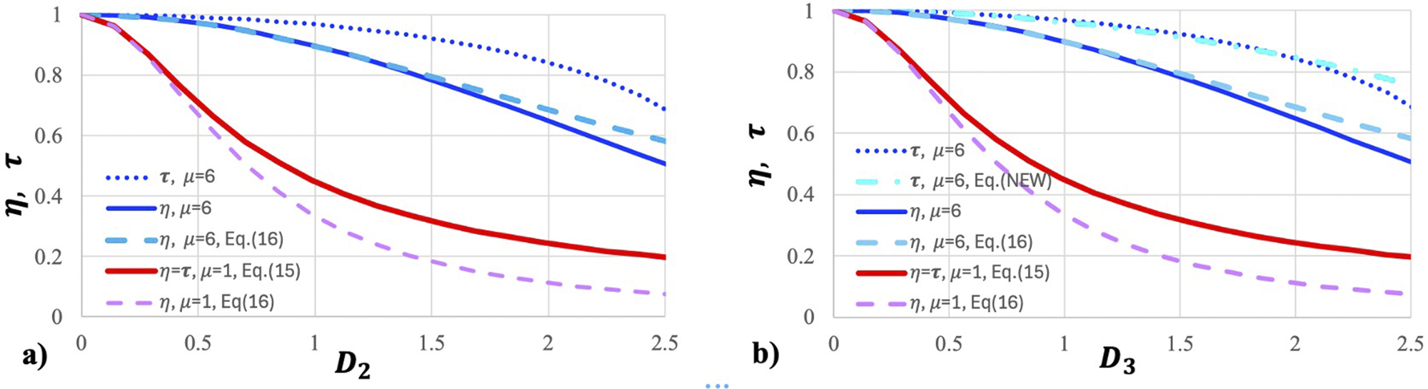
where Г is the gamma function. For ${\tau}_{2,3}$ , numerical simulation should be used. Exact (numerical and Equation (15)) and approximate (Equations (16) and (17)) dependences of $\eta$ and $\tau$ on ${D}_2$ and ${D}_3$ are plotted in Figures 2(a) and 2(b), respectively. It can be seen from Figure 2 that Equations (16) and (17) are quite accurate, even when the condition ${D}_{2,3}\ll 1$ is violated and they can be used as long as ${\eta}_{2,3}>0.75$ . The exception is ${\eta}_3$ for the Gaussian spectrum ( $\mu =1$ ). 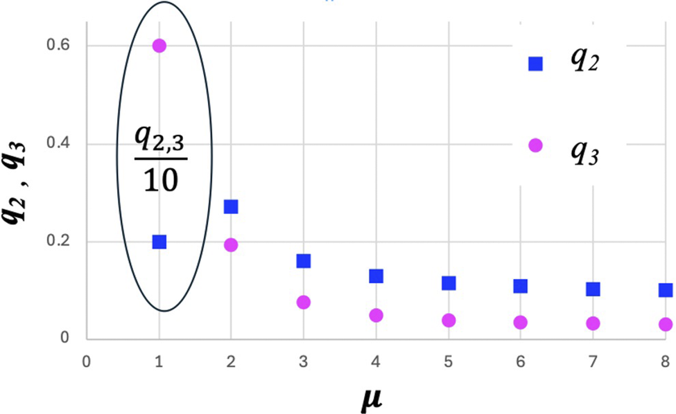The functions ${q}_{2,3}\left(\mu \right)$ are plotted in Figure 3, from which it is clear that ${q}_{2,3}\left(\mu =1\right)\gg {q}_{2,3}\left(\mu \ge 2\right)$ , that is, the Gaussian pulse is distorted much more strongly than the super-Gaussian ones; besides, ${q}_{2,3}\left(\mu \ge 4\right)\approx \mathrm{const}$ , that is, the super-Gaussian pulses differ only slightly. Further, for definiteness, we will consider $\mu =6$ . A decrease in ${\eta}_2$ and ${\tau}_2$ with increasing ${D}_2$ for the Gaussian spectrum is significantly faster than for the super-Gaussian one (compare the red and blue curves in Figure 2(a)). This is explained by the long spectrum wings, which are more sensitive to dispersion. This difference is even more pronounced for ${\eta}_3$ and ${\tau}_3$ (Figure 2(b)), since a higher dispersion order has a stronger effect on the wings of the spectrum. It should be borne in mind, however, that the peak power of an FTL pulse with a Gaussian spectrum is higher than that of a super-Gaussian one (with the same energy and the same bandwidth $\Delta \omega$ ) by $\sqrt{\pi}\mu {2}^{1-1/\mu }/\Gamma \left(0.5/\mu \right)\approx 1.65$ times. For a Gaussian pulse, ${\eta}_2={\tau}_2$ and ${\eta}_3\approx {\tau}_3$ , that is, the dispersion has approximately equal impacts on the power and pulse duration. For a super-Gaussian $\left(\mu =6\right)$ pulse at low dispersion, when the pulse power decrease is less than 25%, we have $1-{\eta}_{2,3} \approx 3\left(1-{\tau}_{2,3}\right)$ ; compare the solid blue curves with the dotted curves in Figure 2. In other words, the dispersion affects the power approximately three times more strongly than the pulse duration. For example, when the pulse is stretched by 5%, its power decreases by 15%. In experiments, the pulse duration is measured as a rule, and the factor of three must be taken into account to estimate the peak power. Another feature of the super-Gaussian spectrum is that the impacts of GDD and TOD on the pulse are the same if ${D}_3\approx 1.8{D}_2$ , while for the Gaussian spectrum, they are the same if ${D}_3\approx 0.59{D}_2$ . Note that Equations (16) and (17), Figure 2 and the conclusions made in this paragraph are valid regardless of the reasons leading to non-zero GDD and TOD. In Section 3 we will consider the effects associated with the influence of air pressure in the stretcher/compressor on ${D}_2$ and ${D}_3$ .

Figure 2

Shown are $\eta\;\mathrm{and}$ $\tau$ as a function of dimensionless GDD ${D}_2$ (a) and TOD ${D}_3$ (b). $\eta$ , solid curves are exact solutions and dashed curves are approximate solutions (Equations (16) and (17)); $\tau$ , dotted curves are exact solutions; red curves, Gaussian spectrum ( $\mu =1$ ); blue curves, super-Gaussian spectrum ( $\mu =6$ ).

Figure 2 Long description

Panel a on the left plots eta and tau on the y-axis from 0 to 1 against D sub 2 on the x-axis from 0 to 2.5. Five curves are shown: a blue dotted line for tau with mu equals 6, a solid blue line for eta with mu equals 6, a dashed light blue line for eta with mu equals 6 using Equation 16, a solid red line for eta equals tau with mu equals 1 using Equation 15, and a dashed purple line for eta with mu equals 1 using Equation 16. All curves decrease as D sub 2 increases, with tau for mu equals 6 decreasing least steeply and eta for mu equals 1 decreasing most steeply. Panel b on the right has the same y-axis and plots against D sub 3 on the x-axis. The same five curves are present, with the blue dotted line labeled tau, mu equals 6, and an additional label tau, mu equals 6, Equation NEW. The trends are similar: all curves decrease with increasing D sub 3, and the separation between curves is consistent with panel a. The legend identifies each curve by color, line style, and equation reference.

Figure 3

The ${q}_{2,3}\left(\mu \right)$ functions. Values for the Gaussian spectrum ( $\mu =1$ ) are divided by 10 for clarity.

Figure 3 Long description

The x axis is labeled mu, ranging from 0 to 8. The y axis is labeled q sub 2 comma q sub 3, ranging from 0 to 0.6. Blue squares represent q sub 2 and pink circles represent q sub 3, as indicated by the legend in the upper right. Both q sub 2 and q sub 3 have their highest values at mu equals 1, with q sub 2 near 0.2 and q sub 3 near 0.6. An oval annotation at mu equals 1 encloses both points and contains the label q sub 2 comma 3 all over 10, indicating these values are divided by 10 for clarity. For mu values greater than 1, both q sub 2 and q sub 3 decrease sharply and then remain nearly constant at lower values for increasing mu.

3 Crude effects: pressure change of the order of atmospheric pressure

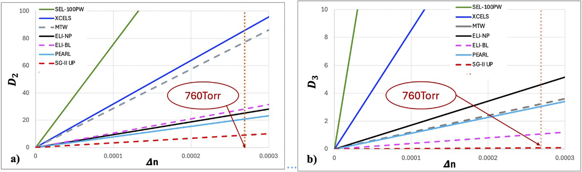
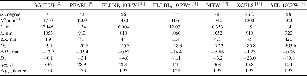
Prior to examining the influence of atmospheric pressure on $\eta$ and $\tau$ , consider cruder effects occurring when the pressure changes by an amount comparable to atmospheric pressure. In this case, $\Delta n$ is of the order of 0.000269, and for typical parameters of high-power laser facilities ${D}_2\gg 1$ , see Figure 4(a) and Table 1. Note that ${D}_2\gg 1$ for both femtosecond lasers (solid curves in Figure 4) and (sub-)picosecond neodymium lasers (dashed curves in Figure 4). In this case, the pulse shape follows the spectrum shape, and its duration at the 1/e level is ${t}_\mathrm{chirp}=2\Delta \omega \Delta {\Psi}^{\prime \prime }=4{D}_2/\Delta \omega$ , that is, a change in pressure by a value comparable to atmospheric pressure leads to stretching of the FTL pulse and a decrease in its power by many times.

Figure 4

Dimensionless GDD ${D}_2$ (a) and TOD ${D}_3$ (b) as a function of changes in the refractive index $\Delta n$ for different lasers. Detailed information on the lasers is given in Table 1.

Figure 4 Long description

Panel a on the left plots D sub 2 on the y-axis from 0 to 100 against delta n on the x-axis from 0 to 0.0003. Seven lines represent different lasers: S E L dash 100 P W (green, steepest), X C E L S (blue), M T W (black), E L I dash N P (gray dashed), E L I dash B L (magenta), P E A R L (solid red), and S G dash I I U P (red dashed, shallowest). All lines show a positive linear trend. A vertical dashed brown line and a red oval label mark delta n at approximately 0.00023, annotated as 760 Torr. Panel b on the right plots D sub 3 on the y-axis from 0 to 10 against delta n on the same x-axis range. The same seven lasers are represented with identical color and line styles. S E L dash 100 P W and X C E L S again have the steepest slopes, while S G dash I I U P and E L I dash B L are lowest. The 760 Torr marker is repeated at the same delta n value. The legend at the top right of each panel identifies the lasers by color and line style.

Table 1

Values of the parameters for different lasers at $\Delta n=-0.000269$ , assuming $\mu =6$ .

Table 1 Long description

Starting from the top row, the parameter alpha in degrees is listed as 71 for S G dash I I U P, 43 for P E A R L, 56 for E L I dash N P, 37 for E L I dash B L, 61 for M T W, 46.2 for X C E L S, and 58 for S E L dash 100 P W. The next row, N super b in 1 per millimeter, shows values of 1740, 1200, 1480, 1136, 1740, 1200, and 1320 respectively. The L parameter in meters is 2.146, 1.34, 0.904, 12.031, 0.353, 1.9, and 1.4. Lambda in nanometers is 1053, 910, 810, 1060, 1052, 910, and 920. Delta lambda in nanometers is 1.9, 41, 44, 11.4, 4.3, 75, and 120. D sub 2 values are negative: minus 9.1, minus 20.8, minus 25.3, minus 28.3, minus 77.3, minus 85.8, and minus 203.6. Delta L super c in millimeters is minus 13.7, minus 0.94, minus 0.62, minus 14.4, minus 5.86, minus 1.23, and minus 0.96. D sub 3 values are minus 0.1, minus 3.1, minus 4.6, minus 1.1, minus 3.2, minus 23.0, and minus 89.8. t sub F T L in femtoseconds is 836, 28.9, 21.4, 141, 369, 15.8, and 10.1. Delta gamma sub s in degrees is 1.33 for all except E L I dash B L, which is 0.28. Notes clarify that gamma equals 3.25 degrees for E L I dash B L, N is grove density, and Delta L is the variation of length in each grating pair, doubling if only one grating is aligned.

Notes: ^a $\gamma =3.25^{\circ}$ . ^b N is grove density. ^c $\Delta L$ is the variation of the length in each grating pair; if only one grating is aligned, then $\Delta L$ will be twice as large.

Experimenters are well aware of the fact that, if a compressor in air compresses a pulse to the FTL limit, then after evacuation $\left(\Delta n=-0.000269\right)$ the pulse is stretched substantially, and it is necessary to decrease the distance between the compressor gratings; see Equation (9). This nullifies GDD and, as noted above, increases TOD. As a result, ${D}_3$ can be significantly larger than unity, as shown in Figure 4(b) and in Table 1. In this case, decreasing the distance between the gratings is insufficient, so it is better to compensate for $\Delta n$ by changing the angle of incidence on the gratings in the plane orthogonal to the diffraction plane $\gamma$ . This method enables zeroing not only the third but also all orders of dispersion. From Equation (11) it is clear that, for a plane compressor ( $\gamma =0$ ), there is no way to compensate for $\Delta n<0$ by changing the angle $\gamma$ in the compressor. However, this can be done by changing the angle $\gamma$ in the stretcher, since the sign of the dispersion in the stretcher is opposite and, instead of Equation (11), for ${\Delta \gamma}_\mathrm{s}$ we obtain ${\Delta \gamma}_\mathrm{s}=\sqrt{-2\Delta n}={1.33}^{\mathrm{o}}$ (for a plane compressor). Note that the specified value of ${\Delta \gamma}_\mathrm{s}$ is a universal quantity, independent of the compressor and radiation parameters. For an out-of-plane compressor, ${\Delta \gamma}_\mathrm{s}$ is significantly smaller: for ${\gamma}_\mathrm{s}={3.25}^{\mathrm{o}}$ , from Equation (11) we obtain ${\Delta \gamma}_\mathrm{s}={0.284}^{\mathrm{o}}\kern0.24em \mathrm{and}\kern0.17em \mathrm{for}\kern0.24em {\gamma}_\mathrm{s}={10}^{\mathrm{o}},\kern0.36em {\Delta \gamma}_\mathrm{s}={0.088}^{\mathrm{o}}$ . It is worth saying that ${\Delta \gamma}_\mathrm{s}$ should be the same (including the sign) for the first and third reflections from the stretcher grating. In other words, both the roof-mirror placed after two reflections and the input mirror should be rotated by the angle ${\Delta \gamma}_\mathrm{s}/2$ . Such a tuning guarantees compensation of all orders of dispersion and absence of unwanted consequences, such as spatial or angular chirp, beam pointing deviation and wavefront distortions. If the stretcher is located in a gas chamber, then a 760-Torr pressure decrease in it also nullifies all orders of dispersion caused by compressor evacuation, without mechanical distortions.

The effect of multiple pulse stretching with pressure changes can be not only parasitic but also useful. In Ref. [Reference Begishev, Bromage and Zuegel5] it was used to control the pulse duration over a wide range without mechanical distortions for a multiterawatt laser^[ Reference Begishev, Bagnoud, Bahk, Bittle, Brent, Cuffney, Dorrer, Froula, Haberberger, Mileham, Nilson, Okishev, Shaw, Shoup, Stillman, Stoeckl, Turnbull, Wager, Zuegel and Bromage ^{12 ]}, and the intensity autocorrelation functions (ACFs) were measured for different pressures. For ${D}_2\gg 1$ , the pulse shape follows the shape of the spectrum, which is close to flat-top. The ACF of the flat-top pulse has a triangular shape with a duration at half maximum equal to ${t}_\mathrm{chirp}=4{D}_2/\Delta \omega$ . For the compressor geometry described in Ref. 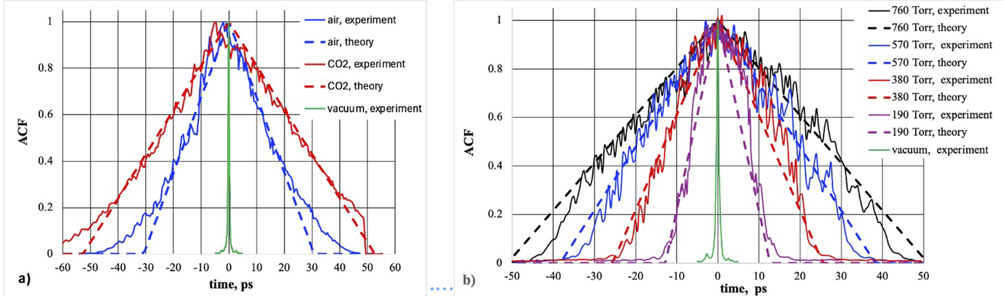[Reference Begishev, Bagnoud, Bahk, Bittle, Brent, Cuffney, Dorrer, Froula, Haberberger, Mileham, Nilson, Okishev, Shaw, Shoup, Stillman, Stoeckl, Turnbull, Wager, Zuegel and Bromage12], ${D}_2$ strongly depends on the angle of incidence $\alpha$ on the first grating of the compressor. In Ref. [Reference Begishev, Bromage and Zuegel5], this angle is given for a 61° stretcher; in the compressor, it is close to this value, although not necessarily equal to it. For a quantitative comparison with the experiment, we used α as a fitting parameter and ${D}_2$ was calculated using Equation (14). Good agreement with the experiments was obtained with $\alpha =60.6^{\circ}$ and $\alpha =61.7^{\circ}$ for the data from Ref. [Reference Begishev, Bromage and Zuegel5]; see Figures 5(a) and 5(b).

Figure 5

Comparison of theoretical (dashed curves) and experimental (solid curves) autocorrelation function measured in Ref. [Reference Begishev, Bromage and Zuegel5] for air and CO₂ at atmospheric pressure (а) and for air at different values of pressure (b).

Figure 5 Long description

Panel a on the left has x-axis labeled time, p s from minus 60 to 60 and y-axis labeled A C F from 0 to 1. Five lines are shown: solid blue for air experiment, dashed blue for air theory, solid red for C O sub 2 experiment, dashed red for C O sub 2 theory, and solid green for vacuum experiment. All lines peak at zero time, with air and C O sub 2 curves broader than vacuum. Theoretical curves are smoother and slightly narrower than experimental. Panel b on the right has the same axes but time, p s ranges from minus 50 to 50. Eight lines are shown: solid black for 760 Torr experiment, dashed black for 760 Torr theory, solid blue for 570 Torr experiment, dashed blue for 570 Torr theory, solid red for 380 Torr experiment, dashed red for 380 Torr theory, solid magenta for 190 Torr experiment, dashed magenta for 190 Torr theory, and solid green for vacuum experiment. As pressure decreases from 760 to 190 Torr, both experimental and theoretical curves become narrower. The vacuum curve is the narrowest and tallest. Theoretical lines are always smoother than experimental.

4 Fine effects: atmospheric pressure impact

The compressor of high-power lasers is located in vacuum to eliminate nonlinear effects in the air. The stretcher is usually located in air. With small pressure changes (of about 10 Torr), a change in the GDD is significantly less than during evacuation; it is already commensurate with unity, as shown in Figure 4(a). In this case, it is convenient to find ${\eta}_{2,3}$ from the approximate formulas (Equations (16) and (17)). Taking into account $\Delta n=\frac{\mathrm{d}n}{\mathrm{d}p}\Delta p$ , from Equations (7), (10), (14), (16) and (17) it is easy to find the value of the change in the atmospheric pressure ${\Delta p}_{2,3}$ leading to a power drop to a given ${\eta}_{2,3}$ level:

(18) $$\begin{align}\left|{\Delta p}_2\right|&=\sqrt{\frac{1-{\eta}_2}{q_2\left(\nu \right)}}\frac{\pi {c}^2}{L{\lambda}_0^3{N}^2}\frac{{\cos\gamma \cos}^5\beta }{\frac{\mathrm{d}n}{\mathrm{d}p}{\Delta \omega}^2\left({{\cos}}^2\beta -3{\lambda}_0 N\sin\beta \right)},\end{align}$$

(19) $$\begin{align}\left|{\Delta p}_3\right|&=\sqrt{\frac{1-{\eta}_3}{q_3\left(\mu \right)}}\frac{4{\pi}^2{c}^3}{\frac{\mathrm{d}n}{\mathrm{d}p}\Delta {\omega}^3L{N}^2{\lambda}_0^4}\nonumber\\&\quad\times\frac{\cos\gamma {\mathit{\cos}}^5\beta }{2{\mathit{\cos}}^2\beta -9 \sin\beta {\lambda}_0N+\left(1+8{\mathrm{tg}}^2\beta \right){\left({\lambda}_0N\right)}^2}.\end{align}$$

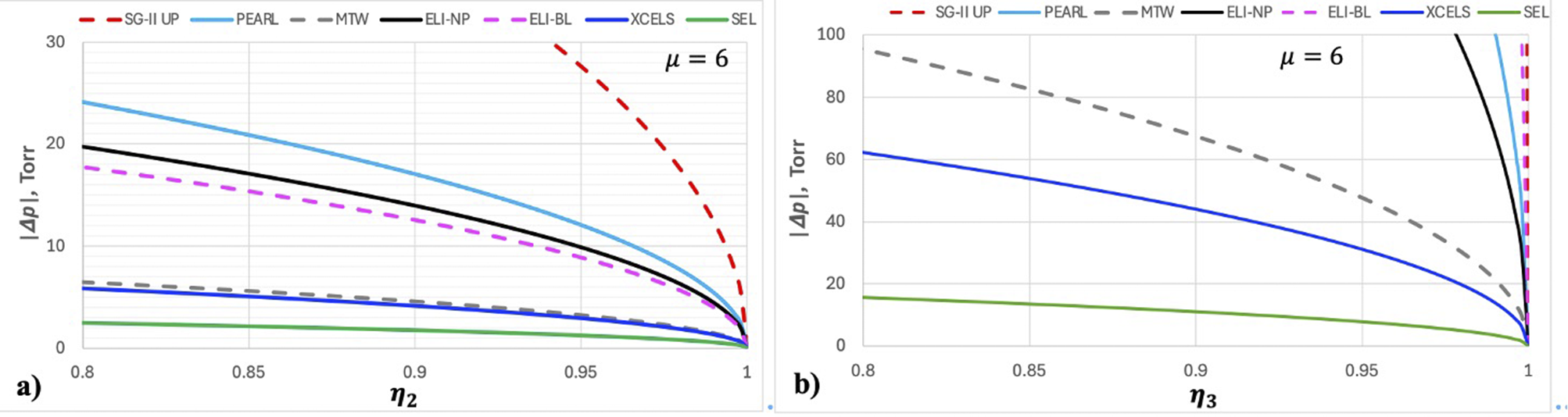
The dependence of $\left|\Delta p\right|$ on ${\eta}_{2,3}$ for different lasers is shown in Figure 6. From Figure 6(b) it is clear that, given that the change in atmospheric pressure is compensated for by aligning the distance between the gratings, the decrease in power can be neglected, except for the SEL-100 PW facility, for which even in this case the power will decrease by 20% with a pressure change of 20 Torr. Such aligning may be not needed only for PEARL and SG-II UP, whereas in the other considered lasers the power drops by 20% for $\left|{\Delta p}_2\right|$ from 3 Torr (SEL-100 PW) to 23 Torr (ELI-NP); see Figure 6(a). Typically, climate control in the laboratory excludes draught, which may induce fast pressure changes. In this case, the characteristic time of atmospheric pressure change is hours and the pulse duration increase and peak power decrease may be eliminated by a feedback system, if available. If not, the compressor should be aligned manually. To avoid alignment, it is necessary either to stabilize the atmospheric pressure in the laboratory or to place the stretcher in an evacuated chamber, as, for example, in Ref. [Reference Vyhlídka, Trojek, Kramer, Peceli, Batysta, Bartoníček, Hubáček, Borger, Antipenkov, Gaul, Ditmire and Rus11].

Figure 6

Change in the atmospheric pressure $\left|\Delta p\right|$ leading to a power drop to a given ${\eta}_2$ (Equation (18)) (а) and ${\eta}_3$ (Equation (19)) (b) for different lasers. Detailed information on the lasers is given in Table 1.

Figure 6 Long description

Panel a on the left plots absolute atmospheric pressure change in Torr on the y-axis from 0 to 30 against eta sub 2 on the x-axis from 0.8 to 1. Seven lines represent different lasers: S G dash I I U P (red dashed) starts highest and decreases steeply, PEARL (blue solid) and XCELS (light blue solid) are next, MTW (gray solid) and ELI dash BL (magenta dashed) are intermediate, ELI dash N P (black solid) is slightly higher, and SEL (green solid) remains lowest and nearly flat. All lines converge as eta sub 2 approaches 1. Panel b on the right plots the same y-axis but up to 100 Torr against eta sub 3 from 0.8 to 1. S G dash I I U P (red dashed) is absent, MTW (gray dashed) starts highest, PEARL (blue solid) and XCELS (light blue solid) are next, ELI dash N P (black solid) and ELI dash BL (magenta dashed) are clustered at the right, and SEL (green solid) remains lowest and nearly flat. All lines converge as eta sub 3 approaches 1. The legend at the top identifies each laser by color and line style. The label mu equals 6 appears in both panels.

In the latter case, it is possible not only to avoid the negative effects that occur during compressor evacuation (see Section 3) and changes in atmospheric pressure but also to control the dispersion. If it is sufficient to control only ${D}_2$ , this can be done without any mechanical distortions at all, only by changing the pressure $\Delta p$ (or by mixing air with СО₂). Here, ${D}_2$ depends linearly on pressure, and the proportionality factor can be easily found from Equations (7) and (14). Furthermore, ${D}_2$ can be smoothly varied in this way over a wide range. Changing the air pressure by 1 Torr leads to a change in ${D}_2$ by a value of from 0.0119 for SG-II UP to 0.268 for SEL-100 PW, which is quite sufficient for smooth and well-controlled dispersion management; see Figure 2(a). The GDD and TOD may be controlled by the pressure and the distance between the gratings, thereby avoiding angular aligning. For the required values of ${D}_2$ and ${D}_3$ , by substituting $L+\Delta L$ for L in Equations (7) and (10) and solving the system of two linear equations, we can easily find $\Delta p$ and $\Delta L$ . Finally, GDD, TOD and the fourth-order dispersion can be controlled using $\Delta p$ , $\Delta L$ and changing the angle of incidence $\Delta \alpha$ . Furthermore, by placing the stretcher in the chamber we can eliminate the spatial inhomogeneity of n due to airflows, which leads to space–time coupling effects that negatively affect the pulse intensity at the focal point.