1 Introduction
Large-scale coherent structures, or wavepackets, in turbulent jets have been subjected to intensive study, largely because of their role in the noise production of aircraft engines (Jordan & Colonius Reference Jordan and Colonius2013). In the wake of early experimental observations by Mollo-Christensen (Reference Mollo-Christensen1963) and Crow & Champagne (Reference Crow and Champagne1971), theorists developed a number of instability wave theories to model these structures. Examples include parallel and weakly non-parallel linear stability analyses by Michalke (Reference Michalke1971, Reference Michalke1984) and Crighton & Gaster (Reference Crighton and Gaster1976), respectively. The use of parabolized stability equations (PSEs) to model wavepackets was pioneered by Yen & Messersmith (Reference Yen and Messersmith1998). Later, Gudmundsson & Colonius (Reference Gudmundsson and Colonius2011) and Cavalieri et al. (Reference Cavalieri, Rodríguez, Jordan, Colonius and Gervais2013) found close agreement between their PSE solutions and the leading spectral proper orthogonal modes (POD) obtained from experiment. An important implication of their work is that linear analyses of the turbulent mean provide approximations to the statistically averaged coherent structures.
The capability of linear global modes to capture both the hydrodynamic near-field as well as the far-field acoustics was demonstrated by Nichols & Lele (Reference Nichols and Lele2011) for the example of a cold
 $M=2.5$
laminar jet. Apart from the Kelvin–Helmholtz-type (K–H) shear-layer instability, the global modes contained upstream-travelling acoustic waves related to modes predicted from the local analysis of Tam & Hu (Reference Tam and Hu1989). In some cases, these upstream-travelling waves may lead to resonance mechanisms. An example occurs in impinging jets, where feedback between K–H wavepackets and acoustic modes may lead to tones in the pressure field (Tam & Ahuja Reference Tam and Ahuja1990). Although some tones have also been observed in the near field of free high-subsonic jets (Suzuki & Colonius Reference Suzuki and Colonius2006), their relation to a feedback mechanism has not been established.
The present paper considers the global stability of turbulent jets at high-subsonic speeds, and provides a thorough comparison with experimentally validated large eddy simulation data. We first show that large-scale coherent structures are a pertinent feature of fully turbulent jets, and persist over a wide range of frequencies and azimuthal wavenumbers. Spectral POD and cross-spectral density estimates are used to educe these structures from the large eddy simulation (LES) data. Besides the well-known K–H instability waves in the shear layer, acoustic waves that are trapped inside the potential core are found. In particular, we investigate a novel class of resonant acoustic modes, and show that they are a pertinent feature of high-subsonic turbulent jets. Throughout the study, emphasis is placed on the mutual comparison of the educed structures and linear global modes.
The paper is organized as follows. Our methodology is introduced in § 2, including an overview of the LES database, the global stability approach and the coherent structure eduction techniques. The identified coherent structures are discussed in § 3 and compared to linear global modes in § 4. A special class of resonant trapped acoustic waves is investigated in detail in § 5. A dispersion relation of the latter modes is reconstructed from the global modes and compared to the empirical dispersion relation obtained from the LES. Our findings are summarized in § 6. Details on the numerical aspects can be found in appendices A–D.
2 Methodology
2.1 Turbulent jet database
The present study builds on the LES of a
 $M_{j}=0.9$
,
 $Re\approx 10^{6}$
turbulent jet, performed using the compressible flow solver ‘Charles’ developed at Cascade Technologies (Brès et al.
Reference Brès, Ham, Nichols and Lele2017). By
 $M_{j}=U_{j}/a_{j}$
we denote the Mach number, and by
 $Re=\unicode[STIX]{x1D70C}_{j}U_{j}D/\unicode[STIX]{x1D707}_{j}$
the Reynolds number, respectively. The jet is isothermal with
 $T_{j}/T_{\infty }=1$
. The subscripts
 $j$
and
 $\infty$
denote jet and free-stream (ambient) quantities,
 $a$
speed of sound,
 $\unicode[STIX]{x1D70C}$
density,
 $D$
nozzle diameter,
 $\unicode[STIX]{x1D707}$
dynamic viscosity,
 $T$
temperature and
 $U_{j}$
the centreline jet velocity at the nozzle exit, respectively. We denote by
 $\boldsymbol{q}(\boldsymbol{x},t)=[\unicode[STIX]{x1D70C}u_{x}u_{r}u_{\unicode[STIX]{x1D703}}T]^{\text{T}}(x,r,\unicode[STIX]{x1D703},t)$
the vector of dependent variables, with
 $u_{x}$
,
 $u_{r}$
,
 $u_{\unicode[STIX]{x1D703}}$
as the cylindrical velocity components in the streamwise
 $x$
, radial
 $r$
and azimuthal direction
 $\unicode[STIX]{x1D703}$
, respectively. All variables are non-dimensionalized by their centreline nozzle value, pressure by
 $\unicode[STIX]{x1D70C}_{j}U_{j}^{2}$
, lengths by
 $D$
and time by
 $D/U_{j}$
. The frequency is represented by the dimensionless Strouhal number
 $St=\unicode[STIX]{x1D714}/(2\unicode[STIX]{x03C0}M_{j})$
, where
 $\unicode[STIX]{x1D714}$
is the angular frequency. The LES domain contains a convergent-straight nozzle. Its turbulent exit characteristics match the conditions of the tripped exit boundary layer of its experimental counterpart thanks to the introduction of synthetic turbulence combined with a wall model. The reader is referred to Brès et al. (Reference Brès, Jordan, Colonius, Le Rallic, Jaunet and Lele2014, Reference Brès, Jaunet, Le Rallic, Jordan, Colonius and Lele2015, Reference Brès, Jaunet, Le Rallic, Jordan, Towne, Schmidt, Colonius, Cavalieri and Lele2016) for further details and the extensive experimental validation, and to Bodony & Lele (Reference Bodony and Lele2008) for an overview of the use of LES in jet noise prediction. The database used in this work consists of
 $10^{4}$
snapshots, temporally separated by
 $\unicode[STIX]{x0394}tc_{\infty }/D=0.2$
and interpolated on a
 $656\times 138\times 128$
cylindrical grid spanning
 $x,r,\unicode[STIX]{x1D703}\in [0,30]\times [0,6]\times [0,2\unicode[STIX]{x03C0}]$
i.e. excluding the nozzle. Data sampled in a smaller domain but at a higher rate of
 $\unicode[STIX]{x0394}tc_{\infty }/D=0.05$
are used only to construct the frequency–wavenumber diagrams shown in figures 11–13.
The usual Reynolds decomposition
 $$\begin{eqnarray}q(\boldsymbol{x},t)=\bar{q}(\boldsymbol{x})+q^{\prime }(\boldsymbol{x},t)\end{eqnarray}$$
of any given flow quantity
 $q(\boldsymbol{x},t)$
into a long-time mean
 $\bar{q}(\boldsymbol{x})$
and a fluctuation part
 $q^{\prime }(\boldsymbol{x},t)$
is adopted. The visualization of the streamwise perturbation velocity
 $u_{x}^{\prime }$
presented in figure 1 highlights the wide range of spatial and temporal scales occurring in the turbulent jet. Two lines of constant mean streamwise velocity
 $\bar{u}_{x}=0.95$
and 0.05 delineate the potential core and the radial extent of the jet. The same isolines at
 $\bar{u}_{x}=0.95$
and 0.05 are reproduced in all later figures that show the streamwise-radial plane.
Instantaneous streamwise perturbation velocity (

 $-0.5\leqslant u_{x}^{\prime }/\Vert u_{x}^{\prime }\Vert _{\infty }\leqslant 0.5$
) and streamwise mean velocity (—— (red),
 $\bar{u}_{x}=0.95$
; – – – (red),
 $\bar{u}_{x}=0.05$
) of the LES: (a) streamwise plane and computational domain
 $\unicode[STIX]{x1D6FA}$
used for the linear stability analysis (—— (blue), solution domain; – – – (blue), sponge region) and (b–e) transverse planes at
 $x=2,5,10$
and 15, respectively.

2.2 Global stability analysis
In what follows, we adopt the notion that ‘turbulence establishes an equivalent laminar flow profile as far as large-scale modes are concerned’ (Crighton & Gaster Reference Crighton and Gaster1976), implying that the mean Reynolds stresses are implicitly accounted for in the turbulent mean flow that we draw from the LES. The fluctuating Reynolds stresses, to the extent that they are significant at a given frequency, are assumed to act as a disorganized forcing on the large-scale structures. This viewpoint has been adopted in a number of studies exploiting resolvent analysis (e.g. Farrell & Ioannou Reference Farrell and Ioannou1993; McKeon & Sharma Reference McKeon and Sharma2010; Towne et al.
Reference Towne, Colonius, Jordan, Cavalieri and Brès2015), and is supported by previous studies comparing parabolized stability equation models for the coherent wavepackets in jets to microphone and particle image velocimetry (PIV) data (Gudmundsson & Colonius Reference Gudmundsson and Colonius2011; Cavalieri et al.
Reference Cavalieri, Rodríguez, Jordan, Colonius and Gervais2013). In the present case, in advance of a full resolvent analysis of the jet, we further neglect this stochastic forcing and instead catalogue the unforced behaviour of the linear modes of the turbulent mean flow field. Neglecting nonlinear interaction terms in the governing equations, and assuming perturbations of the normal-mode form with azimuthal wavenumber
 $m$
 $$\begin{eqnarray}q^{\prime }(x,r,\unicode[STIX]{x1D703},t)=\hat{q}_{m}(x,r)\text{e}^{\text{i}(m\unicode[STIX]{x1D703}-\unicode[STIX]{x1D714}t)},\end{eqnarray}$$
yields the usual eigenvalue problem
 $$\begin{eqnarray}(\text{i}\unicode[STIX]{x1D714}+{\mathcal{L}}_{m})\hat{q}_{m}=0,\end{eqnarray}$$
where
 ${\mathcal{L}}_{m}={\mathcal{L}}_{m}(\bar{q})$
is the global linear stability operator based on the mean flow. In our case,
 ${\mathcal{L}}_{m}$
represents the system of the linearized compressible continuity, Navier–Stokes and energy equations for an ideal gas in cylindrical coordinates. The radial streamwise plane is discretized by fourth-order summation by parts finite differences developed by Mattsson & Nordström (Reference Mattsson and Nordström2004), and the polar singularity is treated as in Mohseni & Colonius (Reference Mohseni and Colonius2000). Non-reflecting boundary conditions are enforced using a sponge region.
The resulting discrete generalized eigenvalue problem reads
 $$\begin{eqnarray}(\unicode[STIX]{x1D714}\unicode[STIX]{x1D644}+\unicode[STIX]{x1D647}_{m})\hat{\boldsymbol{q}}_{m}=0,\end{eqnarray}$$
where
 $\unicode[STIX]{x1D644}$
is the identity matrix and
 $\hat{\boldsymbol{q}}_{m}=[\hat{\unicode[STIX]{x1D70C}}_{m}\;\hat{u} _{x,m}\;\hat{u} _{r,m}\;\hat{u} _{\unicode[STIX]{x1D703},m}\;\hat{T}_{m}]^{\text{T}}(x,r)$
the solution vector of primitive variables. It is solved using a shift-and-invert Arnoldi algorithm. The corresponding adjoint global stability eigenvalue problem
 $$\begin{eqnarray}(\unicode[STIX]{x1D714}^{\ast }\unicode[STIX]{x1D644}+\unicode[STIX]{x1D647}_{m}^{\dagger })\hat{\boldsymbol{q}}_{m}^{\dagger }=0,\end{eqnarray}$$
is defined through the definition of the adjoint operator,
 $\langle \unicode[STIX]{x1D647}_{m}\hat{\boldsymbol{q}}_{m},\hat{\boldsymbol{q}}_{m}^{\dagger }\rangle _{E}=\langle \hat{\boldsymbol{q}}_{m},\unicode[STIX]{x1D647}_{m}^{\dagger }\hat{\boldsymbol{q}}_{m}^{\dagger }\rangle _{E}$
in the energy norm for a compressible gas
 $$\begin{eqnarray}\langle q,q\rangle _{E}=\iiint q^{H}\text{diag}\left(\frac{\overline{T}}{\unicode[STIX]{x1D6FE}\overline{\unicode[STIX]{x1D70C}}M_{j}^{2}},\overline{\unicode[STIX]{x1D70C}},\overline{\unicode[STIX]{x1D70C}},\overline{\unicode[STIX]{x1D70C}},\frac{\overline{\unicode[STIX]{x1D70C}}}{\unicode[STIX]{x1D6FE}(\unicode[STIX]{x1D6FE}-1)\overline{T}M_{j}^{2}}\right)qr\,\text{d}x\,\text{d}r\,\text{d}\unicode[STIX]{x1D703}=q^{H}\unicode[STIX]{x1D652}q,\end{eqnarray}$$
as derived by Chu (Reference Chu1965). Here,
 $\unicode[STIX]{x1D652}$
is the discretized weight matrix,
 $\unicode[STIX]{x1D6FE}$
the specific heat ratio and
 $(\text{}^{\ast })$
indicates the scalar complex conjugate, or the conjugate transpose for vectors and matrices, respectively. For its ease of implementation, we chose the discrete-adjoint framework (Chandler et al.
Reference Chandler, Juniper, Nichols and Schmid2012). The adjoint eigenvectors
 $\hat{\boldsymbol{q}}_{m}^{\dagger }$
are normalized according to
 $\langle \hat{\boldsymbol{q}}_{m}^{\dagger },\hat{\boldsymbol{q}}_{m}\rangle _{E}=1$
.
Direct and adjoint global modes are calculated in the computational domain
 $\unicode[STIX]{x1D6FA}$
outlined in figure 1(a) for a Reynolds number of
 $Re=10^{5}$
. Details on the grid resolution, the sponge layer and the spatial discretization can be found in appendix A. The influence of the sponge on the trapped acoustic modes is discussed in appendix B and the effect of domain truncation is discussed in appendix C. Our choice to conduct a linear stability analysis of the turbulent mean flow is motivated, and the effect of the of Reynolds number on the global spectra is addressed in detail, in appendix D.
2.3 Coherent structure eduction techniques
As the jet is periodic in the azimuthal direction, the fluctuation field can be decomposed into Fourier modes of azimuthal wavenumber
 $m$
as
 $$\begin{eqnarray}q^{\prime }(x,r,\unicode[STIX]{x1D703},t)=\mathop{\sum }_{m}\tilde{q}_{m}(x,r,t)\text{e}^{\text{i}m\unicode[STIX]{x1D703}},\end{eqnarray}$$
and further, under the assumption of statistical stationarity in time, into spatio-temporal modes
 $$\begin{eqnarray}\tilde{q}_{m}(x,r,t)=\mathop{\sum }_{\unicode[STIX]{x1D714}}\tilde{\tilde{q}}_{m,\unicode[STIX]{x1D714}}(x,r)\text{e}^{\text{i}m\unicode[STIX]{x1D703}}\text{e}^{\text{i}\unicode[STIX]{x1D714}t}\end{eqnarray}$$
of angular frequency
 $\unicode[STIX]{x1D714}$
.
Spectra are estimated using Welch’s method by partitioning the time series into sequences of 256 snapshots with an overlap of 50 %. This partition is found to be a good compromise between a sufficiently high discrete frequency spacing and a sufficiently high number
 $N_{b}=78$
of statistically independent realizations, or blocks. The power spectral density (PSD) for a given frequency and azimuthal wavenumber is then estimated as
 $$\begin{eqnarray}\bar{P}_{qq}(x,r)=\frac{1}{N_{b}}\mathop{\sum }_{n=1}^{N_{b}}|\tilde{\tilde{q}}_{m,\unicode[STIX]{x1D714}}^{(n)}(x,r)|^{2},\end{eqnarray}$$
and the cross-spectral density (CSD) between any point
 $(x,r)$
in the domain and a specific location
 $(x_{0},r_{0})$
as
 $$\begin{eqnarray}\bar{C}_{qq}(x,r,x_{0},r_{0})=\frac{1}{N_{b}}\mathop{\sum }_{n=1}^{N_{b}}\tilde{\tilde{q}}_{m,\unicode[STIX]{x1D714}}^{(n)}(x,r)\tilde{\tilde{q}}_{m,\unicode[STIX]{x1D714}}^{\ast (n)}(x_{0},r_{0}).\end{eqnarray}$$
Alternatively, frequency domain or spectral POD can be applied to extract coherent structures from the column matrix of short-time Fourier realizations
 $\unicode[STIX]{x1D64C}_{m,\unicode[STIX]{x1D714}}=[\tilde{\tilde{q}}_{m,\unicode[STIX]{x1D714}}^{(1)},\tilde{\tilde{q}}_{m,\unicode[STIX]{x1D714}}^{(2)},\ldots ,\tilde{\tilde{q}}_{m,\unicode[STIX]{x1D714}}^{(N_{b})}]$
through the solution of the eigenvalue problem
 $$\begin{eqnarray}\unicode[STIX]{x1D733}^{\ast }\unicode[STIX]{x1D64C}_{m,\unicode[STIX]{x1D714}}^{\ast }\unicode[STIX]{x1D652}\unicode[STIX]{x1D64C}_{m,\unicode[STIX]{x1D714}}\unicode[STIX]{x1D733}=\unicode[STIX]{x1D726},\end{eqnarray}$$
where
 $\unicode[STIX]{x1D64C}_{m,\unicode[STIX]{x1D714}}\unicode[STIX]{x1D733}$
is the column matrix of orthonormal spectral POD modes whose energy is given by the eigenvalues along the diagonal of
 $\unicode[STIX]{x1D726}$
. The spectral POD modes optimally represent the data in terms of the energy norm induced by the inner product
 $\langle q,q\rangle _{E}$
(2.6) at each given frequency. As an example, CSD and spectral POD are employed to extract the coherent portion of the flow field in figure 2. Figure 2(a–d) shows the first two realizations in the ensemble of short-time Fourier decompositions used for the spectral estimation.
Spectral decomposition and coherent feature extraction for
 $m=0$
,
 $St\approx 0.5$
(

 $\pm 0.5$
of the maximum value): (a–d) the first two realizations of the 256 snapshot based Fourier decomposition; (e–h) CSD using different correlation points
 $(x_{0},r_{0})$
; (i,j) leading POD mode estimates. The pressure and streamwise velocity component are shown in the left and right column, respectively. The CSD correlates each point of the flow field with a location
 $(x_{0},r_{0})$
marked by ‘
 $+$
’, and the POD is based on the volume weighted 2-norm.
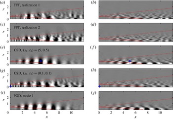
The K–H instability and a monochromatic high-wavenumber fluctuation in the potential core are observed in both realizations. We will show later that the wave inside the core is acoustic and propagates upstream with a negative phase velocity. In our parallel investigation, Towne et al. (Reference Towne, Cavalieri, Jordan, Colonius, Schmidt, Jaunet and Brès2017) show that this latter disturbance is an acoustic wave that experiences the shear layer as an annual duct and is therefore trapped within the potential core. The CSD is particularly useful to identify spatially correlated portions of the fluctuation field in a specific region. The K–H instability, for example, is accentuated in figure 2(e,f) for a correlation location
 $(x_{0},r_{0})=(5,0.5)$
within the shear layer. Similarly, a location
 $(x_{0},r_{0})=(0.1,0.1)$
close to the nozzle centreline in figure 2(g,h) highlights the acoustic wave. It also shows that the fluctuations in the core are correlated with the shear-layer instability. The K–H wavepacket is identified by POD as the most energetic structure based on a global pressure 2-norm in figure 2(i,j).
The comparison of the different eduction techniques leads to the following choices for the remainder of this paper. POD estimates are best suited to distil the average K–H wavepacket as it represents the most energetic coherent structure. Acoustic waves inside the potential core are most unambiguously educed via a CSD of the pressure field with respect to a point near the inlet and close to the jet axis.
3 Coherent features of the turbulent jet
The two families of coherent instabilities of interest for the present investigation are the K–H wavepackets in the shear layer and the trapped acoustic waves in the potential core. Their frequency and azimuthal wavenumber dependence is addressed in §§ 3.1 and 3.2, respectively.
3.1 Kelvin–Helmholtz wavepackets
In figure 3, the K–H wavepacket is identified as the most energetic coherent structure of the LES via POD for
 $m=0$
(a,c,e,g,i,k) and
 $m=4$
(b,d,f,h,j,l) over a range of frequencies. The wavepackets are characterized by a monotonic increase in wavenumber and a simultaneous decrease of their streamwise support with frequency. Their phase speed is
 $c_{ph}\approx 0.8U_{j}$
in all cases and was estimated as explained below in the context of figure 8.
Spectral estimation of pressure POD modes (

 $-0.25\leqslant \unicode[STIX]{x1D6F9}_{p}/\Vert \unicode[STIX]{x1D6F9}_{p}\Vert _{\infty }\leqslant 0.25$
) for different Strouhal numbers: (a,c,e,g,i,k)
 $m=0$
; (b,d,f,h,j,l)
 $m=4$
.

The K–H instability amplifies to the end of the spatially unstable region of the mean flow and subsequently decays. For intermediate frequencies, the support of the resulting wavepacket extends from the nozzle up to approximately the end of the potential core, and PSE (Gudmundsson & Colonius Reference Gudmundsson and Colonius2011; Cavalieri et al. Reference Cavalieri, Rodríguez, Jordan, Colonius and Gervais2013; Baqui et al. Reference Baqui, Agarwal, Cavalieri and Sinayoko2015) and linearized Euler solutions (Baqui et al. Reference Baqui, Agarwal, Cavalieri and Sinayoko2015) were found to be in good agreement with measured or simulated structures. Recent studies based on the resolvent operator (Garnaud et al. Reference Garnaud, Lesshafft, Schmid and Huerre2013b ; Jeun, Nichols & Jovanović Reference Jeun, Nichols and Jovanović2016; Semeraro et al. Reference Semeraro, Lesshafft, Jaunet and Jordan2016; Qadri & Schmid Reference Qadri and Schmid2017; Tissot et al. Reference Tissot, Zhang, Lajús, Cavalieri and Jordan2017) furthermore showed that, due to the non-normal nature of the operator, the K–H instability can be forced efficiently through the Orr mechanism. In addition to the dominant K–H wavepacket, the trapped-wave component in the potential core is also clearly visible in figure 3(c).
3.2 Trapped acoustic waves
Trapped acoustic waves are extracted by use of CSD in figure 4 for the same Strouhal numbers considered in figure 3 above. The fluctuations inside the potential core are strongly correlated with the K–H wave in all cases. Inside the potential core, acoustic waves are observed for some
 $St$
–
 $m$
combinations, most prominently in figure 4(c,e,g,i,j). These trapped acoustic modes can be characterized by a radial order
 $n_{r}$
equal to the number of anti-nodes in the radial direction. By counting the anti-nodes, we find
 $n_{r}=1$
in figure 4(c,e),
 $n_{r}=2$
in figure 4(g,j) and
 $n_{r}=3$
in figure 4(i).
CSD (

 $-0.25\leqslant \bar{C}_{pp}/\Vert \bar{C}_{pp}\Vert _{\infty }\leqslant 0.25$
) correlating each point of the flow field with the location
 $(x_{0},r_{0})=(0.1,0.1)$
marked as ‘
 $+$
’ in the potential core for different Strouhal numbers and (a,c,e,g,i,k)
 $m=0$
and (b,d,f,h,j,l)
 $m=2$
.

4 Global mode spectrum
The global linear stability eigenvalue problem (2.4) is solved as described in § 2.2 for
 $0\leqslant m\leqslant 4$
. For each azimuthal wavenumber
 $m$
, the spectrum is shifted to 43 positions along the real axis in the interval
 $1.5\leqslant \unicode[STIX]{x1D70E}\leqslant 12$
, or
 $0.24\lesssim St\lesssim 1.91$
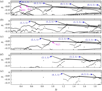
correspondingly. 35 eigenvalue/eigenvector pairs are converged at each position by the standard shift-and-invert Arnoldi algorithm. The resulting spectra are presented in figure 5. All eigenvalues are stable as expected. Two common features of the spectra are of special interest for the present study. First, the discrete mode branches indicated by their leading mode (blue), and second, a branch of continuous modes from which they emerge. The structure of the spectra is similar, but with a shift towards higher frequencies with increasing
 $m$
. The discrete branches are located approximately within the same frequency bands for all branches of even and odd
 $m$
, respectively. The least-damped mode marked as
 $(0,1,1)$
in figure 5(a) is found for
 $m=0$
and
 $St\approx 0.37$
. In what follows, the modal structures of the continuous and discrete modes are investigated in §§ 4.1 and 4.2, respectively.
Global stability spectra for (a)
 $m=0$
, (b)
 $m=1$
, (c)
 $m=2$
, (d)
 $m=3$
, (e)
 $m=4$
. The leading discrete modes (
 $\rightarrow$
(blue)) of each branch are indicated by the triplet
 $(m,n_{r},n_{x})$
, where
 $m$
is the azimuthal and
 $n_{r}$
and
 $n_{x}$
the radial and streamwise integer wavenumbers, respectively. This distinction of the discrete modes is addressed in the discussion of figure 8, below. Three continuous modes (
 $\rightarrow$
(pink)) shown in figure 6(b,d,e) are also indicated.

4.1 Features of the continuous branch
Figure 6 shows three representative side-by-side comparisons of coherent structures distilled from the LES via CSD (a,c,e) and global modes of the continuous branch (b,d,f). The eigenvalue corresponding to the mode shown in figure 6(b) is located right below the least-damped mode
 $(0,1,1)$
in figure 5, i.e. at
 $St\approx 0.37$
and
 $\unicode[STIX]{x1D714}_{i}\approx -0.04$
. This mode is mainly of K–H type with only a weak acoustic component inside the potential core. The modal shape compares well with the CSD from the LES data shown in figure 6(a). Here, the correlation location of the CSD is chosen such that it extracts the shear-layer instability component. A correlation location inside the potential core brings to light the trapped acoustic wave, as discussed later in the context of figure 7(a,b).
Comparison between (a,c,e) CSD of the LES with location
 $(x_{0},r_{0})$
marked by ‘
 $+$
’ and (b,d,f) global modes: (a,b)
 $m=0$
,
 $St\approx 0.37$
; (c,d)
 $m=0$
,
 $St\approx 0.5$
; (e,f)
 $m=2$
,
 $St\approx 1$
. Modes are compared in terms of their normalized pressure components (

 $-0.25\leqslant \text{Re}(\tilde{\tilde{p}}_{m,\unicode[STIX]{x1D714}})/\Vert \text{Re}(\tilde{\tilde{p}}_{m,\unicode[STIX]{x1D714}})\Vert _{\infty }\leqslant 0.25$
,
 $-0.25\leqslant \text{Re}(\hat{p}_{m})/\Vert \text{Re}(\hat{p}_{m})\Vert _{\infty }\leqslant 0.25$
).

A remarkable agreement is found for
 $m=0$
and
 $St=0.5$
as depicted in figure 6(c,d). Both the LES and the modal analyses identify a global structure that combines a K–H wave train with an acoustic core mode. The regions of support and the wavenumbers of both components are accurately predicted by the global mode. A similar modal structure can be seen in the
 $m=2$
,
 $St\approx 1$
case in figure 6(e,f). In this higher azimuthal wavenumber and frequency example, the CSD extracts the K–H wavepacket as the most energetic structure, whereas the trapped acoustic wave is dominant in the global mode.
In the spectrum, the continuous modes are unavoidably rendered discrete due to the numerical discretization. Changes in the numerical discretization scheme can freely shift their eigenvalues along the underlying continuous branch. Changing the computational domain size, as discussed in appendix C, is an example where such behaviour can be observed.
The physical aspect of interest for the present study is that the continuous modes consist of two coupled wave components: a downstream propagating K–H wavepacket, and a trapped acoustic wave in the potential core.
4.2 Features of the discrete modes
The leading discrete global modes of the first three branches for
 $m=0$
, and the first branch for
 $m=1$
are depicted in figures 7(b,d,f) and 7(h), respectively. Clearly, the discrete global modes represent the trapped acoustic mechanism. Unlike their continuous counterparts seen in figure 6(d,f) above, the discrete modes are confined within a small region
 $x\lesssim 2$
close to the nozzle. Their radial order
 $n_{r}$
becomes apparent by comparing modal shapes for different branches as in figure 7(b,d,f). For higher
 $m$
, the
 $n_{r}=1$
branch is shifted towards a higher frequency as can be deduced from figure 7(h) in comparison with the global spectra shown in figure 5. Note that all discrete global modes also possess a weaker K–H component, in contrast with the continuous modes which show K–H and trapped waves to be more strongly coupled. By comparison with the CSD (figure 7
a,c,e,g), it can be seen that the trapped acoustic modes are evidently present in the LES data. Their spatial extent and waveforms are accurately predicted by the linear global analysis. A similarly good agreement is found for all
 $m$
under consideration.
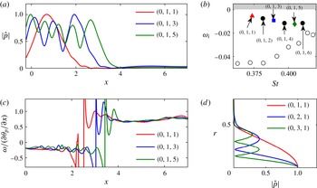
The pressure profile along the jet axis shown in figure 8(a) reveals the internal structure of the modes within a given branch. It can be seen that the absolute pressure signal possesses an increasing number of anti-nodes (now with respect to the
 $x$
axis) with increasing frequency. This suggests the definition of an integer streamwise wavenumber
 $n_{x}$
equal to the number of anti-nodes. Individual discrete modes can be identified by the triplet
 $(m,n_{r},n_{x})$
. The latter observation also has an important physical implication. The corresponding eigenvalues are reproduced in the detail of the spectrum in figure 8(b) for comparison. Figure 8(c) depicts the phase velocity of the same modes estimated as
 $\unicode[STIX]{x1D714}/(\unicode[STIX]{x2202}\unicode[STIX]{x1D703}_{p}/\unicode[STIX]{x2202}x)$
along the jet axis, where
 $\unicode[STIX]{x1D703}_{p}=\arg (\hat{p})$
is the local phase of the eigenvector pressure component. A jump discontinuity separates the pressure signal of each mode into part with a negative phase speed of
 $c_{p}\approx -0.2$
, and a part with a positive phase speed of
 $c_{p}\gtrsim 0.8U_{j}$
. The radial order
 $n_{r}$
previously addressed in the discussion of figure 7, is demonstrated in figure 8(d) in terms of radial velocity profiles of the leading modes of the first three branches for
 $m=0$
. In our parallel investigation, Towne et al. (Reference Towne, Cavalieri, Jordan, Colonius, Schmidt, Jaunet and Brès2017) show that these waves behave like acoustic waves that experience the potential core as a cylindrical duct with a pressure release surface. Accordingly, they are effectively trapped within the potential core and their radial structure takes the form of Bessel functions. Therefore, we refer to them as duct modes.
Comparison between (a,c,e,g) CSD of the LES with location
 $(x_{0},r_{0})$
marked by ‘
 $+$
(blue)’ and (b,d,f,h) global modes: (a,b)
 $m=0$
,
 $St\approx 0.37$
, mode
 $(0,1,1)$
; (c,d)
 $m=0$
,
 $St\approx 0.87$
, mode
 $(0,2,1)$
; (e,f)
 $m=1$
,
 $St\approx 0.6$
, mode
 $(1,1,1)$
. Modes are compared in terms of their normalized pressure components (

 $-0.25\leqslant \text{Re}(\tilde{\tilde{p}}_{m,\unicode[STIX]{x1D714}})/\Vert \text{Re}(\tilde{\tilde{p}}_{m,\unicode[STIX]{x1D714}})\Vert _{\infty }\leqslant 0.25$
,
 $-0.25\leqslant \text{Re}(\hat{p}_{m})/\Vert \text{Re}(\hat{p}_{m})\Vert _{\infty }\leqslant 0.25$
).

Characterization of trapped acoustic modes in the potential core for
 $m=0$
: (a) pressure magnitude along the jet axis; (b) detail of the spectrum showing the
 $(0,1)$
-branch (▴ (red), ▪ (blue) and ♦ (green), modes from (a,c); ● (black), other discrete modes; ○, continuous modes); (c) local phase velocity of the pressure along the jet axis; (d) pressure magnitude profiles at
 $x=1$
. All quantities are normalized with respect to their maximum value. The discrete modes are labelled as (
 $m$
,
 $n_{r}$
,
 $n_{x}$
), corresponding to their azimuthal wavenumber
 $m$
, their radial order
 $n_{r}$
obtained as shown in (d) and their streamwise order obtained as shown in (a), respectively.

5 Resonant acoustic modes
5.1 Comparison with LES
We next examine the structure of the discrete modes in more detail by comparing the modes of the
 $(0,1)$
branch with the simulation in terms of the estimated PSD defined by (2.9). In order to account for the small frequency spacing between individual modes, the spectral estimation is based on a larger number of 1024 snapshots in the following. This results in a smaller ensemble of
 $N_{b}=19$
realizations for the same overlap.
Comparison between the pressure components of LES power spectral density estimate (

 $0\leqslant \bar{P}_{pp}/\Vert \bar{P}_{pp}\Vert _{\infty }\leqslant 1$
) and global mode (
 $\hat{p}_{m}\hat{p}_{m}^{\ast }$
, —— (blue)) for branch
 $(0,1)$
: (a)
 $St\approx 0.374$
, mode
 $(0,1,1)$
; (b)
 $St\approx 0.382$
, mode
 $(0,1,2)$
; (c)
 $St\approx 0.39$
, mode
 $(0,1,3)$
; (d)
 $St\approx 0.397$
, mode
 $(0,1,4)$
; (e)
 $St\approx 0.405$
, mode
 $(0,1,5)$
; (f)
 $St\approx 0.41$
, mode
 $(0,1,6)$
. Contours of
 $\hat{p}_{m}\hat{p}_{m}^{\ast }$
correspond to 20 %, 40 %, 60 % and 80 % of its maximum value.

Figure 9 shows that we find a very good agreement between the global modes and the LES in terms of the location and structure of the trapped acoustic waves. The number of maximum nodes agrees precisely with our definition of the streamwise wavenumber
 $n_{x}$
, as introduced in the context of figure 8(a). The trapped acoustic waves are spatially confined in the streamwise direction. In the inlet plane, we find that the nozzle impedance associated with the LES simulation is well mimicked by the inlet sponge boundary condition. This favourable agreement was found robust with respect to changes in the sponge layer intensity, as detailed in appendix B. The length of the region over which the trapped waves have support is frequency dependent. For example, mode
 $(0,1,1)$
in figure 9(a) has a streamwise spatial support of
 $0\lesssim x\lesssim 2$
, whereas mode
 $(0,1,6)$
shown in figure 9(a) is confined within
 $0\lesssim x\lesssim 3.5$
. The observation is explained by the existence of a frequency-dependent end condition related to the streamwise contraction of the potential core. We identify this end condition using weakly non-parallel stability theory in Towne et al. (Reference Towne, Cavalieri, Jordan, Colonius, Schmidt, Jaunet and Brès2017), and compare the prediction to the spatial support of the global modes in § 5.6.
5.2 Experimental observations
Figure 10 compares discrete mode frequencies to spectra obtained from two sets of experimental data. In a recent experimental campaign dedicated to the validation of the present LES, the near-field pressure of a
 $M=0.9$
turbulent jet was measured in the ‘Bruit and Vent’ jet noise facility of the Pprime Institute, Poitiers. In a similar experiment by Suzuki & Colonius (Reference Suzuki and Colonius2006, appendix B) for
 $M_{j}=0.98$
,
 $T_{j}/T_{\infty }=0.84$
and
 $\text{Re}=16\times 10^{5}$
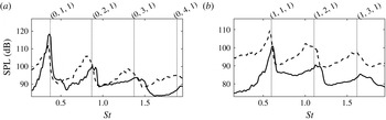
, the measured tones were attributed to an acoustic duct phenomenon upstream of the nozzle. Both experiments used a six microphone ring array located in the near-nozzle region. Spectra for the axisymmetric and first helical Fourier components are reproduced in panels 10(a) and 10(b), respectively. It can be seen that the peaks in the spectra agree well with the frequencies of the leading discrete modes found by the global analysis.
Near-nozzle exit spectrum comparing Strouhal numbers of the least-damped global modes (
 $\cdots \cdots$
) to the sound pressure level (SPL) of recent ‘Bruit and Vent’ measurements (——), and the data of Suzuki & Colonius (Reference Suzuki and Colonius2006) (– – –) for
 $M_{j}=0.98$
,
 $T_{j}/T_{\infty }=0.84$
: (a)
 $m=0$
; (b)
 $m=1$
.

5.3 Frequency–wavenumber analysis
Our next goal is to describe the trapped acoustic instabilities in the frequency–wavenumber domain. For a fixed frequency
 $\unicode[STIX]{x1D714}$
and azimuthal wavenumber
 $m$
, the streamwise wavenumber content of the trapped modes can readily be obtained from a Fourier decomposition of pressure signal on or parallel to the jet axis. Here, we chose
 $\tilde{\tilde{p}}_{m,\unicode[STIX]{x1D714}}(0\leqslant x\leqslant 5,r_{0})$
, and denote by
 $k$
the streamwise wavenumber. The exact length and radial location of the line segment used for the decomposition has no significant effect on the results, as long as it remains located inside the potential core. Windowing or padding of the segment is not necessary for the same reasons.
Frequency–wavenumber diagram (

 $\bar{P}_{pp}(0\leqslant x\leqslant 5,r_{0})$
) of the LES data in the potential core region for
 $m=0$
and
 $r_{0}=0.1$
. Lines of constant propagation velocity
 $c_{p}=\unicode[STIX]{x1D714}/k=c_{g}=\unicode[STIX]{x2202}\unicode[STIX]{x1D714}/\unicode[STIX]{x2202}k$
and their corresponding values are shown in colour.
 $c_{p}=0.8U_{j}$
corresponds to the propagation speed of K–H instabilities.

The resulting frequency–wavenumber diagram for
 $m=0$
is shown in figure 11. The PSD is estimated by means of equation (2.9). In the positive
 $k$
-plane, energy is concentrated along the line of constant slope
 $\unicode[STIX]{x1D714}/k\approx 0.8U_{j}$
(—— (pink)), corresponding to the typical downstream propagation velocity of the initial jet shear-layer instability. The curved bands of energy in the angular sector of negative phase velocities
 $-a_{j}\leqslant c_{p}\leqslant U_{j}-a_{j}$
are the signatures of the trapped acoustic modes. These bands can be interpreted as empirical dispersion relations of the K–H and trapped acoustic modes, as they relate their frequency to their wavenumber. The lowest band originates from trapped acoustic modes of radial order
 $n_{r}=1$
, the second of
 $n_{r}=2$
and so forth. Note that the shape of the energy bands implies that multiple waves with negative phase velocity can coexist at certain frequencies. Furthermore, it can be observed that the two ends of each band asymptotically approach the lines
 $U_{j}-a_{j}$
and
 $-a_{j}$
, respectively. These two limits correspond to acoustic duct behaviour (– – – (green)) with waves propagating against the jet velocity inside the potential core and acoustic free-stream behaviour (– – – (blue)), with waves propagating upstream in the ambient flow.
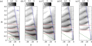
LES power spectral density in form of a frequency–wavenumber diagram obtained from the pressure signal along the jet axis in the potential core
 $x\in [0\;5]$
: (a)
 $m=0$
; (b)
 $m=1$
; (c)
 $m=2$
; (d)
 $m=3$
; (e)
 $m=4$
. The Strouhal numbers of the leading global modes of each discrete branch (
 $\cdots \cdots$
(red); marked by ‘
 $\rightarrow$
(blue)’ in figure 5) are shown for comparison.

Details focusing on the trapped acoustic instability mechanism for higher azimuthal wavenumbers are presented in figure 12. It can be seen that the onset of the acoustic instability is shifted towards higher frequencies with increasing azimuthal wavenumber
 $m$
. A comparison with the global stability spectra shown in figure 5 confirms that the the local minima (valleys) occur precisely at the frequencies of the leading global modes of each discrete branch. For
 $m=0$
and
 $m=1$
, the PSD peaks within the
 $n_{r}=1$
energy bands, whereas higher radial order modes are most energetic for
 $m>1$
.
5.4 Reconstruction of the dispersion relation from global modes
We now focus on the wavenumber content of the global modes for a direct comparison with the LES. A frequency–wavenumber diagram analogous to figure 11 can be constructed from the global modes using exactly the same method as described above. For each mode, a Fourier decomposition of the pressure
 $\hat{p}_{m}(0\leqslant x\leqslant 5,r_{0})$
yields a wavenumber spectrum as depicted in figure 13(c). In the particular case of mode
 $(0,1,2)$
in this example, the spectrum exhibits three distinct peaks denoted by ‘
 $k^{-}$
’, ‘
 $k^{+}$
’ and ‘K–H’.
Reconstruction of the dispersion relations of the trapped acoustic and K–H instabilities from a spectral analysis of the pressure signal along the jet axis in the potential core
 $x\in [0\;5]$
: (a) frequency–wavenumber diagram comparing LES (

 $\bar{P}_{pp}$
) as in figure 12(a), and global modes (● (red), mode
 $(0,1,1)$
; —— (red), – – – (red), trapped-mode branches; – – – (green), – – – (blue), continuous modes; —— (pink), K–H component); (b) LST spectrum around branch
 $(0,1)$
(● (red), mode
 $(0,1,1)$
;
 $+$
(red)branch intersection mode; ○ (red) other
 $(0,1)$
modes; ▿ (blue), ▫ (green) continuous modes); (c) wavenumber spectrum of mode
 $(0,1,2)$
. Colours and symbols in (a) and (b) correspond. Since all modes comprise a K–H component, it is not indicated in (b).

The ‘
 $k^{-}$
’, ‘
 $k^{+}$
’ and ‘K–H’ peaks are identified for all discrete modes. Connecting them in the
 $St$
–
 $k$
plane yields the red lines in figure 13(a). Analogously, the leading (– – – (blue), free-stream behaviour) and trailing (– – – (green), duct behaviour) sections are found by connecting the dominant peaks in the spectrum of the continuous modes in negative
 $k$
-plane. Continuous segments can now readily be interpreted as reconstructed dispersion relations for the trapped waves and the K–H waves.
A detail of the spectrum around branch
 $(0,1)$
is reproduced in figure 13(b) using the same colours and symbols as in the frequency–wavenumber diagram in figure 13(a) for comparison. The concave part (red) of the lower band is directly associated with the discrete branch
 $(0,1)$
modes. Analogously, the upper band at
 $St\gtrsim 0.8$
is associated with the
 $(0,2)$
branch.
The mode located at the discrete-continuous branch intersection (
 $+$
(red)) in figure 13(a,b) separates continuous from discrete, and also continuous duct modes from continuous free-stream modes. The local slope along each segment of the dispersion relation determines the group velocity of the instability wave at the corresponding wavenumber and frequency. This motivates the distinction between a
 $k^{+}$
(—— (red)) segment of positive, and a
 $k^{-}$
(– – – (red)) segment of negative group velocity, respectively. A remarkable agreement between the reconstructed and the empirical dispersion relations is found. The discrete global modes contain both the
 $k^{+}$
and the
 $k^{-}$
wave. This observation shows that these two waves are intimately linked, and suggests a resonance phenomenon, as we will confirm in the following.
Of particular interest are the two end points of the
 $k^{+}$
segment as they mark zeros of the slope of the dispersion relation, and therefore points of zero group velocity. These points are of particular interest as they determine the long-time behaviour of a system in a fixed laboratory reference frame (Briggs Reference Briggs1964). The lower point, denoted as S1, is associated with the leading mode and the upper one, denoted by S2, with the mode that marks the intersection of the discrete branch with the continuous spectrum. These points describe the transition from a mechanism that is predominantly active close to or inside the shear layer, i.e. continuous free-stream modes, to a duct-like behaviour inside the core, i.e. to continuous core modes. The anti-nodes used to determine the integer streamwise wavenumber
 $n_{x}$
, and as seen in figures 8(a) and 9, can now be interpreted in the light of the above discussion as a beating
 $$\begin{eqnarray}\text{e}^{\text{i}k^{+}x}+\text{e}^{\text{i}k^{-}x}=2\cos \left(\frac{\unicode[STIX]{x0394}k^{\pm }}{2}x\right)\exp \left(\text{i}\frac{k^{+}+k^{-}}{2}x\right)\end{eqnarray}$$
resulting from the superposition of the
 $k^{+}$
and the
 $k^{-}$
waves. As an example, consider mode
 $(0,1,3)$
with
 $k^{+}=-7.1$
,
 $k^{-}=-13.0$
and a resulting difference of
 $\unicode[STIX]{x0394}k^{\pm }=5.9$
. The corresponding wavelength of the beating,
 $\unicode[STIX]{x1D706}^{\pm }=4\unicode[STIX]{x03C0}/\unicode[STIX]{x0394}k^{\pm }=2.1$
, can be seen to accurately match twice the distance of the maximum nodes of mode
 $(0,1,3)$
in figure 8(a). The average wavenumber
 $(k^{+}+k^{-})/2$
on the other hand determines the wavelength seen in instantaneous, or visualizations of the real part as in figure 7. Together with the observation that the acoustic modes are confined within a short region in the streamwise direction by end conditions, it can be concluded at this point that a resonance between the
 $k^{+}$
and
 $k^{-}$
segments occurs. The resonance phenomenon in turn explains the high energy content along the frequency band in which
 $k^{+}$
and
 $k^{-}$
coexist. For the same reason, the corresponding modes appear as discrete eigenvalues in the spectrum.
For frequencies below the lowest radial order discrete branch, e.g.
 $St\lesssim 0.37$
for
 $m=0$
, the potential core does not support duct modes. The absence of the duct mechanism appears to be directly related to the sudden drop of the eigenvalues at low
 $St$
in the global stability spectra, as seen in figure 5 above. This becomes particularly apparent at higher azimuthal wavenumbers. For
 $m=3$
in figure 5(d), for example, all modes are heavily damped up to
 $St\approx 1$
. As soon as duct modes are supported, the discrete mode branch
 $(3,1)$
appears above a branch of K–H modes which now support acoustic core waves.
A caveat on the comparison between the reconstructed and the empirical dispersion relations is that the discrete nature of the trapped acoustic modes is not evident from the LES data. In the LES frequency–wavenumber diagram, the energy appears to be smoothly distributed along the individual bands. Presumably, a much longer time series would be needed to converge the statistics of individual discrete modes.
5.5 Isolation of the trapped acoustic waves
In classical local stability theory, each spatial mode is associated with a complex wavenumber given by its eigenvalue. By contrast, a single global mode of a specific complex frequency can encapsulate a variety of waves. We are interested in isolating the trapped acoustic wave component from the global modes to determine their spatial support, and for comparison with local theory.
Same as figure 9 but comparing LES power spectral density estimate (

 $0\leqslant \bar{P}_{pp}/\Vert \bar{P}_{pp}\Vert _{\infty }\leqslant 1$
) and the isolated trapped acoustic modes (
 $\Vert \hat{q}_{m}(x_{0},r_{0})\Vert \cdot \Vert \hat{q}_{m}^{\dagger }(x_{0},r_{0})\Vert$
, —— (blue)). Contours of the product map correspond to 20 %, 40 %, 60 % and 80 % of its maximum value.

We have observed that adjoint trapped modes have a negligible K–H component. Examples and a brief discussion of the adjoint modes used here can be found in appendix E. Hence, the map of the local product
 $$\begin{eqnarray}\Vert \hat{q}_{m}(x_{0},r_{0})\Vert \cdot \Vert \hat{q}_{m}^{\dagger }(x_{0},r_{0})\Vert\end{eqnarray}$$
is a way of isolating the trapped-wave mechanism from the K–H wavepackets. In a different context, such maps have been used by Chomaz (Reference Chomaz2005) and Giannetti & Luchini (Reference Giannetti and Luchini2007) to determine an upper bound for the sensitivity of eigenvalues to spatially localized feedback. Figure 14 compares the map of the direct-adjoint product with the estimated PSD from the simulation.
The analysis clearly identifies the maximum nodes of the pressure PSD as the regions of highest sensitivity, and therefore closely resembles the PSD distribution of the global modes as seen in figure 9. Comparing figures 9 and 14, it becomes evident that multiplying the direct solution by the adjoint largely removes the shear-layer wavepackets. We can thus make use of the direct-adjoint product as a filter. The K–H instability constitutes a convective non-normality characterized by an upstream–downstream separation of the spatial support of the adjoint and direct modes (Sipp et al. Reference Sipp, Marquet, Meliga and Barbagallo2010; Nichols & Lele Reference Nichols and Lele2011). It is therefore widely eliminated from the product and the trapped waves are clearly isolated. Furthermore, the match between the PSD and the isolated trapped modes suggests that the trapped instability mechanism is nearly self-adjoint.
5.6 Local linear theory
The study of the resonant trapped acoustic modes in terms of local and weakly non-parallel spatio-temporal linear theory is at the core of the parallel investigation by Towne et al. (Reference Towne, Cavalieri, Jordan, Colonius, Schmidt, Jaunet and Brès2017). Here, we revisit one of the main findings of the weakly non-parallel theory regarding the end condition of the resonant modes, as it allows for a direct comparison with the global modes. In particular, we are interested in finding saddle points in the complex
 $k$
-plane, i.e. the points
 $k_{0}$
at which
 $\unicode[STIX]{x2202}\unicode[STIX]{x1D714}/\unicode[STIX]{x2202}k=0$
. In such saddle points,
 $k_{0}$
is a double root of the dispersion relationship. These points are relevant to provide end conditions if they are formed between a
 $k^{+}$
and a
 $k^{-}$
mode (Huerre & Monkewitz Reference Huerre and Monkewitz1990). Defining
 $\unicode[STIX]{x1D714}_{0}=\unicode[STIX]{x1D714}(k_{0})$
(i.e.
 $\unicode[STIX]{x1D714}_{0}$
and
 $k_{0}$
satisfy the locally parallel dispersion relationship), if
 $\unicode[STIX]{x1D714}_{0}$
is real, a saddle point presumably corresponds to the points S1 and S2 in the reconstructed dispersion relation shown in figure 13. The reader is referred to Towne et al. (Reference Towne, Cavalieri, Jordan, Colonius, Schmidt, Jaunet and Brès2017) for a detailed discussion. Under the assumption of a locally parallel flow, i.e. homogeneity in the streamwise direction, the normal-mode ansatz (2.2) takes the form
 $$\begin{eqnarray}q^{\prime }(r,\unicode[STIX]{x1D703},t)=\hat{q}_{m}(r)\text{e}^{\text{i}(kx+m\unicode[STIX]{x1D703}-\unicode[STIX]{x1D714}t)},\end{eqnarray}$$
where the streamwise wavenumber
 $k\in \mathbb{C}$
is a free parameter. The resulting eigenvalue problem for
 $\unicode[STIX]{x1D714}$
at some streamwise location
 $x_{0}$
takes the same form as in 2.3, but with
 ${\mathcal{L}}_{m}={\mathcal{L}}_{m}(\bar{q}(x_{0},r),k)$
now as the local linear stability operator. Saddle points are identified in the complex
 $k$
-plane by solving the local eigenvalue problem over a range of complex wavenumbers
 $k$
and subsequently finding the zeros of the complex derivative of
 $\unicode[STIX]{x1D714}(k)$
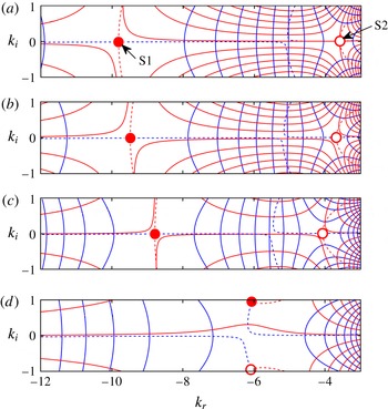
for a specific mode. In figure 15, the acoustic core modes of radial order
 $n_{r}=1$
are traced in the complex plane. Two saddles S1 and S2 are found for
 $x$
locations close to the nozzle. Both saddles reside on the real axis, and move closer together with increasing downstream distance, as seen in figure 15(a–c). At a certain streamwise location, the two saddles collide. For locations further downstream, no saddle points with real valued
 $k_{0}$
are found. Beyond this point, no
 $k^{+}$
-mechanism exists, and resonance cannot occur. This case is depicted in figure 15(d).
Saddle point location of the
 $(0,1)$
branch in the complex wavenumber plane obtained from local spatio-temporal stability theory at different streamwise positions: (a)
 $x=0$
; (b)
 $x=1.5$
; (c)
 $x=2.5$
; (d)
 $x=3.8$
. Isolines of the real and imaginary part of the complex frequency (—— (blue),
 $\unicode[STIX]{x1D714}_{r}$
; —— (red),
 $\unicode[STIX]{x1D714}_{i}$
) are shown, and the locations of the two saddle points (● (red), saddle S1; ○ (red), saddle S2) are obtained as the zeros of the complex derivative
 $\text{Re}(\unicode[STIX]{x2202}\unicode[STIX]{x1D714}/\unicode[STIX]{x2202}ks)=\text{Im}(\unicode[STIX]{x2202}\unicode[STIX]{x1D714}/\unicode[STIX]{x2202}ks)=0$
(– – – (blue),
 $\text{Re}(\unicode[STIX]{x2202}\unicode[STIX]{x1D714}/\unicode[STIX]{x2202}k)$
; – – – (red),
 $\text{Im}(\unicode[STIX]{x2202}\unicode[STIX]{x1D714}/\unicode[STIX]{x2202}k)$
. Note that in (d), the saddles S1 and S1 cannot be distinguished, and the assignment is therefore arbitrary.

Comparison between local spatio-temporal stability theory (—— (red), first saddle point location; – – – (red), second saddle point location), isolated trapped modes (blue areas), and mode at the branch intersection (green areas), denoted by ‘
 $+$
(red)’ in figure 13(a,b) for branch
 $(0,1)$
). The normalized direct-adjoint product is shown along the jet axis for
 $m=0$
, and along
 $r_{0}=0.25$
for
 $m=1$
in (b). The trapped modes clearly confined between the inlet and the saddle point locations.

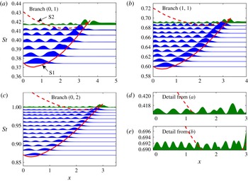
In figure 16, the frequency of the two saddle points is plotted over the streamwise location (—— (red), – – – (red)) for three representative branches. The
 $(0,1)$
branch is considered in figure 16(a) and higher azimuthal wavenumber and radial order examples in panels 16(b) and 16(c), respectively. The isolated resonant acoustic modes (▪ (blue)) and the branch intersection mode (▪ (green)) are shown in the same plots for comparison. A good agreement between the spatial support of the resonant waves, as identified by the global stability analysis and the location of the S1 saddle, is found in all cases. It becomes apparent that the saddle point serves as an end condition for the trapped acoustic modes. With increasing
 $St$
, resonance first occurs for the leading discrete mode of axial order
 $n_{x}=1$
at the lowest possible frequency that permits the interaction between two waves of opposite group velocity with
 $k^{+}\approx k^{-}$
. At higher frequencies, the beating between the two waves
 $k+>k^{-}$
causes the observed modulation of the trapped modes of streamwise order
 $n_{x}>1$
. The frequency of the highest streamwise wavenumber mode approximately coincides with the minimum frequency of the S2 saddle. Beyond this point, no resonant core modes are to be found. Apparently, the S2 saddle provides an alternative end condition. In contrast to the S1 saddle, S2 is associated with a
 $k^{-}$
wave which apparently has a lower reflection coefficient at the nozzle than the duct modes. This becomes apparent from an inspection of the branch intersection modes (▪ (green)). The signature of the S1 saddle is clearly visible, but the fluctuation levels between the nozzle and S1 are much lower than for the discrete modes. From the detail views depicted in panels 16(d) and 16(e), respectively, the influence of the S2 saddle can be inferred in the case of the
 $(0,1)$
and
 $(1,1)$
branches, respectively. A clear beating signature is visible only between the nozzle exit and S2, whereas the fluctuation has a richer wavenumber content between S1 and S2.
The side-by-side comparison of local and global stability results in figure 16 highlights the complementary merits of both approaches. The global mode analysis reveals the connection between the different stability phenomena, identifies internal feedback and predicts the acoustic resonance. On the other hand, the local approach provides further physical insight about the physical identity of the waves and the nature of the end conditions.
6 Summary and conclusions
Linear global stability modes are found to well represent large-scale coherent structures in a natural turbulent
 $M_{j}=0.9$
jet. Coherent structures were extracted from the LES database by means of spectral estimation techniques, and directly compared to the global modes. The favourable agreement extended over a range of frequencies and for azimuthal wavenumbers
 $0\leqslant m\leqslant 4$
.
Apart from the well-known K–H wavepackets in the shear layer, trapped acoustic waves that are confined within the potential core are observed. In the global stability spectrum, these trapped acoustic waves appear in two forms. They are either part of the continuous branch, or appear in branches of lightly damped discrete modes. The continuous acoustic waveforms can be further distinguished into two categories. Continuous duct modes are strictly confined within the potential core and propagate upstream with
 $c_{p}\gtrsim U_{j}-a_{j}$
, whereas continuous free-stream modes propagate with a phase velocity of
 $c_{p}\lesssim -a_{j}$
. This associates them with the ambient flow outside of the shear layer.
Branches of discrete acoustic modes appear in the spectrum in a hierarchical order determined by their radial wavenumber. They possess two wave components, both of negative phase velocity, but of group velocities of opposite sign denoted as
 $k^{+}$
and
 $k^{-}$
waves, respectively. The contraction of the potential core with downstream distance imposes a frequency-dependent end condition on the trapped acoustic waves. The nozzle impedance in the inlet plane provides the second end condition. At certain frequencies, the distance from the nozzle to the downstream end condition becomes an integer multiple of the wavenumber difference of the two waves, and an acoustic resonance in the form a beating occurs. The dispersion relation of the trapped acoustic modes was reconstructed from the global modes, and found in remarkable agreement with an empirical frequency–wavenumber diagram extracted from the LES.
In Towne et al. (Reference Towne, Cavalieri, Jordan, Colonius, Schmidt, Jaunet and Brès2017), we suggest that the upstream and downstream end conditions for the resonance are provided by turning points originating from the nozzle impedance and the streamwise contraction of the potential core, respectively. The interpretation that the saddles in the complex
 $k$
-plane act as turning points for the trapped waves is confirmed by the favourable agreement between the saddle point locations and the spatial support of the global modes. A simplified cylindrical vortex sheet model also allows us to study the Mach number dependency of the trapped acoustic mechanism. The model predicts two neutral saddle points, and therefore resonance, in the narrow range of Mach numbers
 $0.82<M_{j}<1$
for isothermal jets. For Mach numbers outside of this range, the model predictions are consistent with the findings of Tam & Hu (Reference Tam and Hu1989).
The present study shows that intrinsic stability mechanisms, such as the resonant trapped acoustic modes, are brought to light by laminar global linear stability analysis of the turbulent mean flow. They appear as distinct eigenvalues in the spectrum, and the corresponding eigenvectors accurately represent the average coherent structures educed from the data. The underlying assumption of the approach is hence justified a posteriori.
Further details may be found in the appendices. Appendix A motivates the choice of parameters for the global stability study, and gives details on the numerical discretization and the damping region. The appendices B, C, D and E address the influence of the inlet sponge layer on the trapped acoustic modes, the effect of domain truncation, the effect of the Reynolds number, and the adjoint solutions to the trapped acoustic modes, respectively. In appendices B–D, the spectrum of the production run set-up with a solution domain of size
 $x,r\in [0,25]\times [0,2.25]$
, a Reynolds number of
 $Re=10^{5}$
, and sponge intensity of
 $\unicode[STIX]{x1D716}_{sponge}=5$
is reproduced as a reference.
Acknowledgements
O.T.S. gratefully acknowledges support by DFG grant no. 3114/1-1. We gratefully acknowledge support from the Office of Naval Research under contract N0014-11-1-0753 and N00014-16-1-2445. A.V.G.C. and P.J. acknowledge support from the Science Without Borders program (project number A073/2013). We are grateful to S. Piantanida and R. Kari for conducting the ‘Bruit and Vent’ measurements. The LES study was supported by NAVAIR SBIR project, under the supervision of Dr J. T. Spyropoulos. The main LES calculations were carried out on CRAY XE6 machines at DoD HPC facilities in ERDC DSRC.
Appendix A. Computational set-up
The computational domain
 $\unicode[STIX]{x1D6FA}$
outlined in figure 1(a) is discretized by a
 $1150\times 250$
points Cartesian grid. The solution domain
 $x,r\in [0,25]\times [0,2.25]$
is padded by a sponge region to prevent reflections from the boundaries. The resulting overall domain size is
 $x,r\in [-1.2,26.2]\times [0,2.8]$
. A parallel flow corresponding to the inlet profile
 $\bar{q}(0,r)$
is assumed in the inlet sponge layer region
 $x<0$
. The domain is constructed by first defining an equidistantly spaced mesh over
 $x,r\in [-0.5,25.5]\times [0,2.5]$
, and second applying an exponential grid stretching of the form
 $\exp (1.5\unicode[STIX]{x1D702})$
to the region outside of the solution domain.
 $0\leqslant \unicode[STIX]{x1D702}\leqslant 1$
is the normalized coordinate normal to the respective boundary, or the local sponge layer coordinate. Inside this region, the base state is assumed to be parallel, and the solution is penalized by a forcing of the form
 $-\unicode[STIX]{x1D716}_{sponge}(6\unicode[STIX]{x1D702}^{5}-15\unicode[STIX]{x1D702}^{4}+10\unicode[STIX]{x1D702}^{3})$
, where
 $\unicode[STIX]{x1D702}$
is now normalized with respect to the stretched coordinate. A fifth-order polynomial distribution smoothly ramps the source term from zero to
 $\unicode[STIX]{x1D716}_{sponge}=5$
. The support of the trapped acoustic modes that are the main subject of the linear stability study is limited to the potential core in the downstream and radial directions. The sponge has therefore a negligible influence on these modes in these directions. In absence of the nozzle in the computational domain, the inlet sponge layer plays an important role in mimicking the inlet impedance experienced by upstream-travelling waves in the core, as further addressed in appendix B.
The spatial resolution used was found sufficient to resolve the increasingly fine modal structures up to
 $St\approx 2$
. In the radial direction, the resolution is chosen such that the jet boundary layer in the inlet plane, and therefore the initial shear layer, is resolved by
 $\unicode[STIX]{x1D6FF}_{inlet}/\unicode[STIX]{x0394}r=0.08/0.010=8$
grid points. Under the assumption that the dominant shear-layer instability advects at a phase speed of
 $c_{ph}\approx 0.8U_{j}$
(see § 4.2), a resolution of
 $\unicode[STIX]{x1D706}_{K{-}H}/\unicode[STIX]{x0394}x=0.39/0.023\approx 17$
grid points per wavelength is achieved at
 $St=2$
, the maximum Strouhal number considered.
Appendix B. Inlet sponge layer influence
The nozzle exit plane plays a crucial role as an end condition for the resonating trapped modes, as discussed in § 5. If is therefore important that the inlet sponge layer region correctly accounts for the unknown nozzle impedance.
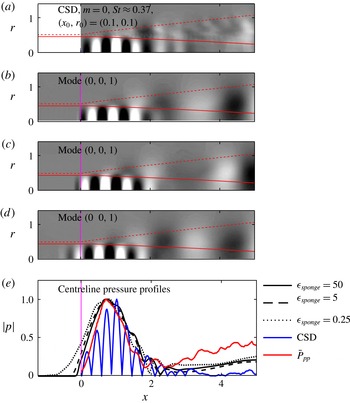
Influence of the sponge gain
 $\unicode[STIX]{x1D716}_{sponge}$
on trapped acoustic modes and comparison with LES: (a) CSD of the LES as in figure 7(a); global modes with (b)
 $\unicode[STIX]{x1D716}_{sponge}=50$
, (c)
 $\unicode[STIX]{x1D716}_{sponge}=5$
, and (d)
 $\unicode[STIX]{x1D716}_{sponge}=0.25$
; (e) centreline pressure profiles. The same contour levels as in figure 7 are used in (a–d), and all profiles are normalized to unit maximum amplitude in (e). The LES PSD (
 $\bar{P}_{pp}$
, —— (red)) in (e) corresponds to the PSD along the axis in figure 9(a). The vertical magenta line indicates the beginning of the inlet sponge region in
 $x<0$
.

Figure 17 compares global mode pressure fields and pressure profiles along the centreline to the LES data. The least damped global mode
 $(0,0,1)$
is chosen as an example. It can be seen that the global mode pressure fields in figure 17(b–d) are in good agreement with the LES CSD in figure 17(a) despite the wide range of sponge intensities
 $0.25\leqslant \unicode[STIX]{x1D716}_{sponge}\leqslant 50$
. The centreline profiles reproduced in figure 17(e) allow for a more quantitative comparison. The LES PSD pressure peak location and profile shape of the trapped disturbance is accurately predicted by the global analysis for the two higher sponge gain cases. The comparison is less favourable for the
 $\unicode[STIX]{x1D716}_{sponge}=0.25$
. The low gain in this case allows the trapped wave to penetrate into the sponge layer, and the pressure peak gets shifted towards the inlet. An intermediate value of
 $\unicode[STIX]{x1D716}_{sponge}=5$
was found adequate to prevent reflections from any of the boundaries, and to mimic the inlet impedance at the same time. The favourable agreement between the modal structures predicted by the linear analysis and those extracted from the LES seen in figures 7, 9 and 14 confirms this statement.
Appendix C. Domain size influence
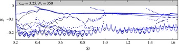
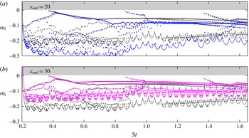
We first study the effect of the radial domain extent by comparing the reference spectrum to one obtained using a 44 % higher computational domain in figure 18. In the following, the lengths
 $r_{end}$
and
 $x_{end}$
denote the domain length excluding the sponge region in the radial and streamwise directions, respectively. The number of grid points is increased accordingly to keep the radial grid spacing comparable. The two spectra coincide to a large degree for all but the lowest frequencies
 $St\lesssim 0.35$
. At these low frequencies, an inspection of the eigenvectors shows that they get truncated in the radial direction towards the end of the domain. For the Strouhal number regime of interest, and in particular for the trapped acoustic modes, the radial domain size of the reference grid is found sufficient.
Influence of the far-field boundary location on the global spectrum: the reference solution with
 $r_{end}=2.25$
(● (grey), reference) is compared to an enlarged domain (● (blue), higher domain) with
 $r_{end}=3.25$
. The number of grid points in the radial direction is increased to
 $N_{r}=350$
for the higher domain. The computed area of each spectrum is outlined in the respective colour.

Influence of the domain length on the global spectrum: the reference solution with
 $x_{end}=25$
(● (grey), reference) is compared to a shortened domain with
 $x_{end}=20$
(● (blue), shorter domain) in (a), and an elongated domain with
 $x_{end}=30$
(● (pink), longer domain) in (b). The computed area of each spectrum is outlined in the respective colour.

The effect of domain truncation in the streamwise direction is more critical for convection dominated flows and was addressed in detail by Nichols & Lele (Reference Nichols and Lele2011) and Garnaud et al. (Reference Garnaud, Lesshafft, Schmid and Huerre2013a ). The latter authors found that the heads of the branches that correspond to upstream-propagating subsonic modes described by the local theory of Tam & Hu (Reference Tam and Hu1989) remained fixed within the spectrum for their enlarged domain while the continuous K–H mode branches get significantly shifted. Similarly, the continuous mode branches in our calculations get shifted downwards and upwards when the domain length is decreased as can be seen in panels 19(a) and 19(b), respectively. Below a certain frequency, this behaviour is not observed. In any case, the eigenvalues of the trapped acoustic modes that are the main focus of this paper are not influenced by the axial domain truncation. This observation is in accordance what Nichols & Lele (Reference Nichols and Lele2011) observed for the closely related upstream-propagating subsonic modes in their supersonic laminar jet.
Appendix D. Reynolds number effects
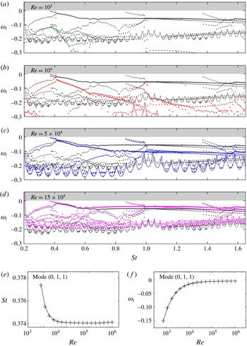
Influence of the Reynolds number on the global spectrum: (a) ● (green),
 $Re=10^{3}$
; (b) ● (red),
 $Re=10^{4}$
; (c) ● (blue),
 $Re=5\times 10^{4}$
; (d) ● (pink),
 $Re=15\times 10^{4}$
; (e) Strouhal number and (f) amplification rate dependence of mode
 $(0,1,1)$
. The reference solution with
 $Re=10^{5}$
(● (grey), reference) is reproduced in (a–d) for comparison. The computed area of each spectrum is outlined in the respective colour in (a–d).

A crucial parameter for this study is the Reynolds number, and since we investigate the stability of a turbulent mean flow, the choice is not obvious. The turbulent mean flow is a solution to the Reynolds-averaged Navier–Stokes (RANS) equations with an appropriate turbulence model. The RANS equations can be linearized about the mean flow, as demonstrated by Crouch, Garbaruk & Magidov (Reference Crouch, Garbaruk and Magidov2007) and Meliga, Pujals & Serre (Reference Meliga, Pujals and Serre2012). The results, however, are not necessarily superior to those obtained by using the linearized Navier–Stokes equations based on the molecular viscosity, as shown by Mettot, Sipp & Bézard (Reference Mettot, Sipp and Bézard2014). Garnaud et al. (Reference Garnaud, Lesshafft, Schmid and Huerre2013b
), for example, chose a molecular viscosity corresponding to
 $Re=1000$
for their study of a turbulent jet mean flow model, noting that the choice is rather arbitrary. Other authors like Jeun et al. (Reference Jeun, Nichols and Jovanović2016) considered the inviscid limit by linearizing the Euler equations.
Comparison of direct (a,c,e,g) and adjoint (b,d,f,h) global modes: (a,b) least damped mode
 $(0,1,1)$
; (c,d) higher streamwise order mode
 $(0,1,3)$
; (e,f) higher radial order mode
 $(0,2,1)$
; (g,h) higher azimuthal wavenumber mode
 $(1,1,1)$
. The normalized pressure (

 $-0.1\leqslant \text{Re}(\hat{p}_{m})/\Vert \text{Re}(\hat{p}_{m})\Vert _{\infty }\leqslant 0.1$
) is shown.

To address the Reynolds number effect, we compute spectra for different Reynolds numbers spanning two orders of magnitude, and compare them in figure 20(a–d). At the lowest Reynolds number
 $Re=10^{3}$
in figure 20(a), the spectrum appears more damped and the trapped acoustic modes are not observed. This is an imported result as it indicates that crucial physical aspects can be missed when the Reynolds number is chosen too small. When the Reynolds number is increased to
 $Re=10^{4}$
in figure 20(b), the trapped modes clearly appear in the spectrum. Increasing the Reynolds number further reveals that the first trapped acoustic mode branch becomes effectively Reynolds number independent for
 $Re\gtrsim 5\times 10^{4}$
. This is also observed for the higher radial mode branches, but at higher Reynolds numbers. The convergence of the frequency and amplification rate of the leading mode
 $(0,1,1)$
is further detailed in panels 20(e) and 20(f), respectively. Notably, the Strouhal number changes only in the third significant digit over the three orders of magnitude considered. The continuous mode branches, however, get shifted up with increasing Reynolds number. This result is in accordance with the findings by Garnaud et al. (Reference Garnaud, Lesshafft, Schmid and Huerre2013b
), who observed increased resolvent gain rates with increased Reynolds number. The determination of an appropriate efficient Reynolds number for turbulent jets remains subject of future research.
Appendix E. Adjoint global modes
Direct and adjoint trapped acoustic modes at different radial and axial orders as well as azimuthal wavenumbers are compared in figure 21. The signature of the trapped acoustic waves inside the potential core appear evidently isolated in the adjoint modes for the reasons discussed in § 5.5 above. This is a clear indication for the tapped acoustic modes being nearly self-adjoint, which is a consequence of their acoustic nature. We exploit this property in figures 14 and 16. The calculation of adjoint continuous modes is beyond the scope of this work. It is more challenging as the adjoint solution of these convective instabilities is comprised of very fine structures that are orientated against the mean shear close to the nozzle. This is a typical observation, and explains the modes’ potential for large transient growth through the Orr mechanism.