1 Introduction
The central role played by turbulent boundary layers in countless modern engineering applications motivates their rigorous study. Many investigations both theoretical and experimental have shed light on their nature, with particular interest shown to the canonical zero-pressure-gradient incompressible turbulent boundary layer over a flat plate. Increasing computational power in recent times has allowed new opportunities for their study. Yet inhomogeneity in both the streamwise and wall-normal directions renders spatially developing boundary layers more challenging in comparison to streamwise-homogenous canonical flows such as channels and pipes. Tied with this inhomogeneity in the streamwise direction is the need for inflow conditions, further complicating the computational task.
Pioneering a new age in the study of turbulent boundary layers, Spalart (Reference Spalart1988) simulated such a flow at a number of discrete Reynolds numbers yielding widely accepted statistics. The method of coordinate transfer of the Navier–Stokes equations used in this work to force homogeneity in the streamwise velocity field, permitting periodic boundary conditions, is nevertheless complicated owing to introduced ‘growth terms’. Several decades ago, a number of studies used a temporal approach (e.g. Brereton & Reynolds Reference Brereton and Reynolds1991), many of these being concerned specifically with transition (e.g. Wray & Hussaini Reference Wray and Hussaini1984; Spalart & Yang Reference Spalart and Yang1987; Laurien & Kleiser Reference Laurien and Kleiser1989), however it seems to have been abandoned and more generally, boundary layer simulations themselves lost prominence as attainable periodic channel and pipe simulations came to the fore. More recent studies of the turbulent boundary layer use long computational domains in order to simulate the spatially developing turbulent boundary layer. Broadly speaking, they fall into one of two groups: those that simulate from the trip or transition to fully developed turbulence replicating experimental studies (Schlatter et al. Reference Schlatter, Örlü, Li, Brethouwer, Fransson, Johansson, Alfredsson and Henningson2009; Wu & Moin Reference Wu and Moin2009; Sayadi, Hamman & Moin Reference Sayadi, Hamman and Moin2013), and those that employ a rescaling and recycling method (Ferrante & Elghobashi Reference Ferrante and Elghobashi2004; Jiménez et al. Reference Jiménez, Hoyas, Simens and Mizuno2010) based on the scheme introduced by Lund, Wu & Squires (Reference Lund, Wu and Squires1998) to circumvent the simulation of transition. For those simulations in the first group, a wall-normal forcing shortly after the inlet may be used to trigger transition (e.g. Schlatter et al. Reference Schlatter, Örlü, Li, Brethouwer, Fransson, Johansson, Alfredsson and Henningson2009). Introducing patches of isotropic turbulence, requiring a separate direct numerical simulation (DNS) computation, is an alternate method used by Wu & Moin (Reference Wu and Moin2009). The recycling scheme generates turbulent inflow by using the velocities from a reference plane downstream to synthesize the incoming turbulence (Jiménez et al. Reference Jiménez, Hoyas, Simens and Mizuno2010). A variation is to recycle in a precursor simulation, which, in turn, provides the inflow to a main simulation (Ferrante & Elghobashi Reference Ferrante and Elghobashi2005). Since boundary layers were reconsidered by the research community when computational power had increased sufficiently to motivate DNS of physically realistic boundary layers at modest Reynolds numbers, it would appear the temporal technique for boundary layers fell out of use due to shifting preoccupations of the research community, not because it was shown conclusively to be of little use.
Temporal simulation has proved very effective for a number of canonical flows which are generally thought of as developing spatially. In essence, a streamwise-shortened domain is combined with periodic boundary conditions in this direction. This is the standard method of simulating fully developed turbulent channel (e.g. Kim & Moin Reference Kim and Moin1987) and pipe (e.g. Eggels et al.
Reference Eggels, Unger, Weiss, Westerweel, Adrian, Friedrich and Nieuwstadt1994) flows, which are considered to be homogeneous in the streamwise direction allowing periodic boundary conditions to be imposed along this axis. There are many past studies of spatially developing free-shear flows (e.g. Stanley & Sarkar Reference Stanley and Sarkar1997), however the temporal approach has also been very useful in their study (e.g. Rogers & Moser Reference Rogers and Moser1994). Indeed such a flow becomes statistically one-dimensional and time dependent as the ratio of characteristic velocity difference
 $U_{s}$
to characteristic convection velocity
 $U_{c}$
tends to zero (Pope Reference Pope2000). Plane and axisymmetric wakes become self-similar as
 $U_{s}/U_{c}$
asymptotically tends to zero, which then drives the spreading parameter to a constant. It will be shown in this paper that a similar equivalence exists in boundary layers when
 $u_{{\it\tau}}/U_{\infty }$
tends to zero, where
 $u_{{\it\tau}}$
is the friction velocity and
 $U_{\infty }$
is the free-stream velocity. Simulation in time rather than in space is found to be very useful for the far-wake study of Redford, Castro & Coleman (Reference Redford, Castro and Coleman2012), rendering such a study efficient and thus achievable. A temporal plane ‘jet’ is used in the study of van Reeuwijk & Holzner (Reference van Reeuwijk and Holzner2014) investigating the structure of the turbulence interface. The temporal technique is well accepted within the geophysical community, with temporal DNS used study to buoyancy-driven flows as exemplified by Mellado (Reference Mellado2012) and Jonker et al. (Reference Jonker, van Reeuwijk, Sullivan and Patton2013). Compressible turbulent boundary layers have also been studied using a temporal approach (e.g. Martin Reference Martin2007) and streamwise periodic boundary conditions were found to be valid if the flow can be considered to be quasi-steady and the time sampling is shorter than the time scale for boundary layer growth.
To the authors’ knowledge, the temporal study of the incompressible turbulent boundary layer represents a gap in the current literature. Whilst we acknowledge the previous use of such a technique, prior studies have always focused on specific effects (e.g. Esmaili & Piomelli Reference Esmaili and Piomelli1992). We here aim to investigate it in a thorough and generalistic manner. We propose here to study the temporally developing boundary layer as a counterpart to the spatially developing boundary layer in a similar spirit to those temporal counterparts studied for the various aforementioned canonical flows. An interesting flow in its own right, a goal of the present endeavour is to investigate the potential use of such a numerical tool to study the turbulent boundary layer, which has proven to be particularly difficult. High-quality spatial DNS data, not available until recent times, now permits a systematic comparison of the spatial and temporal turbulent boundary layer. However we do not propose the use or reuse of this technique solely as a substitute for a more costly spatial simulation. Since the temporal boundary layer is the asymptotic form of the spatial boundary layer as our analysis in § 5 attests, it stands to reason that this technique may serve to elucidate which effects are due to spatial growth and which are due to pure wall-bounded turbulence. It is pertinent to note that much has been learnt from comparing temporal to spatially developing wakes for example, since in a parallel manner the temporal wake is the analytical ‘far’ wake.
Since the flow is doubly periodic as in channel flow simulations, this numerical scheme is relatively simple to set up, and holds the promise of a potential computational cost saving for a comparable Reynolds number since we replace the long computational domain of previous studies with a shortened one in the streamwise direction and employ periodic boundary conditions. For example,
 $6145\times 360\times 1536\approx 3.4\times 10^{9}$
collocation points are required in the spatial simulations of Jiménez et al. (Reference Jiménez, Hoyas, Simens and Mizuno2010) for a final Reynolds number based on a momentum thickness of around
 $2000$
, which we achieve using
 $512\times 512\times 384\approx 0.1\times 10^{9}$
grid points. As a demonstration of the savings in computational cost, the present simulations are used to systematically study the effect of trip size, which has not been attempted for the spatial boundary layer, owing, perhaps, to the high computational cost of the spatial set-up.
Taking inspiration from experiments, a trip is implemented in our computational domain so that our flow may transition to a turbulent regime. The role this trip plays in achieving undisturbed, and therefore, canonical, evolution is firstly investigated. Simulations are then carried out for two sets of representative initial conditions with a larger computational domain (i.e. planned for a larger final Reynolds number) in order to assess the effect of box size upon the final results, and to determine the true persistence of the effects of large perturbations to the flow. At large Reynolds numbers, we find that similarity solutions for the temporal and spatial boundary layers are asymptotically equivalent. This points to an eventual analytic equivalence of the two flows.
1.1 Analysis of the temporally developing boundary layer
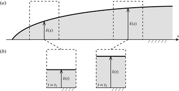
Figure 1(a) provides a sketch of the spatially developing boundary layer, where the boundary layer thickness
 ${\it\delta}$
, taken to be the 99 % thickness throughout, grows with streamwise coordinate
 $x$
. Below it in figure 1(b) we present the proposed temporally developing boundary layer, shown at two different instances in time. The shortened domain uses periodic boundary conditions in the streamwise direction, therefore the boundary layer thickness
 ${\it\delta}$
is forced to take the same value along the streamwise dimension, that is, there is no streamwise growth in the boundary layer – it may only grow upwards in time. For the spatially developing boundary layer
 $\text{d}{\it\delta}/\text{d}x$
decreases with increasing
 $Re_{x}$
, hence we might intuitively assume that the approximation represented by the temporal set-up improves with time. This is consistent with the idea that the parallel-flow approximation for the spatially developing boundary layer becomes better with increasing
 $Re_{x}=U_{\infty }x/{\it\nu}$
, where
 $U_{\infty }$
is the free-stream velocity,
 $x$
is the streamwise distance and
 ${\it\nu}$
is the kinematic viscosity. Note that the set-up in figure 1 with a flow over a stationary plate has been shown for ease of comparison with this most familiar of cases; the rest of this work will address a reversed set-up where the wall is moving and the free stream is at rest.
Comparison between the (a) spatially and (b) temporally developing boundary layers.

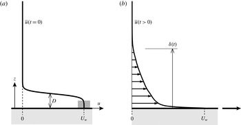
Illustration showing the streamwise velocity profile at (a)
 $t=0$
and (b)
 $t>0$
.
 $D$
is the ‘trip-wire’ diameter. The grey shaded area on the profile represents the magnitude and location of the white noise added to trigger transition.

An important difference between the spatially developing and the temporally developing boundary layers is exposed by comparing their respective momentum integral equations. Consider the Navier–Stokes equations governing incompressible flow for a fluid with density
 ${\it\rho}$
,
 $$\begin{eqnarray}\frac{\partial u_{i}}{\partial t}+\frac{\partial (u_{j}u_{i})}{\partial x_{j}}=-\frac{1}{{\it\rho}}\frac{\partial p}{\partial x_{i}}+{\it\nu}\frac{\partial ^{2}u_{i}}{\partial x_{j}^{2}},\quad \frac{\partial u_{j}}{\partial x_{j}}=0,\end{eqnarray}$$
which represent the momentum and continuity equations. We will take
 $x_{1}$
,
 $x_{2}$
and
 $x_{3}$
(or
 $x$
,
 $y$
and
 $z$
) to mean the streamwise, spanwise and wall-normal directions. We choose the frame of reference in which the wall (
 $z=0$
) is moving at constant velocity (
 $u=U_{w}$
) whilst the the far field (
 $z\rightarrow \infty$
) remains at rest (
 $u\rightarrow 0$
). This ‘conveyer-belt’ set-up is the well-known Rayleigh problem or Stokes’ first problem as shown in figure 2(b). The appropriate Reynolds decomposition for the temporally developing turbulent boundary layer is given by
 $u_{i}=\overline{u}(z,t){\it\delta}_{i1}+u_{i}^{\prime }(x,y,z,t)$
, where
 $\overline{(\cdot )}$
indicates averaging in the homogeneous
 $xy$
-plane. Substituting this decomposition in (1.1) and averaging in the homogeneous plane, we obtain
 $$\begin{eqnarray}\frac{\partial \overline{u}}{\partial t}={\it\nu}\frac{\partial ^{2}\overline{u}}{\partial z^{2}}-\frac{\partial (\overline{w^{\prime }u^{\prime }})}{\partial z}.\end{eqnarray}$$
In contrast, in the absence of a pressure gradient, recall that a similar analysis for the spatially developing boundary layer yields
 $$\begin{eqnarray}\overline{u}\frac{\partial \overline{u}}{\partial x}+\overline{w}\frac{\partial \overline{u}}{\partial z}={\it\nu}\frac{\partial ^{2}\overline{u}}{\partial z^{2}}-\frac{\partial (\overline{w^{\prime }u^{\prime }})}{\partial z}-\frac{\partial (\overline{u^{\prime 2}}-\overline{w^{\prime 2}})}{\partial x}.\end{eqnarray}$$
Since the difference in normal Reynolds stresses
 $\partial (\overline{u^{\prime 2}}-\overline{w^{\prime 2}})/\partial x$
is often neglected for further analysis of the spatially developing turbulent boundary layer, the difference between the two cases therefore amounts to a different left-hand side. Integrating (1.2) from the wall to the quiescent far field and imposing appropriate boundary conditions for the viscous and Reynolds stresses, we obtain
 $$\begin{eqnarray}\frac{\text{d}{\it\delta}^{\ast }}{\text{d}X}=\frac{1}{2}\frac{{\it\tau}_{0}}{\frac{1}{2}{\it\rho}U_{w}^{2}}\equiv \frac{C_{f}}{2}=\frac{u_{{\it\tau}}^{2}}{U_{w}^{2}}=\frac{1}{(U_{w}^{+})^{2}},\end{eqnarray}$$
where
 ${\it\delta}^{\ast }\equiv \int _{0}^{\infty }(\overline{u}/U_{w})\,\text{d}z$
, the displacement thickness,
 $X=U_{w}t$
, the temporal counterpart to
 $x$
in the spatially developing boundary layer,
 ${\it\tau}_{0}\equiv -{\it\mu}\,\partial \overline{u}/\partial z|_{0}>0$
, the wall shear stress and
 $u_{{\it\tau}}\equiv \sqrt{{\it\tau}_{0}/{\it\rho}}$
is the friction velocity. The definition of the displacement thickness here differs from the usual
 ${\it\delta}^{\ast }\equiv \int _{0}^{\infty }(1-\overline{u}/U_{\infty })\,\text{d}z$
due to the moving-wall frame of reference used in our set-up. For comparison, recall that the analogous expression for the spatially developing boundary layer is given by
 $\text{d}{\it\theta}/\text{d}x=C_{f}/2$
, where
 ${\it\theta}$
is the momentum thickness, defined by
 ${\it\theta}\equiv \int _{0}^{\infty }\overline{u}/U_{\infty }(1-\overline{u}/U_{\infty })\,\text{d}z$
. The preceding analysis suggests that
 ${\it\delta}^{\ast }$
plays an important role in the temporally developing turbulent boundary layer.
1.2 Resistance laws
We now develop resistance laws that will be used for setting up the simulations. The analysis assumes Coles’ law of the wall/wake for the turbulent boundary layer (Coles Reference Coles1956):
 $$\begin{eqnarray}\frac{U_{w}-\overline{u}}{u_{{\it\tau}}}=\frac{1}{{\it\kappa}}\log \left(\frac{zu_{{\it\tau}}}{{\it\nu}}\right)+A+\frac{{\it\Pi}}{{\it\kappa}}w\left(\frac{z}{{\it\delta}}\right),\end{eqnarray}$$
where
 ${\it\delta}={\it\delta}_{99}$
the
 $99\,\%$
boundary layer thickness,
 $w(z/{\it\delta})$
is Coles’ wake function,
 ${\it\Pi}$
measures the wake strength and
 ${\it\kappa}$
and
 $A$
are the log-law constants. From the definition of the displacement thickness and outer-layer similarity, we arrive at:
 $$\begin{eqnarray}\frac{{\it\delta}^{\ast }}{{\it\delta}}=C_{1}\frac{u_{{\it\tau}}}{U_{w}}=\frac{C_{1}}{U_{w}^{+}},\end{eqnarray}$$
as shown in Coles (Reference Coles1954), where
 $U_{w}^{+}\equiv U_{w}/u_{{\it\tau}}$
and
 $C_{1}$
is a constant, defined as
 $$\begin{eqnarray}C_{1}=\int _{0}^{\infty }\frac{\overline{u}}{u_{{\it\tau}}}\text{d}{\it\eta},\end{eqnarray}$$
where
 ${\it\eta}=z/{\it\delta}$
. Subjecting the wake function
 $w(z/{\it\delta})$
to normalising conditions
 $w(0)=0$
,
 $w(1)=2$
and
 $\int _{0}^{2}(z/{\it\delta})(w)\,\text{d}w=1$
, this constant may be written as
 $C_{1}=(1+{\it\Pi})/{\it\kappa}$
following Coles (Reference Coles1956). We seek an expression for
 $U_{w}^{+}=U_{w}^{+}(Re_{X})$
. The following repeats the analysis of Coles (Reference Coles1954). To this end, we first rearrange (1.5) written at
 $z={\it\delta}$
to obtain
 $$\begin{eqnarray}Re_{{\it\tau}}\equiv u_{{\it\tau}}\,{\it\delta}/{\it\nu}=\exp ({\it\kappa}[U_{w}^{+}-{\it\phi}(1)])\end{eqnarray}$$
or
 $$\begin{eqnarray}Re_{{\it\delta}}\equiv U_{w}{\it\delta}/{\it\nu}=U_{w}^{+}\exp ({\it\kappa}[U_{w}^{+}-{\it\phi}(1)]),\end{eqnarray}$$
where we use the shorthand,
 ${\it\phi}(1)=A+w(1)({\it\Pi}/{\it\kappa})=A+2{\it\Pi}/{\it\kappa}$
. Rewriting the left-hand side of (1.9) as
 $({\it\delta}/{\it\delta}^{\ast })Re_{{\it\delta}^{\ast }}$
, using (1.6), then substituting in (1.4) and invoking the change of variables that replaces
 $Re_{{\it\delta}^{\ast }}(Re_{X})$
with
 $Re_{{\it\delta}^{\ast }}(U_{w}^{+}(Re_{X}))$
, we arrive at the following expression:
 $$\begin{eqnarray}\frac{1}{(U_{w}^{+})^{2}}=\frac{\text{d}}{\text{d}U_{w}^{+}}\left[C_{1}\exp ({\it\kappa}[U_{w}^{+}-{\it\phi}(1)])\right]\frac{\text{d}U_{w}^{+}}{\text{d}Re_{X}}.\end{eqnarray}$$
Carrying out the differentiation with respect to
 $U_{w}^{+}$
as written and then integrating by parts gives
 $$\begin{eqnarray}Re_{X}=C_{1}\text{e}^{{\it\kappa}[U_{w}^{+}-{\it\phi}(1)]}\left[(U_{w}^{+})^{2}-\frac{2U_{w}^{+}}{{\it\kappa}}+\frac{2}{{\it\kappa}^{2}}\right]-\frac{2}{{\it\kappa}^{2}}C_{1}\text{e}^{-{\it\kappa}{\it\phi}(1)},\end{eqnarray}$$
where the initial condition
 $U_{w}^{+}(Re_{X}=0)=0$
is assumed. For
 ${\it\theta}\equiv \int _{0}^{\infty }\overline{u}/U_{w}(1-\overline{u}/U_{w})\,\text{d}z$
and using outer-layer similarity, it can also be shown that
 $$\begin{eqnarray}\frac{{\it\theta}}{{\it\delta}}=\frac{C_{1}}{U_{w}^{+}}-\frac{C_{2}}{(U_{w}^{+})^{2}},\end{eqnarray}$$
where
 $C_{2}$
is another constant, defined as
 $$\begin{eqnarray}C_{2}=\int _{0}^{\infty }\left(\frac{\overline{u}}{u_{{\it\tau}}}\right)^{2}\text{d}{\it\eta}.\end{eqnarray}$$
Then by using (1.9) we may write an expression for
 $Re_{{\it\theta}}$
as a function of
 $U_{w}^{+}$
:
 $$\begin{eqnarray}Re_{{\it\theta}}\equiv U_{w}{\it\theta}/{\it\nu}=\left(\frac{C_{1}}{U_{w}^{+}}-\frac{C_{2}}{(U_{w}^{+})^{2}}\right)U_{w}^{+}\exp ({\it\kappa}[U_{w}^{+}-{\it\phi}(1)]).\end{eqnarray}$$
2 Simulation set-up
The present code has been validated in Chung, Monty & Ooi (Reference Chung, Monty and Ooi2014). The domain size,
 $(L_{x},L_{y},L_{z})$
, is determined by the largest boundary layer thickness,
 ${\it\delta}_{f}$
, which occurs at the end of the simulation (the subscript
 $f$
refers to final). An important step in setting up the simulations is accurately predicting the final boundary layer thickness for a desired final Reynolds number, or alternatively to halt the simulation when the boundary layer ‘outgrows’ the domain. For this purpose we made use of relations from § 1.2 above. Following the work of Lozano-Durán & Jiménez (Reference Lozano-Durán and Jiménez2014), we set the wall-parallel domain size to
 $L_{x}=2{\rm\pi}{\it\delta}_{f}$
, and the spanwise domain size to
 $L_{y}={\rm\pi}{\it\delta}_{f}$
. Following Schlatter & Örlü (Reference Schlatter and Örlü2010), we set the wall-normal domain size to
 $L_{z}=3\,{\it\delta}_{f}$
.
In contrast, the grid spacing,
 $({\rm\Delta}x,{\rm\Delta}y,{\rm\Delta}z)$
, is determined by the smallest wall unit,
 ${\it\nu}/u_{{\it\tau},p}$
, which occurs earlier in the simulation when the skin friction reaches its maximum (the subscript
 $p$
refers to peak). The wall-normal grid spacing obeys a half-cosine mapping, giving a finer grid at the wall and a coarser grid away from it. Setting the coarsest grid spacing at the top of the domain
 ${\rm\Delta}z_{t}^{+}\approx 10$
, this cosine mapping results in the first wall-normal grid spacing
 ${\rm\Delta}z_{1}^{+}<0.2$
at all times. Grid spacing is uniform in both the streamwise and spanwise directions. The simulation of Moser, Kim & Mansour (Reference Moser, Kim and Mansour1999) guides the choice in grid points, in order to maintain
 ${\rm\Delta}x^{+}<9.7$
and
 ${\rm\Delta}y^{+}<4.8$
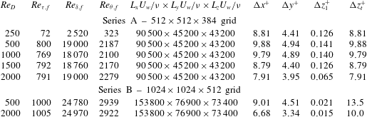
for the duration of the simulation. The grid spacings in wall units are monitored to ensure that the simulation is resolved at all times. More details regarding the calculation of domain size and grid spacing can be found in Kozul & Chung (Reference Kozul, Chung, Chowdhury and Alam2014). Table 1 summarises grid parameters. The grid spacings noted are the coarsest observed over the duration of the simulations, occurring toward the beginning where there is a peak in skin friction.
Simulation parameters for the present temporally developing boundary layer simulations. Domain dimensions are given in terms of
 ${\it\nu}/U_{w}$
, which can be arbitrarily chosen. The grid spacings in wall units are the coarsest observed over the duration of the simulation for each trip Reynolds number,
 $Re_{D}$
, occurring at the peak in
 $C_{f}$
toward the beginning of the simulation. The wall-normal grid spacings,
 ${\rm\Delta}z_{t}$
and
 ${\rm\Delta}z_{1}$
, correspond, respectively, to those at the top and the bottom of the domain. The grid is set up such that
 ${\rm\Delta}x\approx {\rm\Delta}z_{t}$
for series A.

Crucially, the boundary condition in the streamwise direction
 $x$
is periodic. Additionally, periodic boundary conditions are used for the spanwise
 $y$
direction. No-slip and impermeable boundary conditions representing a moving wall,
 $u=U_{w}$
and
 $v=w=0$
, are imposed at the bottom boundary (
 $z=0$
). The top boundary (
 $z=L_{z}$
) is a fixed wall, where no-slip and impermeable boundary conditions are also applied,
 $u=v=w=0$
. The pressure gradient is set to zero which is trivial for this set-up given the periodic streamwise boundary condition. In contrast, enforcing
 $\text{d}\overline{p}/\text{d}x=0$
in the spatial case requires non-trivial suction at the top boundary in order to ensure mass conservation (see Wu & Moin Reference Wu and Moin2009; Jiménez et al.
Reference Jiménez, Hoyas, Simens and Mizuno2010).
The computational set-up is that for a Couette flow simulation. If we let the simulation run indefinitely, we would have a fully developed Couette flow. However, we monitor the skin friction coefficient
 $C_{f}$
at the top wall relative to that at the bottom and terminate the simulation before the flow begins to ‘feel’ the top wall. The top wall
 $C_{f}$
remains at least five orders of magnitude smaller than the skin friction coefficient at the moving wall at every point in time and for all simulations presented in this work.
We are required to set initial conditions for the simulation. For this purpose, we take inspiration from the wall-mounted wire trips often employed by experimentalists. We seek to replicate the momentum deficit that is found directly after such a trip and more importantly its function in triggering a transition to a turbulent regime. The exact transition mechanism is not within the scope of the current work, however, we refer the interested reader to the large body of research that exists to study such questions (i.e. Gaster & Grant Reference Gaster and Grant1975; Narasimha Reference Narasimha1985; Rist & Fasel Reference Rist and Fasel1995).
We set
 $u_{i,0}=\overline{u}_{i,0}(z)+u_{i,0}^{\prime }(x,y,z)$
, where
 $$\begin{eqnarray}\overline{u}_{0}(z)=\frac{U_{w}}{2}+\frac{U_{w}}{2}\tanh \left[\frac{D}{2{\it\theta}_{sl}}\left(1-\frac{z}{D}\right)\right],\end{eqnarray}$$
for the streamwise initial velocity profile (cf. da Silva & Pereira Reference da Silva and Pereira2008), as well as
 $\overline{v}_{0}=\overline{w}_{0}=0$
as initial conditions. Physically, such an initial velocity profile resembles the wake of a wall-mounted trip wire with diameter,
 $D$
, and may be compared to physical trips placed at the beginning of a boundary layer wind tunnel. A similar initial velocity profile is found in the tow-tank experiment of Lee et al. (Reference Lee, Kwon, Monty, Hutchins, Brandner and Pearce2014), where the trip wire was pulled through the flow, leaving a shear layer in its wake. Hereafter, we will refer to
 $Re_{D}\equiv DU_{w}/{\it\nu}$
as the trip Reynolds number. The step-function-like shape of the
 $\tanh$
profile also means that the trip diameter can be identified with the initial boundary layer displacement thickness, that is,
 $D\approx {\it\delta}_{0}^{\ast }$
. It is important to note that if
 $Re_{D}$
is below some critical value, transition to a turbulent regime will not occur.
The momentum thickness of the shear layer is set to
 ${\it\theta}_{sl}\approx 54\,{\it\nu}/U_{w}$
. The Strouhal number of the primary Kelvin–Helmholtz instability is given by
 $S_{sl}\equiv f_{sl}{\it\theta}_{sl}/(U_{w}/2)\approx 0.033$
(e.g. da Silva & Pereira Reference da Silva and Pereira2008), from which the associated instability length scale is
 ${\it\lambda}_{sl}=(U_{w}/2)/f_{sl}$
. Therefore the number of Kelvin–Helmholtz rollers that form in our boundary layer from the inflectional profile can be estimated by
 $L_{x}/{\it\lambda}_{sl}\approx 0.033\,L_{x}/{\it\theta}_{sl}\approx 55.3$
. The small size of these rollers ensure that they will be quickly forgotten as time progresses, leading to a natural development at the earliest possible time. Finally, to trigger transition, white noise,
 $|u_{i,0}^{\prime }|<0.1\,U_{w}$
, is added to all velocity components near the wall where
 $U_{w}-\overline{u}_{0}<10^{-2}U_{w}$
(see figure 2
a).
Series A is a smaller domain size, planned for a final
 $Re_{{\it\tau}}\approx 590$
so as to be comparable to the channel flow of Moser et al. (Reference Moser, Kim and Mansour1999). It allows for rapid simulation and thus a parametric study of the trip Reynolds number
 $Re_{D}$
. The purpose of a larger domain size for series B is twofold. We wish to both study the effect of domain size, and the persistence of the impact of the initial trip on the flow at higher Reynolds number (i.e. for the largest
 $Re_{D}\approx 2000$
). Planned for a larger
 $Re_{{\it\tau}}\approx 1000$
, it is vastly more computationally demanding and is thus used only for two indicative trip Reynolds numbers to address both matters.
3 Results
The transport of a passive scalar
 $c$
with Schmidt number of
 $Sc=1$
allows us to visualise the flow. For symmetry with the streamwise velocity field, the scalar takes the same boundary values as the streamwise velocity, that is,
 $C_{w}=1$
and
 $C_{\infty }=0$
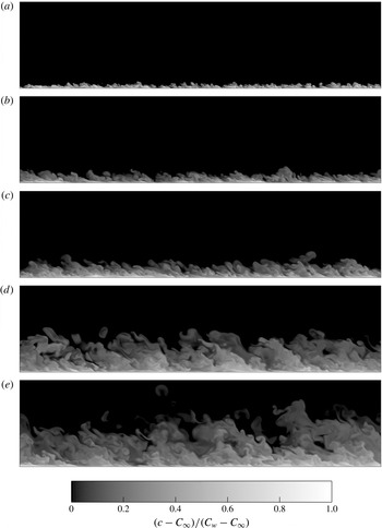
. Figure 3 shows snapshots throughout the simulation for the
 $Re_{D}\approx 500$
(series B) case offering a first view of the set-up. The visualisations show many similarities with the well-known structures of the spatial boundary layer. We are able to identify both large-scale motions and ‘typical eddies’ as depicted by figure 1(b) in Falco (Reference Falco1977). We too find that the non-turbulent regions persist deep into the boundary layer. Eddy structures resembling the hairpins and bulges marked on figure 2(a) of Adrian (Reference Adrian2007) are also discernible.
Scalar for
 $Re_{D}\approx 500$
(series B) at (a–e)
 $Re_{{\it\theta}}=337,~555,~861,~2007,~2939$
(
 $Re_{{\it\tau}}=144,~241,~340,~720,~1000$
). The wall is moving to the right.

Visualisations such as those shown in figure 3 for the different cases suggest the exact mode of transition depends on
 $Re_{D}$
(e.g. for the larger trip Reynolds numbers
 $Re_{D}=1000$
, 1500 and 2000, similar snapshots of the scalar field clearly show the formation of Kelvin–Helmholtz rollers). However, we are here principally concerned with how trip Reynolds number
 $Re_{D}$
impacts upon the development of statistics at a later point in time (‘downstream’). Results related to the scalar will be addressed in § 6. The simulations of series A are run somewhat beyond the planned-for
 $Re_{{\it\tau}}=590$
, reaching
 $Re_{{\it\tau}}\approx 800$
. This results in smaller domain sizes at the end of this set of simulations (
 $L_{x}/{\it\delta}_{f}\approx 4.5$
) than planned (
 $L_{x}/{\it\delta}_{f}\approx 6.0$
).
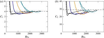
(a)
 $C_{1}$
as a function of
 $Re_{{\it\theta}}$
calculated using (1.6); series A in solid lines: —— (black),
 $Re_{D}\approx 500$
; —— (blue),
 $Re_{D}\approx 1000$
; —— (orange),
 $Re_{D}\approx 1500$
; —— (green),
 $Re_{D}\approx 2000$
; series B in dashed lines: – - – - (black),
 $Re_{D}\approx 500$
; – - – - (green),
 $Re_{D}\approx 2000$
; thin horizontal dashed line, at
 $C_{1}=4.05$
; (b)
 $C_{2}$
as a function of
 $Re_{{\it\theta}}$
using (1.6) and (1.12); thin horizontal dashed line, at
 $C_{2}=29.0$
.

In order to make use of the resistance laws developed in § 1.2, the constants introduced for the problem must be established. Values for
 ${\it\kappa}=0.384$
and
 $A=4.173$
are set following the compilation of Nagib, Chauhan & Monkewitz (Reference Nagib, Chauhan and Monkewitz2007). The time history of
 $U_{w}^{+}\,{\it\delta}^{\ast }/{\it\delta}$
in (1.6) reveals that the value of
 $C_{1}$
stabilises well after transition as shown in figure 4(a) and being very similar to the value of Coles (Reference Coles1954) it is set to that value of
 $4.05$
. Similarly, using (1.12), we are also able to plot the evolution of
 $C_{2}$
as shown in figure 4(b). The relation of Coles (Reference Coles1956) then allows us to deduce
 ${\it\Pi}={\it\kappa}C_{1}-1\approx 0.55$
which is the same as that given in Coles (Reference Coles1956). This value of
 ${\it\Pi}$
found from the definition of
 $C_{1}$
is also verified graphically for our simulation from the outer-scaled velocity defect profile. We can then calculate
 ${\it\phi}(1)=A+2{\it\Pi}/{\it\kappa}\approx 7.1$
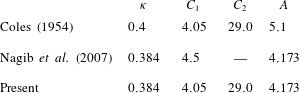
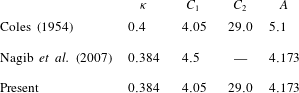
. The relevant constants used for this simulation are noted in table 2, where they are compared against those of Coles (Reference Coles1954) and Nagib et al. (Reference Nagib, Chauhan and Monkewitz2007). All subsequent plots will use those constants labelled ‘Present’, unless otherwise specified.
Comparison of constants obtained from the present temporally developing boundary layer simulations.
3.1 Bulk and first-order statistics
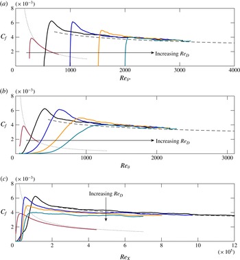
Variation of skin friction coefficient versus (a)
 $Re_{{\it\delta}^{\ast }}$
, (b)
 $Re_{{\it\theta}}$
and (c)
 $Re_{X}$
: —— (brown),
 $Re_{D}\approx 250$
; —— (black),
 $Re_{D}\approx 500$
; —— (blue),
 $Re_{D}\approx 1000$
; —— (orange),
 $Re_{D}\approx 1500$
; —— (green),
 $Re_{D}\approx 2000$
; – – –, turbulent resistance law (1.11);
 $\cdots \cdots$
, laminar resistance law.

Figure 5 shows the development of
 $C_{f}=2/(U_{w}^{+})^{2}$
versus
 $Re_{{\it\theta}}$
,
 $Re_{X}$
and
 $Re_{{\it\delta}^{\ast }}$
with the five different trip Reynolds numbers
 $Re_{D}$
for series A. The skin friction coefficient is zero to machine precision for the first few iterations of the simulation. We are able to now examine how the turbulent resistance laws developed in § 1.2 perform against the data. Given that
 $C_{f}$
is a function of
 $U_{w}^{+}$
only, we are able to plot it against expressions for
 $Re_{{\it\delta}^{\ast }}(U_{w}^{+})$
,
 $Re_{{\it\theta}}(U_{w}^{+})$
and
 $Re_{X}(U_{w}^{+})$
given by (1.11) and other similar relations. We are therefore able to plot these predictive curves for a chosen range of
 $U_{w}^{+}$
. Here we begin them at
 $U_{w}^{+}\approx 20$
, roughly where our simulations have transitioned, and extend them beyond the span of the data. We also plot the laminar branch of
 $C_{f}$
derived from the well-known
 $\text{erfc}$
profile. Figure 5 suggests that, provided the trip is large enough to trigger transition to turbulence, the temporal development of the turbulent boundary layer as measured by
 $C_{f}$
eventually collapses to a natural evolution independent of the initial
 $Re_{D}$
. When
 $Re_{D}\lesssim 250$
, the perturbations are not strong enough to result in transition to a turbulent regime, however for
 $Re_{D}\gtrsim 500$
they are. A useful comparison is with the tow-tank experiment of Lee et al. (Reference Lee, Kwon, Monty, Hutchins, Brandner and Pearce2014) which made use of a trip Reynolds number of
 $Re_{D}\approx 870$
. Provided transition is initiated, the flow that is least perturbed (smallest
 $Re_{D}$
) leads to a natural or undisturbed development from the smallest possible
 $Re_{{\it\theta}}$
. This can be observed in figure 5(a,b), where first the
 $Re_{D}\approx 1000$
curve, then the
 $Re_{D}\approx 1500$
curve and finally the
 $Re_{D}\approx 2000$
curve, track the
 $Re_{D}\approx 500$
curve. Convincing collapse of
 $C_{f}$
is best observed with
 $Re_{{\it\delta}^{\ast }}$
, in agreement with the analysis in the Introduction, although a fair collapse of
 $C_{f}$
is also observed with
 $Re_{{\it\theta}}$
. We do not observe convincing collapse in figure 5(c) with
 $Re_{X}$
owing to the ill-defined virtual origin. Recall that the initial condition
 $U_{w}^{+}(Re_{X}=0)=0$
is used in the derivation leading to (1.11). However, we expect to see collapse if we allow for a simple shift in
 $Re_{X}$
by
 $Re_{X,0}$
. In any case, the virtual-origin effect becomes unimportant at large
 $Re_{X}$
because
 $Re_{X}-Re_{X,0}\sim Re_{X}$
. Despite this non-collapse, plotting as a function of
 $Re_{X}$
is important since this quantity is directly proportional to the time taken for the various simulations (
 $X=U_{w}t$
) and indicates the relative development of each case in time.
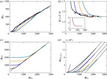
Evolution profiles for the trip study as a function of
 $Re_{{\it\theta}}$
: series A in solid lines: —— (brown),
 $Re_{D}\approx 250$
; —— (black),
 $Re_{D}\approx 500$
; —— (blue),
 $Re_{D}\approx 1000$
; —— (orange),
 $Re_{D}\approx 1500$
; —— (green),
 $Re_{D}\approx 2000$
; series B in dashed lines: – – – (black),
 $Re_{D}\approx 500$
; – – – (green),
 $Re_{D}\approx 2000$
; thin black lines are functions of
 $U_{w}^{+}$
as developed in § 1.2; spatially developing DNS data: ●, Schlatter et al. (Reference Schlatter, Örlü, Li, Brethouwer, Fransson, Johansson, Alfredsson and Henningson2009); ▴, Jiménez et al. (Reference Jiménez, Hoyas, Simens and Mizuno2010). For (d), a virtual origin is subtracted from the expression (1.11) to fit each
 $Re_{D}$
.

Evolution profiles are plotted in figure 6 for all five trip Reynolds numbers, that is (a)
 $Re_{{\it\tau}}$
, (b) shape factor
 $H$
, (c)
 $Re_{{\it\delta}^{\ast }}$
and (d)
 $Re_{X=U_{w}t}$
as a function of
 $Re_{{\it\theta}}$
. Reference curves from § 1.2 (functions of a range of
 $U_{w}^{+}$
on both axes) are plotted for all the profiles; for this purpose constants in table 2 (Present) are used. Figure 6(a) suggests that the
 $Re_{D}\approx 2000$
case has not yet collapsed with the others. This motivates a simulation with a larger domain size in order to continue this simulation for higher
 $Re_{{\it\theta}}$
, and discover the true ‘recovery’ time of this case. Curves for series B (dashed lines) for
 $Re_{D}\approx 500$
and
 $Re_{D}\approx 2000$
collapse very well however and give an indication of the magnitude of the scatter that might be expected in computing
 $Re_{{\it\tau}}$
. Indeed, curves for the other three plots shown in figure 6 are computed using only integral values, whereas plotting
 $Re_{{\it\tau}}$
requires the computation of the instantaneous
 $99\,\%$
boundary layer thickness
 ${\it\delta}$
, making this quantity more liable to scatter. It has been verified that it is not due to a spurious flow at the top of the box (i.e. a domain size effect). We find the largest difference between our simulation data and the curves developed in § 1.2 for shape factor
 $H$
in figure 6(b), however plotting spatially developing data by Schlatter et al. (Reference Schlatter, Örlü, Li, Brethouwer, Fransson, Johansson, Alfredsson and Henningson2009) and Jiménez et al. (Reference Jiménez, Hoyas, Simens and Mizuno2010) places this difference in context. To aid comparison, the vertical axis range for
 $H$
is the same as that in Nagib et al. (Reference Nagib, Chauhan and Monkewitz2007). Again reinforcing what we saw in the skin friction profiles, we find good collapse of
 $Re_{{\it\delta}^{\ast }}$
in figure 6(c). In figure 6(d), the curve for
 $Re_{X}(U_{w}^{+})$
is shifted for each
 $Re_{D}$
thus allowing the estimation of
 $Re_{X,0}$
, which is plotted against
 $Re_{D}$
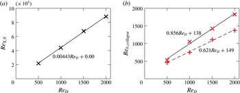
in figure 7(a). We find that it grows linearly with trip Reynolds number, which we expect following the proportional response of the flow to
 $Re_{D}$
.
(a) Virtual origin
 $Re_{X,0}$
versus trip Reynolds number
 $Re_{D}$
;
 $\times$
,
 $Re_{X,0}$
used in figure 6(d); ——, least-squares fit for
 $Re_{X,0}$
shown on figure; (b)
 $+$
, collapse of
 $u_{rms}^{+}$
contours at
 $z^{+}=10$
(same markers as shown on figure 10
a); – – –, least-squares fit for
 $Re_{{\it\theta},collapse}$
shown on figure;
 $\times$
, collapse of
 $u_{rms}^{+}$
contours at
 $z/{\it\delta}=0.15$
(same markers as shown on figure 10
c); ——, least-squares fit for
 $Re_{{\it\theta},collapse}$
shown on figure.

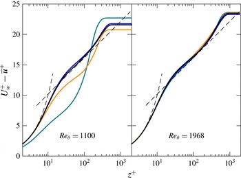
Mean streamwise velocity profile at two different
 $Re_{{\it\theta}}$
for series A: —— (black),
 $Re_{D}\approx 500$
; —— (blue),
 $Re_{D}\approx 1000$
; —— (orange),
 $Re_{D}\approx 1500$
; —— (green),
 $Re_{D}\approx 2000$
; – – –,
 $U_{w}^{+}-\overline{u}^{+}=z^{+}$
and
 $U_{w}^{+}-\overline{u}^{+}=(1/{\it\kappa})\log z^{+}+A$
with constants from table 2 (Present).

Mean profiles for the streamwise velocity are plotted in figure 8 for two different
 $Re_{{\it\theta}}$
, with dashed curves also plotted for reference identifying both the viscous sublayer and the logarithmic region, confirming that we have a turbulent boundary layer forming. For the logarithmic layer, the constants of Nagib et al. (Reference Nagib, Chauhan and Monkewitz2007) represent a good match with our mean streamwise velocity profile. For all statistics presented at specified Reynolds numbers in this work, profiles were averaged across time windows of
 ${\it\alpha}{\it\delta}/u_{{\it\tau}}$
where
 ${\it\alpha}=0.5$
is used to smooth the statistics and limit the effect of a single eddy on profiles of various quantities presented herein (see appendix A). In terms of development, these profiles corroborate the story told by the skin friction profiles shown in figure 5(b): the least perturbed boundary layer at
 $Re_{D}\approx 500$
is the case that assumes undisturbed development at the lowest
 $Re_{{\it\theta}}$
. At
 $Re_{{\it\theta}}=1100$
, the larger two trips (
 $Re_{D}\gtrsim 1500$
) have not yet tracked the other curves; later at the larger
 $Re_{{\it\theta}}=1968$
, both the
 $Re_{D}\approx 1500$
and
 $Re_{D}\approx 2000$
flows appear to have relaxed to a natural development for this first-order statistic.
3.2 Second-order statistics
3.2.1 Profiles
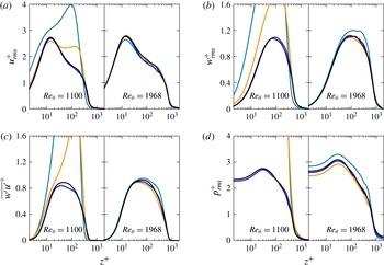
Turbulence statistics at
 $Re_{{\it\theta}}=1100$
and
 $Re_{{\it\theta}}=1968$
for trips
 $Re_{D}\approx 500$
and above are shown in figure 9. Despite the smoothing effect of the time-window averaging, it is clear that the
 $Re_{D}\approx 2000$
case in particular has not yet collapsed at the higher
 $Re_{{\it\theta}}=1968$
. Consistent with spatially developing boundary layers (Schlatter & Örlü Reference Schlatter and Örlü2012), we observe an earlier convergence in the mean profiles shown in figure 8 compared to the turbulent statistics, an effect clearly seen at
 $Re_{{\it\theta}}=1968$
for
 $Re_{D}\approx 2000$
.
Second-order statistics at two different
 $Re_{{\it\theta}}$
for series A: —— (black),
 $Re_{D}\approx 500$
; —— (blue),
 $Re_{D}\approx 1000$
; —— (orange),
 $Re_{D}\approx 1500$
; —— (green),
 $Re_{D}\approx 2000$
.

3.2.2 Contours of
 $u_{rms}^{+}$

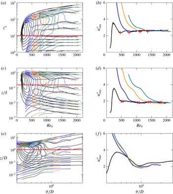
To further quantify the extent to which initial conditions hasten or delay collapse to a natural evolution, contours of constant root-mean-squared values of the streamwise velocity fluctuations (
 $u_{rms}^{+}$
) are plotted in figure 10(a) following the example of Schlatter & Örlü (Reference Schlatter and Örlü2012). As expected, we find collapse of the inner region at higher Reynolds numbers by plotting with
 $z^{+}$
on the vertical scale. Such contours provide us with a ‘map’ in time from which we are able to estimate which Reynolds number must be attained for various cases to relax to an undisturbed state that does not ‘remember’ its original trip Reynolds number
 $Re_{D}$
. Scaling the vertical axis by
 ${\it\delta}$
collapses the outer region, yet we see that the contours only become aligned at the highest Reynolds numbers shown at the right. Horizontal cuts are taken through the contours at
 $z^{+}=10$
in figure 10(a) and at
 $z/{\it\delta}=0.15$
in figure 10(c). The resulting cross-sections are shown in figures 10(b) and 10(d). Markers are placed where we estimate that the
 $u_{rms}^{+}$
profiles have collapsed, and these are plotted against
 $Re_{D}$
in figure 7(b). We find a convincing linear relationship, that is, the
 $Re_{{\it\theta}}$
required to ensure collapse scales linearly with trip Reynolds number
 $Re_{D}$
. We find that a slightly higher Reynolds number must be achieved to ensure collapse in the outer layer.
Contours of constant root-mean-squared values of the streamwise velocity fluctuations (
 $u_{rms}^{+}$
) for series A in steps of
 ${\rm\Delta}u_{rms}^{+}=0.5$
: (a) as a function of
 $Re_{{\it\theta}}$
; (b) cross-section of (a) at
 $z^{+}=10$
with markers at collapse the same as those on figure 7(b); (c) same as (a) but scaled with
 ${\it\delta}$
on the vertical axis; (d) cross-section of (c) at
 $z/{\it\delta}=0.15$
with markers at collapse the same as those on figure 7(b); (e) same as (a) but scaled with trip height
 $D$
along the horizontal and vertical axis; (f) cross-section of (e) at
 $z/D=1$
; —— (black),
 $Re_{D}\approx 500$
; —— (blue),
 $Re_{D}\approx 1000$
; —— (orange),
 $Re_{D}\approx 1500$
; —— (green),
 $Re_{D}\approx 2000$
.

Scaling the horizontal and vertical axis by
 $D$
as shown in figure 10(e) causes the contours from the different cases to be more aligned, particularly in the outer region, although we note that the
 $Re_{D}\approx 500$
case (black curves) suggests an alternate route to transition. A cross-sectional cut at
 $z/D=1$
confirms this suspicion, although the curves do not differ excessively. It may be more pertinent to consider which universal value of
 ${\it\theta}/D$
must be obtained to be confident that all simulations have converged to a similar behaviour. Intuitively, the larger the initial disturbance or trip, the longer the flow will take to recover and ‘forget’ its initial conditions.
We propose a relative indicator of
 ${\it\theta}/D\approx 1$
, below which the effect of the trip is strongly felt, suggested by the clear collapse of
 $u_{rms}^{+}$
with
 ${\it\theta}/D$
at fixed
 $z/D$
(except
 $Re_{D}\approx 500$
). Translated to a wind tunnel drawing air, this implies that for a trip wire of
 ${\approx}1~\text{mm}$
with
 $U_{\infty }\approx 20~\text{m}~\text{s}^{-1}$
and a kinematic viscosity of air around
 ${\it\nu}\approx 1.5\times 10^{-5}~\text{m}^{2}~\text{s}^{-1}$
, giving
 $Re_{D}\approx 1300$
, that one would have to wait until
 $Re_{{\it\theta}}\approx 1300$
for the flow to no longer be dictated by its specific initial trip. From figure 6(d) we can graphically estimate that
 $Re_{X}\approx 8\times 10^{5}$
at this
 $Re_{{\it\theta}}$
(assuming no virtual origin), which translates to measuring
 ${\approx}0.6~\text{m}$
downstream of the trip. This generalises the previous work of Schlatter & Örlü (Reference Schlatter and Örlü2012) that suggests if transition is effected inside the boundary layer at
 $Re_{{\it\theta}}<300$
, all quantities agree well for
 $Re_{{\it\theta}}>2000$
. Such a metric may prove useful in situations where a very large initial trip is employed.
3.3 Higher-order statistics
Skewness and flatness of the streamwise velocity are plotted in figure 11 for the trip study (series A) at
 $Re_{{\it\theta}}=1100$
and
 $Re_{{\it\theta}}=1968$
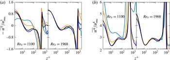
as for the other statistics. All of the cases appear to have collapsed fairly well at the higher Reynolds number, although there is some scatter, in particular at the wall for the fourth-order flatness,
 $K$
, shown in figure 11(b). Although these profiles have been time-window averaged, we do not have converged statistics since there is only one realisation of the temporal simulation.
(a) Streamwise velocity skewness (negative sign due to the reversed moving-wall reference frame) and (b) flatness at two different
 $Re_{{\it\theta}}$
for series A: —— (black),
 $Re_{D}\approx 500$
; —— (blue),
 $Re_{D}\approx 1000$
; —— (orange),
 $Re_{D}\approx 1500$
; —— (green),
 $Re_{D}\approx 2000$
.

Streamwise spectra at (a–d)
 $z^{+}=10$
and at (e–h)
 $z/{\it\delta}=0.15$
for the trip study (series A) at two different
 $Re_{{\it\theta}}$
: —— (black),
 $Re_{D}\approx 500$
; —— (blue),
 $Re_{D}\approx 1000$
; —— (orange),
 $Re_{D}\approx 1500$
; —— (green),
 $Re_{D}\approx 2000$
.

3.4 Spectra
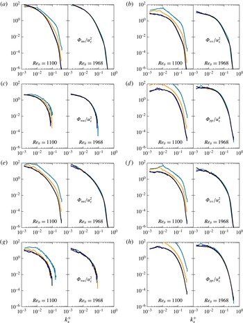
In figure 12 we plot streamwise energy spectra, normalised such that
 $\int _{0}^{\infty }{\it\Phi}_{uu}(k_{x})\,\text{d}k_{x}=u_{rms}^{2}$
, for the trip study (series A) at the same two wall-normal locations where cross-sectional cuts were taken through the contours of
 $u_{rms}^{+}$
in figure 10: in (a–d) at
 $z^{+}=10$
and in (e–h) at
 $z/{\it\delta}=0.15$
. Plotted at two Reynolds numbers, these figures demonstrate the different rate of collapse of various scales depending on trip Reynolds number
 $Re_{D}$
. At the earlier
 $Re_{{\it\theta}}=1100$
, we find that all scales have already collapsed at the two distances
 $z$
from the wall for the smaller
 $Re_{D}\approx 500$
and
 $1000$
, whereas the
 $Re_{D}\approx 2000$
case differs at all scales. However, at the larger
 $Re_{{\it\theta}}=1968$
, all scales for all trip Reynolds numbers have visibly collapsed. Note the limitations that our box places on spectra of larger scales (small wavenumber
 $k_{x}^{+}$
). This results in jagged lines for want of features over which to average. The spectra are somewhat smoother near the wall at
 $z^{+}=10$
than at
 $z/{\it\delta}=0.15$
, although collapse is already achieved for all
 $Re_{D}$
at the higher Reynolds number according to figure 7(b) (i.e.
 $Re_{{\it\theta},collapse}\approx 1800$
for largest trip
 $Re_{D}\approx 2000$
).
4 Impact of box size
Given the short length of our computational domain in the streamwise dimension, it is reasonable to question the impact of this on our flow, in particular with regards to larger structures. As mentioned earlier, the simulations for the trip study (series A) were continued beyond the planned
 $Re_{{\it\tau}}\approx 590$
to
 $Re_{{\it\tau}}\approx 800$
, resulting in a smaller domain size of
 $L_{x}/{\it\delta}\approx 4.5$
, compared to the planned
 $L_{x}/{\it\delta}\approx 6.0$
, although all profiles of statistics that are shown in this work are at an earlier point (i.e.
 $Re_{{\it\theta}}\approx 2000$
), where the domain is
 $L_{x}/{\it\delta}\geqslant 5.2$
, the exact value depending on the trip Reynolds number
 $Re_{D}$
.
The small domain clearly possesses a domain size that is below that recommended by Schlatter & Örlü (Reference Schlatter and Örlü2010) and Lozano-Durán & Jiménez (Reference Lozano-Durán and Jiménez2014), however we note that these guidelines are only breached toward the end of the small domain simulations, and a larger domain would not change the broad conclusions of the study. For example, considering figures 5 (skin-friction coefficient profiles), 6 (additional bulk statistics) and 10 (contour plots of
 $u_{rms}^{+}$
), we could indeed clip the figures at approximately
 $Re_{{\it\theta}}\approx 1800$
so as to abide by the guidelines on domain size, but it would not change any of the conclusions we make about the effect of the trip Reynolds number upon the flow and its recovery.
Two simulations with a larger domain size, planned for
 $Re_{{\it\tau}}\approx 1000$
, were undertaken for
 $Re_{D}\approx 500$
and
 $2000$
(series B) to investigate this issue. The number of grid points and box dimensions are scaled up with the new final
 $Re_{{\it\tau}}$
, compared to the previous
 $Re_{{\it\tau}}=590$
.
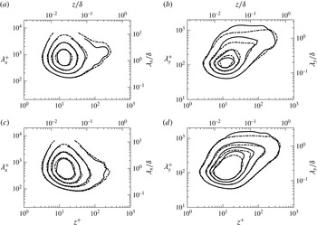
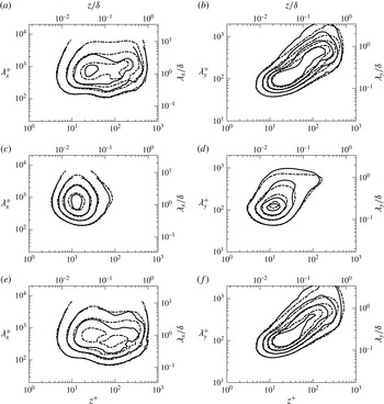
Contours of premultiplied one-dimensional energy spectra are plotted in figures 13 and 14 for the
 $Re_{D}\approx 500$
case from both series A and B in order to quantify the effect of box size on results. This is done at
 $Re_{{\it\tau}}=590$
to ensure that the small domain had here adhered to the aforementioned guidelines. Whereas at
 $Re_{{\it\tau}}=590$
the smaller simulation has a domain size of
 $L_{x}/{\it\delta}\approx 6.7$
, the larger simulation has a much bigger domain size of
 $L_{x}/{\it\delta}\approx 11.2$
. These figures clearly show that this larger domain affects the streamwise results more so than in the spanwise direction
 $y$
, whose contours are much the same regardless of domain size. This confirms that our smaller domain is able to faithfully capture the main dynamical features of the flow up to its planned
 $Re_{{\it\tau}}\approx 590$
. More precisely, since the premultiplied spectra of the two simulations are equivalent for
 ${\it\lambda}_{x}/{\it\delta}<0.6$
and
 ${\it\lambda}_{y}/{\it\delta}<0.3$
, the two flows are energetically similar in this region.
Premultiplied one-dimensional spectra of (a,b) streamwise velocity and (c,d) scalar for
 $Re_{D}\approx 500$
at
 $Re_{{\it\tau}}=590$
as a function of
 $z^{+}$
. For (a,c) plotted against streamwise wavelengths and for (b,d) against spanwise wavelengths: ——, series A (small domain); – - – -, series B (large domain). A Gaussian filter with
 ${\it\sigma}=1.5$
was used on the time-window averaged (see appendix A,
 ${\it\alpha}=0.5$
) data to smooth contour lines. Contour levels for each subfigure: (a)
 $k_{x}{\it\Phi}_{uu}/u_{{\it\tau}}^{2}=0.6$
, 1.0, 1.4, 1.8; (b)
 $k_{y}{\it\Phi}_{uu}/u_{{\it\tau}}^{2}=0.8$
, 1.6, 2.4, 3.2; (c)
 $k_{x}{\it\Phi}_{cc}/c_{{\it\tau}}^{2}=0.6$
, 1.0, 1.4, 1.8; (d)
 $k_{y}{\it\Phi}_{cc}/c_{{\it\tau}}^{2}=0.8$
, 1.6, 2.4, 3.2.

Premultiplied one-dimensional spectra of (a,b) streamwise–wall-normal velocities, (c,d) streamwise velocity–scalar and (e,f) wall-normal velocity–scalar for
 $Re_{D}\approx 500$
at
 $Re_{{\it\tau}}=590$
as a function of
 $z^{+}$
. For (a,c,e) plotted against streamwise wavelengths and for (b,d,f) against spanwise wavelengths: ——, series A (small domain); – - – -, series B (large domain). A Gaussian filter with
 ${\it\sigma}=1.5$
was used on the time-window averaged (see appendix A,
 ${\it\alpha}=0.5$
) data to smooth contour lines. Contour levels for each subfigure: (a)
 $k_{x}{\it\Phi}_{wu}/u_{{\it\tau}}^{2}=0.04$
, 0.11, 0.18, 0.25; (b)
 $k_{y}{\it\Phi}_{wu}/u_{{\it\tau}}^{2}=0.1$
, 0.2, 0.3, 0.4; (c)
 $k_{x}{\it\Phi}_{uc}/u_{{\it\tau}}c_{{\it\tau}}=0.6$
, 1.0, 1.4, 1.8; (d)
 $k_{y}{\it\Phi}_{uc}/u_{{\it\tau}}c_{{\it\tau}}=0.8$
, 1.6, 2.4, 3.2; (e)
 $k_{x}{\it\Phi}_{wc}/u_{{\it\tau}}c_{{\it\tau}}=0.04$
, 0.11, 0.18, 0.25; (f)
 $k_{y}{\it\Phi}_{wc}/u_{{\it\tau}}c_{{\it\tau}}=0.1$
, 0.2, 0.3, 0.4.

5 Comparison with the spatial turbulent boundary layer
Variation of skin friction coefficient versus
 $Re_{{\it\theta}}$
: thick solid line,
 $Re_{D}\approx 500$
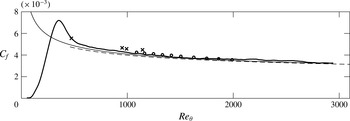
, series B; – – –, turbulent resistance law (1.11); thin solid line, Coles–Fernholz 2, relation from Nagib et al. (Reference Nagib, Chauhan and Monkewitz2007) (their constants);
 $\times$
, experimental data from Erm & Joubert (Reference Erm and Joubert1991) tripped by wire at the nearest
 $Re_{D}$
to our
 $Re_{D}\approx 500$
case (
 $U_{\infty }=8.0~\text{m}~\text{s}^{-1}$
); ○, spatially developing DNS by Jiménez et al. (Reference Jiménez, Hoyas, Simens and Mizuno2010).

This section will investigate how well the temporal boundary layer set-up models the spatially developing boundary layer, as proposed by the schematic shown in figure 1. In the following, we make use of data from series B (large domain). To begin with, the skin friction
 $C_{f}$
profile as a function of
 $Re_{{\it\theta}}$
is replotted in figure 15 for
 $Re_{D}\approx 500$
, that of the smallest trip Reynolds number which triggered transition to a turbulent regime and the case that collapsed at the earliest
 $Re_{{\it\theta}}$
. As before on figure 5(b), we plot
 $C_{f}=2/(U_{w}^{+})^{2}$
against the turbulent resistance law for
 $Re_{{\it\theta}}(U_{w}^{+})$
(1.14) developed in § 1.2 for an arbitrary range of
 $U_{w}^{+}$
. In addition we now also plot the well-known Coles–Fernholz relation from Nagib et al. (Reference Nagib, Chauhan and Monkewitz2007) for the spatially developing turbulent boundary layer. We find that it agrees well with our resistance law. Comparison with data for spatially developing turbulent boundary layers will allow us to further gauge the success of our model in this respect. Hence we plot both experimental data by Erm & Joubert (Reference Erm and Joubert1991) and the numerical data of the spatially developing DNS by Jiménez et al. (Reference Jiménez, Hoyas, Simens and Mizuno2010) and find that we have very good agreement with both.
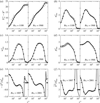
Furthermore, plotting profiles of various statistics at matched Reynolds numbers against data for spatially developing turbulent boundary layers reveals that our temporal model is a very good model for the spatially developing case. Previously, we had seen that the average streamwise velocity profiles of figure 8 suggested that we had a turbulent boundary layer forming, in the sense that we were clearly able to identify a linear viscous sublayer region as well as a limited logarithmic region. However, figure 16(a) now convincingly demonstrates that the temporal set-up yields the same mean streamwise velocity profile as the spatially developing case. We find excellent agreement in figure 16 at matched
 $Re_{{\it\theta}}$
with the data of Jiménez et al. (Reference Jiménez, Hoyas, Simens and Mizuno2010), a DNS of a spatially developing turbulent boundary layer. Yet, the agreement is not limited to first-order statistics, and we find excellent agreement for the second-order streamwise variance shown in figure 16(b), the third-order streamwise skewness in 16(c) and finally for the fourth-order streamwise flatness in 16(d), when the Reynolds number is correctly matched. Similar agreement is found for the remaining second-order statistics shown in figure 9. Interestingly, we find good agreement in the outer layer for all statistics shown, except for the streamwise skewness and flatness, which is to be expected given division by near-zero
 $u_{rms}$
in the free stream.
We can therefore conclude that the temporal model for the turbulent boundary layer has the potential to be a very useful tool for the study of turbulent boundary layers, given that we are able to convincingly reproduce profiles from spatially developing simulations up to fourth-order statistics. At present we are only able to assert this agreement for one-point statistics, and a separate study in the spirit of Sillero, Jiménez & Moser (Reference Sillero, Jiménez and Moser2014) would be required to make any conclusions about two-point statistics. It is likely that large velocity structures approaching the scale of the boundary layer thickness differ somewhat to that of the spatial boundary layer, both due to the boundary conditions imposed and the box dimensions. If the goal of a study is to obtain such one-point statistics, and one is satisfied with only humble convergence, the reduction in grid points translates into greatly reduced computational effort, as well as much smaller data files.
There are several caveats to keep in mind with regards to the temporal set-up. The profiles shown in this work for the temporal boundary layer are from a single realisation. For fully converged statistics, we would need to resimulate the case many times using a different random noise for each realisation, which would clearly negate some of the cost saving that was made in shortening the domain. This can be somewhat mitigated by window averaging, provided the window size
 $T$
is carefully chosen such that
 $Re_{{\it\tau}}$
does not vary significantly over the window. We emphasise here that the temporal set-up, using data from only one realisation, does not provide highly converged statistics. Rather, we believe that it could prove more useful in the study of the dynamics of turbulence (e.g. tracking the evolution of structures in time), since the temporal set-up provides an efficient means by which to access time-resolved data for the turbulent boundary layer. In the same way that flow structures have been studied in domains using a periodic streamwise boundary condition for pipes (Eggels et al.
Reference Eggels, Unger, Weiss, Westerweel, Adrian, Friedrich and Nieuwstadt1994) and channels (Abe, Kawamura & Choi Reference Abe, Kawamura and Choi2004), the temporal approach might be useful to study structures within the turbulent boundary layer.
Comparisons with the spatially developing turbulent boundary layer for various statistics. First order: (a) mean streamwise velocity profile. Second order: root-mean-squared velocity fluctuations, (b) streamwise, (c) wall normal; (d) root-mean-squared pressure fluctuations. Third order: (e) streamwise skewness. Fourth order: (f) streamwise flatness. Temporal simulation: thick solid line,
 $Re_{D}\approx 500$
, series B; data from spatial simulations: ○, DNS of Jiménez et al. (Reference Jiménez, Hoyas, Simens and Mizuno2010) at matched
 $Re_{{\it\theta}}$
; ●, DNS of Schlatter & Örlü (Reference Schlatter and Örlü2010) at matched
 $Re_{{\it\theta}}$
. Note sign reversal for
 $\overline{u^{\prime 3}}/u_{rms}^{3}$
due to present temporal configuration with moving wall.

5.1 Evolution of root-mean-squared velocity peaks
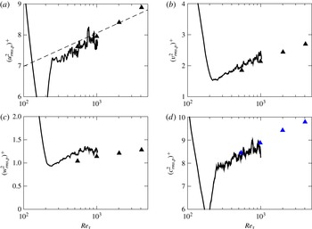
One of the strengths of the temporal approach is the opportunity to study the evolution of quantities with time, or equivalently, increasing Reynolds number. An example is shown in figure 17 where the peak of the variance is plotted for (a) streamwise, (b) spanwise and (c) wall-normal velocity for the
 $Re_{D}\approx 500$
(series B) case. Channel DNS data from Bernardini, Pirozzoli & Orlandi (Reference Bernardini, Pirozzoli and Orlandi2014) is also plotted for comparison, which is sourced from four separate simulations at specified Reynolds numbers (
 $Re_{{\it\tau}}=550,~999,~2022,~4079$
). Our data here has not been time-window averaged and the lines appear jagged, however as suggested by the relation given by Hutchins et al. (Reference Hutchins, Nickels, Marusic and Chong2009) for the streamwise variance peak, it is nonetheless possible to discern a logarithmic development in the value of the velocity variance peaks above
 $Re_{{\it\tau}}\approx 200$
. We find reasonable agreement with the data shown by Bernardini et al. (Reference Bernardini, Pirozzoli and Orlandi2014) for the lower
 $Re_{{\it\tau}}$
which we achieve, and consider this example to be a particularly compelling argument for the utility of the temporal approach. The increasing near-wall root-mean-squared peak is linked with the footprint of large-scale structures therefore it is here apparent that the temporal simulation can capture large-scale structures.
Evolution of the square of the peak of the variance versus
 $Re_{{\it\tau}}$
for (thick solid line)
 $Re_{D}\approx 500$
, series B: (a) streamwise velocity; – – –, relation
 $(3.1)$
from Hutchins et al. (Reference Hutchins, Nickels, Marusic and Chong2009) which for
 $l^{+}=0$
takes the form
 $(u_{rms,p}^{2})^{+}=1.0747\log _{10}Re_{{\it\tau}}+4.8371$
; (b) spanwise velocity; (c) wall-normal velocity (d) scalar; ▴ (black), Bernardini et al. (Reference Bernardini, Pirozzoli and Orlandi2014); ▴ (blue), Pirozzoli, Bernardini & Orlandi (Reference Pirozzoli, Bernardini and Orlandi2016).

5.2 Similarity solutions
To what extent is the similarity between the spatially and temporally developing turbulent boundary layers to be expected? We find that expressions for the skin friction coefficient such as (1.4) differ, but how does this difference manifest itself for large Reynolds numbers? Townsend (Reference Townsend1956) (§
 $10.4$
) details a similarity solution using classical scaling for the spatially developing turbulent boundary layer, as does Jones, Nickels & Marusic (Reference Jones, Nickels and Marusic2008), whereby similarity solutions to the Reynolds-averaged Navier–Stokes equations (1.3) are sought. Where they neglect the viscous term in the limit of infinite Reynolds number, we will also drop the difference in normal Reynolds stresses
 $\partial (\overline{u^{\prime 2}}-\overline{w^{\prime 2}})/\partial x$
to simplify the ensuing analysis. For a free-stream velocity of
 $U_{\infty }$
, the proposed solution therefore takes the form (where notation has been adjusted to match the present case):
 $$\begin{eqnarray}\displaystyle \frac{U_{\infty }-\overline{u}}{u_{{\it\tau}}(x)}=f({\it\eta}), & & \displaystyle\end{eqnarray}$$
 $$\begin{eqnarray}\displaystyle -\frac{\overline{w^{\prime }u^{\prime }}}{u_{{\it\tau}}^{2}(x)}=f_{rs}({\it\eta}), & & \displaystyle\end{eqnarray}$$
where
 ${\it\eta}=z/{\it\delta}(x)$
. After substitution into (1.3), this yields
 $$\begin{eqnarray}\underbrace{\frac{{\it\delta}U_{\infty }}{u_{{\it\tau}}^{2}}\frac{\text{d}u_{{\it\tau}}}{\text{d}x}}_{a_{1}}f-\underbrace{\frac{U_{\infty }}{u_{{\it\tau}}}\frac{\text{d}{\it\delta}}{\text{d}x}}_{a_{2}}{\it\eta}f^{\prime }-\underbrace{\frac{{\it\delta}}{u_{{\it\tau}}}\frac{\text{d}u_{{\it\tau}}}{\text{d}x}}_{a_{3}}(f^{2}-I_{1}f^{\prime })+\underbrace{\frac{\text{d}{\it\delta}}{\text{d}x}}_{a_{4}}I_{1}f^{\prime }+\underbrace{1}_{a_{5}}f_{rs}^{\prime }=0,\end{eqnarray}$$
where
 $I_{1}\equiv \int _{0}^{{\it\eta}}f({\it\eta}^{\prime })\,\text{d}{\it\eta}^{\prime }$
. As per the usual assumption in the classical method, the Reynolds stress velocity scale has been set to
 $u_{{\it\tau}}$
in writing the above, which results in
 $a_{5}=1$
, and the length scale has been set to
 ${\it\delta}$
. Jones et al. (Reference Jones, Nickels and Marusic2008) develop expressions for
 $a_{1}-a_{4}$
which are functions of
 $U_{\infty }^{+}$
only, and they consequently find that as
 $U_{\infty }^{+}\rightarrow \infty$
, the only coefficient that balances the term with coefficient
 $a_{5}$
is
 $a_{2}\rightarrow 1/C_{1}=1/\int _{0}^{\infty }f({\it\eta})\,\text{d}{\it\eta}$
, the other terms decaying to zero.
Akin to that shown above for the spatial boundary layer, we summarise below the similarity solution for the temporal boundary layer, and examine how solution coefficients behave for large Reynolds numbers compared to that of the spatially developing case. This follows the analysis of the Rayleigh problem given by Crow (Reference Crow1968).
Starting with the Reynolds-averaged Navier–Stokes equations for the temporal set-up (1.2) shown earlier, we now drop the viscous term as did Jones et al. (Reference Jones, Nickels and Marusic2008), and use a similarity solution of the form:
 $$\begin{eqnarray}\frac{\overline{u}}{u_{{\it\tau}}(X)}=g({\it\eta}),\end{eqnarray}$$
 $$\begin{eqnarray}\frac{\overline{w^{\prime }u^{\prime }}}{u_{{\it\tau}}^{2}(X)}=g_{rs}({\it\eta}),\end{eqnarray}$$
where
 ${\it\eta}=z/{\it\delta}(X)$
and
 $X=U_{w}t$
. We may rewrite (1.2) as
 $$\begin{eqnarray}\frac{{\it\delta}u_{{\it\tau}}^{\prime }}{u_{{\it\tau}}^{2}}(-g)+\frac{{\it\delta}^{\prime }}{u_{{\it\tau}}}(g^{\prime }{\it\eta})=g_{rs}^{\prime }.\end{eqnarray}$$
Putting
 $U_{w}^{+}=U_{w}/u_{{\it\tau}}$
, we may recast the problem as
 $$\begin{eqnarray}\underbrace{-{\it\delta}\frac{\text{d}U_{w}^{+}}{\text{d}X}}_{b_{1}}g-\underbrace{U_{w}^{+}\frac{\text{d}{\it\delta}}{\text{d}X}}_{b_{2}}{\it\eta}g^{\prime }+\underbrace{1}_{b_{3}}g_{rs}^{\prime }=0.\end{eqnarray}$$
We now seek to rewrite the coefficients on the left-hand side in terms of
 $U_{w}^{+}$
exclusively. Using (1.4) and (1.6) we arrive at:
 $$\begin{eqnarray}-{\it\delta}\frac{\text{d}U_{w}^{+}}{\text{d}X}+U_{w}^{+}\frac{\text{d}{\it\delta}}{\text{d}X}=\frac{1}{C_{1}},\end{eqnarray}$$
the constant
 $C_{1}$
having been defined by (1.7) for the present set-up. Furthermore, making use of the composite law of the wall/wake (1.5) at
 $z={\it\delta}$
(where
 $\overline{u}=0$
in our case) we can write:
 $$\begin{eqnarray}{\it\kappa}\frac{\text{d}U_{w}^{+}}{\text{d}X}=\frac{1}{{\it\delta}}\frac{\text{d}{\it\delta}}{\text{d}X}-\frac{1}{U_{w}^{+}}\frac{\text{d}U_{w}^{+}}{\text{d}X}.\end{eqnarray}$$
Having now two equations (5.8) and (5.9), we can solve for
 $\text{d}U_{w}^{+}/\text{d}X$
and
 $\text{d}{\it\delta}/\text{d}X$
, giving expressions that are only functions of
 $U_{w}^{+}$
:
 $$\begin{eqnarray}\frac{\text{d}U_{w}^{+}}{\text{d}X}=\frac{1}{C_{1}{\it\kappa}{\it\delta}U_{w}^{+}},\end{eqnarray}$$
 $$\begin{eqnarray}\frac{\text{d}{\it\delta}}{\text{d}X}=\frac{1+{\it\kappa}U_{w}^{+}}{C_{1}{\it\kappa}(U_{w}^{+})^{2}}.\end{eqnarray}$$
For large
 $U_{w}^{+}$
, the only coefficient that is not asymptotically zero is
 $$\begin{eqnarray}b_{2}=U_{w}^{+}\frac{\text{d}{\it\delta}}{\text{d}X}\longrightarrow \frac{1}{C_{1}},\end{eqnarray}$$
which is the same result as in Jones et al. (Reference Jones, Nickels and Marusic2008) for the spatially developing case.
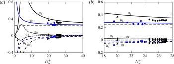
Plotting these coefficients as a function of
 $U_{w}^{+}$
or
 $U_{\infty }^{+}$
, as shown in figure 18(a), along with those given by Jones et al. (Reference Jones, Nickels and Marusic2008), should allow us to discern at which
 $U_{w}^{+}$
or
 $U_{\infty }^{+}$
the similarity solution of the temporal turbulent boundary layer approaches that of the spatially developing turbulent boundary layer, that is, at which point those terms that are different decay sufficiently. The constants
 ${\it\kappa}$
,
 $C_{1}$
and
 $C_{2}$
from table 2 (Present) are used to plot the coefficients for both the spatial and temporal formulations. Along with these curves issuing from the respective models, we also plot the value of these coefficients calculated using DNS data for both the spatially developing simulations of Skote (Reference Skote2001) and Sillero, Jiménez & Moser (Reference Sillero, Jiménez and Moser2013), along with the current temporal case. A zoomed-in view is presented in figure 18(b). Gradients are calculated over intervals of
 ${\rm\Delta}Re_{{\it\tau}}\approx 100$
for each dataset.
The analysis for the temporal case is well supported by the present data. The temporal simulations clearly approach the asymptote quicker (at a smaller
 $U_{w}^{+}$
) than the spatial simulations. For ‘surviving’ coefficient
 $a_{2}$
in the spatial case, both spatial datasets yield values closer to the asymptote, and therefore closer to the temporal case, than that given by the analytical curve. Our temporal data matches the analytical curve well for both coefficients
 $b_{1}$
and
 $b_{2}$
since periodic boundary conditions in the temporal simulation from the beginning force the parallel flow assumed in the similarity solution formulation. In contrast, the parallel-flow condition is only asymptotic in the formulation of Jones et al. (Reference Jones, Nickels and Marusic2008) for the spatially developing turbulent boundary layer. Yet the numerical values for the spatial simulations point to their being closer to the asymptotic state for a given
 $U_{\infty }^{+}$
than that expected by the analysis. The difference between the spatial and temporal cases is therefore not as significant as suggested by the analytical expressions for the coefficients of the similarity solution over the range of
 $U_{w}^{+}$
covered by the present simulations. This illustrates why the outer-layer wake of the two cases matches convincingly as is shown in figure 16.
Therefore we find that both the analysis and the data show that at large Reynolds numbers, the dominant balances in the outer layer for the spatial and temporal cases are equal:
 $$\begin{eqnarray}-\!\underbrace{U_{\infty }^{+}\frac{\text{d}{\it\delta}}{\text{d}x}}_{a_{2}}{\it\eta}f^{\prime }+f_{rs}^{\prime }=0,\quad -\!\underbrace{U_{w}^{+}\frac{\text{d}{\it\delta}}{\text{d}X}}_{b_{2}}{\it\eta}g^{\prime }+g_{rs}^{\prime }=0\end{eqnarray}$$
and we have here shown that the remaining coefficients
 $a_{2}$
and
 $b_{2}$
both tend to an asymptotic value of
 $1/C_{1}$
. In this sense, the asymptotic spatial boundary layer is in fact the temporal boundary layer.
Coefficients of the similarity solutions for both the temporal and spatial turbulent boundary layers as a function of
 $U_{w}^{+}$
(or
 $U_{\infty }^{+}$
for the spatial case): (a) coefficients as labelled in (5.3) and (5.7); (b) zoomed-in view; – – –,
 $1/C_{1}$
; data from spatially developing simulations: ▴, zero-pressure-gradient case of Skote (Reference Skote2001); ● (black),
 $BL_{6600}$
case of Sillero et al. (Reference Sillero, Jiménez and Moser2013); ● (blue), current temporal simulation,
 $Re_{D}\approx 500$
, series B case.

6 Passive scalar
6.1 Stanton number
In addition to the incompressible Navier–Stokes equations, the passive scalar equation was solved:
 $$\begin{eqnarray}\frac{\partial c}{\partial t}+u_{j}\frac{\partial c}{\partial x_{j}}=\mathscr{D}\frac{\partial ^{2}c}{\partial x_{j}^{2}},\end{eqnarray}$$
where
 $\mathscr{D}$
is the diffusivity of the scalar (not to be confused with trip height
 $D$
) for a Schmidt number
 $Sc={\it\nu}/\mathscr{D}=1.0$
. The Stanton number
 $St$
, representing the mass transfer coefficient, is a quantity of interest, being the scalar counterpart to the skin friction coefficient
 $C_{f}$
. It is given by
 $$\begin{eqnarray}St=\frac{j_{w}}{(U_{w}-U_{\infty })(C_{w}-C_{\infty })}=\frac{c_{{\it\tau}}u_{{\it\tau}}}{U_{w}C_{w}}=\frac{1}{U_{w}^{+}C_{w}^{+}},\end{eqnarray}$$
where
 $j_{w}=-\left.\mathscr{D}~\partial \overline{c}/\partial z\right|_{w}$
is the wall scalar flux, and
 $U_{\infty }=C_{\infty }=0$
as previously stated, with
 $c_{{\it\tau}}$
given by:
 $$\begin{eqnarray}c_{{\it\tau}}=\frac{\left.-\mathscr{D}{\displaystyle \frac{\partial \overline{c}}{\partial z}}\right|_{w}}{u_{{\it\tau}}}.\end{eqnarray}$$
Similar to that applied to the streamwise velocity, a composite average profile is assumed for the scalar:
 $$\begin{eqnarray}\frac{C_{w}-\overline{c}}{c_{{\it\tau}}}=\frac{1}{{\it\kappa}_{c}}\log \left(\frac{zu_{{\it\tau}}}{{\it\nu}}\right)+A_{c}(Sc)+\frac{{\it\Pi}_{c}}{{\it\kappa}_{c}}w_{c}\left(\frac{z}{{\it\delta}_{c}}\right),\end{eqnarray}$$
with counterpart constants to that for the streamwise velocity. Here
 ${\it\delta}_{c}$
is the scalar counterpart to the 99 % boundary layer thickness. Writing (6.4) at
 $z={\it\delta}_{c}$
where
 $\overline{c}=0$
, using (6.2), and expressing
 $U_{w}^{+}=(2/C_{f})^{1/2}$
we can write:
 $$\begin{eqnarray}St=\frac{(C_{f}/2)^{1/2}}{{\displaystyle \frac{1}{{\it\kappa}_{c}}}\log [Re_{{\it\delta}}(C_{f})^{1/2}]+(\log ({\it\delta}_{c}/{\it\delta})-{\displaystyle \frac{1}{2}}\log (2))/{\it\kappa}_{c}+{\it\phi}_{c}(1,Sc)},\end{eqnarray}$$
where
 ${\it\phi}_{c}(1,Sc)=A_{c}(Sc)+({\it\Pi}_{c}/{\it\kappa}_{c})w_{c}(1)$
. This is a very similar approach to that of Yaglom (Reference Yaglom1979), whose expression for
 $St$
took the form:
 $$\begin{eqnarray}St=\frac{(C_{f}/2)^{1/2}}{{\it\alpha}\log [Re_{{\it\delta}}(C_{f})^{1/2}]+{\it\beta}_{2}(Pr)},\end{eqnarray}$$
where
 ${\it\alpha}$
is a universal constant and
 ${\it\beta}_{2}$
depends on
 $Pr$
.
 $Re_{{\it\delta}}$
is also given as function of
 $C_{f}$
in Kader & Yaglom (Reference Kader and Yaglom1972). The principal difference between our present formulation and that of Yaglom (Reference Yaglom1979) is the use and selection of constants.
In order to plot the Stanton number against Reynolds numbers for which we developed expressions that were functions of
 $U_{w}^{+}$
only, we seek to develop an expression for
 $St$
that is also only a function of
 $U_{w}^{+}$
. We therefore make the approximation here that
 ${\it\delta}_{c}\approx {\it\delta}$
although it appears to be increasingly inaccurate with increasing Reynolds number (
 $({\it\delta}-{\it\delta}_{c})/{\it\delta}_{c}\approx 0.3$
at
 $Re_{{\it\tau}}=1000$
for the
 $Re_{D}\approx 500$
, series B, case). Nevertheless, using (1.9):
 $$\begin{eqnarray}Re_{{\it\delta}}\equiv U_{w}{\it\delta}/{\it\nu}=U_{w}^{+}\exp ({\it\kappa}[U_{w}^{+}-{\it\phi}(1)]),\end{eqnarray}$$
we are able to write
 $$\begin{eqnarray}St=\frac{1}{U_{w}^{+}\left({\displaystyle \frac{1}{{\it\kappa}_{c}}}({\it\kappa}[U_{w}^{+}-{\it\phi}(1)])+{\it\phi}_{c}(1)\right)}.\end{eqnarray}$$
It is necessary to establish values of the constants in (6.8) so that it may be plotted as a function of
 $U_{w}^{+}$
. Using the definition of the scalar displacement thickness combined with (6.4) we arrive at:
 $$\begin{eqnarray}\frac{{\it\delta}_{c}^{\ast }}{{\it\delta}_{c}}=C_{1,c}\frac{c_{{\it\tau}}}{C_{w}}=\frac{C_{1,c}}{C_{w}^{+}},\end{eqnarray}$$
where the scalar displacement thickness is defined as
 ${\it\delta}_{c}^{\ast }\equiv \int _{0}^{\infty }(\overline{c}/C_{w})\,\text{d}z$
, and
 $C_{1,c}$
is a constant. A fit of
 ${\it\kappa}_{c}=0.42$
and
 $A_{c}=5.2$
is found for the logarithmic region of the mean scalar profile, compared to
 ${\it\kappa}=0.384$
and
 $A=4.173$
for the streamwise velocity. As for the streamwise velocity, plotting
 $C_{w}^{+}{\it\delta}_{c}^{\ast }/{\it\delta}_{c}$
with time shows that
 $C_{1,c}$
stabilises to a value of
 $C_{1,c}\approx 3.4$
(cf.
 $C_{1}=4.05$
) for the
 $Re_{D}\approx 500$
(series B) case.
The current data reveals that the wake of the scalar is not a simple rescaling of that of the streamwise velocity, with normalising conditions
 $w_{c}(0)=0$
and
 $w_{c}(1)=2$
imposed. The shape of the scalar wake function
 $w_{c}(z/{\it\delta}_{c})$
may be generalised by allowing the normalising condition
 $\int _{0}^{2}(z/{\it\delta}_{c})(w_{c})\,\text{d}w_{c}={\it\gamma}$
, where
 ${\it\gamma}$
is a constant, noting
 ${\it\gamma}=1$
for the wake of the streamwise velocity
 $w(z/{\it\delta})$
. The constant analogous to
 $C_{1}=(1+{\it\Pi})/{\it\kappa}$
for the velocity then becomes
 $C_{1,c}=(1+{\it\gamma}{\it\Pi}_{c})/{\it\kappa}_{c}$
for the scalar given this new normalising condition. Fitting a curve
 $(-1/{\it\kappa}_{c})\log (z/{\it\delta}_{c})+w_{c}(1){\it\Pi}_{c}/{\it\kappa}_{c}$
to the data
 $\overline{c}/c_{{\it\tau}}$
(defect form) allows us to estimate
 ${\it\Pi}_{c}\approx 0.30$
. The expression for
 $C_{1,c}$
then gives
 ${\it\gamma}\approx 1.4$
. Since the normalising condition on the wake profile is in fact the compliment integral, this suggests the normalised area of the wake is
 $2-{\it\gamma}\approx 0.6$
, which has been verified by integrating the wake from the mean scalar profile. Therefore we are able to estimate
 ${\it\phi}_{c}(1,Sc)=A_{c}(Sc)+2{\it\Pi}_{c}/{\it\kappa}_{c}\approx 6.6$
. It is now possible to compare the constants in our (6.5) to that of (6.6). In the present case,
 $1/{\it\kappa}_{c}\approx 2.4$
, whereas Yaglom (Reference Yaglom1979) gives
 ${\it\alpha}\approx 2.12$
. Assuming that
 ${\it\delta}_{c}/{\it\delta}\approx 1$
, we can evaluate
 $(\log ({\it\delta}_{c}/{\it\delta})-\log (2)/2)/{\it\kappa}_{c}+{\it\phi}_{c}(1,Sc)\approx 5.8$
. The analogous constant from Yaglom (Reference Yaglom1979) is
 ${\it\beta}_{2}={\it\beta}(Pr)+{\it\beta}_{1}-{\it\alpha}(\log 2)/2$
. For
 $Pr=1$
,
 ${\it\beta}\approx 6.8$
according to relation (17) in the work. Since Yaglom (Reference Yaglom1979) does not cite a conclusive value for the constant
 ${\it\beta}_{1}$
, we will here take it to be
 $w_{c}(1){\it\Pi}_{c}/{\it\kappa}_{c}\approx 1.4$
to which it corresponds in the present case. We can then calculate
 ${\it\beta}_{2}\approx 7.5$
. The constants thus settled, we find the denominators of (6.5) and (6.6) differ by around 1 % at
 $Re_{{\it\tau}}\approx 1000$
for the
 $Re_{D}\approx 500$
(series B) case.
6.2 Scalar results
In a manner parallel to figure 5(b) where
 $C_{f}=2/(U_{w}^{+})^{2}$
was plotted, figure 19(a) shows the development of the mass transfer coefficient or Stanton number
 $St$
for the
 $Re_{D}\approx 500$
(series B) case, given by (6.2). We also plot the relation (6.8) against (1.14). For a given
 $Re_{{\it\theta}}$
,
 $U_{w}^{+}$
can be obtained from (1.14).
 $St$
can then be calculated by (6.8). In figure 19(a) it is plotted for a range of
 $U_{w}^{+}$
as was done in figure 5. We find a reasonably good fit with the data, although the curve deviates increasingly at high
 $Re_{{\it\theta}}$
, the difference approaching
 $6\,\%$
for
 $Re_{{\it\theta}}\approx 3000$
. One possible explanation is the approximation
 ${\it\delta}_{c}\approx {\it\delta}$
, which, as was noted above, gets worse with growing Reynolds number. However we emphasise the appeal of this curve given that it is a simple expression allowing
 $St$
to be plotted as a function of
 $U_{w}^{+}$
only. In addition, the relation of Kays & Crawford (Reference Kays and Crawford1993) is plotted using the data series for
 $Re_{{\it\theta}}$
:
 $$\begin{eqnarray}St=0.0125~Pr^{-2/5}Re_{{\it\theta}}^{-1/4},\quad Pr>0.5,\end{eqnarray}$$
where
 $Pr=Sc$
here, and again we find reasonable agreement with our data. However such a power-law formulation is not expected to fit the data over the whole range of Reynolds numbers, and indeed we find it deviates from the present simulation at higher
 $Re_{{\it\theta}}$
.
The mean profile for the scalar
 $c$
is plotted for this same case in figure 19(b) at two different
 $Re_{{\it\theta}}$
, with data from the spatially developing boundary layer DNS of Wu & Moin (Reference Wu and Moin2010) shown for reference. With this spatial data we again find excellent agreement. Note the similarity between these scalar mean profiles and those for the streamwise velocity in figure 8. We are again able to identify a viscous sublayer and a nascent logarithmic region as we were able to for the streamwise velocity. As observed by Pirozzoli et al. (Reference Pirozzoli, Bernardini and Orlandi2016), the wake strength is here greater in the velocity field than in the scalar field.
(a) Development of Stanton number with
 $Re_{{\it\theta}}$
: thick solid line,
 $Re_{D}\approx 500$
, series B; thin solid line,
 $St(U_{w}^{+})$
(6.8) versus
 $Re_{{\it\theta}}(U_{w}^{+})$
(1.14);
 $\cdots \cdots$
, correlation of Kays & Crawford (Reference Kays and Crawford1993); (b) Mean scalar profile for two different
 $Re_{{\it\theta}}$
: – – –,
 $C_{w}^{+}-\overline{c}^{+}=Sc~z^{+}$
and
 $C_{w}^{+}-\overline{c}^{+}=(1/{\it\kappa}_{c})\log z^{+}+A_{c}(Sc)$
; ●, spatially developing simulation of Wu & Moin (Reference Wu and Moin2010).

Second-order statistics for the scalar are plotted in figure 20(a–c) for this same case, again at two different
 $Re_{{\it\theta}}$
. We find very good agreement for our scalar statistics with those of Wu & Moin (Reference Wu and Moin2010), although our peak in scalar fluctuations is slightly less, as Pirozzoli et al. (Reference Pirozzoli, Bernardini and Orlandi2016) also observe at
 $Pr=1$
. Comparing the profiles for
 $c_{rms}^{+}$
in 20(a) and
 $u_{rms}^{+}$
in figure 9(a), we find the profiles to be very similar, and note that the peak for both quantities occurs at
 $z^{+}\approx 13$
. We also note the striking similarity between profiles for
 $\overline{w^{\prime }u^{\prime }}^{+}$
in figure 9(c) and those of
 $\overline{w^{\prime }c^{\prime }}/u_{{\it\tau}}c_{{\it\tau}}$
in figure 20(c), suggesting that scalar
 $c$
is transported in much the same way as streamwise momentum i.e. Reynolds analogy.
Scalar second-order statistics at two different
 $Re_{{\it\theta}}$
: ——,
 $Re_{D}\approx 500$
, series B; ●, spatially developing simulation of Wu & Moin (Reference Wu and Moin2010). Note that in (b) and (c) the data from Wu & Moin (Reference Wu and Moin2010) is actually
 $-\overline{u^{\prime }c^{\prime }}^{+}$
and
 $-\overline{w^{\prime }c^{\prime }}^{+}$
respectively – the sign is reversed here for the present temporal configuration. (d) Turbulent Schmidt number as a function of
 $z^{+}$
at
 $Re_{{\it\theta}}=800~(Re_{{\it\tau}}\approx 320)$
. Data from spatially developing simulations: ●, Li et al. (Reference Li, Schlatter, Brandt and Henningson2009),
 $Re_{{\it\theta}}=800$
,
 $Pr=0.71$
; ○, Kim & Moin (Reference Kim and Moin1987),
 $Re_{{\it\tau}}=180$
,
 $Pr=0.71$
.

The turbulent Schmidt number is a parameter of interest for scalar transfer and is plotted in figure 20(d). It is defined as:
 $$\begin{eqnarray}Sc_{t}=\frac{{\it\nu}_{t}}{\mathscr{D}_{t}},\end{eqnarray}$$
where
 ${\it\nu}_{t}=\overline{u^{\prime }w^{\prime }}/\partial \overline{u}/\partial z$
is the turbulent eddy viscosity, and
 $\mathscr{D}_{t}=\overline{w^{\prime }c^{\prime }}/\partial \overline{c}/\partial z$
is the eddy diffusivity. We find good agreement for our
 $Re_{D}\approx 500$
(series B) case with the data of Kim & Moin (Reference Kim and Moin1987) and Li et al. (Reference Li, Schlatter, Brandt and Henningson2009), even though in their case
 $Pr=0.71$
(cf. our Schmidt number
 $Sc=1.0$
). The reader may note the use of three different datasets. For figures 20(a–c), we have compared against the data of Wu & Moin (Reference Wu and Moin2010) since data is available for two
 $Re_{{\it\theta}}$
within the span of our simulation such that we may replicate the two-panel format of figures 9 and 11, among others, allowing us to demonstrate how our simulation compares against that of a spatial simulation throughout. This dataset was also chosen since Wu & Moin (Reference Wu and Moin2010) use
 $Pr=1$
(compared to the present
 $Sc=1$
). The data for Li et al. (Reference Li, Schlatter, Brandt and Henningson2009) only reaches
 $Re_{{\it\theta}}\approx 800$
with the closest Prandtl number to ours being
 $Pr=0.71$
. However, for the turbulent Prandtl number of figure 20(d), comparison is against the results of Kong, Choi & Lee (Reference Kong, Choi and Lee2000) and Li et al. (Reference Li, Schlatter, Brandt and Henningson2009), since Wu & Moin (Reference Wu and Moin2010) report a turbulent Prandtl number well in excess of other studies.
We have also shown in figure 17(d) how the peak scalar variance evolves with time and find good agreement with the data of Pirozzoli et al. (Reference Pirozzoli, Bernardini and Orlandi2016) for our more limited range of
 $Re_{{\it\tau}}$
.
7 Conclusions
We have investigated the incompressible temporally developing turbulent boundary layer and compared it to its spatially developing counterpart. The two flows are similar in many respects, including turbulent skin friction development and mean profiles (figures 5 and 8) and turbulent profiles (figure 9). As expected, the effect of initial conditions cannot be neglected. Presently, this aspect of the simulation is investigated using an inflectional
 $\tanh$
profile that models the shear-layer wake of a wall-mounted trip, characterising it with one length dimension only, trip height
 $D$
. For the small trip of
 $Re_{D}\approx 250$
, the boundary layer remains laminar, but for
 $Re_{D}\approx 500$
the boundary layer transitions and quickly assumes a natural or undisturbed development at the smallest
 $Re_{{\it\theta}}$
. Alternatively, an initial trip of
 $Re_{D}\approx 1000$
results in natural evolution at the earliest possible time, equivalently at the smallest
 $Re_{X=U_{w}t}$
.
Flow statistics such as mean streamwise velocity, variance as well as higher-order streamwise skewness and flatness, reveal the extent to which the trip Reynolds number affects the flow. At
 $Re_{{\it\theta}}=1100$
, the cases with the two smaller trips
 $Re_{D}\approx 500$
and
 $Re_{D}\approx 1000$
already collapse, however profiles of the two larger trip cases
 $Re_{D}\approx 1500$
and
 $Re_{D}\approx 2000$
differ. Yet, at the later
 $Re_{{\it\theta}}=1968$
, all cases have largely collapsed, with some exceptions regarding
 $Re_{D}\approx 2000$
(i.e.
 $w_{rms}^{+}$
and
 $p_{rms}^{+}$
). A contour map of
 $u_{rms}^{+}$
allows us to quantify the
 $Re_{{\it\theta}}$
for which we achieve collapse at the different
 $Re_{D}$
for inner and outer scales, and we find the required Reynolds number increases linearly with
 $Re_{D}$
. These contours also allow us to conclude that a value of
 ${\it\theta}/D\approx 1$
is required to ensure a flow that is unencumbered by its starting
 $Re_{D}$
.
One-dimensional energy spectra of the case
 $Re_{D}\approx 500$
at
 $Re_{{\it\tau}}=590$
for two different computational box sizes (
 $L_{x}/{\it\delta}\approx 6.7$
and
 $L_{x}/{\it\delta}\approx 11.2$
) allow us to ascertain the impact of domain size. It appears that our smaller simulation may be restricting some of the larger scales in the streamwise direction whereas the spanwise scales appear rather less impacted by our choice of box size. However, the spectra do not differ greatly therefore we are able to conclude that our smaller domain adequately reproduces the main dynamical features of the flow up to the
 $Re_{{\it\tau}}=590$
for which it was planned.
Both the velocity and scalar statistics are found to agree very well with spatial data from both experimental and numerical studies in the literature. Additionally, it is shown analytically that the spatial and temporal turbulent boundary layers evolve similarly by comparing their respective similarity solutions. The present results suggest that the temporally developing boundary layer is a good model for the spatially developing boundary layer. The temporal boundary layer is a viable tool if the goal is to obtain moderately converged one-point statistics; the extent to which two-point statistics agree will have to await comparison between spatial boundary layer and temporal boundary layer spectra.
Aside from representing an interesting flow worthy of study for its own sake, we believe that the temporal set-up is an under-exploited tool that may prove useful for understanding turbulent boundary layers in general. Important differences between the spatial and temporal boundary layers may aid in clarifying the origins of certain phenomena. For example, the present study suggests that non-parallel effects are perhaps not that important after all, at least for the quantities that have been considered. Our results also demonstrate that statistics including the mean streamwise velocity, various variances, streamwise skewness and flatness are not contingent on spatial growth. The increasing near-wall root-mean-squared velocity peaks thought to be linked to the footprint of large-scale structures are also reproduced by the idealised temporal set-up. That is, the temporal boundary layer appears to possess similar statistical signatures of large-scale motions to that of the spatial boundary layer. Its relative ease of set-up and potential cost saving with respect to the long-domain studies of spatially developing turbulent boundary layers make it an attractive method by which to study various manipulations of the turbulent boundary layer, beyond the simplified tripping mechanism studied here.
Acknowledgements
M.K. gratefully acknowledges funding provided by the Australian Research Council. This research was partly undertaken on the NCI National Facility in Canberra, Australia, which is supported by the Australian Government. This work was also supported by resources provided by the Pawsey Supercomputing Centre with funding from the Australian Government and the Government of Western Australia.
Appendix. Time-window averaging
This temporal computational set-up yields data resolved in time. Where spatially developing data is generally ensemble-averaged as is done for experimental data, such a temporal simulation does not present that opportunity, unless of course the simulations are repeated many times at commensurate cost. ‘Progress’ quantities, such as those shown in figures 5 and 6, are plots of the instantaneous values to reflect this. However, profiles of statistics at specific points in time (i.e. specific Reynolds numbers) appear unconverged and jagged. In an effort to smooth statistics, windows of
 ${\it\alpha}{\it\delta}/u_{{\it\tau}}$
, where
 ${\it\alpha}$
is a constant, were used to limit the effect of a single eddy on profiles of various quantities presented. Thus setting
 ${\it\alpha}$
fixes the width (in time) of the window centred at the time where we want to plot statistics. This ‘smoothing’ effect is most exaggerated for the smaller domain at high-order statistics, since a larger domain is less impacted by an individual structure for a given Reynolds number.
Ensemble versus time-window averaging on statistics for
 $Re_{D}\approx 500$
, series A (small domain) for second-order streamwise root-mean-squared velocity: (a) profiles from three different realisations at a single time at
 $Re_{{\it\theta}}=1968$
; (b) ensemble-averaged result; (c) skin friction profile as a function of
 $Re_{X}$
showing upper and lower bounds of
 $C_{f}$
for
 ${\it\alpha}=0.5$
; (d) effect of window averaging at
 $Re_{{\it\theta}}=1968$
for
 ${\it\alpha}=0.5$
;
 $\unicode[STIX]{x1D664}$
, DNS of Jiménez et al. (Reference Jiménez, Hoyas, Simens and Mizuno2010) at
 $Re_{{\it\theta}}=1968$
.

Figure 21 shows the impact of ensemble averaging with multiple realisations versus time-window averaging for the second-order streamwise root-mean-squared velocity for the
 $Re_{D}\approx 500$
, series A (small domain) case. Figure 21(a) shows three realisations, each initiated with a different random noise, of this case at a single time. The three profiles are then averaged to produce 21(b). The time-window averaging method used in the present work is presented directly below that subfigure. A maximum of
 ${\it\alpha}=0.5$
was used for statistics presented herein, and for this time window, figure 21(c) shows that the effect on
 $C_{f}$
is of the order of a few percent. The ‘upper’ and ‘lower’ bounds of
 $C_{f}$
at any point in time when using such averaging are in fact not always above and below the original curve – this is only the case if the curve is monotonically increasing or decreasing. For example, at the peak of
 $C_{f}$
, stepping both forward and backward in time about the central time yields a set of values for averaging which are all actually smaller than the value at the time when the peak occurred, since there is no value greater than it. Figure 21(d) demonstrates that the main effect of the window averaging is to smooth jagged curves, without compromising the validity of the statistics, suggested by the agreement with the DNS of Jiménez et al. (Reference Jiménez, Hoyas, Simens and Mizuno2010) for a matched
 $Re_{{\it\theta}}=1968$
. We therefore find that for the modest convergence goals of this study, there appears to be little difference between ensemble and window averaging.
As we use time-window averaging for the temporal problem, Jiménez et al. (Reference Jiménez, Hoyas, Simens and Mizuno2010) make use of spatial window averaging for the spatial problem in addition to time averaging. Statistics at a nominal
 $Re_{{\it\theta}}=1968$
, in addition to being averaged over time, are averaged in the spanwise direction over the interval
 $(Re_{{\it\theta}_{0}},Re_{{\it\theta}_{1}})=(1938.2,1996.5)$
(range from their online database) in order to reduce statistical noise. In our case, data presented at
 $Re_{{\it\theta}}=1968$
for the
 $Re_{D}\approx 500$
, big box case, which is compared with spatial DNS in § 5, is averaged over a time window
 ${\it\alpha}{\it\delta}/u_{{\it\tau}}$
with
 ${\it\alpha}=0.5$
, representing averaging over the interval
 $(Re_{{\it\theta}_{0}},Re_{{\it\theta}_{1}})=(1831.7,2105.3)$
. A smaller window with
 ${\it\alpha}=0.1$
would result in a smaller range
 $(Re_{{\it\theta}_{0}},Re_{{\it\theta}_{1}})=(1941.1,1996.4)$
, very similar to that of Jiménez et al. (Reference Jiménez, Hoyas, Simens and Mizuno2010). However, the impact upon statistics of changing window size is small. The largest difference is found for higher-order statistics. For example, for fourth-order streamwise flatness,
 ${\it\alpha}=0.5$
gives a mean absolute difference from the data of Schlatter & Örlü (Reference Schlatter and Örlü2010) of
 $2.7\,\%$
up to
 $z^{+}=605$
. For the same range of
 $z^{+}$
, a smaller
 ${\it\alpha}=0.1$
gives a mean absolute difference of
 $3.7\,\%$
. We feel that the smoother statistics, that are closer to spatial DNS data, warrant the use of the larger time window, however we also point out here that the difference would be small had we used a smaller
 ${\it\alpha}$
.