2. Data sources and summary statistics

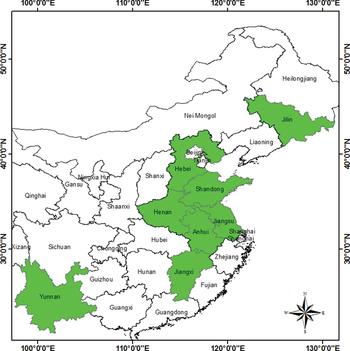
The data for agricultural production and household characteristics were collected from a large-scale household-level survey conducted in rural China in late 2012 and early 2013. Funding was available for the field survey in eight of the 34 provinces and regions of China (see figure 1). The survey was dependent on funding from several separate projects supporting research in specific provinces or regions, so it was conducted only in those provinces supported by these projects. Specifically, the survey in the provinces of Hebei, Henan, Anhui, Shandong, and Jiangsu was mainly supported by funding from the Ministry of Science and Technology in China, the survey in the provinces of Jiangxi and Yunnan was mainly supported by funding from the Australian Centre for International Agricultural Research, and the survey in Jilin province was mainly supported by the National Natural Sciences Foundation in China.

Figure 1.

Sample provinces of the survey in China.

Even though which provinces were included in the survey depended on funding availability, the eight sample provinces approximately represent the various agricultural systems in China. Specifically, the Jilin province represents the monoculture agricultural system in cold areas of China; Hebei, Henan, Anhui, Shandong, and Jiangsu represent the rotation agricultural system in China's temperate climate zone; the Jiangxi province represents rice production in southern China; and the Yunnan province represents agricultural production in the plateau climate zone. In addition, these eight sample provinces are important in Chinese agriculture. For example, they produced about 47 per cent of the total agricultural output in China each year; the other 53 per cent is produced by the remaining 26 provinces and regions in China.

Thirty-one sample counties were selected from the eight sample provinces. We selected three sample counties from each of seven sample provinces, but we selected 10 sample counties from Jiangxi because extra funding was available for this province. Within each sample province we divided all the counties into three groups (10 groups for Jiangxi) based on the condition of the agricultural production infrastructure and randomly selected one county from each group.

We selected the townships and villages before interviewing the actual households. Within each of the 31 selected counties, we divided all the townships into three groups based on the condition of the agricultural production infrastructure and randomly selected one township from each group. We used the same approach to select three villages from each township. Finally, we randomly selected 10 households for face-to-face interviews in each sampled village. We identified a total of 2,790 households in the eight provinces. After dropping the households with missing data for agricultural output, input, or household characteristics, the final sample used in the analysis comprised 2,733 households.

The farmlands in the survey are mainly used for crops and orchards.Footnote ⁴ The crop production and orchard data were collected separately. For land used for crop production, only the two larger plots were investigated if the household managed more than two plots. This sample selection rule helped to reduce measurement error because, in our data set, each household managed 7.6 plots on average and some plots were quite small. Collecting data from small plots might incur large measurement errors because, according to our experience, it is harder for farmers to precisely recall unit land inputs and outputs for a small plot. There is no major concern about the representativeness of the sample plots selected because, on average, the larger two plots took up 86.3 per cent of the cropland area managed by each farmer. For orchards, the data were collected for all orchards managed because each household usually managed only one or two orchards.

Household-level agricultural profits per hectare were collected for two years from 2010 to 2012.Footnote ⁵ According to the survey, farmers usually plant multiple crops in sequence in a plot within a year. The main growing season is usually used for staple crops, such as rice, wheat, and maize, while other seasons are used for minor crops, such as oilseed rape, beans, and vegetables. The profits per hectare were constructed as revenue minus cost. The revenues were the market value of all the products harvested in a year, and the costs were the total production expenditure in a year. The costs included only expenses for seed, fertilizers, pesticides, labor, and machinery.Footnote ⁶ Finally, the profits per hectare were translated into US dollars (USD) using China's rural Consumer Price Indices (CPI) and the exchange rate between RMB and USD as of 2010. In the following econometric analyses, we mainly used crop profits per hectare as the dependent variable. As a robustness check, we also provide analyses using the weighted average of profits per hectare from cropland and orchards as the dependent variable.

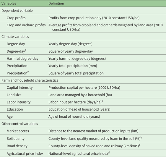
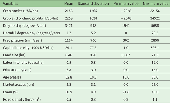
Detailed farm and household characteristics with the potential to affect agricultural profits and adaptive capacity were also collected in the survey. As defined in table 1, these characteristics include the capital intensity, labor intensity, and farmland size of the household; education level and age of the head of household; and market access. County-level agricultural land quality and road density were also included as control variables. County-level land quality was measured as the percentage of loam in the soil, while county-level road density was measured as the number of kilometers of paved road and railway within a county divided by the total area of the county. The summary statistics of the data are provided in table 2.

Table 1.

Definition of variables

^a The labor intensity is measured by the total working days per hectare per year. Since there are usually multiple growing seasons within a year, the labor inputs are the sum across growing seasons within a year.

^b Loam is a standard indicator of soil quality. Loam is considered ideal for agricultural uses because it retains nutrients and water, while still allowing excess water to drain away. The data come from Resources and Environment Data Centre of Chinese Academy of Sciences (http://www.resdc.cn/).

^c The road density is calculated by the authors from a shapefile of 1:100,000 scale road information map for the year 2008 in China. Road density is measured as the kilometers of paved road and railway within a county divided by the total area of the county.

^d The agricultural price index measures the prices received by farmers for agricultural goods and services. The data is derived from National Bureau of Statistics of China (http://www.stats.gov.cn).

Table 2.

Summary statistics of variables

Note: The definitions of the variables are provided in Table 1.

The county-level daily mean temperature and precipitation data were derived from the China Meteorological Data Sharing Service System (http://cdc.nmic.cn). This data set provides real data for each of the 677 meteorological stations throughout China and offers the most detailed and reliable climate data set in China. At least one meteorological station is sited in 22 of the 31 sample counties. For those counties with more than one meteorological station, county-level climate data was derived from the weather station that was the closest to the county centroid of each county. For the nine sample counties in which meteorological stations were not available, we instead used climate data from the nearest meteorological station.Footnote ⁷

Daily mean temperature and precipitation were used to construct values for county-level yearly degree-days (DD), yearly harmful degree-days (HDD), and yearly total precipitation (TP).Footnote ⁸ DD measures cumulative exposure to temperatures of between 8 and 32^°C during the year. For example, a day with a mean temperature below 8^°C contributes zero DDs, between 8 and 32^°C contributes the difference between the mean and 8^°C, and above 32^°C contributes 24 DDs. DD is the sum of daily measures across the calendar year. HDD captures the possible damage of extreme heat that exceeds this threshold. We follow previous studies such as Guiteras (Reference Guiteras2009) to calculate HDD by assigning each day with mean temperature above 34^°C the difference between that day's mean temperature and 34^°C, and then sum up the daily measures across the calendar year to get the yearly HDD. TP is the total precipitation in mm during the calendar year. For the robustness test in the econometric analysis, we also calculated the growing season degree-day and growing season total precipitation. We followed the literature in defining growing season to be from March to October.

Finally, to predict climate change impacts, we collected the latest climate change projections that were developed for the Fifth Assessment Report of the Intergovernmental Panel on Climate Change (IPCC). The climate projections from 21 modeling centers and two Representative Concentration Pathway (RCP) scenarios, namely RCP4.5 and RCP8.5, which represent the medium and highest scenarios, respectively, were downloaded from the NASA Earth Exchange Global Daily Downscaled Projections (NEX-GDDP) data set (https://cds.nccs.nasa.gov/nex-gddp). Each model provides daily minimum temperature, maximum temperature, and precipitation under each scenario for the period from 2006 to 2100, with a spatial resolution of 0.25 degrees×0.25 degrees (about 25 km×25 km). Each model also provides simulated historical daily data from 1950 to 2005 for the same spatial resolution.

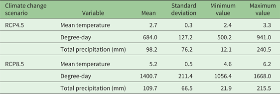
The climate change predictions were calculated as the difference between the 1976–2005 average and the 2071–2100 average. Specifically, we first mapped the gridded climate predictions into each sample province to formulate province-level climate predictions for each year, then calculated the 30-year historical simulation average (1976–2005) and the 30-year prediction average (2071–2100) for each province.Footnote ⁹ Since point estimates depending on a single climate projection can be misleading (Burke et al., Reference Burke, Dykema, Lobell, Miguel and Satyanath2015),Footnote ¹⁰ we used the average prediction of the CMIP5 models in the following impact estimation. Table 3 reports the projected climate changes of scenarios RCP4.5 and RCP8.5. The projected yearly mean temperature rise is 2.7 and 5.2^°C for RCP4.5 and RCP8.5, respectively. Despite the dramatic difference in the change of yearly degree-day predicted by these two scenarios, their predicted precipitation changes are quite similar.

Table 3.

Predicted changes in yearly climatic variables

Note: The predicted changes in climatic variables are calculated as the differences between the 30-year historical average (1976–2005) and the 30-year prediction average (2071–2100).

3. Conceptual framework and econometric approach

Two sources of meteorological variation are usually employed to identify the impact of climate change: cross-sectional climate differences used in the hedonic approach, such as in Mendelsohn et al. (Reference Mendelsohn, Nordhaus and Shaw1994), and inter-annual random weather fluctuations adopted by panel studies, such as in Deschênes and Greenstone (Reference Deschênes and Greenstone2007).Footnote ¹¹ Econometric methods based on these two sources of meteorological variation differ in their ability to incorporate long-run adaptations. Specifically, climate change impacts identified through cross-sectional climate variations should include the benefit of long-run adaptations because, as assumed in the hedonic approach, farmers should have adapted to the climate of their regions (Mendelsohn et al., Reference Mendelsohn, Nordhaus and Shaw1994). On the other hand, impacts identified through inter-annual weather fluctuations do not include the benefits of long-run adaptations since farmers will have made only limited ex post adjustments in response to random weather outcomes (Seo, Reference Seo2013).

Even though the hedonic approach provides a potentially ideal way to implicitly incorporate long-run adaptations into climate change impact studies, this approach cannot be used to estimate explicitly the value of adaptations (Hanemann, Reference Hanemann2000). Therefore, the merits of the hedonic approach depend crucially on the magnitude of the value of long-run adaptation: if the value of long-run adaptions is negligible, using the method depending on inter-annual weather fluctuations will not result in a significant bias due to omitting adaptations. In addition, explicitly estimating the value of long-run adaptations is necessary for identifying the determinants of overall adaptive capacity. Hence, an econometric approach that can be used to estimate the value of long-run adaptations is valuable.

Based on the key fact that inter-annual weather fluctuations are generally common across regions in the same year, Huang (Reference Huang2015) combined the basic idea of the hedonic approach with panel data and developed a panel framework that could be used to estimate explicitly the value of long-run adaptations. The basic idea of this panel framework is shown as equation (1):

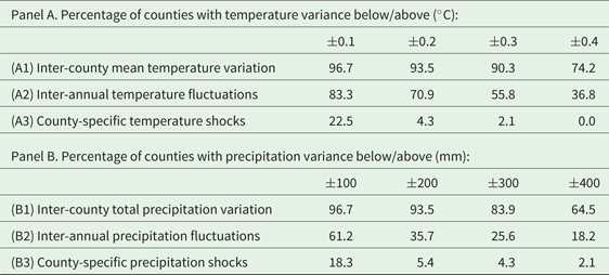
in which w _it is the weather outcome of county i in year t; T _i is the climate (i.e., long-term average weather outcome) of county i, which is assumed to be constant over time but differs across counties; d _t measures the inter-annual weather fluctuations that are common across counties in the same year but vary over time; and ε _it represents county-specific weather shocks.Footnote ¹² In a panel model with time fixed effects, the inter-annual weather fluctuations that are common across observations (d _t ) can be filtered out, and thus the remaining meteorological variation pertains only to cross-sectional climate differences (T _i ) and idiosyncratic local shocks (ε _it ). Since the local shocks are quite small (as shown in table 4), the impacts are mainly identified through cross-sectional climate differences, and therefore the long-run adaptations are included. On the other hand, the county fixed effect can be used to eliminate inter-county differences in climate T _i , which is constant over time, with the remaining variation pertaining only to common inter-annual weather fluctuations (d _t ) and county-specific weather shocks (ε _it ). Since the variation in county-specific weather shocks is very small, the impacts are mainly identified through the common inter-annual weather fluctuations and thus do not include adaptation benefits.

Table 4.

The magnitudes of inter-county climate (T _i ) variation, inter-annual weather fluctuations (d _t ), and local weather shocks (ε _it )

Note: Temperature is measured by the yearly mean temperature (^°C), while precipitation is measured by the yearly total precipitation (mm). The ‘inter-county mean temperature variation’ and the ‘inter-county total precipitation variation’ represent the climate (T _i ) differences, which are calculated as the deviation of the county mean from the sample mean. The ‘inter-annual temperature fluctuations’ and the ‘inter-annual precipitation fluctuations’ represent the weather fluctuations (d _t ), which are calculated as the deviation from the county mean. The ‘county-specific temperature shocks’ and the ‘county-specific precipitation shocks’ measure the variation in local shocks (ε _it ), which are calculated as the remaining variation after the county mean and the year mean are subtracted from each observation. All entries are calculated for the sample counties and sample years (2010–2012). See the text for further details.

Therefore, the difference of the impact identified from two panel models, one with time fixed effects and the other with county fixed effects, can be interpreted as the benefits of long-run adaptation. To show this, assume that A is the full set of adaptation methods that can be taken in the long run, and B is the full set of adaptation methods that can be taken in the short run. Considering that the adaptation methods that can be taken in the short run, such as shifting sowing time and using more pesticides, are most likely still available when dealing with the long-run climate change, we have B ⊂ A. We define the set of adaptation methods that can be taken only in the long run as C, so that C = A − B. The panel model with time fixed effects identifies the impact mainly through the cross-sectional climate differences (T _i ) and hence includes the benefits of A. The panel model with county fixed effects identifies the impact mainly though the year-to-year weather fluctuations (d _t ) and hence only includes the benefits of B. Therefore, their difference reflects the benefits of C, which are the full set of adaptation methods that can be taken only in the long run. As defined before, we refer to the benefits of C as the benefits of long-run adaptation.

Table 4 shows the actual size of the variation pertaining to ε _it , T _i , and d _t . Row (A1) shows that 74.2 per cent of the sample counties had deviations in their yearly mean temperature (T _i ) from the sample mean that were larger than 0.4^°C, while row (A3) shows that no counties had county-specific temperature shocks (ε _it ) higher than 0.4^°C. The same result applied to precipitation, with 64.5 per cent of the counties having more than 400 mm of deviation from the yearly total precipitation (T _i ) from the sample mean and only 2.1 per cent of counties having local precipitation shocks (ε _it ) of more than 400 mm (see rows (B1) and (B3)). Similarly, comparing rows (A3) and (B3) with rows (A2) and (B2), we find that the county-specific weather shocks are also negligible relative to the inter-annual weather fluctuations. These results support our argument that climate change impacts can be identified mainly through inter-county mean climate differences in a panel model with time fixed effects and through common inter-annual weather fluctuations in a panel model with county fixed effects.

However, since these climatic variables were calculated only for a three-year panel, it is likely that the small county-specific temperature and precipitation shocks, as shown in table 4, are the result of too short a panel period. To test this possibility, we calculated the values for the same variables as shown in table 4 using 30 years of weather data for the sample counties and found quite similar results. Since the magnitudes of inter-annual weather fluctuations were quite similar across regions, it is reasonable to find small county-specific weather shocks after removing the inter-county climate differences and the common inter-annual weather fluctuations. Similar results have been found in previous studies using US data (Fisher et al., Reference Fisher, Hanemann, Roberts and Schlenker2012).

The panel model used to identify climate change impact through cross-sectional climate differences is shown in equation (2), in which y _ijt denotes the crop profits per hectare of household i in county j and year t; C _it is a vector of county-level climate variables, including yearly DD, yearly HDD, yearly total precipitation, and their quadratic terms; L _ijt is a vector of the farm and household characteristics as shown in table 1, including capital intensity, land size, labor intensity, head of household education and age, disaster loss, and market access; K _jt is a vector of the soil quality, transportation conditions, and agricultural price index as defined in the last three rows of table 1; α, β, and γ are coefficients; and ρ _pt represents the province-by-year dummy. The dummy was used to filter out year-to-year weather and other fluctuations that were common across counties within each province.Footnote ¹³ Thus, the coefficients of the climate variables in this model were identified mainly through the inter-county mean climate differences, and the benefits of adaptations could then be included. Finally, in the estimation, the error term μ _it is clustered at the province level in order to address the potential bias from the spatial correlation of the error term (Deschênes and Greenstone, Reference Deschênes and Greenstone2007; Fisher et al., Reference Fisher, Hanemann, Roberts and Schlenker2012).

The model used to identify climate change impacts through inter-annual weather fluctuations is presented in equation (3). The settings for y _ijt , C _jt , L _ijt , and K _jt are the same as for equation (2). The only difference is in the use of fixed effects. Model (3) includes the county fixed effects τ _j to eliminate inter-county climate differences and does not use any type of time fixed effects, as these tend to eliminate most of the year-to-year weather fluctuations.Footnote ¹⁴ Thus, the climatic coefficients are mainly identified through the year-to-year weather fluctuations and do not include the benefits of adaptations. Finally, the error term υ _ijt is clustered at the province level.

By combining the estimates of the climate variables from models (2) and (3) with the climate change predictions, we were able to project the impacts with and without adaptations, respectively. The differences in the projected impacts between these two models can be interpreted as the benefits of long-run adaptation.

The most significant advantage of this approach is evaluating the value of long-run adaptations as a whole, thus freeing the analyst from the burden of estimating the value of each of the innumerable adaptive responses by farmers. This advantage is derived directly from the basic idea of the hedonic approach: obtaining information about adaptations to future climate change by examining the current production differences across climate regions.Footnote ¹⁵ Large cross-sectional climate differences are observed, and farmers should have adapted to the long-run climate of their regions.

A large body of studies has shown that climate has tremendous effects on agricultural production across regions, and most of the cross-sectional differences in agricultural production practices resulting from climatic differences can be explained as the result of farmers' long-run adaptation to the climate of their regions. Specifically, the distribution of crop types and crop varieties across regions are mainly the result of farmers' adaptive choices based on their long-run climate observations. Regional gradients of temperature result in the distribution of different crops and varieties from north to south (Cramer and Solomon, Reference Cramer and Solomon1993; Ramankutty et al., Reference Ramankutty, Foley, Norman and Mcsweeney2002), while for regions with sufficiently warm temperatures, cultivation is strongly determined by the distribution of precipitation.

Even though crop choice is critically dependent on climate, humans have adopted various other adaptive behaviors to overcome natural limitations to some extent. In response to the observed climate, farmers in different climate regions choose the optimal farm-management practices for their regions. For example, the sowing time in the temperate zones of northern China is much later than it is in the tropics of southern China so that crops have sufficiently warm temperatures during germination (Chen et al., Reference Chen, Hu and Yu2005); moreover, busting is usually chosen in southeast China where precipitation is abundant during the growing season, while conservation tillage measures are taken by farmers in northwest China where precipitation is quite limited (Zhang et al., Reference Zhang, Li, Yang, Wang and Chen2011). In modern agricultural production, additional adaptive measures are available that depend on intensive investments, such as the adoption of greenhouse and ground water irrigation systems to address insufficiency in growing season temperature and precipitation (Jin and Young, Reference Jin and Young2001; Thomas, Reference Thomas2008).

Even though climate differences and farmers' adaptive behaviors can explain many cross-sectional production differences, many other non-climatic factors also have significant effects. For example, differences in land quality and transportation also have significant effects on variations in agricultural profits. Nevertheless, cross-sectional climate differences can still be a useful instrumental variable for identifying the benefits of adaptation to future climate change. As suggested by Dell et al. (Reference Dell, Jones and Olken2014), non-climatic variables with the potential to influence agricultural profits and also correlate with climatic variables are themselves most likely the result of climate but not the cause of it. Omitting these variables will not necessarily result in biased estimates of the coefficients of climatic variables. Moreover, in our econometric analyses, we did our best to control for non-climatic determinants of agricultural profits, including capital intensity, land size, labor intensity, head of household education and age, market access, land quality, transportation, and price level.

4. Empirical results

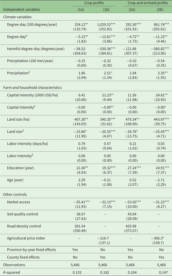
The regression results are shown in table 5. Columns (1a) and (1b) present the regression results from model (2) and model (3) respectively, using crop profits as the dependent variable, while columns (2a) and (2b) represent the regression results from model (2) and model (3) respectively, using the average profits of crops and orchards as the dependent variable.

Table 5.

Regression results of the effects of climatic variables and household characteristics on agricultural profits

Note: The definitions of the variables are given in table 1. Stand errors clustered at the province-level are reported in parentheses. Coefficients of soil quality control and road density control are omitted in columns (1b) and (2b) because these county-level variables are mainly time invariant and have been accounted for by the county fixed effects.

Significance levels are ***P < 0.01, **P < 0.05, * P < 0.1.

For all of the four regressions, the estimated coefficients of the yearly degree-day are statistically significant and show the inverted U-shaped relationship that is usually found in climate change impact studies and indicates agricultural profits increasing with degree-day up to a turning point, after which they decline. The coefficients of yearly harmful degree-day are all negative, reflecting the negative effect of extreme heat on agricultural production. It is not surprising to find that the coefficient of harmful degree-day is statistically insignificant in columns (1a) and (2a) because the province-by-year fixed effects applied tend to account for the extreme heat, which is likely part of the inter-annual weather fluctuations but not the climate normal in the sample areas.

The coefficients of precipitation are all statistically insignificant, presumably because the control variables, especially the fixed effects, account for a significant share of the effects of precipitation. Previous studies have generally found that precipitation is not a good measure of water supply for crops grown, especially for irrigated agriculture (Schlenker et al., Reference Schlenker, Hanemann and Fisher2005). In the data, the agricultural production of 78.0 per cent of households depends on irrigation.Footnote ¹⁶ Hence, the estimated effects of the predicted changes in precipitation are unreliable. Therefore, in the following calculation of the impacts of climate change and the benefits of adaptations, we mainly focus on the effects of warming.

Most of the control variables in these four regressions have statistically significant effects on profits per hectare. Specifically, profits per hectare increase with increasing capital intensity until a turning point, after which the effect becomes negative, but the negative effect is negligible (the coefficient of the square term is approximate to zero). The effect of land size on profits also shows an inverted U-shaped relationship. In addition, profits per hectare rise significantly with the education level of the head of household and the volume of irrigation water used, and decline significantly with losses due to natural disasters and the distance to market. All these significant effects are quite intuitive.

However, quantitatively, there is a difference between the estimated coefficients of models with and without long-run adaptations. For example, using the regression coefficients we calculate that the marginal effect at 4000 degree-day, which is approximately the average degree-day under scenario RCP4.5, is −0.87 for the model without adaptation and −0.59 for the model with adaptation. This suggests that with adaptation, the damage of warming on agricultural profits could be smaller on average. Similarly, according to the coefficient of harmful degree-day, the negative effect of extreme heat is weaker with adaptation than without, which implies that adaptation can help reduce the damage of extreme heat on agricultural production.

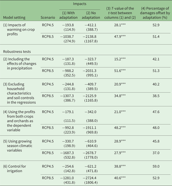
We combined the estimated coefficients of degree-day, degree-day square, and harmful degree-day of models (2) and (3) with the climate change scenarios to predict the impacts of warming with and without long-run adaptations, respectively. Row (1) of table 6 reports the predicted yearly impact of warming on crop profits per hectare by the end of this century for two scenarios. The model that did not include long-run adaptations predicted much more damage (column (2)) than the model that included long-run adaptations (column (1)) for both scenarios. The t-test as reported in column (3) found statistically significant differences between the estimated impacts with and without long-run adaptations.

Table 6.

Impacts of warming on crop profits by the end of this century and the benefits of long-run adaptation (2010 constant USD per hectare per year)

Note: Standard deviations are reported in parentheses.

Significance levels are *** P < 0.01. See the text for further details.

Specifically, under the most likely climate change scenario RCP4.5, the predicted changes in crop profits per hectare will be −193.8 USD and −412.1 USD with and without long-run adaptations, respectively. These damages correspond to 8.9 per cent and 18.9 per cent of the current mean annual profits per hectare in the sample area (see table 2). Column (4) reports the percentage of damages that will be offset by long-run adaptations. Long-run adaptations will help to mitigate 52.9 per cent and 51.4 per cent of the damages predicted by the model that did not include long-run adaptations for scenarios RCP4.5 and RCP8.5, respectively. In addition, relatively large standard deviations from the estimated damages were found, implying that there are significant regional differences in the impacts of warming.

The estimates of the impact of warming and the value of long-run adaptations are generally consistent with the literature. Previous hedonic studies, which include long-run adaptations, usually predict relatively small impacts of warming as in this paper. For example, under comparable climate change scenarios,Footnote ¹⁷ Wang et al. (Reference Wang, Mendelsohn, Dinar, Huang, Rozelle and Zhan2009) predict the yearly loss of net revenue for rainfed farms in China would be 256.5 USD per hectare (or 11.7 per cent), Wang et al. (Reference Wang, Huang, Zhang and Li2014) find the net crop revenue will decline by 12.9 percent in North China, and Zhou and Turvey (Reference Zhou and Turvey2014) predict the change of the output of rice, wheat, and maize in China ranges from +8.0 per cent to −10.6 per cent depending on the crop types and varieties. On the other hand, studies depending on simulation models, which generally exclude long-run adaptations, predict larger impacts of warming. For example, under comparable climate change scenarios, Xiong et al. (Reference Wei, Declan, Erda, Yinlong, Hui, Jinhe, Lan and Yan2009) predict a 18 per cent decrease in total grain output in China, Matthews et al. (Reference Matthews, Kropff, Horie and Bachelet1997) predict the rice yield in the major rice-growing regions of Asia will drop by 21 per cent, and Tao and Zhang (Reference Tao and Zhang2011) find decreases in the yields of irrigated maize range from 4.3 per cent to 32.1 per cent depending on the possibility of growing season shifting. Although previous studies do not predict the value of long-run adaptations in China, the differences between the impacts estimated from the hedonic studies and the simulation studies suggest that long-run adaptations can help to offset a significant share of the damage of warming.Footnote ¹⁸

Rows (2) to (5) of table 6 provide robustness tests. The main analysis as shown in row (1) only includes the effects of warming. In row (2), the effects of changes in precipitation are also included in the estimation. We find that including precipitation in the estimation does not significantly change the estimated impacts and adaptations. Both models estimated slightly smaller damages for each scenario, and adaptations are still expected to offset about half of the damages.

A potential concern of panel model (2), which depends on inter-county climate differences, is omitted-variable bias. Even though the inter-annual common fluctuations and the inter-province time-invariant differences are well controlled by the province-by-year fixed effects, we did not control for within-province inter-county differences apart from the controls listed in table 1. To test for potential omitted-variable bias, we dropped all household-level controls and the soil-quality control from the regression. As shown in row (3), the estimated benefits of long-run adaptation drop from 52.9 per cent to 40.2 per cent for scenario RCP4.5 and from 51.4 per cent to 38.5 per cent for scenario RCP8.5. The results are similar if we only exclude control subgroups. Since omitting all these crucial determinants of crop profits only reduces the adaptation benefits by about 12 per cent, the remaining omitted variables might not cause a large bias.

The main analysis only includes profits from annual crops. Because the responses of perennial plants to climate change might be different from those of annual crops, including the profits from orchards for which production is mainly dependent on perennial plants, the analysis might lead to a different adaption estimate. Row (4) of table 6 shows this possibility. The impacts are estimated from regressions that used the weighted average of profits from crops and orchards as the dependent variable. For the model with long-run adaptations, the estimated impacts are quite similar to the impacts on crop profits. However, the model without long-run adaptations predicted significantly smaller damage than that reported in row (1), presumably because perennial orchards are more resistant than annual crops to inter-annual weather fluctuations. As reported in the last column, long-run adaptations will still help to reduce a significant share of the damages (i.e., 47.6 per cent under scenario RCP4.5 and 48.0 per cent under scenario RCP8.5).

Since adjusting the growing season may be an important way of adapting to climate change, in the main analysis, we use yearly climatic variables instead of growing season climatic variables to allow for the adjustment of growing seasons in the long run. Intuitively, using growing season climatic variables in the estimation will underestimate the benefits of adaptation. In row (5), we provide the estimates using growing season climatic variables with a fixed growing season from March to October. As expected, the estimated benefits of adaptation drop to 45.8 per cent for scenario RCP4.5 and to 37.0 per cent for RCP8.5. The main conclusion remains that omitting long-run adaptations will dramatically overestimate the damages.

Irrigation has not been included as a control variable in the main analysis because it is an important adaptation to climate change. In places with higher temperature and lower precipitation, it is possible for farmers to use more irrigation water to reduce the negative effects of these unfavorable climate conditions. Therefore, if we control for irrigation in the model that depends on cross-section climate differences, the adaptation of irrigation will not be captured in the coefficients of climatic variables. On the other hand, since irrigation, which is an important determinant of agriculture profits, is not always available, excluding irrigation from the model may result in omitted variable bias. As a robustness check, row (6) of table 6 presents the estimation results from models that control for irrigation. We find that, comparing with row (1), including irrigation does not significantly change the estimated value of adaptation.

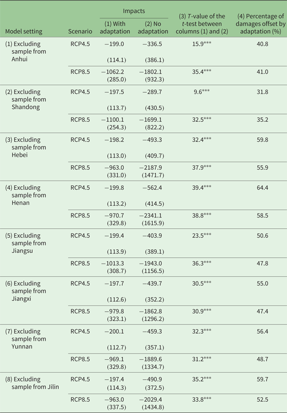
It is also interesting to check if the estimation results are sensitive to the study sample. To do so, we drop data from one province each time and re-do the estimation to generate 8 group of estimates. As presented in column (1) of table 7, the estimated damage from the model using cross-section climate variations is quite robust to this check. Specifically, the estimated loss of profit ranges from 197.4 to 199.8 under the scenario RCP4.5 and from 963.0 to 1062.2 under RCP8.5. This result suggests that omitted inter-province differences do not significantly affect the conclusion of this paper. In addition, as presented in the last column of table 7, although with noticeable variations, long-run adaptation will still help to offset at least one third of the damage of warming.

Table 7.

Testing the potential omitted variables bias by excluding samples for each province and reestimating the value of adaptation (2010 constant USD per hectare per year)

Note: Standard deviations are reported in parentheses.

Significance levels are *** P < 0.01. See the text for further details.

Finally, we investigated the effects of farm and household characteristics on the benefits of adaptation. We first calculated the impacts of warming predicted by RCP4.5 on crop profits for each household using the estimates from column (1a) and (1b) of table 5, respectively. Second, we calculated the household-level adaptation value as the difference in the impact estimated from these two models. Third, we performed a regression analysis of the household-level values of adaptation against the farm and household characteristics listed in table 1 and controlled for the mean temperature differences among counties. The significant regression coefficients are reported in equation (4):Footnote ¹⁹

We found that the cross-sectional adaptation value first decreased and then increased with the degree-day. In other words, very cold and very hot areas have higher adaptation values than temperate areas. This result is intuitive, because farmers in cold areas have more potential to adopt adaptation measures to exploit the beneficial opportunities of warming, while farmers in hot areas are more likely to take adaptation measures to moderate the negative effects of warming.

More importantly, both capital intensity and farmland size have statistically significant effects on the adaptation value. The coefficient of capital intensity suggests that 10 per cent increases in capital intensity from its current mean will raise the yearly benefits of adaptation by 124 USD per hectare. Hence, a government policy targeted at enhancing farmers' adaptive capacity can work by encouraging investment in the physical capital of agricultural production. On the other hand, the value of adaptation decreases with farmland size at first and then increases after the turning point, which is 5.4 hectares per household. If we increase the farmland managed by the average household by 1 hectare from its current mean, the yearly benefits of adaptation will drop by 104 USD per hectare. However, once the farmland size exceeds 5.4 hectares per household, further increases in farmland size will enhance adaptation benefits. A possible explanation is that, for small household farms in China, increasing farmland size means less labor can be input per hectare of land in response to warming. But once the land size is large enough, modern agricultural production methods such as mechanized agriculture production are available to reduce labor force constraints. Finally, an increase in the average farmer's age by one year will reduce the benefits of adaptation by 20.4 USD per hectare. This could reflect the fact that old farmers have less adaptation ability than young farmers.

5. Concluding remarks

This paper provides empirical support for the basic argument of the hedonic approach that omitting long-run adaptations will dramatically overestimate the damage of climate change. Depending on large-scale household-level survey data from rural China, the empirical results show that long-run adaptations are able to offset one third to one half of the damages of warming using various model settings and climate change scenarios. Hence, omitting long-run adaptations will dramatically overestimate the damages of warming. This study also finds that capital intensities and farmland size have significant effects on farmers' adaptive capacities.

There are several important caveats to the empirical results. First, the potential benefits from future technological advancements induced by climate change are not included in the estimation. Hence, this study estimates only the lower boundary of adaptation benefits. Second, forestry and animal husbandry were excluded from the survey. If it is possible for farmers to adapt to warming by switching land use among crops, animal husbandry, and forestry, this study would tend to underestimate the benefits of long-run adaptation. Third, in this partial equilibrium analysis, agricultural prices are assumed to be constant during climate change. This assumption is reliable if the positive effects in currently cold regions offset most of the negative effects in currently hot areas. Otherwise, agricultural prices will rise and the benefits of adaptation will be even greater. Finally, although the model suggests that long-run adaptations have the potential to significantly reduce the damage of warming, in the short-run, farmers will still be adapting to climate change and losses will be greater than what have been predicted by the model with long-run adaptations.