2.1 Suspension viscosity

Adding suspended particles to a fluid increases the effective viscosity of the mixture above that of the suspending fluid. This has been known for a Newtonian fluid since the work of Einstein (Reference Einstein1906), with a correction of Einstein (Reference Einstein1911), who gave the expression $\unicode[STIX]{x1D702}_{f}(1+5\unicode[STIX]{x1D719}/2)$ for the viscosity of a dilute suspension of rigid spheres, where $\unicode[STIX]{x1D702}_{f}$ is the viscosity of the solvent and $\unicode[STIX]{x1D719}$ is the volume fraction of the spheres. (The viscosity was initially found to be $\unicode[STIX]{x1D702}_{f}(1+\unicode[STIX]{x1D719})$ by Einstein (Reference Einstein1906). Einstein was later informed of the viscosity measurements performed by Bacelin under the supervision of Perrin, which were significantly larger than his initial prediction. He then asked Hopf to check his calculation and an error was found. The exact expression, $\unicode[STIX]{x1D702}_{f}(1+5\unicode[STIX]{x1D719}/2)$ , was finally given by Einstein (Reference Einstein1911).) Einstein calculated this viscosity by considering the effect of immersing a single solid spherical particle in a linear shear flow. Just looking at the flow around this single particle provides some hint of the physical origin of this increase in viscosity. The particle is considered to be freely suspended in the shearing flow, which means that the sphere experiences no hydrodynamic force or torque. In practice, this can be achieved by considering a neutrally buoyant particle, i.e. a particle having the same density as the fluid. The ambient shearing flow can be decomposed into a rotational and a straining flow (see figure 2). The sphere freely rotates in the rotational portion of the flow and this freely rotating sphere embedded in a solid-body rotation creates no disturbance. The rigid sphere, however, resists the straining component of the shearing flow and this produces a disturbance flow that leads to an increase in the rate of viscous dissipation. In simple terms, the viscosity is increased because of the resistance of the non-deforming particle to the straining component of the shearing flow.

Figure 2.

Decomposition of a sphere in shear by combining a sphere in rotation plus a sphere in strain. The sphere is considered as ‘freely mobile’, i.e. it experiences no hydrodynamic force or torque. The disturbance flow generated by the sphere in shear is solely due to its resistance to the straining component of the shearing flow since the freely rotating sphere embedded in solid-body rotation creates no disturbance. This disturbance flow leads to an increase in the rate of energy dissipation and thus to an increase in viscosity.

A granular suspension of monodisperse spheres, i.e. a suspension of non-colloidal, monodisperse, hard spheres, can be seen as the simplest case of suspensions. In these conditions, there are no Brownian or colloidal forces (such as electric double layer or van der Waals forces, i.e. all the forces that are not hydrodynamic or frictional contact interactions and are expected to be important for small particles) that can drive the suspension to a well-defined rest state when the flow is stopped and therefore no relaxation process with an intrinsic time scale. For now, we also restrict the discussion to the condition of vanishingly small Reynolds numbers (inertial suspensions are addressed in § 7.4). When this suspension of neutrally buoyant hard spheres is subjected to a steady shear flow, the linearity of the Stokes equations implies that the shear stress $\unicode[STIX]{x1D70F}$ scales linearly with the shear rate $\dot{\unicode[STIX]{x1D6FE}}$ . In other words, the scaling of the stress is viscous, $\unicode[STIX]{x1D70F}=\unicode[STIX]{x1D702}_{s}\unicode[STIX]{x1D702}_{f}\dot{\unicode[STIX]{x1D6FE}}$ , where $\unicode[STIX]{x1D702}_{s}$ is termed the relative viscosity of the suspension. Moreover, dimensional analysis indicates that, for this Stokesian non-colloidal suspension, there is only a single remaining independent variable, the volume fraction of particles, $\unicode[STIX]{x1D719}$ . The relative viscosity, $\unicode[STIX]{x1D702}_{s}$ , is thus solely a function of $\unicode[STIX]{x1D719}$ , i.e. $\unicode[STIX]{x1D702}_{s}=\unicode[STIX]{x1D702}_{s}(\unicode[STIX]{x1D719})$ . This viscosity is independent of the shear rate and has a unique value at every concentration. Hence, the suspension can be seen as Newtonian with a viscosity increasing with increasing volume fraction.

Figure 3.

Rheometry used for measuring the viscosity of suspensions. (a) Cone-and-plate rotational rheometer. The fluid sample is put between the cone and plate and, when the cone angle $\unicode[STIX]{x1D6FC}$ is small enough ( $\unicode[STIX]{x1D6FC}\leqslant 0.1$  rad), the viscosity is given by $\unicode[STIX]{x1D702}=3\unicode[STIX]{x1D6FC}T/(2\unicode[STIX]{x03C0}R^{3}\unicode[STIX]{x1D6FA})$ , where $R$ is the radius of the cone and the plate and $T$ and $\unicode[STIX]{x1D6FA}$ are the measured torque and rotational velocity, respectively. (b) Parallel-plate rotational rheometer. The fluid sample is put inside the gap, $h$ , between the two plates and the viscosity based on a Newtonian fluid assumption is given by $\unicode[STIX]{x1D702}=2Th/(\unicode[STIX]{x1D6FA}\unicode[STIX]{x03C0}R^{4})$ , where again $T$ and $\unicode[STIX]{x1D6FA}$ are the measured torque and rotational velocity, respectively. (c) Couette rotational rheometer. The fluid sample is put inside the annular gap between the two coaxial cylinders and, when the gap is small enough (i.e. the radius of the cup $R_{c}$ and that of the bob $R_{b}$ are very close, $R_{b}/R_{c}>0.99$ ), the viscosity is given by $\unicode[STIX]{x1D702}=T(R_{c}-R_{b})/[\unicode[STIX]{x03C0}L\unicode[STIX]{x1D6FA}(R_{c}+R_{b})R_{b}^{2}]$ , where $L$ is the length of the cylinders and $T$ and $\unicode[STIX]{x1D6FA}$ are again the measured torque and rotational velocity, respectively. (d) Inclined plane rheometer. The fluid flows down an inclined plane at an angle $\unicode[STIX]{x1D703}$ with the horizontal and (within the assumption of a Newtonian behaviour) measuring its free surface velocity, $u_{surface}$ , and its height, $h$ , yields the viscosity $\unicode[STIX]{x1D702}=\unicode[STIX]{x1D70C}gh^{2}\sin \unicode[STIX]{x1D703}/(2u_{surface})$ , where $\unicode[STIX]{x1D70C}$ is the fluid density.

Measuring the viscosity of suspensions may prove to be challenging as it requires a specific procedure and analysis. Problems such as the wall-slip effect, sedimentation or creaming (i.e. particles having a density higher or lower, respectively, than the suspending liquid), and particle migration (shear-induced migration will be considered in § 3.3.1) can hamper the measurements. Macroscopic viscosity measurements using classical rotational rheometers such as cone-and-plate, parallel-plate and Couette rheometers have been commonly used (see figure 3). Macroscopic viscosimetry has also been achieved with the less known inclined-plane rheometer, which permits the exploration of a larger $\unicode[STIX]{x1D719}$ range (flow of suspensions along an inclined plane will be further discussed in § 4.2.1). To overcome problems such as concentration inhomogeneities due in particular to the migration phenomenon, local measurements can be performed using non-intrusive techniques such as magnetic resonance imaging (MRI) or ultrasound coupled to a classical rheometer. The extensive measurements performed for non-colloidal hard spheres show that the suspension viscosity increases with increasing $\unicode[STIX]{x1D719}$ and diverges at a jamming transition where the particle concentration reaches a maximum value, $\unicode[STIX]{x1D719}_{c}$ , for which the suspensions cease to flow (see figure 4 a).

This maximum flowable volume fraction generally differs from the maximum close random packing fraction ( ${\approx}0.64$ ) that can be obtained by vibrating or repeated tapping and in practice it may be difficult to flow a suspension for $\unicode[STIX]{x1D719}\gtrsim 0.55{-}0.62$ . The precise value of $\unicode[STIX]{x1D719}_{c}$ varies depending on the size distribution of the particles and also their surface interactions – more precisely their frictional interactions (this jamming transition of suspensions under constant shear will be discussed in § 5.3). By using the reduced volume fraction, $\unicode[STIX]{x1D719}/\unicode[STIX]{x1D719}_{c}$ , with appropriate values for $\unicode[STIX]{x1D719}_{c}$ , the plots of viscosity versus concentration can be collapsed onto a master curve, as shown in figure 4(b) for a selection of data coming from both macroscopic and local measurements using different combinations of monodisperse hard spheres and Newtonian fluids. We have also added to these plots the data of Boyer, Guazzelli & Pouliquen (Reference Boyer, Guazzelli and Pouliquen2011a ) and of Dagois-Bohy et al. (Reference Dagois-Bohy, Hormozi, Guazzelli and Pouliquen2015) coming from pressure-imposed rheometry, which will be discussed in § 4.1.

The linear dependence in $\unicode[STIX]{x1D719}$ given by the Einstein relative viscosity ( $=1+5\unicode[STIX]{x1D719}/2$ ) only reproduces the viscosity curve in the very dilute regime, i.e. up to a volume fraction of approximately 0.05, as can be seen in figure 4. For larger $\unicode[STIX]{x1D719}$ , the interactions between particles cannot be neglected. For instance, at $\unicode[STIX]{x1D719}\approx 0.1$ , the average distance between particles having a diameter $d$ is $d/2\unicode[STIX]{x1D719}^{1/3}\approx d$ , and therefore neighbouring particles are affected by their respective disturbance flows. This pair interaction effect is expected to yield a viscosity contribution of $O(\unicode[STIX]{x1D719}^{2})$ . However, the long-range nature of these velocity disturbances makes the calculation of this contribution difficult. The disturbance flow created by a freely suspended sphere in a shearing flow decreases at leading order as $1/r^{2}$ , where $r$ is the radial distance to the centre of the sphere. It can be shown that this results in an incremental stress on a neighbouring sphere of order $O(1/r^{3})$ . A simple integration over the volume of the suspension assuming a uniform pair distribution function leads unfortunately to a diverging integral and a special method known as hydrodynamic renormalisation must be employed (Batchelor & Green Reference Batchelor and Green1972a ,Reference Batchelor and Green b ). The expression up to terms of order $O(\unicode[STIX]{x1D719}^{2})$ for a pure straining flow is $\unicode[STIX]{x1D702}_{s}=1+5\unicode[STIX]{x1D719}/2+6.95\unicode[STIX]{x1D719}^{2}$ . For a shearing flow, there is a complication in defining the pair probability because of the existence of closed trajectories due to the rotational portion of the shearing flow. Assuming a random microstructure leads to a smaller coefficient ( ${\approx}5$ ) of $\unicode[STIX]{x1D719}^{2}$ . This latter expression seems to agree reasonably with the experimental data in the semi-dilute regime (up to $\unicode[STIX]{x1D719}\approx 0.10{-}0.15$ ) but fails to capture the rapid growth in viscosity observed when $\unicode[STIX]{x1D719}$ is further increased (see figure 4).

Figure 4.

Relative viscosity, $\unicode[STIX]{x1D702}_{s}$ , versus (a) volume fraction, $\unicode[STIX]{x1D719}$ , and (b) reduced volume fraction, $\unicode[STIX]{x1D719}/\unicode[STIX]{x1D719}_{c}$ . Experiments: of Boyer et al. (Reference Boyer, Guazzelli and Pouliquen2011a ) using pressure-imposed rheometry with polystyrene (PS) spheres of diameter $d=580~\unicode[STIX]{x03BC}\text{m}$ suspended in polyethylene glycol-ran-propylene glycol monobutyl ether as well as poly(methyl methacrylate) (PMMA) spheres of diameter $d=1100~\unicode[STIX]{x03BC}\text{m}$ suspended in a Triton X-100/water/zinc chloride mixture; of Bonnoit et al. (Reference Bonnoit, Darnige, Clement and Lindner2010) using an inclined plane rheometer tilted at two different angles with PS spheres of diameter $d=40~\unicode[STIX]{x03BC}\text{m}$ suspended in silicone oil; of Dagois-Bohy et al. (Reference Dagois-Bohy, Hormozi, Guazzelli and Pouliquen2015) using pressure-imposed rheometry with PS spheres of diameter $d=580~\unicode[STIX]{x03BC}\text{m}$ suspended in polyethylene glycol-ran-propylene glycol monobutyl ether; of Dbouk, Lobry & Lemaire (Reference Dbouk, Lobry and Lemaire2013) using a parallel-plate rotational rheometer with PS spheres of diameter $d=140~\unicode[STIX]{x03BC}\text{m}$ suspended in a mixture of water, UCON oil and zinc bromide; of Ovarlez, Bertrand & Rodts (Reference Ovarlez, Bertrand and Rodts2006) using MRI technique and a wide-gap Couette geometry with PS spheres of diameter $d=290~\unicode[STIX]{x03BC}\text{m}$ suspended in silicone oil; and of Zarraga, Hill & Leighton (Reference Zarraga, Hill and Leighton2000) using a parallel-plate rotational rheometer with glass spheres of diameter $d=44~\unicode[STIX]{x03BC}\text{m}$ suspended in three different fluids. Numerical simulations: of Sierou & Brady (Reference Sierou and Brady2002) and Gallier et al. (Reference Gallier, Lemaire, Peters and Lobry2014) with ( $\unicode[STIX]{x1D707}_{p}=0.5$ ) and without ( $\unicode[STIX]{x1D707}_{p}=0$ ) friction; as well as those of Mari et al. (Reference Mari, Seto, Morris and Denn2014) with ( $\unicode[STIX]{x1D707}_{p}=1$ ) and without ( $\unicode[STIX]{x1D707}_{p}=0$ ) friction, where $\unicode[STIX]{x1D707}_{p}$ is the friction coefficient between the spheres. Viscosity laws: of Einstein (Reference Einstein1906, Reference Einstein1911), of Batchelor & Green (Reference Batchelor and Green1972b ), of Krieger with exponent $\unicode[STIX]{x1D6FC}=-2.5\unicode[STIX]{x1D719}_{c}$ and $\unicode[STIX]{x1D6FC}=-2$ (Maron–Pierce), and of Eilers (Stickel & Powell Reference Stickel and Powell2005). The corresponding $\unicode[STIX]{x1D719}_{c}$ used for each set of data in panel (b) are indicated in the legend.

Computing the viscosity for larger $\unicode[STIX]{x1D719}$ is very difficult as multi-body hydrodynamic interactions must be computed together with determining the microstructure. Another complexity is that the spheres can interact not only by hydrodynamic interactions through the liquid but also by direct mechanical contact. Exact analytic calculations do not exist, and in order to tackle this concentrated regime simulations with various levels of approximation and sophistication have been performed, starting with the now-classical Stokesian dynamics, which uses the properties of the Stokes equations through computing the resistance and mobility functions, and going to the more recent direct numerical simulations using lattice-Boltzmann or fictitious domains methods. The accelerated Stokesian dynamics simulations of Sierou & Brady (Reference Sierou and Brady2002) that consider the shearing flow of a suspension of 512 hard spheres with a repulsive interparticle force to prevent overlap are reported in figure 4, together with the more recent fictitious-domain simulations of Gallier et al. (Reference Gallier, Lemaire, Peters and Lobry2014) that solve the long-range hydrodynamics and lubrication interactions for ${\approx}600{-}1000$ spheres and also incorporate a discrete element method to model contact forces (this contact model assumes a Hertz law and includes roughness and friction). An important outcome is that friction has a major impact as it is seen to increase the value of $\unicode[STIX]{x1D702}_{s}$ , in better agreement with the experimental data.

Frictional contacts between particles exist at lower $\unicode[STIX]{x1D719}$ , as will be pointed out later in § 5.1, but become essential to the rheology of the suspensions at large $\unicode[STIX]{x1D719}$ (typically $\unicode[STIX]{x1D719}\gtrsim 0.20$ ). For these large volume fractions, frictional contact forces overrun the long-range hydrodynamic interactions in such a way that it is no longer necessary to include these long-range interactions to obtain realistic predictions. This is evidenced in the simulations of Mari et al. (Reference Mari, Seto, Morris and Denn2014), which account for frictional contact forces along with viscous lubrication only (see figure 4). These simulations extend the previous numerical predictions for values of $\unicode[STIX]{x1D719}\geqslant 0.45$ . There are clearly two $\unicode[STIX]{x1D702}_{s}(\unicode[STIX]{x1D719})$ curves (the open stars and open crosses, respectively) which diverge at $\unicode[STIX]{x1D719}_{c}^{\unicode[STIX]{x1D707}_{p}\neq 0}\approx 0.60$ and at $\unicode[STIX]{x1D719}_{c}^{\unicode[STIX]{x1D707}_{p}=0}\approx 0.64$ (at random close packing fraction) for frictional and frictionless particles, respectively. Note that the friction coefficient between the spheres is $\unicode[STIX]{x1D707}_{p}=1$ in the simulations of Mari et al. (Reference Mari, Seto, Morris and Denn2014) while it is $\unicode[STIX]{x1D707}_{p}=0.5$ for those of Sierou & Brady (Reference Sierou and Brady2002) and Gallier et al. (Reference Gallier, Lemaire, Peters and Lobry2014), resulting in slightly larger values of $\unicode[STIX]{x1D702}_{s}$ for the data of Mari et al. (Reference Mari, Seto, Morris and Denn2014) and a divergence at a slightly lower packing fraction ( ${\approx}0.58$ rather than ${\approx}0.61$ ). The better agreement of the simulations including friction with the experimental observations implies that the non-colloidal hard spheres are indeed experiencing frictional contacts in experiments. As will be seen later in §§ 5.3 and 7.2, friction also plays a major role in the understanding of jamming and discontinuous shear thickening.

At this stage of the discussion, it is worth returning to the dimensional analysis introduced earlier in this section and emphasise that contact forces do not bring any additional force scale with which to compare the hydrodynamic force, as hard-sphere contacts can resist any applied load. This is valid whether the hard spheres are frictionless or frictional, as friction does not generate an additional force either. Therefore, the stress of suspensions of non-colloidal, frictional, hard spheres should scale viscously in Stokes flows and there should not be any shear-rate dependence of the viscosity.

Finally, to be comprehensive on the viscosity of suspensions, it is important to mention the numerous phenomenological equations relating the suspension viscosity to the volume fraction that can be found in the literature. Some of these expressions stem from mean-field approaches. They generally recover the Einstein viscosity limit at low concentration and aim to account for the divergence of the viscosity at $\unicode[STIX]{x1D719}_{c}$ . One of the most popular is the Krieger viscosity, $(1-\unicode[STIX]{x1D719}/\unicode[STIX]{x1D719}_{c})^{\unicode[STIX]{x1D6FC}}$ . The Einstein viscosity is recovered with an exponent $\unicode[STIX]{x1D6FC}=-2.5\unicode[STIX]{x1D719}_{c}$ but it does not fit properly the data at higher volume fractions, for which an exponent $\unicode[STIX]{x1D6FC}=-2$ yields better results (this latter expression is also known as the Maron–Pierce correlation); see figure 4. Another interesting correlation is that of Eilers, $[1+(5\unicode[STIX]{x1D719}/4)/(1-\unicode[STIX]{x1D719}/\unicode[STIX]{x1D719}_{c})]^{2}$ , which happens to comply with both high- and low-concentration limits and is in fairly good agreement with the experimental observations over the whole range of  $\unicode[STIX]{x1D719}$ .

2.2 Normal-stress differences

This quasi-Newtonian behaviour of the shear stress introduced in the preceding section does not fully describe the rheology of suspensions. Indeed, it does not account for the existence of normal-stress differences, i.e. for normal stresses that are no longer isotropic under shear, which appear for non-dilute suspensions. Since the suspension is incompressible, the pressure, i.e. the trace of the total suspension stress denoted $\unicode[STIX]{x1D72E}$ , is of no rheological interest as it is prescribed by the flow and the two pertinent quantities are the first and second normal-stress differences, which are defined as $N_{1}=\unicode[STIX]{x1D6F4}_{22}-\unicode[STIX]{x1D6F4}_{11}$ and $N_{2}=\unicode[STIX]{x1D6F4}_{22}-\unicode[STIX]{x1D6F4}_{33}$ , respectively, where the flow, the gradient and the vorticity directions are labelled $1$ , $2$ and $3$ (see figure 5). Similarly to the shear stress, these normal stresses scale viscously in Stokes flows. Since the normal stresses do not depend on the sign of the shear rate, the normal-stress differences are proportional to the modulus of the shear stress, $|\unicode[STIX]{x1D70F}|$ . They can be written as $N_{1}=\unicode[STIX]{x1D6FC}_{1}|\unicode[STIX]{x1D70F}|$ and $N_{2}=\unicode[STIX]{x1D6FC}_{2}|\unicode[STIX]{x1D70F}|$ . The ratios of normal-stress differences to shear stress, $\unicode[STIX]{x1D6FC}_{1}$ and $\unicode[STIX]{x1D6FC}_{2}$ , are called the normal-stress difference coefficients. They are solely functions of $\unicode[STIX]{x1D719}$ and do not diverge at $\unicode[STIX]{x1D719}_{c}$ since the normal-stress differences and the shear stress present the same divergence when approaching the jamming point at $\unicode[STIX]{x1D719}_{c}$ (Morris & Boulay Reference Morris and Boulay1999).

Figure 5.

Sketch of the pair interactions between spheres under simple shear. (a) For perfectly smooth spheres, the trajectories exhibit a fore–aft symmetry. (b) For rough spheres, the trajectories are irreversible and asymmetric. In that latter case, when the minimum approach distance for the pair is smaller than the roughness, the spheres enter into contact in the compressional region of the flow (upper left and bottom right quadrants) and move apart in the extensional region (upper right and bottom left quadrants), leading to a region depleted in particles (areas shaded dark) and thus to weaker hydrodynamic interactions in this extensional region. After the collision, the spheres do not come back to their initial streamlines, but lay on two critical streamlines shifted by a minimum approach distance corresponding to the roughness.

This non-Newtonian feature is intimately linked to the loss of isotropy of the suspension microstructure, which will be further discussed in § 5.1. Looking at the pair interactions between two spheres under simple shear offers some basic physical understanding of the development of these normal-stress differences (see figure 5). The trajectories of two perfectly smooth spheres are reversible and symmetric, as this motion reflects the fore–aft symmetry of the flow lines around a single sphere due to the reversibility of the Stokes flow (see figure 5 a). Whereas this pair motion creates additional shear stress as seen in the preceding section, it does not lead to normal-stress differences, as the effects of the compressive and extensive portions of the flow cancel. However, these reversible trajectories are extremely sensitive to contact perturbations. If the spheres present some surface roughness, the trajectories become irreversible and asymmetric, resulting in non-isotropic normal stresses (see figure 5 b). The spheres can collide in the compressional region of the flow when the minimum approach distance for the pair is smaller than the roughness. After the collision, the spheres do not come back to their initial streamlines but move apart, leading to a region depleted in particles in the extensional region. This crude sketch suggests that the normal stresses come from the repulsion between the two spheres as they approach one another in the shear. Since most of the collisions take place in the plane of shear, one expects $N_{2}$ to be negative. The sign of $N_{1}$ , as we will see in the following, is more uncertain but this simple description suggests that the deficit in hydrodynamic interactions at the rear of the collision (i.e. in the extensional region) leads to a negative  $N_{1}$ .

Figure 6.

Rheometry used for measuring normal-stress differences of suspensions. (a) Cone-and-plate rotational rheometer. Measuring the normal force acting on the upper plate yields a direct measure of the first normal-stress difference, $N_{1}$ . (b) Parallel-plate rotational rheometer. Measuring the normal force acting on the upper plate gives the difference between the first and second normal-stress differences, $N_{1}-N_{2}$ . (c) Parallel-plate rheometer with differential pressure transducers fitted flush against the lower plate surface. Measuring the radial profile of the normal stress along the velocity gradient direction yields $N_{2}+N_{1}/2$ and $N_{1}+N_{2}$ and thus the determination of both $N_{1}$ and  $N_{2}$ . (d) Weissenberg, or rotating rod, flow. Measurement of the free-surface deflection induced by the anisotropic stresses (rod dipping in the case of suspensions) provides the linear combination $N_{2}+N_{1}/2$ . (e) Tilted-trough flow. Measurement of the free-surface deflection induced by the second normal-stress difference (a bulge in the middle) yields a direct determination of  $N_{2}$ .

Normal-stress differences are difficult to measure as they happen to be much smaller than the shear stress for $\unicode[STIX]{x1D719}\lesssim 0.2$ . Standard rheological tools such as cone-and-plate or parallel-plate rotational rheometers have been used but also adapted, e.g. with pressure measurements at the wall (Singh & Nott Reference Singh and Nott2003; Dbouk et al. Reference Dbouk, Lobry and Lemaire2013), to enhance accuracy (see figure 6). Alternative approaches have also been undertaken to infer the normal-stress differences from measurements of the deflection of the free surface in a Weissenberg, or rotating-rod, geometry and in a tilted trough. The first method is well known in polymers as the Weissenberg or rod-climbing effect. For suspensions of spheres, the climbing is down instead of up the rod, and measurement of the free-surface profile provides a combination of the normal-stress differences. The second tilted-trough method provides the second normal-stress difference in isolation. These methods have some significant advantages over using a standard rheometer as confinement effects can be reduced and sensitivity improved (Boyer, Pouliquen & Guazzelli Reference Boyer, Pouliquen and Guazzelli2011b ; Couturier et al. Reference Couturier, Boyer, Pouliquen and Guazzelli2011; Dai et al. Reference Dai, Bertevas, Qi and Tanner2013). Using these non-conventional rheological tools (rotating rod and tilted trough) in conjunction (Boyer et al. Reference Boyer, Pouliquen and Guazzelli2011b ; Couturier et al. Reference Couturier, Boyer, Pouliquen and Guazzelli2011) or combining them with conventional rheometry (Zarraga et al. Reference Zarraga, Hill and Leighton2000; Dai et al. Reference Dai, Bertevas, Qi and Tanner2013) yields a complete measurement of the two differences, $N_{1}$ and $N_{2}$ , which have both been shown to be linear in the modulus of the shear stress, $|\unicode[STIX]{x1D70F}|$ . Most of the measurements available in the literature are collected in figure 7.

Figure 7.

Normal-stress difference coefficients, (a) $\unicode[STIX]{x1D6FC}_{1}$ and (b) $\unicode[STIX]{x1D6FC}_{2}$ , versus volume fraction, $\unicode[STIX]{x1D719}$ . Experiments: of Zarraga et al. (Reference Zarraga, Hill and Leighton2000) combining rotating-rod and parallel-plate measurements with glass spheres of diameter $d=44~\unicode[STIX]{x03BC}\text{m}$ ; of Singh & Nott (Reference Singh and Nott2003) using a cylindrical Couette and parallel-plate rheometers with PMMA spheres of diameter $d=196~\unicode[STIX]{x03BC}\text{m}$ ; of Boyer et al. (Reference Boyer, Pouliquen and Guazzelli2011b ) and Couturier et al. (Reference Couturier, Boyer, Pouliquen and Guazzelli2011) combining the rotating-rod and tilted-trough methods with PS spheres of diameters $d=70$ and $140~\unicode[STIX]{x03BC}\text{m}$ ; of Dai et al. (Reference Dai, Bertevas, Qi and Tanner2013) combining tilted-trough and parallel-plate measurements with PS spheres of diameter $d=40~\unicode[STIX]{x03BC}\text{m}$ ; and of Dbouk et al. (Reference Dbouk, Lobry and Lemaire2013) using wall-pressure measurements in a parallel-plate geometry with PS spheres of diameters $d=40$ and $140~\unicode[STIX]{x03BC}\text{m}$ . Numerical simulations: of Sierou & Brady (Reference Sierou and Brady2002) and Gallier et al. (Reference Gallier, Lemaire, Peters and Lobry2014) with ( $\unicode[STIX]{x1D707}_{p}=0.5$ ) and without ( $\unicode[STIX]{x1D707}_{p}=0$ ) friction and with confinement (bounded) in the frictional case. The dotted line in (b) is the $O(\unicode[STIX]{x1D719}^{2})$ theoretical prediction of Wilson (Reference Wilson2005). The $O(\unicode[STIX]{x1D719}^{3})$ correlations of Dai et al. (Reference Dai, Bertevas, Qi and Tanner2013) are also shown (dashed lines).

In spite of uncertainties and scatter in the data, some firm conclusions can be drawn for $N_{2}$ . The second normal-stress difference is found to be negative and its magnitude is seen to increase with increasing $\unicode[STIX]{x1D719}$ , growing especially quickly for $\unicode[STIX]{x1D719}\gtrsim 0.20$ to reach a magnitude of ${\approx}0.4|\unicode[STIX]{x1D70F}|$ at $\unicode[STIX]{x1D719}=0.5$ (see figure 7 b). The properties of the first normal-stress difference are more elusive. The magnitude of $N_{1}$ is unquestionably much smaller than that of $N_{2}$ , but assessing the sign is difficult (see figure 7 a). Some experiments find that $N_{1}$ is quite small and negative (Zarraga et al. Reference Zarraga, Hill and Leighton2000; Singh & Nott Reference Singh and Nott2003; Dai et al. Reference Dai, Bertevas, Qi and Tanner2013), while others report positive values (Dbouk et al. Reference Dbouk, Lobry and Lemaire2013), and yet others consider that the value is too close to zero to determine whether it is negative, positive or zero within experimental accuracy (Boyer et al. Reference Boyer, Pouliquen and Guazzelli2011b ; Couturier et al. Reference Couturier, Boyer, Pouliquen and Guazzelli2011).

Analytical calculations of the pair interactions of hard spheres have been conducted in the dilute regime (Wilson Reference Wilson2005) and predict that $\unicode[STIX]{x1D6FC}_{2}$ is proportional to $\unicode[STIX]{x1D719}^{2}$ with a proportionality coefficient that varies with surface roughness or minimum separation (this coefficient goes to zero for smooth spheres, i.e. assessing that $\unicode[STIX]{x1D6FC}_{2}=0$ in that latter case). This $O(\unicode[STIX]{x1D719}^{2})$ prediction has been reported for a roughness relative to the particle radius of $10^{-3}$ (which is typically measured experimentally) in figure 7(b). It is of the same order of magnitude as the experimental data for $\unicode[STIX]{x1D719}\lesssim 0.25$ but cannot capture the strong increase in magnitude observed for larger $\unicode[STIX]{x1D719}$ . Again, only numerical simulations can address the concentrated regime. The accelerated Stokesian dynamics simulations of Sierou & Brady (Reference Sierou and Brady2002) and fictitious-domain simulations of Gallier et al. (Reference Gallier, Lemaire, Peters and Lobry2014) presented earlier for the viscosity have been reported in figure 7. Again, friction between the particles has a profound impact on the rheology, as it increases the magnitude of $\unicode[STIX]{x1D6FC}_{2}$ and decreases that of $\unicode[STIX]{x1D6FC}_{1}$ , in better agreement with the available observations. An important finding revealed by the simulations of Gallier et al. (Reference Gallier, Lemaire, Peters and Lobry2014) is that the two normal-stress differences have different physical origins, as will be discussed further in § 5.2. The first difference $N_{1}$ is mostly of hydrodynamic origin, whereas the second $N_{2}$ comes from the contact interactions. These simulations also provide some hints to explain the discrepancies among observations for $N_{1}$ . Simulations performed in a wall-bounded shear flow show wall-induced layering of the particles, which has a moderate impact on $\unicode[STIX]{x1D6FC}_{2}$ but significantly affects $\unicode[STIX]{x1D6FC}_{1}$ (Gallier et al. Reference Gallier, Lemaire, Lobry and Peters2016) (see figure 7). Confinement together with friction can lead to positive value of $\unicode[STIX]{x1D6FC}_{1}$ , in closer agreement with the experiments of Dbouk et al. (Reference Dbouk, Lobry and Lemaire2013), where pressure measurements are taken at the lower plate of the rheometer cell.

The overall picture is that $N_{2}$ is large and negative, as most of the repulsive collisions between spheres happen in the plane of shear, while $N_{1}$ is small because the collisions happen fairly equally in the flow and the flow-gradient directions. However, the flow-induced microstructure of the frictional spheres can explain the sign of $N_{1}$ . In the suspension bulk, the deficit in hydrodynamic interactions in the extensional region leads to a negative sign, whereas, near a wall, the particle layering results in a decrease of contact stresses (enhanced by friction) and thus promotes a positive sign (at least for $\unicode[STIX]{x1D719}\lesssim 0.5$ as documented in figure 7; for larger $\unicode[STIX]{x1D719}$ other behaviour may be seen but there is not enough data to conclude yet).

2.3 Other non-Newtonian phenomena

The fundamental results that have been described up to now are that suspensions of non-colloidal hard spheres can be described by a single viscosity that is solely a function of volume fraction but also possess some non-Newtonian features since they develop non-isotropic normal stresses. Since there is no other force scale than the hydrodynamic forces, one expects rate-independent properties. Nonetheless, some shear-thinning behaviour has been reported in the concentrated regime starting at $\unicode[STIX]{x1D719}\approx 0.45{-}0.5$ (see e.g. Zarraga et al. Reference Zarraga, Hill and Leighton2000). This is not well understood and clearly implies that some additional forces come into play (shear-thinning behaviour is also observed for dense suspensions of fibres as discussed in § 7.1). This may also explain the differences in $\unicode[STIX]{x1D702}_{s}(\unicode[STIX]{x1D719})$ and $\unicode[STIX]{x1D6FC}_{1}(\unicode[STIX]{x1D719})$ or $\unicode[STIX]{x1D6FC}_{2}(\unicode[STIX]{x1D719})$ curves across experimental work for large  $\unicode[STIX]{x1D719}$ .

Another cause of scatter may be due to differences in frictional particle contact across samples resulting in differences in the magnitude of $\unicode[STIX]{x1D702}_{s}$ and of the coefficients $\unicode[STIX]{x1D6FC}_{1}$ and $\unicode[STIX]{x1D6FC}_{2}$ , in particular at large $\unicode[STIX]{x1D719}$ . This frictional contact between the particles also affects the values of $\unicode[STIX]{x1D719}_{c}$ as discussed earlier. In addition to contact or even close contact between particles, there may be some other effects linked to fluid–particle surface chemistry that may need to be accounted for. These subtle effects are difficult to decipher and need further examination.

3.1 Particle pressure

Figure 9.

Physical illustration of the particle pressure. In a sheared suspension of particles, the collisions between particles, and between the particles and the walls, creates a force against the wall. This leads to a ‘particle pressure’, i.e. a pressure coming from the particulate phase. Since the total pressure created by a suspension mixture (particles plus fluid) is constant because of the incompressibility of the suspension, this positive ‘particle pressure’ is balanced by a negative pressure coming from the fluid phase. In other words, the top plate is pushed up by the particles (red arrow) and pulled down by the fluid (blue arrow).

Whereas the whole suspension, i.e. the mixture of particles and fluid, is incompressible, the particle phase is not. There exists a particle pressure, or more generally particle normal stresses, coming from the dispersed particulate phase. Physical understanding of this particle pressure can be inferred by considering the simple situation of a suspension uniformly sheared between two plates at a shear rate $\dot{\unicode[STIX]{x1D6FE}}$ , depicted in figure 9. Because of the incompressibility of the suspension mixture, the entire pressure exerted on the top plate is constant and independent of $\dot{\unicode[STIX]{x1D6FE}}$ as found for a simple fluid. Suppose now that we ignore the fluid contribution and consider the sole interactions of the particles with the top plate. In the dense suspension regime, the shearing flow induces collisions between the particles and between the particles and the walls. These collisions result in a force against the wall, leading to a ‘particle pressure’. Since the total pressure must be a constant (i.e. the reference pressure), this particle pressure is compensated by a negative pressure in the liquid. In other words, in a sheared suspension, the particles push on the wall, which in turn pulls on the fluid.

Figure 10.

Analogy with osmotic pressure (from Deboeuf et al. Reference Deboeuf, Gauthier, Martin, Yurkovetsky and Morris2009). (a) Osmotic U tube. The solution is separated from the pure solvent (or a lower-concentration solution) by a semipermeable membrane permitting the flow of the solvent but restricting the solute to the solution side. Osmotic pressure is associated with the solvent flow into the solution and is measured by a reduced pressure in the solvent. (b) Analogous experiment using a Couette device where a hole is drilled through the outer stationary cylinder. A grid placed on the hole plays the role of the semipermeable membrane and restricts the particles on the side towards the annulus. A tube is fixed on the hole and is filled with the suspending fluid. When the suspension is sheared, the liquid is sucked from the tube through the grid. The liquid suction pressure is a way of evidencing and measuring the particle pressure.

This particle pressure has been considered an analogue to the osmotic pressure exerted by colloidal particles or dissolved molecules and ions, where here the shear rate plays the role of the temperature to induce agitation and collisions between the particles. An experiment carried out to illustrate this analogy is depicted in figure 10(b) (Deboeuf et al. Reference Deboeuf, Gauthier, Martin, Yurkovetsky and Morris2009). The device used is a Couette rotational cell where a hole is drilled through the outer stationary cylinder. A grid with mesh openings small enough to retain the particles is positioned on the hole and a small tube is connected to the hole and filled with the suspending fluid. The grid is the equivalent of a semipermeable membrane permitting the flow of the solvent but restricting the solute to the solution side in a classic U-tube osmometer sketched in figure 10(a). When the suspension is sheared in the Couette device, the pore pressure between the particles decreases and sucks liquid from the tube through the grid, until the hydrostatic pressure induced by the difference of filling level on both sides exactly balances the negative pore pressure created by the shear. This effect is similar to the solvent flow into the solution in the U-tube osmometer where the osmotic pressure is associated with a reduced pressure in the solvent.

Figure 11.

Methods for measuring particle normal stresses. (a) Grid pressure measurement. The top plate of the rheometer consists of a grid permitting the fluid to pass through but retaining the particles. Measuring the forces exerted on the grid thus gives access to the pressure exerted by the particles. (b) Pore pressure measurement. The fluid pressure is measured behind a hole covered by a grid but connected to a tube filled with the suspending fluid. The total pressure of the suspension is measured by a pressure sensor. The difference between the two measurements provides an estimation of the particle pressure. (c,d) Viscous resuspension. When a settled bed of particles is sheared, particle normal stresses develop and lead to the rise of the bed height until an equilibrium suspension height is reached when the gravity force is balanced by the divergence in particle normal stresses. Measurement can be conducted in (c) the plane of shear or (d) the plane perpendicular to the plane of shear (i.e. in the vorticity direction).

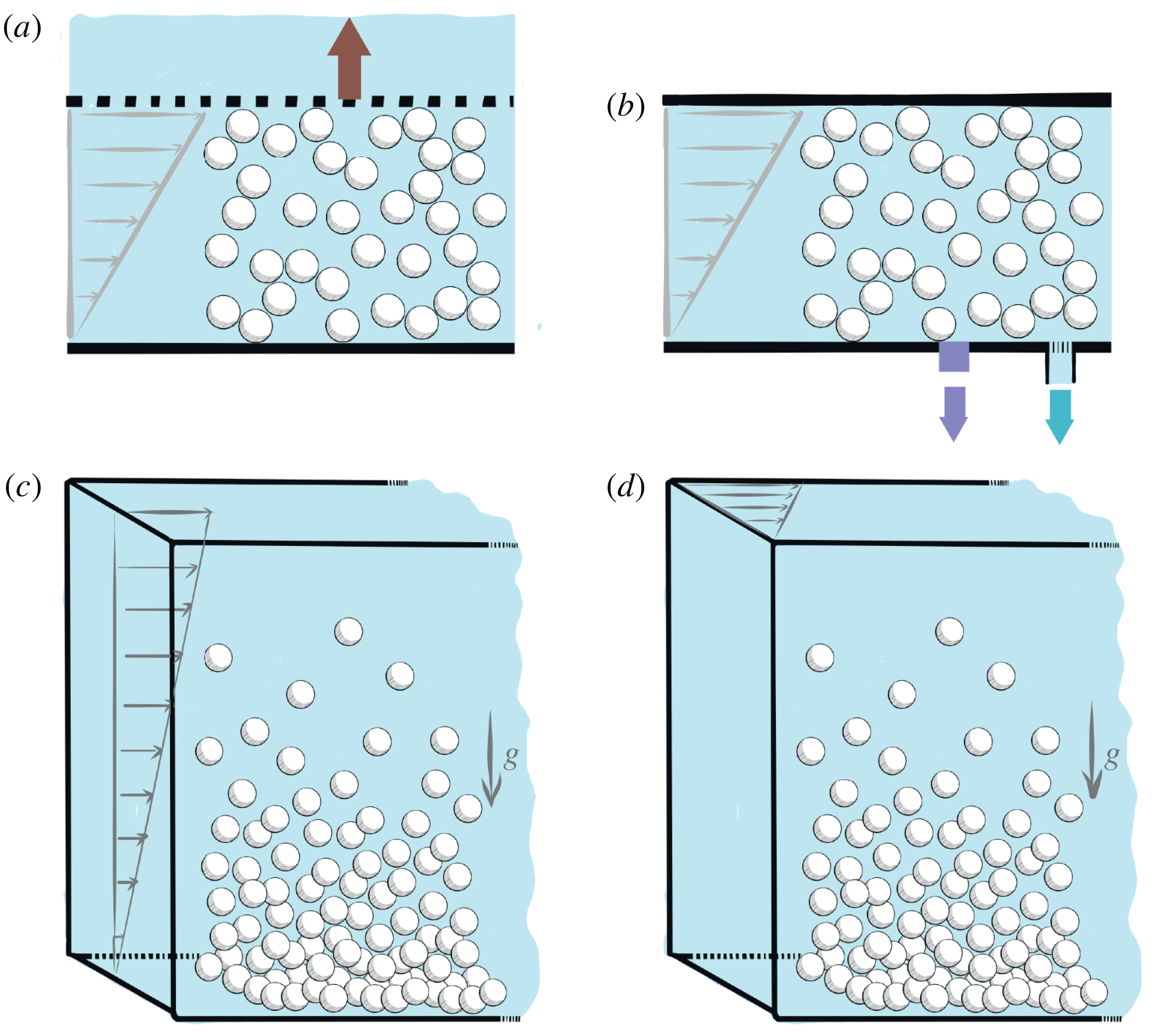
Quantitative measurements of the particle pressure, or more generally of particle normal stresses, are not easily performed, in large part because it is difficult to differentiate between the particle and the fluid pressures as explained above. Conventional rheometers measure the total force exerted by the suspension and thus need to be adapted to measure either the force coming from the particles or that from the fluid (see figure 11). A first direct method consists in using a grid as a top plate which enables fluid flow through it but not particles owing to mesh openings smaller than the particle sizes, as done in an annular shearing cell by Boyer et al. (Reference Boyer, Guazzelli and Pouliquen2011a ) (see figure 11 a). Measuring the forces exerted on the grid thus gives access to the pressure exerted by the particles (while the grid pressure coincides with the particle pressure for dense suspensions, this may not be completely true otherwise, as we shall see later). An alternative method is to measure the fluid pressure and infer the particle pressure by subtraction from the total pressure as done by Dbouk et al. (Reference Dbouk, Lobry and Lemaire2013) in a parallel-plate rheometer and by Garland et al. (Reference Garland, Gauthier, Martin and Morris2013) in a Couette rheometer (see figure 11 b). This can be achieved by measuring the pore pressure behind a hole covered by a grid in a tube filled with the suspending fluid as done in the analogous osmotic pressure experiment described in the preceding paragraph (Deboeuf et al. Reference Deboeuf, Gauthier, Martin, Yurkovetsky and Morris2009). A second pressure sensor measures the total pressure exerted by the suspension, and the difference between the two measurements provides an estimation of the particle pressure.

Other configurations, such as viscous resuspension of an initially settled layer of negatively buoyant spheres, also provide indirect information on the particle pressure (see figure 11 c,d). Measurements can be conducted in the plane of shear using an annular parallel geometry (Leighton & Acrivos Reference Leighton and Acrivos1986) or in the plane perpendicular to the plane of shear (i.e. in the vorticity direction) using a Couette device (Acrivos, Mauri & Fan Reference Acrivos, Mauri and Fan1993). When the suspension is sheared, particle normal stresses develop, leading to a dilatation of the sediment layer. An equilibrium resuspension height is reached when the gravity force which pulls the particles downwards is balanced by the divergence of the particle normal stresses which tends to dilate the sediment. Viscous resuspension will be treated in more detail in § 3.3.2. Along the same lines, shear-induced migration that we introduce in figure 8(a) can also give some indirect information on particle normal stresses, as the divergence of the normal stresses becomes zero when the flow is fully developed. This migration phenomenon will be addressed more fully in § 3.3.1.

Using the same dimensional arguments as those used in § 2 for the viscosity and the normal-stress differences, particle normal stresses are also found to scale viscously and are linear in the modulus of the shear rate, since they must be independent of the sign of the shear rate as previously noted for the normal stresses of the whole suspension. As suggested by the physical discussions of the previous paragraphs of this section, particle pressures are positive, meaning that normal stresses are negative. The particle normal stress along the direction perpendicular to the shearing flow direction can thus be written as $-\unicode[STIX]{x1D70E}_{22}^{p}=\unicode[STIX]{x1D702}_{n,2}\unicode[STIX]{x1D702}_{f}|\dot{\unicode[STIX]{x1D6FE}}|$ . We introduce here a so-called relative normal viscosity, $\unicode[STIX]{x1D702}_{n,2}(\unicode[STIX]{x1D719})$ , which again is solely a function of $\unicode[STIX]{x1D719}$ and presents the same divergence with $\unicode[STIX]{x1D719}$ as $\unicode[STIX]{x1D702}_{s}(\unicode[STIX]{x1D719})$ when approaching the critical volume fraction $\unicode[STIX]{x1D719}_{c}$ , i.e. $\unicode[STIX]{x1D702}_{s}$ and $\unicode[STIX]{x1D702}_{n,2}$ both diverge as ${\sim}(\unicode[STIX]{x1D719}_{c}-\unicode[STIX]{x1D719})^{-2}$ at jamming. Note that, for the moment, only the normal-stress component along the flow-gradient direction is discussed; the other components are discussed in the following.

Figure 12.

Ratio of particle pressure in the gradient direction to shear stress, $-\unicode[STIX]{x1D70E}_{22}^{p}/\unicode[STIX]{x1D70F}=\unicode[STIX]{x1D702}_{n,2}/\unicode[STIX]{x1D702}_{s}=1/\unicode[STIX]{x1D707}$ , versus $\unicode[STIX]{x1D719}$ . Experiments: of Boyer et al. (Reference Boyer, Guazzelli and Pouliquen2011a ) with PS spheres of diameter $d=580~\unicode[STIX]{x03BC}\text{m}$ suspended in polyethylene glycol-ran-propylene glycol monobutyl ether as well as PMMA spheres of diameter $d=1100~\unicode[STIX]{x03BC}\text{m}$ suspended in a Triton X-100/water/zinc chloride mixture; of Dagois-Bohy et al. (Reference Dagois-Bohy, Hormozi, Guazzelli and Pouliquen2015) with PS spheres of similar sizes, both measuring the pressure on a grid; of Dbouk et al. (Reference Dbouk, Lobry and Lemaire2013) with PS spheres of diameter $d=140~\unicode[STIX]{x03BC}\text{m}$ suspended in a mixture of water, UCON oil and zinc bromide; and of Garland et al. (Reference Garland, Gauthier, Martin and Morris2013) with PS spheres of diameters $d=40$ and $140~\unicode[STIX]{x03BC}\text{m}$ suspended in polyethylene glycol-ran-propylene glycol monobutyl ether, both combining measurements of pore pressure and total pressure. Correlation: of Zarraga et al. (Reference Zarraga, Hill and Leighton2000),  $2.17\unicode[STIX]{x1D719}^{3}\exp (2.34\unicode[STIX]{x1D719})$ , using the resuspension data of Acrivos et al. (Reference Acrivos, Mauri and Fan1993) to infer $\unicode[STIX]{x1D70E}_{33}^{p}$ and their measurement of the second normal-stress difference, $N_{2}=\unicode[STIX]{x1D6F4}_{22}-\unicode[STIX]{x1D6F4}_{33}$ , of the whole suspension mixture (assuming that the differences in normal stresses of the whole suspension and of the particle phase are identical). Numerical simulations: of Gallier et al. (Reference Gallier, Lemaire, Peters and Lobry2014) containing only the contact contributions for $\unicode[STIX]{x1D70E}_{22}^{p}$ with $\unicode[STIX]{x1D707}_{p}=0.5$ . Rheological models: that proposed by Morris & Boulay (Reference Morris and Boulay1999),  $\unicode[STIX]{x1D702}_{s}(\unicode[STIX]{x1D719})=1+(5/2)\unicode[STIX]{x1D719}(1-\unicode[STIX]{x1D719}/\unicode[STIX]{x1D719}_{c})^{-1}+K_{s}(\unicode[STIX]{x1D719}/\unicode[STIX]{x1D719}_{c})^{2}(1-\unicode[STIX]{x1D719}/\unicode[STIX]{x1D719}_{c})^{-2}$ and $\unicode[STIX]{x1D702}_{n}(\unicode[STIX]{x1D719})=K_{n}(\unicode[STIX]{x1D719}/\unicode[STIX]{x1D719}_{c})^{2}(1-\unicode[STIX]{x1D719}/\unicode[STIX]{x1D719}_{c})^{-2}$ with $K_{s}\simeq 0.1$ , $K_{n}\simeq 0.75$ , $\unicode[STIX]{x1D706}_{2}\simeq 0.8$ and $\unicode[STIX]{x1D706}_{3}\simeq 0.5$ ; and that proposed by Boyer et al. (Reference Boyer, Guazzelli and Pouliquen2011a ),  $\unicode[STIX]{x1D702}_{s}(\unicode[STIX]{x1D719})=1+(5/2)\unicode[STIX]{x1D719}(1-\unicode[STIX]{x1D719}/\unicode[STIX]{x1D719}_{c})^{-1}+\unicode[STIX]{x1D707}^{c}(\unicode[STIX]{x1D719})(\unicode[STIX]{x1D719}/\unicode[STIX]{x1D719}_{c})^{2}(1-\unicode[STIX]{x1D719}/\unicode[STIX]{x1D719}_{c})^{-2}$ and $\unicode[STIX]{x1D702}_{n}(\unicode[STIX]{x1D719})=(\unicode[STIX]{x1D719}/\unicode[STIX]{x1D719}_{c})^{2}(1-\unicode[STIX]{x1D719}/\unicode[STIX]{x1D719}_{c})^{-2}$ with $\unicode[STIX]{x1D707}^{c}(\unicode[STIX]{x1D719})=\unicode[STIX]{x1D707}_{1}+(\unicode[STIX]{x1D707}_{2}-\unicode[STIX]{x1D707}_{1})/[1+I_{0}\unicode[STIX]{x1D719}^{2}(\unicode[STIX]{x1D719}_{c}-\unicode[STIX]{x1D719})^{-2}]$ and $\unicode[STIX]{x1D707}_{1}\simeq 0.32,~\unicode[STIX]{x1D707}_{2}\simeq 0.7,~I_{0}\simeq 0.005$ , $\unicode[STIX]{x1D706}_{2}\simeq 0.95$ and $\unicode[STIX]{x1D706}_{3}\simeq 0.6$ . In both cases, we have plotted $\unicode[STIX]{x1D702}_{n,2}/\unicode[STIX]{x1D702}_{s}=\unicode[STIX]{x1D706}_{2}\unicode[STIX]{x1D702}_{n}/\unicode[STIX]{x1D702}_{s}$ and have chosen $\unicode[STIX]{x1D719}_{c}=0.585$ as found experimentally by Boyer et al. (Reference Boyer, Guazzelli and Pouliquen2011a ) but have also plotted the correlation of Morris & Boulay (Reference Morris and Boulay1999) with their originally chosen $\unicode[STIX]{x1D719}_{c}=0.68$ .

Figure 12 shows a collection of most of the available experimental data obtained by using the methods presented earlier and sketched in figure 11. As for the normal-stress differences of the whole suspension presented in § 2.2, we have plotted the ratio of particle pressure to shear stress, $-\unicode[STIX]{x1D70E}_{22}^{p}/\unicode[STIX]{x1D70F}$ . This ratio is also that of the normal and shear viscosities and is related to an effective friction coefficient, $\unicode[STIX]{x1D707}$ , as $-\unicode[STIX]{x1D70E}_{22}^{p}/\unicode[STIX]{x1D70F}=\unicode[STIX]{x1D702}_{n,2}/\unicode[STIX]{x1D702}_{s}=1/\unicode[STIX]{x1D707}$ (the frictional approach to suspension rheology will be further discussed in § 4.1). It is important to emphasise that $\unicode[STIX]{x1D707}$ is a ‘macroscopic’ effective friction coefficient of the suspension and thus differs from the ‘microscopic’ friction coefficient between particles, $\unicode[STIX]{x1D707}_{p}$ , introduced earlier in § 2.1. Despite some scatter, the data coming from different methods and using different fluid–particle combinations show a reasonable collapse onto the same curve (with the exception of the correlation of Zarraga et al. (Reference Zarraga, Hill and Leighton2000), which presents deviations at large $\unicode[STIX]{x1D719}$ ). Importantly, the ratio $\unicode[STIX]{x1D702}_{n,2}/\unicode[STIX]{x1D702}_{s}$ tends towards a constant value ( ${\approx}3$ , i.e. $\unicode[STIX]{x1D707}_{c}\approx 0.3$ ) when $\unicode[STIX]{x1D719}$ reaches $\unicode[STIX]{x1D719}_{c}({\approx}0.58{-}0.59)$ , implying that the divergences of the two viscosities are similar. In the dilute limit, this ratio is seen to vanish, meaning that $\unicode[STIX]{x1D702}_{n,2}$ also vanishes since $\unicode[STIX]{x1D702}_{s}$ stays finite ( $\unicode[STIX]{x1D702}_{s}=1$ at $\unicode[STIX]{x1D719}=0$ ). Whether there exists a critical volume fraction below which the particle pressure disappears remains an open question. We have also reported in figure 12 the contact contributions to the normal stress coming from the simulations of Gallier et al. (Reference Gallier, Lemaire, Peters and Lobry2014) presented earlier for the viscosity and normal-stress differences in § 2 (see figures 4 and 7). These simulations, which account for particle roughness and frictional contacts between the particles, agree well with the experiments. This suggests that contact may act as the dominant component in the particle pressure in particular at large $\unicode[STIX]{x1D719}$ (this will be discussed further in § 5.2).

Up to now, only the component of the particle stress along the gradient direction, i.e. $-\unicode[STIX]{x1D70E}_{22}^{p}$ , has been addressed. In some configurations, it is also possible to measure the other components, $-\unicode[STIX]{x1D70E}_{11}^{p}$ and $-\unicode[STIX]{x1D70E}_{33}^{p}$ , and to show that differences in particle normal stresses exist. However, experimental data are scarce and often rely on measurements of the differences in normal stresses of the bulk suspension presented in § 2.2. This is, for instance, the case for the different components given by Zarraga et al. (Reference Zarraga, Hill and Leighton2000), who use the resuspension data of Acrivos et al. (Reference Acrivos, Mauri and Fan1993) to infer $\unicode[STIX]{x1D70E}_{33}^{p}$ and their measurement of $N_{1}$ and $N_{2}$ (see figure 7), as well as for those given by Dbouk et al. (Reference Dbouk, Lobry and Lemaire2013), who use their measurement of $\unicode[STIX]{x1D70E}_{22}^{p}$ (see figure 12) and of $N_{1}$ and $N_{2}$ (see figure 7). Whether the differences in normal stresses of the bulk suspension and of the particle phase coincide is not completely deciphered and is a question related to the origin of the stresses that we will try to address in the following § 3.2. In the dense regime, where contacts between the particles are pre-eminent, it is likely that the two may be similar.

The particle normal stresses can be written in a tensorial form as

(3.1) $$\begin{eqnarray}-\unicode[STIX]{x1D702}_{f}|\dot{\unicode[STIX]{x1D6FE}}|\left(\begin{array}{@{}ccc@{}}\unicode[STIX]{x1D702}_{n,1}(\unicode[STIX]{x1D719}) & 0 & 0\\ 0 & \unicode[STIX]{x1D702}_{n,2}(\unicode[STIX]{x1D719}) & 0\\ 0 & 0 & \unicode[STIX]{x1D702}_{n,3}(\unicode[STIX]{x1D719})\end{array}\right),\end{eqnarray}$$

where the normal viscosities in each direction, $\unicode[STIX]{x1D702}_{n,i}(\unicode[STIX]{x1D719})$ (with $i=1$ , 2 and 3), tend towards zero in the dilute limit and diverge in a similar way as $\unicode[STIX]{x1D702}_{s}(\unicode[STIX]{x1D719})$ when approaching $\unicode[STIX]{x1D719}_{c}$ . While having similar high- and low-concentration limits, the different components of the particle normal stress may not vary in exactly the same way with $\unicode[STIX]{x1D719}$ (Dbouk et al. Reference Dbouk, Lobry and Lemaire2013). However, there are not enough observations to yield firm conclusions on their respective behaviours. In the literature, a simplified form of this particle normal-stress tensor has often been used, assuming a similar $\unicode[STIX]{x1D719}$ dependence in all directions (Morris & Boulay Reference Morris and Boulay1999). The particle normal-stress tensor (3.1) then takes the simpler form

(3.2) $$\begin{eqnarray}-\unicode[STIX]{x1D702}_{n}(\unicode[STIX]{x1D719})\unicode[STIX]{x1D702}_{f}|\dot{\unicode[STIX]{x1D6FE}}|\left(\begin{array}{@{}ccc@{}}1 & 0 & 0\\ 0 & \unicode[STIX]{x1D706}_{2} & 0\\ 0 & 0 & \unicode[STIX]{x1D706}_{3}\end{array}\right),\end{eqnarray}$$

with

(3.3) $$\begin{eqnarray}\unicode[STIX]{x1D702}_{n}(\unicode[STIX]{x1D719})=K_{n}\frac{\unicode[STIX]{x1D719}^{2}}{(\unicode[STIX]{x1D719}_{c}-\unicode[STIX]{x1D719})^{2}},\end{eqnarray}$$

which gives an $O(\unicode[STIX]{x1D719}^{2})$ dependence at small $\unicode[STIX]{x1D719}$ and a divergence in $(\unicode[STIX]{x1D719}_{c}-\unicode[STIX]{x1D719})^{-2}$ similar to that of $\unicode[STIX]{x1D702}_{s}$ near $\unicode[STIX]{x1D719}_{c}$ . This is a practically useful simplification as the particle normal-stress tensor is only determined by a single scalar function, $\unicode[STIX]{x1D702}_{n}(\unicode[STIX]{x1D719})$ , and two constant anisotropy coefficients, $\unicode[STIX]{x1D706}_{2}$ and $\unicode[STIX]{x1D706}_{3}$ , and thus is amenable to computation, e.g. for shear-induced migration or resuspension calculations, as will be seen in § 3.3. The coefficients were found to be $K_{n}\approx 0.75$ , $\unicode[STIX]{x1D706}_{2}\approx 0.8$ and $\unicode[STIX]{x1D706}_{3}\approx 0.5$ by Morris & Boulay (Reference Morris and Boulay1999), who chose them to match experimental results on shear-induced migration, and $K_{n}\approx 1$ , $\unicode[STIX]{x1D706}_{2}\approx 0.95$ and $\unicode[STIX]{x1D706}_{3}\approx 0.6$ by Boyer et al. (Reference Boyer, Guazzelli and Pouliquen2011a ) and Couturier et al. (Reference Couturier, Boyer, Pouliquen and Guazzelli2011), who inferred them from pressure-imposed rheological and normal-stress difference measurements. The correlations proposed by Morris & Boulay (Reference Morris and Boulay1999) as well as Boyer et al. (Reference Boyer, Guazzelli and Pouliquen2011a ) and Couturier et al. (Reference Couturier, Boyer, Pouliquen and Guazzelli2011) are reported in figure 12 with $\unicode[STIX]{x1D719}_{c}=0.585$ . The equations used for $\unicode[STIX]{x1D702}_{s}$ are similar to that of Eilers that we gave at the end of § 2.1. While a quantitative difference is observed at high concentrations, in particular for the values at $\unicode[STIX]{x1D719}_{c}$ as $1/\unicode[STIX]{x1D707}(\unicode[STIX]{x1D719}_{c})=\unicode[STIX]{x1D706}_{2}/\unicode[STIX]{x1D707}_{1}\approx 2.97$ in the Boyer et al. (Reference Boyer, Guazzelli and Pouliquen2011a ) rheology while $1/\unicode[STIX]{x1D707}(\unicode[STIX]{x1D719}_{c})=\unicode[STIX]{x1D706}_{2}K_{n}/K_{s}\approx 6$ in the Morris & Boulay (Reference Morris and Boulay1999) rheology, similar trends are observed over the lower range of $\unicode[STIX]{x1D719}$ . Note that Morris & Boulay (Reference Morris and Boulay1999) originally used $\unicode[STIX]{x1D719}_{c}=0.68$ ; this original correlation is also plotted in figure 12.

3.2 Two-phase modelling of viscous suspensions

In principle, a complete calculation of the motion of solid particles in a Newtonian fluid is given by solving Newton’s equations of motion for the translation and the rotation of each particle and the Navier–Stokes equations, or the Stokes equation in the absence of inertia, for the fluid with no-slip conditions on the surface of each particle and on the walls. Such type of direct calculation can now be done numerically, as we have seen in the above sections, although this may prove to be quite a complex task. An alternative route is to use continuum two-phase modelling, which assumes that the interstitial fluid and the particles are two intertwined continuous phases, and to derive the governing equations that describe the system in an average sense for each phase. This has important practical interest as it provides the knowledge of average quantities, e.g. the average values of the fluid velocity, particle velocity and fluid pressure over some small region surrounding each point of the system of interest, which is all that may be required in most of the flow situations. Different ways of performing the averaging process have been used: (i) local space averaging over regions smaller than the macroscopic length scale but larger than the particle size or (ii) ensemble averaging at each point of space over ‘macroscopically equivalent’ systems. Each type of averaging is purely a formal process and should lead to essentially the same equations if properly done. It generates a greater number of averaged quantities than there are available equations and therefore there is a closure problem, i.e. a need for some constitutive relations, which is a central issue in the modelling.

We do not provide here the details of the formal derivation of the governing equations but give some hints on how to proceed. For this purpose, we follow Jackson (Reference Jackson1997) by using local space averages which are closer to the way quantities are measured experimentally. The basic idea behind this approach is to replace the point variables by local mean variables by averaging the point variables over a representative region that contains enough particles but is still smaller than the length scale of macroscopic spatial gradients. The formal averaging process is performed using a weighting function having a radius of precisely the size of the representative region so that the obtained volume average of a property is the reflection of its value only in the vicinity of a given location, $\boldsymbol{x}$ . Considering a suspension of non-colloidal rigid spheres of density $\unicode[STIX]{x1D70C}_{p}$ suspended in a Newtonian fluid of density $\unicode[STIX]{x1D70C}_{f}$ and viscosity $\unicode[STIX]{x1D702}_{f}$ , we can then define at each point, $\boldsymbol{x}$ , the volume fraction of the solid and fluid phase, $\unicode[STIX]{x1D719}$ and $1-\unicode[STIX]{x1D719}$ , respectively, and the local mean particle and fluid velocity, $\boldsymbol{u}^{p}$ and $\boldsymbol{u}^{f}$ , respectively. We can also derive the stresses of each phase and the interphase force. As in any continuum treatment, the forces are divided into body forces and surface forces and this needs to be done in a way that reflects the fact that the particles are dispersed in the fluid phase.

Considering the interphase force first, the way to proceed to obtain the quantity of interest for a dispersed mixture of particles is (i) to integrate the fluid stress on the boundary of a particle to obtain the force exerted by the fluid on a particle, $\boldsymbol{f}^{h}$ (i.e. the zeroth moment of the fluid traction about the particle centre), and then (ii) to average over all the particles present in the same representative volume to obtain the net fluid force acting through the centre of mass of this assembly of particles, $n\langle \,\boldsymbol{f}^{h}\rangle ^{p}$ , where $n$ is the particle number density (number of particles per unit volume). The hydrodynamic force on the particle phase is thus a particle-averaged force as is intuitively reasonable for a dispersed mixture. Because of the partition into body and surface forces already mentioned above, the effective continuum stresses of the two phases cannot involve this hydrodynamic force any more. The effective stress of the particulate phase, $\unicode[STIX]{x1D748}^{pp}$ , is found to comprise solely of terms coming from non-hydrodynamic interparticle (contact) interactions (i.e. the particle-averaged first moment of the contact traction and higher-order terms), while that of the fluid phase contains the mean fluid stress tensor, $(1-\unicode[STIX]{x1D719})\langle \unicode[STIX]{x1D748}\rangle ^{f}$ , but is also augmented by terms coming from fluid–particle interactions (i.e. the particle-averaged first moment of the fluid traction and higher-order terms), $\unicode[STIX]{x1D748}^{fp}$ . Further details of the derivation can be found in Jackson (Reference Jackson1997) and Nott, Guazzelli & Pouliquen (Reference Nott, Guazzelli and Pouliquen2011). We give below the obtained governing averaged equations.

The equations of continuity for the fluid and the particles are, respectively,

(3.4) $$\begin{eqnarray}\displaystyle & \displaystyle \frac{\unicode[STIX]{x2202}(1-\unicode[STIX]{x1D719})}{\unicode[STIX]{x2202}t}+\unicode[STIX]{x1D735}\boldsymbol{\cdot }[(1-\unicode[STIX]{x1D719})\boldsymbol{u}^{f}]=0, & \displaystyle\end{eqnarray}$$

(3.5) $$\begin{eqnarray}\displaystyle & \displaystyle \frac{\unicode[STIX]{x2202}\unicode[STIX]{x1D719}}{\unicode[STIX]{x2202}t}+\unicode[STIX]{x1D735}\boldsymbol{\cdot }(\unicode[STIX]{x1D719}\boldsymbol{u}^{p})=0. & \displaystyle\end{eqnarray}$$

Adding (3.4) and (3.5), the suspension, i.e. the mixture of fluid and particles, is found to be incompressible as previously noted,

(3.6) $$\begin{eqnarray}\unicode[STIX]{x1D735}\boldsymbol{\cdot }\boldsymbol{U}=0,\end{eqnarray}$$

where $\boldsymbol{U}=\unicode[STIX]{x1D719}\boldsymbol{u}^{p}+(1-\unicode[STIX]{x1D719})\boldsymbol{u}^{f}$ is the volume-averaged velocity.

In the absence of inertia, the momentum equations for the fluid and particle phases are found to be, respectively,

(3.7) $$\begin{eqnarray}\displaystyle & \displaystyle \unicode[STIX]{x1D735}\boldsymbol{\cdot }[(1-\unicode[STIX]{x1D719})\langle \unicode[STIX]{x1D748}\rangle ^{f}+\unicode[STIX]{x1D748}^{fp}]-n\langle \,\boldsymbol{f}^{h}\rangle ^{p}+\unicode[STIX]{x1D70C}_{f}(1-\unicode[STIX]{x1D719})\boldsymbol{g}=0, & \displaystyle\end{eqnarray}$$

(3.8) $$\begin{eqnarray}\displaystyle & \displaystyle \unicode[STIX]{x1D735}\boldsymbol{\cdot }\unicode[STIX]{x1D748}^{pp}+n\langle \,\boldsymbol{f}^{h}\rangle ^{p}+\unicode[STIX]{x1D70C}_{p}\unicode[STIX]{x1D719}\boldsymbol{g}=0, & \displaystyle\end{eqnarray}$$

where $\boldsymbol{g}$ is the specific gravity force vector. Comparing (3.7) and (3.8), the interphase force is seen to appear in the same form but with opposite signs. If the fluid is Newtonian, the mean fluid stress tensor can be written as $(1-\unicode[STIX]{x1D719})\langle \unicode[STIX]{x1D748}\rangle ^{f}=-(1-\unicode[STIX]{x1D719})p^{\,f}\unicode[STIX]{x1D644}+2\unicode[STIX]{x1D702}_{f}\unicode[STIX]{x1D640}$ , where $p^{\,f}$ is the mean fluid pressure, $\unicode[STIX]{x1D640}$ is the mean strain rate of the whole suspension and $\unicode[STIX]{x1D644}$ is the identity tensor. Adding (3.7) and (3.8) yields the momentum equation for the suspension as a whole, i.e. for the mixture,

(3.9) $$\begin{eqnarray}\unicode[STIX]{x1D735}\boldsymbol{\cdot }[-(1-\unicode[STIX]{x1D719})p^{\,f}\unicode[STIX]{x1D644}+2\unicode[STIX]{x1D702}_{f}\unicode[STIX]{x1D640}+\unicode[STIX]{x1D748}^{fp}+\unicode[STIX]{x1D748}^{pp}]+[\unicode[STIX]{x1D70C}_{f}(1-\unicode[STIX]{x1D719})+\unicode[STIX]{x1D70C}_{p}\unicode[STIX]{x1D719}]\boldsymbol{g},\end{eqnarray}$$

which is simply the balance between gravity and the divergence of the stress tensor of the whole suspension mixture. This total stress tensor can be written as

(3.10) $$\begin{eqnarray}\unicode[STIX]{x1D72E}=-(1-\unicode[STIX]{x1D719})p^{\,f}\unicode[STIX]{x1D644}+2\unicode[STIX]{x1D702}_{f}\unicode[STIX]{x1D640}+\unicode[STIX]{x1D72E}^{(p)},\end{eqnarray}$$

where the first term is a purely isotropic contribution, the second term is the deviatoric stress that would be present in the absence of particles, and the third corresponds to the particle contribution to the whole suspension stress, $\unicode[STIX]{x1D72E}^{(p)}=\unicode[STIX]{x1D748}^{fp}+\unicode[STIX]{x1D748}^{pp}$ , which arises from moments of the whole (fluid and contact) traction. This latter contribution corresponds to the ‘particle stress’ defined by Batchelor (Reference Batchelor1970) for the bulk stress of a suspension. Note that the particle contribution in Batchelor (Reference Batchelor1970) just encompasses the first moment called the ‘stresslet’ while in the present approach $\unicode[STIX]{x1D72E}^{(p)}$ includes higher-order terms to account for a non-uniform suspension state. However, as noted before, the ‘particle-phase stress’ contains only the interparticle (contact) portion, $\unicode[STIX]{x1D748}^{pp}$ , whereas the ‘fluid phase stress’ comprises the hydrodynamic portion,  $\unicode[STIX]{x1D748}^{fp}$ .

The averaged equations have been written for the two phases and for the whole suspension but only two sets are really needed. In the particulate flow community, one commonly uses the equations for the two phases; while in the suspension community, one favours the equations for the whole suspension seen as a continuum as presented in § 2 and complements them by those for one phase when two-phase modelling is needed as described in § 3. This latter description, which uses the averaged equations for the suspension, (3.6) and (3.9), supplemented by those for the particle phase, (3.5) and (3.8), has been developed, in particular, to describe the phenomenon of shear-induced migration introduced in figure 8(a), which will be considered in § 3.3.1. However, at this stage, the averaged momentum balances are formal equations, and do not form a closed set of equations together with the continuity equations. The closure problem requires constitutive laws giving expressions for the interphase force and for the stresses of the bulk suspension and particle phase in terms of the local averaged variables and their derivatives.

The interphase hydrodynamic force contains not only the buoyancy force and the interphase drag, but also a non-drag part (Lhuillier Reference Lhuillier2009; Nott et al. Reference Nott, Guazzelli and Pouliquen2011), thus

(3.11) $$\begin{eqnarray}n\langle \,\boldsymbol{f}^{h}\rangle ^{p}=-\unicode[STIX]{x1D70C}_{f}\unicode[STIX]{x1D719}\boldsymbol{g}+\langle \,\boldsymbol{f}^{h}\rangle _{drag}^{p}+n\langle \,\boldsymbol{f}^{h}\rangle _{non\text{-}drag}^{p}.\end{eqnarray}$$

The interphase drag can generally be approximated by a drag force proportional to the relative velocity between the phases, which can be written for spherical particles of diameter $d$ as

(3.12) $$\begin{eqnarray}n\langle \,\boldsymbol{f}^{h}\rangle _{drag}^{p}=-\frac{18\unicode[STIX]{x1D702}_{f}}{d^{2}}\frac{\unicode[STIX]{x1D719}}{f(\unicode[STIX]{x1D719})}(\boldsymbol{u}^{p}-\boldsymbol{U}),\end{eqnarray}$$

where one can use the empirical hindered settling function

(3.13) $$\begin{eqnarray}f(\unicode[STIX]{x1D719})=(1-\unicode[STIX]{x1D719})^{n_{v}}\end{eqnarray}$$

(with $n_{v}\simeq 5$ at low Reynolds numbers) proposed by Richardson & Zaki (Reference Richardson and Zaki1954). The non-drag portion is more difficult to capture. It is related to forces acting on the particles and involving gradients in the velocity field (Jackson Reference Jackson1997; Lhuillier Reference Lhuillier2009). An attempt at a rigorous derivation by Nott et al. (Reference Nott, Guazzelli and Pouliquen2011) has shown that this non-drag portion can be written as the divergence of a hydrodynamic stress, $\unicode[STIX]{x1D748}^{hp}$ . This stress has been found to be related to the moments of the interphase force taken at the midpoint between particles. It differs from the particle contribution to the hydrodynamic part of the whole suspension stress, $\unicode[STIX]{x1D748}^{fp}$ , which is related to the moments of the fluid traction on the surface of the particles about their centres.

We can then revisit the particle-phase momentum equation (3.8) and rewrite it as

(3.14) $$\begin{eqnarray}\unicode[STIX]{x1D735}\boldsymbol{\cdot }\unicode[STIX]{x1D748}^{p}+n\langle \,\boldsymbol{f}^{h}\rangle _{drag}^{p}+(\unicode[STIX]{x1D70C}_{p}-\unicode[STIX]{x1D70C}_{f})\unicode[STIX]{x1D719}\boldsymbol{g}=0,\end{eqnarray}$$

where the stress of the particle phase, $\unicode[STIX]{x1D748}^{p}=\unicode[STIX]{x1D748}^{pp}+\unicode[STIX]{x1D748}^{hp}$ , comprises an interparticle contact stress, $\unicode[STIX]{x1D748}^{pp}$ , and a hydrodynamic stress, $\unicode[STIX]{x1D748}^{hp}$ , coming from the non-drag portion of the interphase force. This stress can be inferred from the measurements and proposed expressions discussed in § 3.1. However, as noted earlier, it is unclear whether these measurements completely capture $\unicode[STIX]{x1D748}^{p}$ . For instance, the pressure grid measurement may only capture the contact portion, $\unicode[STIX]{x1D748}^{pp}$ , and it is also unclear whether the pore pressure measurements can seize the hydrodynamic portion, $\unicode[STIX]{x1D748}^{hp}$ . However, we expect that, at large $\unicode[STIX]{x1D719}$ , $\unicode[STIX]{x1D748}^{pp}$ may be the dominant portion as suggested by the comparison with the numerical simulations of Gallier et al. (Reference Gallier, Lemaire, Peters and Lobry2014) reporting only the contact contribution in figure 12. Along the same lines, the proposed expression (3.3) for the normal viscosity may not be valid for the whole range of $\unicode[STIX]{x1D719}$ and may only be realistic for large  $\unicode[STIX]{x1D719}$ .

Lastly, we come back to the suspension momentum equation (3.9). The measurements and proposed correlations discussed in § 2 provide some information on the stress tensor of the whole suspension, $\unicode[STIX]{x1D72E}$ (in particular on the shear viscosity, $\unicode[STIX]{x1D702}_{s}(\unicode[STIX]{x1D719})$ , and normal-stress differences, $N_{1}$ and $N_{2}$ ), but there are still some uncertainties and we do not yet possess a full tensorial form.

3.3 Two-phase flows of suspensions

3.3.1 Shear-induced migration

This phenomenon was first clearly identified in a Couette rheometer, such as that shown in figure 3(c), where the particles were seen to migrate from the high-shear-rate region in the gap to the low-shear-rate region in the cavity beneath the inner cylinder (Gadala-Maria Reference Gadala-Maria1979; Leighton & Acrivos Reference Leighton and Acrivos1987) and motivated a large body of research due to its implication for the characterisation of suspension rheology. In pressure-driven Poiseuille flow, the particles are seen to migrate towards the centreline, as illustrated in figure 8(a). Again, since the first observation of such suspension inhomogeneities in pipe flows by Karnis, Goldsmith & Mason (Reference Karnis, Goldsmith and Mason1966) and in channel flows by Koh, Hookham & Leal (Reference Koh, Hookham and Leal1994), several experimental studies have been performed to measure migration in pressure-driven flow in a pipe or a channel. Earlier simulations of the pressure-driven flow in a two-dimensional channel of a suspension were conducted using Stokesian dynamics (Nott & Brady Reference Nott and Brady1994). The important output of these simulations was to show that the phenomenon was not due to inertial effects since Stokesian dynamics imposed a zero Reynolds number. More recent methods, such as the force coupling method of Yeo & Maxey (Reference Yeo and Maxey2011) wherein the flow disturbance induced by each particle is represented by a low-order multipole expansion, are now also providing effective information on the migration process.

Since the first observation of shear-induced migration, two types of migration models have been proposed. Early efforts used a diffusion model, in which the particle migration flux was expressed in terms of the gradients of the particle concentration and shear rate. This diffusion model is successful in predicting migration in wide-gap Couette and pressure-driven Poiseuille flows, but fails to predict the absence of migration in curvilinear torsional flows (Morris & Boulay Reference Morris and Boulay1999). A more recent and rather successful model, termed the suspension balance model, relates the migration flux to the divergence of the normal stress of the particle phase (Nott & Brady Reference Nott and Brady1994; Morris & Boulay Reference Morris and Boulay1999; Lhuillier Reference Lhuillier2009; Nott et al. Reference Nott, Guazzelli and Pouliquen2011) and uses the two-phase approach described in § 3.2. We will now use this two-phase modelling to give some indication of the physical mechanisms involved and its connection to the suspension rheology.

To derive the migration equation, we combine the continuity equation for the particles (3.5) with the incompressibility of the suspension (3.6),

(3.15) $$\begin{eqnarray}\frac{\unicode[STIX]{x2202}\unicode[STIX]{x1D719}}{\unicode[STIX]{x2202}t}+\boldsymbol{U}\boldsymbol{\cdot }\unicode[STIX]{x1D735}\unicode[STIX]{x1D719}=-\unicode[STIX]{x1D735}\boldsymbol{\cdot }\unicode[STIX]{x1D719}(\boldsymbol{u}^{p}-\boldsymbol{U}),\end{eqnarray}$$

to exhibit the migration flux $\unicode[STIX]{x1D719}(\boldsymbol{u}^{p}-\boldsymbol{U})$ . For neutrally buoyant particles ( $\unicode[STIX]{x1D70C}=\unicode[STIX]{x1D70C}_{p}=\unicode[STIX]{x1D70C}_{f}$ ), this flux can be inferred from the particle-phase momentum equation (3.14) together with the expression for the drag (3.12),

(3.16) $$\begin{eqnarray}\unicode[STIX]{x1D719}(\boldsymbol{u}^{p}-\boldsymbol{U})=\frac{d^{2}f(\unicode[STIX]{x1D719})}{18\unicode[STIX]{x1D702}_{f}}\unicode[STIX]{x1D735}\boldsymbol{\cdot }\unicode[STIX]{x1D748}^{p}.\end{eqnarray}$$

This modelling thus predicts that particle migration is driven by the divergence of the normal components of the particle-phase stress.

Considering a pressure-driven flow in a two-dimensional channel of width $H$ as a basic example, the migration equation can be written as

(3.17) $$\begin{eqnarray}\displaystyle \frac{\unicode[STIX]{x2202}\unicode[STIX]{x1D719}}{\unicode[STIX]{x2202}t} & = & \displaystyle -\frac{d^{2}}{18\unicode[STIX]{x1D702}_{f}}\frac{\unicode[STIX]{x2202}}{\unicode[STIX]{x2202}x_{2}}\left[f(\unicode[STIX]{x1D719})\frac{\unicode[STIX]{x2202}\unicode[STIX]{x1D70E}_{22}^{p}}{\unicode[STIX]{x2202}x_{2}}\right]\nonumber\\ \displaystyle & = & \displaystyle \frac{d^{2}}{18}\frac{\unicode[STIX]{x2202}}{\unicode[STIX]{x2202}x_{2}}\left\{f(\unicode[STIX]{x1D719})\frac{\unicode[STIX]{x2202}[\unicode[STIX]{x1D702}_{n,2}(\unicode[STIX]{x1D719})\unicode[STIX]{x1D702}_{f}|\dot{\unicode[STIX]{x1D6FE}}|]}{\unicode[STIX]{x2202}x_{2}}\right\},\end{eqnarray}$$

where $x_{2}$ is the flow-gradient axis (note that the above expression assumes $\boldsymbol{U}\boldsymbol{\cdot }\unicode[STIX]{x1D735}\unicode[STIX]{x1D719}\approx 0$ , since the cross-stream migration is much slower than the mean flow dynamics and the volume-averaged velocity $U$ is considered to be mostly along the flow direction $1$ , and not to depend on $x_{1}$ ). To solve the problem, this equation needs to be complemented by the momentum equation for the whole suspension along $x_{1}$ ,

(3.18) $$\begin{eqnarray}-G+\frac{\unicode[STIX]{x2202}[\unicode[STIX]{x1D702}_{s}(\unicode[STIX]{x1D719})\unicode[STIX]{x1D702}_{f}\dot{\unicode[STIX]{x1D6FE}}]}{\unicode[STIX]{x2202}x_{2}}=0,\end{eqnarray}$$

which means that the gradient of shear stress across the channel, $\unicode[STIX]{x1D70F}=\unicode[STIX]{x1D702}_{s}(\unicode[STIX]{x1D719})\unicode[STIX]{x1D702}_{f}\dot{\unicode[STIX]{x1D6FE}}$ , is constant ( $G$ is the pressure gradient along the flow direction, $x_{1}$ ).

When the flow is fully developed, the particle pressure is constant across the channel as

(3.19) $$\begin{eqnarray}-\frac{\unicode[STIX]{x2202}\unicode[STIX]{x1D70E}_{22}^{p}}{\unicode[STIX]{x2202}x_{2}}=\frac{\unicode[STIX]{x2202}[\unicode[STIX]{x1D702}_{n,2}(\unicode[STIX]{x1D719})\unicode[STIX]{x1D702}_{f}|\dot{\unicode[STIX]{x1D6FE}}|]}{\unicode[STIX]{x2202}x_{2}}=0.\end{eqnarray}$$

Since $\dot{\unicode[STIX]{x1D6FE}}$ varies in the gradient direction (zero at the centre and large at the wall), $\unicode[STIX]{x1D702}_{n,2}(\unicode[STIX]{x1D719})$ and thus $\unicode[STIX]{x1D719}$ must also vary to keep $\unicode[STIX]{x1D70E}_{22}^{p}$ constant. Consequently, where the shear rate is low, the concentration is high and vice versa and the particles must have migrated to the centre. To go a little bit further and obtain the concentration variation, we can circumvent singularities arising at the centre of the channel by computing the friction coefficient using equations (3.18) and (3.19),

(3.20) $$\begin{eqnarray}\unicode[STIX]{x1D707}(\unicode[STIX]{x1D719})=\frac{\unicode[STIX]{x1D702}_{s}(\unicode[STIX]{x1D719})}{\unicode[STIX]{x1D702}_{n,2}(\unicode[STIX]{x1D719})}=\unicode[STIX]{x1D707}_{w}|x_{2}|,\end{eqnarray}$$

where $\unicode[STIX]{x1D707}_{w}$ is the friction coefficient at the channel wall (the origin $0$ is taken at the centre of the channel). The volume fraction $\unicode[STIX]{x1D719}$ reaches the maximum packing fraction,  $\unicode[STIX]{x1D719}_{c}$ , in a central region of the channel delimited by $x_{plug}=\pm \unicode[STIX]{x1D707}(\unicode[STIX]{x1D719}_{c})/\unicode[STIX]{x1D707}_{w}$ . Outside of this plugged region, the concentration profile is given by inverting the friction function (3.20) while ensuring that the total volume fraction in the channel corresponds to the initial (uniform) volume fraction $\unicode[STIX]{x1D719}_{0}$ (therefore setting the value of  $\unicode[STIX]{x1D707}_{w}$ ).

Figure 13.

Shear-induced migration in a channel flow. Evolution of the concentration profiles for different confinement, $H/d=11$ in (a,b) and $H/d=20$ in (c,d), and different initial bulk volume fraction, $\unicode[STIX]{x1D719}_{0}$ , from solving the migration equation (3.17) using the rheological laws (with a realistic $\unicode[STIX]{x1D719}_{c}=0.585$ ) of Morris & Boulay (Reference Morris and Boulay1999) (green solid lines) and Boyer et al. (Reference Boyer, Guazzelli and Pouliquen2011a ) (blue dashed lines) at different dimensionless times (made dimensionless by using the channel half width $H/2$ as the length scale and the mean velocity of the channel flow as the velocity scale) $0,10,50,200,500$ (a,b) and $0,10,50,100,1000,2000$ (c,d); thicker lines indicate the steady solutions. Also shown are fully developed concentration profiles from the numerical simulations of Yeo & Maxey (Reference Yeo and Maxey2011) and the experimental measurements of Lyon & Leal (Reference Lyon and Leal1998) at similar values of $H/d$ and $\unicode[STIX]{x1D719}_{0}$ . Comparison is also provided in (b) with the experiments of Snook, Butler & Guazzelli (Reference Snook, Butler and Guazzelli2016) in a pipe flow at a similar value of $D/d=8.21$ , where $D$ is the diameter of the pipe.

To obtain the dynamics of the migration, (3.17) needs to be integrated numerically using the shear rate given by (3.18). There are some difficulties at the centreline of the channel where the shear rate approaches zero and the volume fraction reaches $\unicode[STIX]{x1D719}_{c}$ , which can be resolved either by adding a minuscule constant offset to relieve the singularity or by placing a constraint on the fluxes that prevents $\unicode[STIX]{x1D719}$ from exceeding $\unicode[STIX]{x1D719}_{c}$ as used in the preceding frictional approach used for the steady state. Having a phenomenological form for the normal and shear viscosities (or for the effective friction coefficient) is essential if one wishes to use this modelling.

The evolution of the concentration profiles is depicted in figure 13 for different initial uniform concentrations, $\unicode[STIX]{x1D719}_{0}$ , and confinements, $H/d$ , using the correlations proposed by Morris & Boulay (Reference Morris and Boulay1999) and Boyer et al. (Reference Boyer, Guazzelli and Pouliquen2011a ) that we introduced at the end of § 3.1 (with a realistic $\unicode[STIX]{x1D719}_{c}=0.585$ ) and displayed in figure 12. Shear-induced migration is seen by the progressive increase in particle volume fraction at the centre of the channel and its decrease near its edges. The fully developed profiles show a central plug where the volume fraction is equal to $\unicode[STIX]{x1D719}_{c}$ . This steady profile, given by solving (3.20), is independent of the confinement $H/d$ and depends only on the initial bulk volume fraction $\unicode[STIX]{x1D719}_{0}$ , as evidenced by the similar steady profiles obtained for $\unicode[STIX]{x1D719}_{0}=0.3$ at two different values of $H/d$ (11 and 20) in figure 13. The dynamics to achieve steady state is much faster for the smaller confinement (typically four times larger) in agreement with the scaling of $d^{2}/H^{2}$ given by the migration equation (3.17). The two rheological laws of Morris & Boulay (Reference Morris and Boulay1999) and Boyer et al. (Reference Boyer, Guazzelli and Pouliquen2011a ) give similar trends, but with a slightly wider central plug obtained in the case of the correlations of Boyer et al. (Reference Boyer, Guazzelli and Pouliquen2011a ).

Comparisons are also provided with steady profiles obtained in the numerical simulations of Yeo & Maxey (Reference Yeo and Maxey2011) and the experimental measurements of Lyon & Leal (Reference Lyon and Leal1998). The main disagreement is that the two-phase modelling always predicts a centreline concentration at maximum packing $\unicode[STIX]{x1D719}_{c}~(=0.585)$ while the experiments and numerical simulations present a maximum central volume fraction that decreases with decreasing volume fraction (this central volume fraction decreases down to $0.4$ at $\unicode[STIX]{x1D719}_{0}=0.2$ ). To remedy this failure of the modelling, a non-local correction has been used to reduce the concentration in the middle of the channel. However, this non-local approach relies on ad hoc parameters and can lead to a faulty shape of the profile at the centre (see e.g. Snook et al. Reference Snook, Butler and Guazzelli2016). Another difference is that the continuum modelling is, of course, unable to predict the formation of particle layers near the wall observed in the simulations of Yeo & Maxey (Reference Yeo and Maxey2011). While not seen in the channel flow experiments of Lyon & Leal (Reference Lyon and Leal1998), this layering due to the confinement of the particles has been reported in the pipe flow experiments of Snook et al. (Reference Snook, Butler and Guazzelli2016) that are shown for comparison in figure 13.

We have made comparison for the steady-state regime but not for the transient dynamics, as there is a lack of numerical simulations and experiments that have addressed this issue. Experiments measuring the transient dynamics of the migration process have been performed in an oscillating pipe flow (Snook et al. Reference Snook, Butler and Guazzelli2016) and present a slower dynamics than the predictions for a steady pressure-driven pipe flow using the rheological laws of Morris & Boulay (Reference Morris and Boulay1999) and Boyer et al. (Reference Boyer, Guazzelli and Pouliquen2011a ) (see § 6.2 for a discussion of oscillatory flows of suspensions). Another point that is still unclear is whether there is a threshold in bulk volume fraction, $\unicode[STIX]{x1D719}_{0}$ , below which migration ceases. Some experiments did not detect migration for $\unicode[STIX]{x1D719}_{0}\lesssim 0.1$ while others did. This is, of course, linked to the open question of the existence of a critical volume fraction below which the particle pressure disappears that we addressed earlier in § 3.1.

The suspension balance model presented here gives a physical understanding of the migration process through the concept of the particle normal stress which produces the driving force for the motion of the particles. The predictions are reasonable at large volume fractions, but discrepancies regarding the centreline concentration and the rate of migration are seen at lower volume fractions. This modelling relies heavily on having well-founded rheological laws. The two rheological laws of Morris & Boulay (Reference Morris and Boulay1999) and Boyer et al. (Reference Boyer, Guazzelli and Pouliquen2011a ) may not be valid for the whole range of volume fractions and certainly do not account for variation in the rheology between the bulk region and the near-wall region where layering occurs. More work is needed to obtain the proper stress functions.

3.3.2 Viscous resuspension

The phenomenon of viscous resuspension was first discovered by Gadala-Maria (Reference Gadala-Maria1979) while measuring the rheological properties of suspensions of coal particles in viscous Newtonian fluids using a parallel-plate device. Under shear, the initially settled bed of heavy, non-Brownian particles was observed to resuspend and the flowing suspension was seen to achieve a non-uniform concentration profile. The study was pursued by Leighton & Acrivos (Reference Leighton and Acrivos1986), who used an annular parallel-plate geometry to measure resuspension in the plane of shear. They showed that the equilibrium resuspension height achieved by the initially settled bed of particles could be modelled as a diffusive flux process balancing the downward gravitational flux of particles, both fluxes acting in the shear-gradient direction as depicted in figure 11(c). Measurements were later performed by Acrivos et al. (Reference Acrivos, Mauri and Fan1993) using a narrow-gap Couette device where the shear rate was approximatively constant across the gap, and unlike the previous case, the fluxes were normal to the plane of shear, i.e. along the vorticity direction as sketched in figure 11(d). Resuspension can be treated equivalently as a process caused by the divergence of particle normal stresses using again the two-phase modelling introduced in § 3.2.

We analyse here the situation described by Acrivos et al. (Reference Acrivos, Mauri and Fan1993) where the resuspension of particles is in the vorticity direction, along $x_{3}$ opposing gravity, while the shear has a constant value in the horizontal 1–2 plane, as shown in figure 11(d). Initially, the spheres are settled and form a layer of height $h_{0}$ having a uniform volume fraction $\unicode[STIX]{x1D719}_{0}\approx \unicode[STIX]{x1D719}_{c}$ . Under shear, the settled layer of particles resuspends and eventually adopts a steady concentration profile varying from an unknown volume fraction $\unicode[STIX]{x1D719}_{b}$ at the bottom of the suspension, at $x_{3}=0$ , to a zero concentration at the interface between the resuspended layer and the pure fluid, at $x_{3}=h$ . In the fully developed state, the particle-phase momentum equation (3.14) in the direction of gravity becomes

(3.21) $$\begin{eqnarray}\frac{\unicode[STIX]{x2202}\unicode[STIX]{x1D70E}_{33}^{p}}{\unicode[STIX]{x2202}x_{3}}=-\frac{\unicode[STIX]{x2202}[\unicode[STIX]{x1D702}_{n,3}(\unicode[STIX]{x1D719})\unicode[STIX]{x1D702}_{f}|\dot{\unicode[STIX]{x1D6FE}}|]}{\unicode[STIX]{x2202}x_{3}}=-\unicode[STIX]{x1D702}_{f}|\dot{\unicode[STIX]{x1D6FE}}|\frac{\unicode[STIX]{x2202}[\unicode[STIX]{x1D702}_{n,3}(\unicode[STIX]{x1D719})]}{\unicode[STIX]{x2202}x_{3}}=(\unicode[STIX]{x1D70C}_{p}-\unicode[STIX]{x1D70C}_{f})\unicode[STIX]{x1D719}g,\end{eqnarray}$$

which, by rewriting it as

(3.22) $$\begin{eqnarray}A\frac{1}{\unicode[STIX]{x1D719}}\frac{\text{d}\unicode[STIX]{x1D702}_{n,3}}{\text{d}\unicode[STIX]{x1D719}}\,\text{d}\unicode[STIX]{x1D719}=-\frac{\text{d}x_{3}}{h_{0}},\end{eqnarray}$$

and by integrating from the bottom to a given position, provides direct information on the concentration profile, and by integrating across the whole resuspended layer, gives the normalised resuspension height, $h/h_{0}$ . Equation (3.22) exhibits the dimensionless parameter of the problem, $A=\unicode[STIX]{x1D702}_{f}|\dot{\unicode[STIX]{x1D6FE}}|/(\unicode[STIX]{x1D70C}_{p}-\unicode[STIX]{x1D70C}_{f})gh_{0}$ , which represents the ratio between viscous and buoyancy forces. It must be complemented by the conservation of the total volume of particles,

(3.23) $$\begin{eqnarray}h_{0}\unicode[STIX]{x1D719}_{0}=\int _{0}^{h}\unicode[STIX]{x1D719}\,\text{d}x_{3},\quad \text{leading to }\unicode[STIX]{x1D719}_{0}=A\unicode[STIX]{x1D702}_{n,3}(\unicode[STIX]{x1D719}_{b})\text{ from (3.22)},\end{eqnarray}$$

to infer the particle volume fraction $\unicode[STIX]{x1D719}_{b}$ at the bottom.

Figure 14.

Viscous resuspension: (a) theoretically determined concentration profile for various $A$ and (b) height of the resuspended layer as a function of $A$ . The two-phase model uses $\unicode[STIX]{x1D702}_{n,3}(\unicode[STIX]{x1D719})\propto \unicode[STIX]{x1D719}^{2}/(\unicode[STIX]{x1D719}_{c}-\unicode[STIX]{x1D719})^{2}$ with a proportionality coefficient chosen to be $0.6$ and with $\unicode[STIX]{x1D719}_{c}=0.585$ . The symbols in panel (b) correspond to the experimental data of Acrivos et al. (Reference Acrivos, Mauri and Fan1993) with different combinations of fluids and particles.

As in shear-induced migration, the model relies on having a reliable correlation for the normal viscosity (here along the vorticity direction, $\unicode[STIX]{x1D702}_{n,3}$ ). We have again chosen to use the correlations proposed by Morris & Boulay (Reference Morris and Boulay1999) and Boyer et al. (Reference Boyer, Guazzelli and Pouliquen2011a ) introduced at the end of § 3.1. They both give $\unicode[STIX]{x1D702}_{n,3}(\unicode[STIX]{x1D719})\propto \unicode[STIX]{x1D719}^{2}/(\unicode[STIX]{x1D719}_{c}-\unicode[STIX]{x1D719})^{2}$ with a proportionality coefficient here chosen to be $0.6$ (as predicted by the correlation of Boyer et al. (Reference Boyer, Guazzelli and Pouliquen2011a )) and $\unicode[STIX]{x1D719}_{c}=0.585$ (see (3.3)). Fully developed concentration profiles are displayed in figure 14(a). For low $A$ , they are consistent with the existence of a sharp interface between the clear fluid and the resuspended layer. The interface grows softer as the parameter $A$ and thus the resuspended layer depth increases. Unfortunately, no experimental data are available for comparison. The only available information from the experiments of Acrivos et al. (Reference Acrivos, Mauri and Fan1993) is the normalised height of the resuspended layer, $h/h_{0}$ , plotted versus $A$ in figure 14(b). The experimental data coming from combinations of different fluids and particles are seen to collapse onto a single curve, thus evidencing that $A$ is the single parameter of the problem. The model, however, agrees well with the data only at low values of $A$ , i.e. when the resuspension front is not very wide. It may be that the correlation used for $\unicode[STIX]{x1D702}_{n,3}$ may not be adequate at low $\unicode[STIX]{x1D719}$ . This correlation, however, presents a realistic divergence as $(\unicode[STIX]{x1D719}_{c}-\unicode[STIX]{x1D719})^{-2}$ in the high- $\unicode[STIX]{x1D719}$ limit, i.e. near maximum packing. It is worth mentioning that these experimental data were the basis for Zarraga et al. (Reference Zarraga, Hill and Leighton2000) to propose an $\unicode[STIX]{x1D702}_{n,3}$ that diverges at maximum packing with an exponent $-3$ ; this correlation is shown in figure 12 and does not agree well with other measurements of the particle pressure and more importantly does not agree with the $-2$ divergence of the viscosity. Clearly, this needs further exploration to seek the origin of the disagreement.

4.1 Pressure-imposed rheology of viscous suspensions

The basic configuration for studying pressure-imposed rheology is sketched in figure 16(b). Neutrally buoyant particles of mean diameter $d$ suspended in a fluid of viscosity $\unicode[STIX]{x1D702}_{f}$ are confined and sheared between two (roughened) plates. The top plate of the shearing device is a grid which enables fluid to flow through it but not particles as the grid mesh openings are smaller than the particle sizes. This device, which has been introduced in § 3 as one method to measure particle pressure (see also the sketch in figure 11 a), is described more fully here. The grid is moved horizontally to impose a shear rate $\dot{\unicode[STIX]{x1D6FE}}$ but more importantly its vertical position is not fixed, in contrast to the volume-imposed case depicted in figure 16(a). A constant force is applied to the grid and its vertical position adjusts to the flow conditions. The control parameter is no longer the volume fraction, $\unicode[STIX]{x1D719}$ , but is the normal stress imposed by the top plate on the particles. In this configuration, increasing the shear rate induces more collisions between particles, i.e. a higher particle pressure exerting a larger thrust on the top plate. As a consequence, the fluid can flow through the grid inside the cell and this leads to dilating the suspension, i.e. a decrease in volume fraction. At steady state, the applied normal stress on the grid is balanced by the shear-induced granular pressure, $-\unicode[STIX]{x1D70E}_{22}^{p}$ . For the sake of simplicity, we denote $P^{p}=-\unicode[STIX]{x1D70E}_{22}^{p}$ , the particle pressure imposed on the grid, in the following.

Figure 16.

Volume-imposed versus pressure-imposed rheometry. (a) Volume-imposed rheometry. A suspension of neutrally buoyant particles is confined between two (roughened) plates; the suspension is sheared at a constant shear rate; the gap between the plates is kept constant; the suspension is thus sheared at a given shear rate and constant volume fraction. (b) Pressure-imposed rheometry. Neutrally buoyant particles are confined between a (roughened) fixed lower plate and a (roughened) porous, top plate which enables fluid to flow through it but not particles; the top plate is moved horizontally, shearing the suspension at a constant rate, but is free to move vertically; a constant, vertical force is applied to the top plate, the height of which can adjust in response to dilatation or compaction of the sheared suspension; the assembly of immersed particles is thus sheared at a given shear rate under a confining pressure.

In this configuration, the shear rate $\dot{\unicode[STIX]{x1D6FE}}$ and the particle pressure $P^{p}$ are imposed, and the unknowns are the shear stress, $\unicode[STIX]{x1D70F}$ , on the top plate and the particle volume fraction, $\unicode[STIX]{x1D719}$ . Two constitutive laws are then needed to express $\unicode[STIX]{x1D70F}$ and $\unicode[STIX]{x1D719}$ as functions of $P^{p}$ and $\dot{\unicode[STIX]{x1D6FE}}$ . The same assumptions as those made in § 2.1 hold, namely that: (i) the particles are rigid, i.e. no elastic stress scale linked to the deformability of the particles is taken into account; (ii) the regime considered here is viscous (no inertia), i.e. the problem does not involve the density of the particles; (iii) the particles interact only through hydrodynamics or frictional contact interactions, which again do not introduce any stress scale other than the imposed stress $P^{p}$ ; and (iv) the system size is large enough for the distance, $h$ , between the two plates (much larger than the particle size $d$ ) to play any role. Under these assumptions, dimensional analysis implies that the system is controlled by a single dimensionless number called the viscous number,

(4.1) $$\begin{eqnarray}J=\frac{\unicode[STIX]{x1D702}_{f}\dot{\unicode[STIX]{x1D6FE}}}{P^{p}}.\end{eqnarray}$$

This dimensionless shear rate, $J$ , can also be interpreted as the ratio of the typical viscous stress, $\unicode[STIX]{x1D702}_{f}\dot{\unicode[STIX]{x1D6FE}}$ , to the imposed pressure, $P^{p}$ , or as the ratio of the time scale of the deformation, $1/\dot{\unicode[STIX]{x1D6FE}}$ , to a viscous time scale, $\unicode[STIX]{x1D702}_{f}/P^{p}$ . Considering that $J$ is the single dimensionless number, and that $P^{p}$ is the only stress scale in the system, the constitutive laws can be written as

(4.2a,b ) $$\begin{eqnarray}\unicode[STIX]{x1D70F}=\unicode[STIX]{x1D707}(J)P^{p}\quad \text{and}\quad \unicode[STIX]{x1D719}=\unicode[STIX]{x1D719}(J),\end{eqnarray}$$

where the shear stress $\unicode[STIX]{x1D70F}$ is proportional to the imposed $P^{p}$ through a coefficient of proportionality, the macroscopic friction coefficient $\unicode[STIX]{x1D707}$ , which is a function of only $J$ , and where the volume fraction $\unicode[STIX]{x1D719}$ is also solely a function of $J$ . At first glance, the frictional character of these constitutive laws contrasts with the viscous nature of the suspension rheology discussed in § 2.1. In fact, the two approaches are fully reconcilable, as discussed in the following.

Before connecting these two views of the rheology of viscous suspensions, it is worth comparing the predicted forms of the constitutive laws for viscous, immersed granular media to those found in the dry case. In this latter situation, the influence of the interstitial fluid is negligible and the viscosity $\unicode[STIX]{x1D702}_{f}$ is thus irrelevant. Conversely, since particle motions are controlled by inertia, the particle density $\unicode[STIX]{x1D70C}_{p}$ is pertinent to the problem. Dimensional analysis is also sufficient to infer the form of the constitutive laws and a single dimensionless number can be constructed from the imposed parameters, $P^{p}$ and $\dot{\unicode[STIX]{x1D6FE}}$ , and from the particle properties, $d$ and $\unicode[STIX]{x1D70C}_{p}$ . This number is called the inertial number and is given by

(4.3) $$\begin{eqnarray}I=\frac{\dot{\unicode[STIX]{x1D6FE}}d}{\sqrt{P^{p}/\unicode[STIX]{x1D70C}_{p}}}.\end{eqnarray}$$

The constitutive laws adopt the same expressions as (4.2), with the inertial number $I$ in place of the viscous number $J$ . Note that, in the viscous case, the constitutive laws do not involve the particle size $d$ , meaning that, under the same shear rate and same confining pressure, $\unicode[STIX]{x1D70F}$ and $\unicode[STIX]{x1D719}$ are kept the same independently of the particle size, whereas, in the dry case, the inertial number $I$ explicitly depends upon $d$ , meaning that particle size plays a crucial role in dry granular media.

Returning to viscous suspensions, we examine the friction and volume fraction laws, $\unicode[STIX]{x1D707}(J)$ and $\unicode[STIX]{x1D719}(J)$ , respectively, obtained using pressure-imposed rheometry measurements. The experiments were conducted using a custom-built rheometer that was originally designed by Boyer et al. (Reference Boyer, Guazzelli and Pouliquen2011a ) and then modified by Dagois-Bohy et al. (Reference Dagois-Bohy, Hormozi, Guazzelli and Pouliquen2015). This rheometer consists of an annular shearing cell covered by a porous top plate free to move vertically. The force applied on the top plate controls the particle pressure whereas the volume fraction is free to adjust during the shear, as sketched in figure 16(b). The advantage of this pressure-controlled device where the suspension is free to dilate (or to contract) is to provide rheological measurements extremely close to the jamming transition, in a range of concentration where conventional rheology usually fails. The drawback is that the measurements are less accurate for dilute suspensions as the particle pressure becomes very small and thus difficult to evaluate.

Figure 17.

(a,b) Pressure-imposed $\unicode[STIX]{x1D707}(J)$ and $\unicode[STIX]{x1D719}(J)$ and (c,d) volume-imposed $\unicode[STIX]{x1D702}_{s}(\unicode[STIX]{x1D719})$ and $\unicode[STIX]{x1D702}_{n,2}(\unicode[STIX]{x1D719})$ rheologies, respectively. Insets of (c,d) show logarithmic plots of $\unicode[STIX]{x1D702}_{s}(\unicode[STIX]{x1D719})$ and $\unicode[STIX]{x1D702}_{n,2}(\unicode[STIX]{x1D719})$ versus $\unicode[STIX]{x1D719}_{c}-\unicode[STIX]{x1D719}$ . Experiments: of Boyer et al. (Reference Boyer, Guazzelli and Pouliquen2011a ) with PS spheres of diameter $d=580~\unicode[STIX]{x03BC}\text{m}$ suspended in polyethylene glycol-ran-propylene glycol monobutyl ether as well as PMMA spheres of diameter $d=1100~\unicode[STIX]{x03BC}\text{m}$ suspended in a Triton X-100/water/zinc chloride mixture; and of Dagois-Bohy et al. (Reference Dagois-Bohy, Hormozi, Guazzelli and Pouliquen2015) with PS spheres of similar sizes. Numerical simulations: of Gallier et al. (Reference Gallier, Lemaire, Peters and Lobry2014) using only the contact contributions of $-\unicode[STIX]{x1D70E}_{22}^{p}$ as the confining pressure (with $\unicode[STIX]{x1D707}_{p}=0.5$ ). Rheological models: those proposed by Morris & Boulay (Reference Morris and Boulay1999) and Boyer et al. (Reference Boyer, Guazzelli and Pouliquen2011a ) and correlation of Eilers. These data were used to infer the variation of $1/\unicode[STIX]{x1D707}$ (ratio of particle pressure in the gradient direction to shear stress) as a function of $\unicode[STIX]{x1D719}$ in figure 12, where they are plotted together with other measurements of the particle pressure.

Figure 17(a,b) presents a collection of data for $J\lesssim 0.1$ ( $\unicode[STIX]{x1D719}\gtrsim 0.45$ ) using different combinations of particles and fluids. We have supplemented these graphs with the simulation data of Gallier et al. (Reference Gallier, Lemaire, Peters and Lobry2014) obtained for a higher range of $J$ (lower range of $\unicode[STIX]{x1D719}$ ), using the contact contribution of the normal stress as the confining pressure. These data from experiments and simulations of frictional particles reasonably collapse onto the same constitutive curves. There are some discrepancies for the $\unicode[STIX]{x1D707}(J)$ curve at high $J$ , i.e. low $\unicode[STIX]{x1D719}$ . The friction coefficient, $\unicode[STIX]{x1D707}$ , is found to be an increasing function of the viscous number $J$ , starting from a finite value $\unicode[STIX]{x1D707}_{c}\approx 0.3$ at vanishing $J$ and continuously increasing with increasing $J$ . The volume fraction is a decreasing function of the viscous number $J$ , starting from a critical value $\unicode[STIX]{x1D719}_{c}\approx 0.58{-}0.59$ at vanishing $J$ and rapidly decreasing with $J$ at larger $J$ . The limit of vanishing $J$ corresponds to $\dot{\unicode[STIX]{x1D6FE}}$ going to zero, which is commonly called the ‘quasi-static’ limit in the granular community. Interestingly, the values of this limit for granular suspensions and dry granular media seem to coincide. The critical values for the friction coefficient, $\unicode[STIX]{x1D707}_{c}$ , and for the volume fraction, $\unicode[STIX]{x1D719}_{c}$ , are found to be identical in suspensions at vanishing $J$ and in dry granular media at vanishing $I$ . This may suggest that, in this limit, the interstitial fluid and therefore the hydrodynamics interactions do not have a significant role.

To be comprehensive, we have also plotted in figure 17 the rheological models proposed by Morris & Boulay (Reference Morris and Boulay1999) and Boyer et al. (Reference Boyer, Pouliquen and Guazzelli2011b ) introduced in § 3. The correlations of Morris & Boulay (Reference Morris and Boulay1999) were deduced from matching experimental results on shear-induced migration, while that of Boyer et al. (Reference Boyer, Pouliquen and Guazzelli2011b ) is based on their experimental results (plotted in figure 17) and include two contributions: one coming from hydrodynamic stresses, and one due to contact stresses similar to that found in dense granular flow. The trend is correct even though the model of Morris & Boulay (Reference Morris and Boulay1999) underestimates the values of $\unicode[STIX]{x1D707}$ (in particular in the quasi-static limit) as previously noted when discussing figure 12. Again, these correlations are both plotted using the experimentally measured $\unicode[STIX]{x1D719}_{c}=0.585$ but we have also shown the original correlation of Morris & Boulay (Reference Morris and Boulay1999) using $\unicode[STIX]{x1D719}_{c}=0.68$ in figure 17(a,b).

To sum up, the rheology of dense granular suspensions under imposed-pressure flow conditions is well described by the constitutive laws (4.2) and shares similar features with dry granular rheology as long as the viscous number $J$ defined by (4.1) is substituted for the inertial number $I$ given by (4.3). On the other hand, in the classical description of the rheology of suspensions (presented in §§ 2 and 3) in which the particle volume fraction is imposed, the shear stress and the particle pressure are linear functions of the shear rate,

(4.4a,b ) $$\begin{eqnarray}\unicode[STIX]{x1D70F}=\unicode[STIX]{x1D702}_{s}(\unicode[STIX]{x1D719})\unicode[STIX]{x1D702}_{f}\dot{\unicode[STIX]{x1D6FE}}\quad \text{and}\quad P^{p}=\unicode[STIX]{x1D702}_{n,2}(\unicode[STIX]{x1D719})\unicode[STIX]{x1D702}_{f}\dot{\unicode[STIX]{x1D6FE}},\end{eqnarray}$$

where $\unicode[STIX]{x1D702}_{s}(\unicode[STIX]{x1D719})$ and $\unicode[STIX]{x1D702}_{n,2}(\unicode[STIX]{x1D719})$ express the rheological functions for the shear and normal viscosities. These two descriptions, (4.2) and (4.4), are equivalent and are two different ways of writing the same rheological laws. For a steady simple shear, it is easy to show that the two functions $\unicode[STIX]{x1D702}_{s}(\unicode[STIX]{x1D719})$ and $\unicode[STIX]{x1D702}_{n,2}(\unicode[STIX]{x1D719})$ are related to the two functions $\unicode[STIX]{x1D707}(J)$ and $\unicode[STIX]{x1D719}(J)$ by the following two relations:

(4.5a,b ) $$\begin{eqnarray}\unicode[STIX]{x1D702}_{n,2}(\unicode[STIX]{x1D719})=\frac{1}{J(\unicode[STIX]{x1D719})}\quad \text{and}\quad \unicode[STIX]{x1D702}_{s}(\unicode[STIX]{x1D719})=\frac{\unicode[STIX]{x1D707}(\unicode[STIX]{x1D719})}{J(\unicode[STIX]{x1D719})},\end{eqnarray}$$

where $J(\unicode[STIX]{x1D719})$ is the inverse function of $\unicode[STIX]{x1D719}(J)$ , which is unambiguously defined since $\unicode[STIX]{x1D719}$ is a monotonic function of  $J$ .

Using these relations (4.5) for the $\unicode[STIX]{x1D707}(J)$ and $\unicode[STIX]{x1D719}(J)$ data in figure 17(a,b), the viscosity laws, $\unicode[STIX]{x1D702}_{s}(\unicode[STIX]{x1D719})$ and $\unicode[STIX]{x1D702}_{n,2}(\unicode[STIX]{x1D719})$ , can be inferred, as shown in figure 17(c,d). Both viscosities increase with increasing $\unicode[STIX]{x1D719}$ and diverge at $\unicode[STIX]{x1D719}_{c}$ , as previously discussed in §§ 2 and 3 (see figures 4 and 12). It is important to emphasise again that the shear and normal viscosities present the same divergence $(\unicode[STIX]{x1D719}_{c}-\unicode[STIX]{x1D719})^{-2}$ as evidenced in the insets of figure 17(c,d) and also stressed by the finite value of $\unicode[STIX]{x1D707}$ for vanishing $J$ . The divergence of the viscosities at $\unicode[STIX]{x1D719}_{c}$ in the volume-imposed approach corresponds to the quasi-static limit at vanishing $J$ in the pressure-imposed view. This latter frictional approach is particularly well suited to study the jamming transition, because it circumvents the divergence of the viscosities. Decreasing the shear rate while keeping the confining particle pressure constant is indeed a more amenable way to approach the jamming than increasing the volume fraction in a fixed-volume configuration.

A last remark is that, although the two configurations are equivalent when considering the averaged values of the variables, they are not fully equivalent for the fluctuations. In the pressure-imposed configuration, the volume fraction is free to adjust, meaning that it may fluctuate during shear under constant particle pressure, whereas in a volume-imposed configuration, the volume fraction is strictly constant and the pressure fluctuates. These differences may influence behaviours like finite-size effects in small systems and explain why the study close to the jamming transition in a pressure-imposed rheometer is easier than in a conventional rheometer, as some freedom is given to the system to dilate transiently and avoid transient jamming. The question of the fluctuations and their role close to the maximum volume fraction remains an important and open question.

4.2 Flow of immersed granular media

4.2.1 Flows down an inclined plane

Figure 18.

Flows down an inclined plane. (a) Flow of heavy particles released at the top of an inclined plane totally immersed in a viscous liquid, corresponding to a pressure-imposed condition (typical values for glass beads are $\unicode[STIX]{x1D703}_{c}\approx 20^{\circ }$ and $\unicode[STIX]{x1D719}_{c}\approx 0.59$ ). (b) Flow of a layer of a neutrally buoyant suspension on an inclined plane, corresponding to a volume-imposed condition. For both cases, evolutions of the flow rate $Q$ and of the volume fraction $\unicode[STIX]{x1D719}$ as functions of the inclination $\unicode[STIX]{x1D703}$ are sketched for different thicknesses  $h$ .

To illustrate the difference between the pressure-imposed and volume-imposed situations, it is worth starting by discussing the flow of a suspension down an inclined plane. Two different configurations have been studied in the literature, which should not be confused, as they correspond to the two different rheological approaches. The first configuration is illustrated in figure 18(a). It corresponds to the classical case of granular flows down inclined planes extensively studied in dry granular media (see e.g. Forterre & Pouliquen Reference Forterre and Pouliquen2008). Heavy (i.e. negatively buoyant) particles are released at the top of an inclined plane totally immersed in a viscous liquid (Cassar, Nicolas & Pouliquen Reference Cassar, Nicolas and Pouliquen2005). The second configuration depicted in figure 18(b) corresponds to the flow of a layer of a neutrally buoyant suspension on an inclined plane (Bonnoit et al. Reference Bonnoit, Darnige, Clement and Lindner2010) that was introduced as a means of measuring suspension viscosity in § 2.1. Although the two configurations are seemingly similar, their flow properties are different, as, in the first case, the granular phase is free to dilate but is confined by gravity, whereas in the second case, the volume fraction is prescribed.

We first analyse the granular situation of figure 18(a). Dense particles of density $\unicode[STIX]{x1D70C}_{p}$ are released at the top of a rough plane inclined at an angle $\unicode[STIX]{x1D703}$ , the whole system being immersed in a liquid of viscosity $\unicode[STIX]{x1D702}_{f}$ and density $\unicode[STIX]{x1D70C}_{f}<\unicode[STIX]{x1D70C}_{p}$ . We consider that a steady uniform regime can be achieved, with a layer of particles of thickness $h$ flowing with a steady velocity and concentration profiles, $u(x_{2})$ and $\unicode[STIX]{x1D719}(x_{2})$ , respectively, where $x_{2}$ is the flow-gradient axis. In this steady uniform regime, neglecting the drag force between the flowing layer and the fluid at rest above, the momentum balance of the particle phase, (3.14), imposes that the shear stress of the particle phase, $\unicode[STIX]{x1D70F}^{p}$ , and the particle pressure, $P^{p}$ , at each position $x_{2}$ are given by

(4.6) $$\begin{eqnarray}\displaystyle \left.\begin{array}{@{}c@{}}\displaystyle \frac{\unicode[STIX]{x2202}\unicode[STIX]{x1D70F}^{p}}{\unicode[STIX]{x2202}x_{2}}=(\unicode[STIX]{x1D70C}_{p}-\unicode[STIX]{x1D70C}_{f})\unicode[STIX]{x1D719}(x_{2})g\sin \unicode[STIX]{x1D703},\\ \displaystyle -\frac{\unicode[STIX]{x2202}P^{p}}{\unicode[STIX]{x2202}x_{2}}=(\unicode[STIX]{x1D70C}_{p}-\unicode[STIX]{x1D70C}_{f})\unicode[STIX]{x1D719}(x_{2})g\cos \unicode[STIX]{x1D703}.\end{array}\right\} & & \displaystyle\end{eqnarray}$$

After integrating between the position $x_{2}$ and the free surface $h$ where the particle stresses vanish, $\unicode[STIX]{x1D70F}^{p}$ and $P^{p}$ are given by

(4.7) $$\begin{eqnarray}\displaystyle \left.\begin{array}{@{}c@{}}\displaystyle \unicode[STIX]{x1D70F}^{p}(x_{2})=-(\unicode[STIX]{x1D70C}_{p}-\unicode[STIX]{x1D70C}_{f})g\sin \unicode[STIX]{x1D703}\int _{x_{2}}^{h}\unicode[STIX]{x1D719}(x_{2}^{\prime })\,\text{d}x_{2}^{\prime },\\ \displaystyle P^{p}(x_{2})=(\unicode[STIX]{x1D70C}_{p}-\unicode[STIX]{x1D70C}_{f})g\cos \unicode[STIX]{x1D703}\int _{x_{2}}^{h}\unicode[STIX]{x1D719}(x_{2}^{\prime })\,\text{d}x_{2}^{\prime }.\end{array}\right\} & & \displaystyle\end{eqnarray}$$

In the dense regime controlled mainly by contacts between the particles, the bulk shear stress coincides with the particulate shear stress $\unicode[STIX]{x1D70F}\approx \unicode[STIX]{x1D70F}^{p}$ and the above equations thus imply that the friction coefficient $\unicode[STIX]{x1D707}=\unicode[STIX]{x1D70F}/P^{p}\approx \unicode[STIX]{x1D70F}^{p}/P^{p}$ is constant across the layer and is equal to the tangent of the inclination, i.e. $\unicode[STIX]{x1D707}=\tan \unicode[STIX]{x1D703}$ . A first consequence of this result is that flow is possible only if $\tan \unicode[STIX]{x1D703}>\unicode[STIX]{x1D707}_{c}$ , i.e. only above a critical angle $\unicode[STIX]{x1D703}_{c}=\tan ^{-1}(\unicode[STIX]{x1D707}_{c})$ , where $\unicode[STIX]{x1D707}_{c}$ is the critical friction coefficient. Above this critical angle, the flow characteristics can be derived from the pressure-imposed rheology stipulating that $\unicode[STIX]{x1D707}$ and $\unicode[STIX]{x1D719}$ are functions of the viscous number $J$ only. The friction coefficient $\unicode[STIX]{x1D707}$ being constant across the layer, the viscous number $J$ is also constant, and subsequently the volume fraction $\unicode[STIX]{x1D719}$ is independent of $x_{2}$ . The rheology thus predicts that the volume fraction across the immersed granular avalanche is constant in the steady uniform regime. As a consequence, the stresses, $\unicode[STIX]{x1D70F}^{p}(x_{2})$ and $P^{p}(x_{2})$ , given by equations (4.7) vary linearly with $h-x_{2}$ . From the definition of the viscous number, $J=\unicode[STIX]{x1D702}_{f}\dot{\unicode[STIX]{x1D6FE}}/P^{p}$ , a constant $J$ implies that $\dot{\unicode[STIX]{x1D6FE}}$ is proportional to $P^{p}$ and thus to $h-x_{2}$ , leading to a parabolic velocity profile,

(4.8) $$\begin{eqnarray}u(x_{2})\propto F(\unicode[STIX]{x1D703})\frac{(\unicode[STIX]{x1D70C}_{p}-\unicode[STIX]{x1D70C}_{f})g}{\unicode[STIX]{x1D702}_{f}}[h^{2}-(h-x_{2})^{2}],\end{eqnarray}$$

where $F(\unicode[STIX]{x1D703})$ is a function of the inclination vanishing at the critical angle $\unicode[STIX]{x1D703}_{c}$ . The flow rate $Q=\int _{0}^{h}u(x_{2})\,\text{d}x_{2}$ varies as $Q\propto ((\unicode[STIX]{x1D70C}_{p}-\unicode[STIX]{x1D70C}_{f})g/\unicode[STIX]{x1D702}_{f})F(\unicode[STIX]{x1D703})h^{3}$ . The qualitative behaviour of the granular avalanche is sketched in the bottom graphs of figure 18(a). As previously noted, no flow is possible below $\unicode[STIX]{x1D703}_{c}$ . When the inclination $\unicode[STIX]{x1D703}$ is increased above $\unicode[STIX]{x1D703}_{c}$ , the particles flow. In the steady regime, the volume fraction decreases and the flow rate increases when increasing $\unicode[STIX]{x1D703}$ . Increasing the thickness $h$ has no influence on the volume fraction but increases the flow rate. Experimental measurements reported by Cassar et al. (Reference Cassar, Nicolas and Pouliquen2005) partially agree with these predictions. The observed scalings for the flow rate are consistent with the above theoretical description. However, the flow threshold is found to depend on the thickness of the layer and not only on the inclination, an observation not captured by the simple rheology used above.

We now turn to the second configuration, depicted in figure 18(b). The particles now have the same density as the fluid ( $\unicode[STIX]{x1D70C}_{f}=\unicode[STIX]{x1D70C}_{p}$ ) and the average volume fraction cannot change owing to surface tension preventing the grains from popping out of the interface. In this case, the system can be described as a flowing film of a viscous liquid of effective viscosity $\unicode[STIX]{x1D702}_{f}\unicode[STIX]{x1D702}_{s}(\unicode[STIX]{x1D719})$ . The momentum balance for the suspension mixture as a whole, equation (3.9), implies that the suspension shear stress, $\unicode[STIX]{x1D70F}$ , is given by

(4.9) $$\begin{eqnarray}\frac{\unicode[STIX]{x2202}\unicode[STIX]{x1D70F}}{\unicode[STIX]{x2202}x_{2}}=\unicode[STIX]{x1D70C}_{f}g\sin \unicode[STIX]{x1D703}.\end{eqnarray}$$

Using a zero-stress condition at the surface of the suspension layer, i.e. $\unicode[STIX]{x1D70F}(h)=0$ , the integration of this equation leads to $\unicode[STIX]{x1D70F}=\unicode[STIX]{x1D70C}_{f}g(h-x_{2})\sin \unicode[STIX]{x1D703}$ , which, according to the constitutive law introduced in § 2.1, should also be equal to $\unicode[STIX]{x1D70F}=\unicode[STIX]{x1D702}_{f}\unicode[STIX]{x1D702}_{s}(\unicode[STIX]{x1D719})\dot{\unicode[STIX]{x1D6FE}}(x_{2})$ . This implies that the shear rate $\dot{\unicode[STIX]{x1D6FE}}$ varies linearly with $x_{2}$ and with $\sin \unicode[STIX]{x1D703}$ . Flow is then possible at any inclination and the velocity profile is parabolic,

(4.10) $$\begin{eqnarray}u(x_{2})=\frac{\unicode[STIX]{x1D70C}_{f}g}{2\unicode[STIX]{x1D702}_{f}\unicode[STIX]{x1D702}_{s}(\unicode[STIX]{x1D719})}[h^{2}-(h-x_{2})^{2}]\sin \unicode[STIX]{x1D703},\end{eqnarray}$$

leading to a flow rate $Q=(\unicode[STIX]{x1D70C}_{f}g/3\unicode[STIX]{x1D702}_{f}\unicode[STIX]{x1D702}_{s}(\unicode[STIX]{x1D719}))h^{3}\sin \unicode[STIX]{x1D703}$ and a surface velocity $u(h)=(\unicode[STIX]{x1D70C}_{f}g/2\unicode[STIX]{x1D702}_{f}\unicode[STIX]{x1D702}_{s}(\unicode[STIX]{x1D719}))h^{2}\sin \unicode[STIX]{x1D703}$ . The rheological measurements of Bonnoit et al. (Reference Bonnoit, Darnige, Clement and Lindner2010) are based on this principle and provide the value of the viscosity $\unicode[STIX]{x1D702}_{s}(\unicode[STIX]{x1D719})$ from the measurement of the suspension layer thickness and surface velocity (see figures 3 dand 4). It is important to note that the above prediction only holds in the first instant of the flow. Because of the existence of gradients of shear rate, the particles migrate towards the regions of low shear at the free surface, as discussed in § 3.3.1. Therefore, the volume fraction does not stay uniform across the layer. However, migration being a slow process (with a typical scaling of $d^{2}/h^{2}$ given by the migration equation as explained in § 3.3.1), the volume fraction can be considered as uniform in the first instant of the flow.

In conclusion, despite the similarity between these two configurations and the physics involved, a change in experimental conditions (pressure-imposed condition for heavy particles without a free surface versus volume-imposed condition for neutrally buoyant particles with a free surface) can dramatically influence the flowing behaviour by introducing the existence of a critical angle. In many geophysical problems, such as debris flows or landslides, the situation is intermediate between these two simplified situations. In debris flows, particles heavier than the surrounding fluid are entrained by a free surface flow of liquid. In this case, the fluid phase and the solid phase move at different velocities and a full two-phase approach is necessary to capture the richness and diversity of behaviours encountered in these complex flows (Pitman & Le Reference Pitman and Le2005).

4.2.2 Bedload sediment transport

Sediment transport involves the erosion, entrainment and deposition of sediment particles and can give rise to self-formed morphologies such as ripples and dunes. This is a vast area of research in which a considerable number of experimental and theoretical studies have been carried out. We do not pretend here to cover the whole extent of the problems encountered in this field, and restrict the discussion to a situation in which beds constituted of sedimented spheres ( $\unicode[STIX]{x1D70C}_{p}>\unicode[STIX]{x1D70C}_{f}$ ) are submitted to viscous shearing flows as depicted in figure 19 and that we introduced at the beginning of § 3 as an example of two-phase suspension flows. In this situation, which has been referred to as bedload transport, the motion of the bedload particles is due to the shearing forces exerted by the fluid at the surface of the particle layer and the particle packing is confined by gravity but is free to dilate, corresponding to a pressure-imposed configuration.

Figure 19.

Bedload sediment transport. ‘Bedload’ describes particles that are transported along the bed in a mode of motion in which particles roll, bounce and slide but stay in continuous contact within the bed. The situation depicted in the sketch corresponds to a bed of sedimented spheres submitted to viscous shearing flows. The bedload motion is due to the shearing forces (along the flow direction $x_{1}$ ) exerted by the fluid at the surface of the particle layer, and the particle packing is confined by gravity (opposing the flow-gradient direction $x_{2}$ ) but is free to dilate. The mobile particle layer of thickness $h_{c}$ , given by (4.13), is delimited by the two horizontal dashed lines.

In the steady regime of parallel shearing flows, the particle momentum equation (3.14) along the vertical direction, $x_{2}$ , shows that the pressure of the particle phase is proportional to the apparent weight of the solid phase and increases when penetrating inside the bed,

(4.11) $$\begin{eqnarray}P^{p}=-(\unicode[STIX]{x1D70C}_{p}-\unicode[STIX]{x1D70C}_{f})\unicode[STIX]{x1D719}gx_{2},\end{eqnarray}$$

where the origin is taken at the bed interface and $x_{2}$ is opposing gravity. The momentum equation for the whole suspension mixture (3.9) along the flow direction, $x_{1}$ , can be integrated from the bed interface position to an arbitrary vertical position $x_{2}$ inside the sediment and leads to

(4.12) $$\begin{eqnarray}\unicode[STIX]{x1D70F}(x_{2})=\unicode[STIX]{x1D70F}(0)\equiv \unicode[STIX]{x1D70F}^{f}(0).\end{eqnarray}$$

Equation (4.12) evidences the transfer between the stress of the fluid phase at the top of the bed, $\unicode[STIX]{x1D70F}^{f}(0)$ , and the whole stress, $\unicode[STIX]{x1D70F}(x_{2})=\unicode[STIX]{x1D70F}^{f}(x_{2})+\unicode[STIX]{x1D70F}^{p}(x_{2})$ , inside the bed (there is in fact an exchange between the stresses of the fluid and solid phases, as $\unicode[STIX]{x1D70F}^{f}$ decreases while $\unicode[STIX]{x1D70F}^{p}$ increases inside the bed). This constant shear stress, equation (4.12), together with the increasing granular pressure, equation (4.11), imply that the effective friction coefficient $\unicode[STIX]{x1D707}=\unicode[STIX]{x1D70F}/P^{p}=\unicode[STIX]{x1D70F}^{f}(0)/P^{p}$ decreases with increasing depth. As a result, there exists a critical depth inside the bed where $\unicode[STIX]{x1D707}$ reaches its critical value $\unicode[STIX]{x1D707}_{c}$ . This critical depth for which motion stops ( $\unicode[STIX]{x1D719}\approx \unicode[STIX]{x1D719}_{c}$ and $\unicode[STIX]{x1D707}\approx \unicode[STIX]{x1D707}_{c}$ ) implies that the thickness of the mobile particle layer is

(4.13) $$\begin{eqnarray}h_{c}=\frac{\unicode[STIX]{x1D70F}^{f}(0)}{\unicode[STIX]{x1D707}_{c}(\unicode[STIX]{x1D70C}_{p}-\unicode[STIX]{x1D70C}_{f})\unicode[STIX]{x1D719}_{c}g}.\end{eqnarray}$$

Equation (4.13) also provides information on the threshold of motion, even though the validity of using a continuum approach in that case could be questioned. The initiation of motion is controlled by a dimensionless number, the Shields number, which is constructed as the ratio of the shear stress at the top of the bed to the hydrostatic pressure difference across the grains of diameter $d$ . Assuming that incipient motion corresponds to a particle monolayer in motion, i.e. $h_{c}\approx d$ , the critical Shields number is given by $\unicode[STIX]{x1D6E9}_{c}=\unicode[STIX]{x1D70F}^{f}(0)/(\unicode[STIX]{x1D70C}_{p}-\unicode[STIX]{x1D70C}_{f})gd\approx \unicode[STIX]{x1D707}_{c}\unicode[STIX]{x1D719}_{c}$ , in reasonable agreement with experiments in the viscous regime ( $\unicode[STIX]{x1D6E9}_{c}$ is predicted to be ${\approx}0.18$ with $\unicode[STIX]{x1D719}_{c}\approx 0.59$ and $\unicode[STIX]{x1D707}_{c}\approx 0.3$ , while it is found to be ${\approx}\,0.12$ in experiments (see e.g. Ouriemi, Aussillous & Guazzelli Reference Ouriemi, Aussillous and Guazzelli2009)).

Finding the complete motion of the particle and fluid phases is more challenging, as this needs one to fully solve the two-phase equations presented in § 3.2. The difficulty then is to have the correct constitutive laws that account for the rheological behaviour of each phase. The problem has been tackled by using a granular frictional rheology for the particle phase and a Newtonian rheology for the fluid phase (Ouriemi et al. Reference Ouriemi, Aussillous and Guazzelli2009). Some further simplification can be obtained by noting that there is no (or little) slip between the fluid and particle phases ( $u^{f}=u^{p}=U$ ) shortly after penetrating inside the bed (typically after one layer of particles), as the drag term is dominant in the fluid phase equation (3.7). This last assumption is significant, as the problem is reduced to solving just the mixture equation (4.12). This type of modelling using a granular frictional rheology has been compared successfully to experiments in the case of a Poiseuille geometry (Aussillous et al. Reference Aussillous, Chauchat, Pailha, Médale and Guazzelli2013). The choice of a Poiseuille over a Couette flow (chosen here for its simplicity) is more realistic if one is interested in sediment transport in pipes or in rivers (of course, the Reynolds number may be much larger in these flows). Another point is that the pressure gradient that drives the flow can produce a larger particle flux involving a much thicker mobile layer which better justifies the use of a continuum modelling.

5.1 Microstructure

When a suspension of neutrally buoyant hard spheres is sheared, the particles follow the mean motion imposed by the shear but also interact with each other, leading to fluctuating motions that result in a random walk and ultimately lead to a diffusion process. (We do not intend to discuss this irreversible dynamics but will touch on the subject in § 6.2.) However, a certain organisation exists in the averaged position of the particles relative to each other and the particle microstructure that develops is anisotropic, as previously mentioned in § 2.

A convenient way of characterising this structure is to introduce the pair distribution function, $g(\boldsymbol{r})$ , which indicates how the particle density varies as a function of distance from a reference particle at the origin. Note that this probability is normalised by the number density and that $g(\boldsymbol{r})$ is a correlation function giving the probability of finding a particle at position $\boldsymbol{r}$ away from the reference particle, relative to the probability of finding a particle at any position without knowledge of any particle positions.

The experimental determination of $g(\boldsymbol{r})$ is difficult, and particularly challenging in the dense regime because it requires a very accurate determination of the positions of all the particles. Averaging also needs to be performed in order to accumulate enough data for accurate statistics. The first attempt at obtaining $g(\boldsymbol{r})$ in concentrated suspensions measured the relative arrangement of the particles located near the top layer of a concentrated suspension sheared in a Couette cell (Parsi & Gadala-Maria Reference Parsi and Gadala-Maria1987). More recent experimental determinations of $g(\boldsymbol{r})$ use non-intrusive methods, such as the refractive-index-matching technique or X-ray tomography, to explore the microstructure inside the bulk of the suspension (see e.g. Blanc et al. Reference Blanc, Lemaire, Meunier and Peters2013). The function $g(\boldsymbol{r})$ can also be estimated from numerical simulations, in particular using the Stokesian dynamics method (see e.g. Blanc et al. Reference Blanc, Lemaire, Meunier and Peters2013).

The pair distribution function of granular suspensions is expected to be independent of the shear rate, $\dot{\unicode[STIX]{x1D6FE}}$ , and to depend only on the volume fraction, $\unicode[STIX]{x1D719}$ . This again comes from dimensional analysis and from the lack of any intrinsic time scale in the system, as previously discussed in § 2. Studying the variation of $g(\boldsymbol{r})$ with solely the volume fraction $\unicode[STIX]{x1D719}$ is then appropriate. Two-dimensional maps of $g(\boldsymbol{r})$ in the plane of shear, obtained by Blanc et al. (Reference Blanc, Lemaire, Meunier and Peters2013) using an index-matching technique of high quality, are shown in figure 20 for different volume fractions, ranging from the dilute to the dense regime.

Figure 20.

Experimental pair distribution function, $g(\boldsymbol{r})$ , in the plane of shear. Data of Blanc et al. (Reference Blanc, Lemaire, Meunier and Peters2013) for three different particle volume fractions, (a) $\unicode[STIX]{x1D719}=0.05$ , (b)  $\unicode[STIX]{x1D719}=0.35$ and (c)  $\unicode[STIX]{x1D719}=0.55$ . The suspensions consisting of neutrally buoyant particles dispersed in a fluorescent index-matched Newtonian liquid were sheared in a wide-gap Couette rheometer. A thin laser sheet, perpendicular to the cell axis, illuminated the suspension. Owing to an index-matching of high quality, Blanc et al. (Reference Blanc, Lemaire, Meunier and Peters2013) were able to detect accurately the relative position vectors of particle pairs and, by averaging over different images, to compute the normalised probability (plotted in colour scale) of finding particles at position $(x_{1},x_{2})$ away from the reference particle (the white disc) at position $(0,0)$ , in the plane of shear.

In the dilute regime ( $\unicode[STIX]{x1D719}=0.05$ ), the pair distribution function is fore–aft asymmetric. There is a strong pair correlation zone at contact in the approach side of the reference particle (near $|\boldsymbol{r}|\approx 2a$ ) and a depletion of pairs close to the velocity direction (at a small angle ${\approx}6^{\circ }$ ) in the receding side. There is also a tail-like high particle concentration zone in the recession quadrant that is not present in the approach quadrant. In this dilute regime, the interactions are mainly two-body interactions, and thus $g(\boldsymbol{r})$ mostly results from the dynamics of single collisions between pairs, as sketched in figure 5. As already discussed in § 2.2, the observed asymmetry is the signature of the existence of non-hydrodynamic forces acting between the spheres. Whereas, for perfectly smooth spheres, the reversibility of the Stokes flow leads to reversible and symmetric trajectories and thus to a symmetric $g(\boldsymbol{r})$ , particle surface roughness creates irreversibility, leading to asymmetric collisional trajectories (with collisional contact in the approach side and separation in the receding side) and to non-isotropic  $g(\boldsymbol{r})$ .

As $\unicode[STIX]{x1D719}$ is increased, the pair distribution function, $g(\boldsymbol{r})$ , becomes more peaked at close contact ( $|\boldsymbol{r}|\approx 2a$ ) but the depleted zone that is close to the velocity direction for $\unicode[STIX]{x1D719}=0.05$ rotates towards the dilatation axis direction (i.e. the $\unicode[STIX]{x03C0}/4$ direction). At high concentration ( $\unicode[STIX]{x1D719}>0.45$ ), a secondary depletion zone in the compressional quadrant and a new high pair correlation zone near the mean flow direction are observed. Stokesian dynamics simulations, wherein repulsive forces between particles have been tuned to reproduce the particle roughness effects, present the same qualitative features as those experimentally observed (Blanc et al. Reference Blanc, Lemaire, Meunier and Peters2013).

The essential point is that the microstructure loses isotropy, establishing a preferred direction for finding the close-contact pairs that control the observed rheology of concentrated suspensions. In the dilute regime controlled by pair interactions, knowledge of the position of the particles given by the pair distribution function provides enough information to compute the stresses and to obtain information about the rheology (see e.g. Wilson Reference Wilson2005). However, in the dense regime for which multi-body interactions are dominant and frictional contact forces start to prevail over hydrodynamic forces, analytic calculations are not possible and one must rely on numerical simulations, as previously noted in § 2. An important issue is then to assess the relative importance of the hydrodynamic and contact contributions to the stresses. This cannot be accessed in experiments, as it is impossible to discriminate between true contacts or tiny open gaps between particles, and thus inferring contact forces is difficult, but can be accessed in simulations as discussed in the following section.

5.2 Role of contact

Figure 21.

Relative contributions of the frictional contact (red squares) and the hydrodynamic (blue circles) stresses to (a) the viscosity, and the (b) first and (c) second normal-stress differences as a function of the volume fraction, $\unicode[STIX]{x1D719}$ . Data are from the numerical simulation of Gallier et al. (Reference Gallier, Lemaire, Peters and Lobry2014) including particle roughness (the dimensionless roughness, normalised by the particle radius $d/2$ , is $5\times 10^{-3}$ ) as well as frictional contacts between the particles (the friction coefficient between the particles is $\unicode[STIX]{x1D707}_{p}=0.5$ ).

The development of numerical methods taking into account both hydrodynamic and frictional contact interactions between particles that can possess some roughness represents an important advance in the study of dense suspensions, as previously discussed in § 2. In these simulations, from the direct computation of the forces between particles, it is possible to estimate the relative importance of the stresses carried by the contacts and those due to hydrodynamics forces, and thus to determine what contribution controls the observed rheological behaviours.

Figure 21(a) reports the results of Gallier et al. (Reference Gallier, Lemaire, Peters and Lobry2014) showing the relative contribution of the contacts (red squares) and the hydrodynamics interactions (blue circles) to the shear viscosity, $\unicode[STIX]{x1D702}_{s}$ , of a suspension. A first observation is that the contribution of the contacts remains negligible when the volume fraction is relatively low, typically $\unicode[STIX]{x1D719}\lesssim 0.25$ . For larger $\unicode[STIX]{x1D719}$ , the contact contribution rapidly increases with increasing $\unicode[STIX]{x1D719}$ and becomes dominant for $\unicode[STIX]{x1D719}\gtrsim 0.4$ for frictional particles (for $\unicode[STIX]{x1D719}\gtrsim 0.48$ for frictionless particles). The hydrodynamic contribution also increases with increasing $\unicode[STIX]{x1D719}$ but at a much slower rate, showing that the rheology of suspensions is dominated by contacts in the dense regime and in particular close to the jamming transition.

The same analysis can be carried out for the normal-stress differences to gain insights about their origin. For the first normal-stress difference coefficient, $\unicode[STIX]{x1D6FC}_{1}=N_{1}/|\unicode[STIX]{x1D70F}|$ , plotted in figure 21(b), the hydrodynamic contribution is always negative, with a magnitude increasing with increasing $\unicode[STIX]{x1D719}$ at moderate $\unicode[STIX]{x1D719}$ and then slightly decreasing at $\unicode[STIX]{x1D719}\gtrsim 0.4$ , whereas the contact contribution changes sign for $\unicode[STIX]{x1D719}\approx 0.4$ . For moderate $\unicode[STIX]{x1D719}$ , the hydrodynamic contribution slightly dominates while for larger $\unicode[STIX]{x1D719}$ the two contributions are of the same order of magnitude. The scenario strongly differs for the second normal-stress difference coefficient, $\unicode[STIX]{x1D6FC}_{2}=N_{2}/|\unicode[STIX]{x1D70F}|$ , shown in figure 21(c). This second coefficient is dominated by the contact contribution, which presents a strong negative value. These findings show that the first and second normal-stress differences have different physical origins, as already discussed in § 2.2. The second normal-stress difference is mainly controlled by the contacts, whereas hydrodynamic interactions play a role in the first difference and may be decisive in explaining the sign of  $N_{1}$ .

To be complete on this issue, we must also recall that contact may act as the dominant component in the normal stress of the particle phase, in particular at large $\unicode[STIX]{x1D719}$ , as noted in § 3.1. This is evidenced by the good agreement between experiments and the sole contact contribution of the simulations of Gallier et al. (Reference Gallier, Lemaire, Peters and Lobry2014) shown in figure 12 of § 3.1.

5.3 Origin of the divergence of the viscosity

The numerical studies, discussed in § 5.2, show that, close to $\unicode[STIX]{x1D719}_{c}$ , where the suspension viscosity diverges, the dynamics is mainly controlled by contact interactions and hydrodynamics becomes of minor importance. In this extreme regime of concentration, the rheology results from geometrical constraints and interlocking between the particles and not from long-range hydrodynamics interactions or lubrication forces. This represents a change of paradigm, as the prediction of the rheological behaviour in this regime can come not from a better account of the multi-body hydrodynamic interactions but rather from the understanding of the contact interactions. A promising approach (Lerner, Düring & Wyart Reference Lerner, Düring and Wyart2012; Trulsson, DeGiuli & Wyart Reference Trulsson, DeGiuli and Wyart2017) takes inspiration from theoretical developments on the jamming transition (O’Hern et al. Reference O’Hern, Silbert, Liu and Nagel2003; Olsson & Teitel Reference Olsson and Teitel2007). The theory focuses on the properties of the contact network between the particles and on the analysis of the possible modes of deformation of the granular packing close to jamming. Deriving the complete theory is beyond the scope of this review, and we restrict the discussion to the key concepts introduced in this approach.

To gain insight into the origin of the divergence of the viscosity, we first introduce the concept of a local shear rate, $\dot{\unicode[STIX]{x1D6FE}}_{local}$ , which is linked to the magnitude of shear rate experienced by the interstitial fluid between the particles (e.g. the standard deviation of the modulus of the shear rate). Because of the presence of the rigid particles, this local shear rate, $\dot{\unicode[STIX]{x1D6FE}}_{local}$ , is larger than the macroscopic shear rate, $\dot{\unicode[STIX]{x1D6FE}}$ , imposed onto the whole suspension mixture. Dimensional analysis for rigid spheres implies that this averaged local shear rate has to be proportional to the macroscopic shear rate,

(5.1) $$\begin{eqnarray}\dot{\unicode[STIX]{x1D6FE}}_{local}={\mathcal{L}}(\unicode[STIX]{x1D719})\dot{\unicode[STIX]{x1D6FE}},\end{eqnarray}$$

with an amplification factor called the lever function, ${\mathcal{L}}(\unicode[STIX]{x1D719})$ , depending solely on $\unicode[STIX]{x1D719}$ . A relation can then be derived between the viscosity of the suspension, $\unicode[STIX]{x1D702}_{s}(\unicode[STIX]{x1D719})$ , and the lever function, ${\mathcal{L}}(\unicode[STIX]{x1D719})$ , by using a dissipation argument, i.e. by estimating the energy dissipated per unit of time and volume, ${\mathcal{P}}$ (Chateau, Ovarlez & Trung Reference Chateau, Ovarlez and Trung2008). Considering the whole suspension mixture, the dissipated energy is equal to the shear stress times the shear rate, i.e. ${\mathcal{P}}=\unicode[STIX]{x1D702}_{s}(\unicode[STIX]{x1D719})\unicode[STIX]{x1D702}_{f}\dot{\unicode[STIX]{x1D6FE}}^{2}$ . Assuming that the dissipation mainly occurs in the interstitial fluid and not at the contact between the particles (which is exact in the limit of frictionless particles), ${\mathcal{P}}$ can also be related to the local shear rate, such as ${\mathcal{P}}=(1-\unicode[STIX]{x1D719})\unicode[STIX]{x1D702}_{f}\dot{\unicode[STIX]{x1D6FE}}_{local}^{2}$ . Equating these two expressions leads to the following relation between the shear viscosity and the lever function:

(5.2) $$\begin{eqnarray}\unicode[STIX]{x1D702}_{s}(\unicode[STIX]{x1D719})=\frac{(1-\unicode[STIX]{x1D719})\dot{\unicode[STIX]{x1D6FE}}_{local}^{2}}{\dot{\unicode[STIX]{x1D6FE}}^{2}}=(1-\unicode[STIX]{x1D719}){\mathcal{L}}(\unicode[STIX]{x1D719})^{2}.\end{eqnarray}$$

This simple homogenisation argument states that the increase in viscosity is related to the lever function, i.e. to the amplification in local shear rate when approaching  $\unicode[STIX]{x1D719}_{c}$ .

Figure 22.

(a,b) Fluctuating particle motions from the two-dimensional simulations of Trulsson et al. (Reference Trulsson, DeGiuli and Wyart2017) at (a) $\unicode[STIX]{x1D719}=0.791$ and (b) $\unicode[STIX]{x1D719}=0.812$ . The blue scale indicates the number of contacts between particles and the size of the arrows indicates the magnitude of the velocities around the imposed mean shearing velocity. (c,d) Cartoons explaining the lever effect for a pair of spheres. When a horizontal velocity $V_{x}$ (in red) is imposed onto the left particle, the motion occurs with a higher velocity $V$ (in green) when closer to $\unicode[STIX]{x1D719}_{c}$ (d) owing to geometrical constraints.

To understand the evolution of the lever function in the very dense regime, it is thus necessary to focus on the motion of the particles themselves, as illustrated in figure 22. In the dense regime, the particles do not merely follow the imposed macroscopic shear but experience highly fluctuating motions. When approaching $\unicode[STIX]{x1D719}_{c}$ , the possible mode of deformation of the grain assembly, the so-called floppy modes, becomes highly constrained by the non-overlapping condition, leading to a dramatic increase in the fluctuating motions. This effect is illustrated in figure 22(a,b), which displays the particle motions obtained in the simplified simulations of two-dimensional sheared suspensions performed by Trulsson et al. (Reference Trulsson, DeGiuli and Wyart2017) for two volume fractions with that shown in figure 22(b) being very close to the jamming point. When approaching $\unicode[STIX]{x1D719}_{c}$ , the fluctuations increase by a strikingly large amount, as the modes of deformation compatible with the imposed mean shear are more and more tortuous.

A cartoon illustrating this amplification effect for a pair of spheres is proposed in figure 22(c,d). If a horizontal velocity $V_{x}$ is imposed onto the left particle, the geometrical constraint closer to $\unicode[STIX]{x1D719}_{c}$ (figure 22 d) imposes a larger vertical motion and thus an actual velocity $V>V_{x}$ as the left particle needs to climb over the right particle. In this cartoon, increasing $\unicode[STIX]{x1D719}$ to approach $\unicode[STIX]{x1D719}_{c}$ is equivalent to rotating the pair of particles in order for their centres to become more closely aligned with the horizontal line. The total velocity $V$ induced by the imposed horizontal velocity $V_{x}$ increases and diverges when the two particles becomes aligned with the horizontal line, which can be seen as a ‘lever’ effect: $V$ varies as $V_{x}/\cos \unicode[STIX]{x1D703}$ , where $\unicode[STIX]{x1D703}$ is the angle of the plane of contact with the horizontal direction. In the real packing, a similar rigidity transition occurs. The geometrical constraint becomes more stringent when approaching the jamming point, $\unicode[STIX]{x1D719}_{c}$ , under shear. This results in particle fluctuating motion becoming faster and stronger and this eventually leads to a divergence of the averaged fluctuating velocity when approaching $\unicode[STIX]{x1D719}_{c}$ , shown in figure 23, and hence to a divergence of the lever function  ${\mathcal{L}}(\unicode[STIX]{x1D719})$ .

Figure 23.

Averaged fluctuating velocity of the particles, $\unicode[STIX]{x1D6FF}V$ , scaled by the imposed velocity, $\dot{\unicode[STIX]{x1D6FE}}d$ , as a function of the volume fraction, $\unicode[STIX]{x1D719}$ , for frictionless and frictional particles (from the two-dimensional simulations of Trulsson et al. (Reference Trulsson, DeGiuli and Wyart2017)).

The theoretical challenge then lies in predicting how the fluctuating velocity scales with the distance to the jamming point, $(\unicode[STIX]{x1D719}_{c}-\unicode[STIX]{x1D719})$ . Exact theoretical results have been obtained in the case of frictionless particles and the viscosity has been found to diverge as $\unicode[STIX]{x1D702}_{s}\sim (\unicode[STIX]{x1D719}_{c}-\unicode[STIX]{x1D719})^{-2.8}$ (Düring, Lerner & Wyart Reference Düring, Lerner and Wyart2016), with an exponent of $2.8$ in agreement with numerical simulations for frictionless particles but which happens to be larger than that measured in experiments for frictional particles (see § 2.1 as well as § 4.1). In the case of frictional particles, the sliding contacts can indeed produce an additional source of dissipation, and the relation (5.2) between the lever function and the viscosity becomes debatable. It is possible in numerical simulations to discriminate between conditions wherein the dissipation is dominated by the interstitial fluid or by the sliding contacts. The dissipation occurs in the interstitial liquid for low friction coefficient as expected, but also at high friction coefficient, because particles no longer slide but roll relative to each other. However, in the intermediate range of interparticle friction coefficients, dissipation due to the sliding contacts becomes important, which may lead to a change in scaling relations.

Although not quantitative for frictional particles, this scenario based on the lever function provides a physical explanation for the origin of the viscosity divergence by linking it to an amplification of the particle fluctuating motions due to geometrical constraints induced by the proximity to a rigidity transition. This is clearly a promising path, but much remains to be discovered.

6.1 Shear reversal

Figure 24.

Sketch of the evolution of the viscosity as a function of the accumulated strain, $\unicode[STIX]{x1D6FE}=\dot{\unicode[STIX]{x1D6FE}}t$ , during a shear reversal experiment at large $\unicode[STIX]{x1D719}$ , i.e. typically $\unicode[STIX]{x1D719}\gtrsim 0.4$ (from the data of Blanc, Peters & Lemaire (Reference Blanc, Peters and Lemaire2011)). The suspension is initially sheared in one direction with $\dot{\unicode[STIX]{x1D6FE}}<0$ (blue path), and suddenly sheared in the reverse direction $\dot{\unicode[STIX]{x1D6FE}}>0$ (red path). The viscosity exhibits a sudden drop, corresponding to the loss of the contacts, and then increases to return to its steady value as the contact arrangement slowly rebuilds.

The shear reversal situation that we first address consists in shearing initially the suspension in a constant direction at a constant shear rate, $\dot{\unicode[STIX]{x1D6FE}}$ , during a long enough time for a steady regime to be achieved and then suddenly reversing the flow, at $t=0$ , in the opposite direction. The first experimental measurements were obtained by Gadala-Maria & Acrivos (Reference Gadala-Maria and Acrivos1980) in a Couette cell and the problem has been revisited more recently using local measurements and numerical simulations (Blanc et al. Reference Blanc, Peters and Lemaire2011; Peters et al. Reference Peters, Ghigliotti, Gallier, Blanc, Lemaire and Lobry2016). The response of the suspension to the sudden change in shearing direction that emerges from these studies is sketched for large $\unicode[STIX]{x1D719}$ (i.e. typically $\unicode[STIX]{x1D719}\gtrsim 0.4$ ) in figure 24 where the viscosity is plotted as a function of the accumulated strain, $\unicode[STIX]{x1D6FE}=\dot{\unicode[STIX]{x1D6FE}}t$ . During the first phase before shear reversal, the viscosity is constant and equal to its steady value, as represented by the blue path in figure 24. When the shear is reversed, the viscosity experiences a sudden drop and then further increases to reach eventually the same plateau steady value after a strain typically equal to $\unicode[STIX]{x1D6FE}\approx 2$ , as shown by the red path in figure 24. Note that the minimum of viscosity is less pronounced and the strain necessary to reach the plateau value of the viscosity slightly larger for smaller $\unicode[STIX]{x1D719}$ ; the effect is not detectable in the dilute regime (i.e. $\unicode[STIX]{x1D719}\lesssim 0.25$ ).

The evolution of the viscosity can be interpreted in terms of the evolution of the microstructure. Under steady shear conditions, the particles organise into a microstructure where the contacts are predominantly oriented along the compressional direction, as discussed in § 5.1. When the shear is reversed, the contacts open, and the contribution of the interparticle contact forces to the suspension stress suddenly vanishes, leading to the sudden drop in viscosity observed in experiments. The initial microstructure is then destroyed but slowly rebuilds in the reversed direction, leading to the further increase in viscosity. Ultimately, the steady equilibrium microstructure is recovered in the new shearing direction, with contacts mobilised in the new compressional zones. Consequently, the viscosity returns to its steady value. It is important to emphasise that the evolution of the microstructure in this experiment is controlled by the strain and not by the shear rate, as no intrinsic time scale exists in the problem. In an experiment performed twice as fast, the microstructure evolves twice as fast, but reaches the steady state at the same strain. The curve plotted in figure 24 showing the evolution of the viscosity as a function of the strain is thus independent of the shear rate.

These observations during shear reversal of a suspension yielded the first macroscopic evidence of the existence of a shear-induced anisotropic microstructure in a sheared suspension (Gadala-Maria & Acrivos Reference Gadala-Maria and Acrivos1980). From the measured evolution of the viscosity in figure 24, it is possible to go further and to acquire information about the origin of the stress in suspension. Assuming that the drop in viscosity just after shear reversal is induced by the loss of contact between particles, the shear reversal experiment provides direct access to the hydrodynamic contribution to the suspension stress and enables one to distinguish between the two (contact and hydrodynamic) contributions. The minimum viscosity corresponds to the sole hydrodynamic contribution whereas the plateau value stands for the total, and thus the difference between the steady and minimum values gives the contact contribution. By a systematic analysis in volume fraction, Blanc et al. (Reference Blanc, Peters and Lemaire2011) showed that both hydrodynamic and contact contributions to the viscosity diverge when approaching $\unicode[STIX]{x1D719}_{c}$ , but with contrasting divergences. The hydrodynamic contribution diverges as ${\sim}(\unicode[STIX]{x1D719}_{c}-\unicode[STIX]{x1D719})^{-1}$ whereas the contact contribution as ${\sim}(\unicode[STIX]{x1D719}_{c}-\unicode[STIX]{x1D719})^{-2}$ . The shear reversal experiment thus provides further evidence that the rheology of granular suspensions in the dense regime is mainly controlled by the contacts between particles as previously discussed in §§ 5.2 and 5.3.

6.2 Periodic shear flows

Another type of unsteady flow widely used for characterising the rheological behaviour of complex fluids is the oscillatory shear flow, where a periodic strain $\unicode[STIX]{x1D6FE}=\unicode[STIX]{x1D6FE}^{0}\sin \unicode[STIX]{x1D714}t$ is applied to the material. For a viscous suspension, the frequency $\unicode[STIX]{x1D714}$ of the oscillation plays no role as long as inertial effects remain negligible and the only important parameter is the strain amplitude  $\unicode[STIX]{x1D6FE}^{0}$ .

If the amplitude is sufficiently large (typically larger than the strain necessary to recover the plateau value of the viscosity depicted in figure 24), the oscillatory shear flow can be seen as a succession of shear reversal events, as described in the previous § 6.1. At the end of each oscillation, the arrangement coming from the contact interactions between the particles is fully reconstructed and the suspension has recovered its steady-state configuration. Consequently, oscillating the flow with sufficiently high amplitude compares well with a constant flow, as seen for the shear-induced migration of a suspension in a pipe (see e.g. Snook et al. Reference Snook, Butler and Guazzelli2016). The fully developed flows seem to be equivalent but there may be some difference in the dynamics as the microstructure takes some strain units to rebuild after each oscillation (see § 3.3.1).

For smaller amplitudes, the particles may not be able to recover completely the microstructure produced by their irreversible contact interactions and the oscillatory flow can be used as a means of probing the onset of irreversibility in sheared suspensions (see e.g. Pine et al. Reference Pine, Gollub, Brady and Leshansky2005; Corte et al. Reference Corté, Chaikin, Gollub and Pine2008; Metzger & Butler Reference Metzger and Butler2012). This threshold characterisation is undertaken by recording the position of the particles once each cycle. Particles that undergo perfectly reversible periodic trajectories stay at the same position in successive recorded images, while particles that have encountered irreversible contact interactions are displaced. The particles that experience irreversible displacements are called ‘active’; their irreversible motion under oscillatory shear is chaotic and leads to a diffusive behaviour. If the strain amplitude is small enough, complete reversibility can be achieved. After some initial rearrangements, the fraction of active particles decreases and eventually appears to vanish, meaning that the suspension has self-organised into a quiescent absorbing state wherein the particles avoid each other (see figure 25 a). Conversely, for higher amplitudes, the fraction of active particles initially decreases but then saturates at a finite value, meaning that the suspension has reached a steady state wherein a finite fraction of particles experience random diffusive motions. The transition between the quiescent and fluctuating states is characterised by a critical strain amplitude, $\unicode[STIX]{x1D6FE}_{c}^{0}$ , which is a decreasing function of the volume fraction (see figure 25 b,c).

Figure 25.

Threshold of irreversibility in an oscillatory shearing flow of a suspension (sketches inspired by Pine et al. (Reference Pine, Gollub, Brady and Leshansky2005), Corte et al. (Reference Corté, Chaikin, Gollub and Pine2008) and Metzger & Butler (Reference Metzger and Butler2012)). (a) Evolution of the fraction of active particles as a function of the number of oscillations for two different strain amplitudes, $\unicode[STIX]{x1D6FE}_{1}^{0}<\unicode[STIX]{x1D6FE}_{c}^{0}$ (blue) and $\unicode[STIX]{x1D6FE}_{2}^{0}>\unicode[STIX]{x1D6FE}_{c}^{0}$ (red), where $\unicode[STIX]{x1D6FE}_{c}^{0}$ is the critical strain amplitude controlling the transition between the reversible and fluctuating states. (b) Steady value (reached after a large number of oscillations) of the fraction of active particles as a function of the strain amplitude showing the existence of a critical strain, $\unicode[STIX]{x1D6FE}_{c}^{0}$ . (c) Phase diagram showing the volume-fraction-dependent strain threshold separating the reversible (blue region) and fluctuating (red region) states.

A suspension subjected to a periodic shearing flow is thus another example where contact interactions play a crucial role, leading to a transition between a quiescent absorbing state and a fluctuating state. The irreversible contact interactions produce random fluctuating motions in the irreversible state but also cause the suspension to self-organise in order to minimise the interactions in the reversible state. The structure reached in this latter regime (close to the transition) is sometimes called hyper-uniform, as the distribution of the particles, although random, presents very low density fluctuations. This property might be of interest in the design of new materials.

6.3 Initiation of immersed granular flows

In the shear reversal and periodic shear cases discussed above in §§ 6.1 and 6.2, the transient dynamics is controlled by the evolution of the microstructure, the particle volume fraction remaining constant. However, as discussed in § 4.2, in many configurations, like submarine avalanches or sediment transport, the controlled parameter is the confining stress and not the volume fraction, meaning that the volume fraction may vary and adjust when flow conditions change. The variation of the volume fraction may induce relative motion between the interstitial fluid and the granular phase, which may dramatically alter the dynamics. The main effect of this coupling is called the ‘pore pressure feedback’ mechanism (Iverson et al. Reference Iverson, Reid, Iverson, Lahusen, Logan, Mann and Brien2000). It is illustrated in figure 26 in the case of the simple pressure-imposed shearing device introduced in § 4.1 (see also figure 16 b). A layer of neutrally buoyant suspension having a thickness $h$ is sheared by a top porous plate which enables the fluid to flow through it but not the particles. This top grid is moved horizontally to impose the shear but is free to move vertically. A pressure $P_{0}$ is applied to the grid, the height of which can adjust in response to dilatation or compaction of the sheared suspension.

Figure 26.

Transient dynamics in a pressure-imposed shearing device. An initially dense packing dilates when sheared, inducing an inward flow of fluid and a transient increase of the granular pressure $P^{p}$ . A loose packing compacts when sheared, inducing an outward flow and a transient decrease of the granular pressure. The intensity of the interparticle contacts is indicated by the red lines.

In the steady regime discussed in § 4.1, the system reaches an averaged volume fraction, which is a function of the viscous number, $\unicode[STIX]{x1D719}_{steady}(J)$ (see equation (4.2)). However, before reaching this stationary state, one observes a transient dynamics which depends on the initial preparation of the granular layer. If the suspension is prepared in a dense state (e.g. by applying some vibration before starting the experiment), the layer has to dilate before achieving steady state. During the dilatation, the fluid is sucked into the cell, creating an inward flow through the granular medium. This creates an additional pressure on the granular skeleton and a negative pore pressure in the fluid. Since the shear stress necessary to shear the material is proportional to the granular pressure, a strong peak in the shear stress is thus observed. Conversely, if the suspension is prepared in a very loose state (e.g. by a slow sedimentation process), the layer needs to compact before reaching steady state. During the compaction, the fluid is expelled from the granular medium, and the viscous stress induced by the outward flow leads to an increase in pore pressure, which consequently screens the imposed granular pressure. The shear stress then presents a minimum.

To quantify this pore pressure feedback effect, it is essential to have a constitutive law that describes the relaxation of the initial volume fraction towards the steady-state value. A simple model has been proposed by introducing the idea of a dilatancy angle, $\unicode[STIX]{x1D713}$ (Pailha & Pouliquen Reference Pailha and Pouliquen2009). This angle $\unicode[STIX]{x1D713}$ is defined as the angle of the trajectory of the top plate of the shear cell during an incremental horizontal displacement $\text{d}X$ , i.e. $\tan \unicode[STIX]{x1D713}=\text{d}h/\text{d}X$ , as sketched in figure 26. This dilatancy angle can be either positive (dilatation) or negative (compaction) and, as a first approximation, can be assumed to depend only on the departure of $\unicode[STIX]{x1D719}$ from steady state, i.e. $\tan \unicode[STIX]{x1D713}=K(\unicode[STIX]{x1D719}-\unicode[STIX]{x1D719}_{steady})$ with a constant coefficient $K$ . The time evolution of the volume fraction can be computed by considering the mass conservation equation, $\text{d}(\unicode[STIX]{x1D719}h)/\text{d}t=0$ , which can be written as $(1/\unicode[STIX]{x1D719})(\text{d}\unicode[STIX]{x1D719}/\text{d}t)=-(1/h)(\text{d}h/\text{d}t)$ . Since $\text{d}h/\text{d}t=\tan \unicode[STIX]{x1D713}\,\text{d}X/\text{d}t$ and $\dot{\unicode[STIX]{x1D6FE}}=(\text{d}X/\text{d}t)/h$ , the relaxation equation for $\unicode[STIX]{x1D719}$ is found to be

(6.1) $$\begin{eqnarray}\frac{\text{d}\unicode[STIX]{x1D719}}{\text{d}t}=-\unicode[STIX]{x1D719}K(\unicode[STIX]{x1D719}-\unicode[STIX]{x1D719}_{steady})\dot{\unicode[STIX]{x1D6FE}}.\end{eqnarray}$$

Equation (6.1) shows that the relaxation of $\unicode[STIX]{x1D719}$ towards its steady value is controlled by a critical strain (typically $1/K$ ) since the time derivative of $\unicode[STIX]{x1D719}$ is proportional to  $\dot{\unicode[STIX]{x1D6FE}}$ .

Figure 27.

Three examples of transient flows affected by the variation of the volume fraction. (a) Collapse of a granular column immersed in a viscous fluid (from Rondon, Pouliquen & Aussillous Reference Rondon, Pouliquen and Aussillous2011). The dynamics differs depending on the initially dense or loose preparation. White lines are the predictions of a model based on the dilatancy law (6.1). (b) Impact of a sphere on an immersed granular packing for a dense and a loose case (from Jerome, Vandenberghe & Forterre Reference Jerome, Vandenberghe and Forterre2016). (c) Flow of a suspension through a constriction; for certain conditions, a pulsating flow is observed wherein a negative pore pressure develops at the outlet (from Kulkarni, Metzger & Morris Reference Kulkarni, Metzger and Morris2010).

Knowing the evolution of the volume fraction, the variation of the granular pressure during the transient can be obtained by considering the two-phase flow model described in § 3.2. From the momentum equation of the particle phase (3.14) with the drag equation (3.12), the vertical gradient of the particle normal stress $\unicode[STIX]{x2202}P^{p}/\unicode[STIX]{x2202}x_{2}$ at each position in the layer is found to be simply related to the vertical velocity of the granular phase $u_{2}^{p}$ :

(6.2) $$\begin{eqnarray}\frac{\unicode[STIX]{x2202}P^{p}}{\unicode[STIX]{x2202}x_{2}}=-\frac{18\unicode[STIX]{x1D702}_{f}}{d^{2}}\frac{\unicode[STIX]{x1D719}}{f(\unicode[STIX]{x1D719})}u_{2}^{p}.\end{eqnarray}$$

Note that in the drag equation (3.12) the average velocity $U$ has been taken equal to zero as imposed by the impermeable bottom plate. A rough estimate of the variation of the particle pressure during the transient is obtained using the following approximations. First, the order of magnitude of the pressure gradient is given by $\unicode[STIX]{x2202}P^{p}/\unicode[STIX]{x2202}x_{2}\approx \unicode[STIX]{x0394}P^{p}/h$ , where $\unicode[STIX]{x0394}P^{p}$ is the particle pressure difference between the bottom and the top of the cell. Secondly, the order of magnitude of the vertical velocity is the displacement of the top plate $u_{2}^{p}\approx \text{d}h/\text{d}t=\tan \unicode[STIX]{x1D713}\,U_{x}$ . Finally, assuming that, in the expression of the permeability in (6.2) the volume fraction can be approximated by the critical volume fraction $\unicode[STIX]{x1D719}_{c}$ , an estimate of the departure of the particle pressure from the imposed $P_{0}$ is given by

(6.3) $$\begin{eqnarray}\unicode[STIX]{x0394}P^{p}\propto \frac{\unicode[STIX]{x1D702}_{f}h}{d^{2}}\unicode[STIX]{x0394}\unicode[STIX]{x1D719}U_{x},\end{eqnarray}$$

using $\tan \unicode[STIX]{x1D713}=K\unicode[STIX]{x0394}\unicode[STIX]{x1D719}$ , where $\unicode[STIX]{x0394}\unicode[STIX]{x1D719}=\unicode[STIX]{x1D719}_{i}-\unicode[STIX]{x1D719}_{c}$ is the difference between the initial volume fraction, $\unicode[STIX]{x1D719}_{i}$ , and the critical volume fraction, $\unicode[STIX]{x1D719}_{c}$ . This estimation shows that the sign of the excess granular pressure is given by the sign of $\unicode[STIX]{x0394}\unicode[STIX]{x1D719}$ and that its amplitude is large when the particle diameter $d$ is small, the fluid is viscous, the layer is thick, or when the imposed motion is rapid.

Beyond the simple shear case, other configurations have been studied to illustrate the striking effect of the pore pressure feedback. The initiation of granular avalanches is a first example shown in figure 27(a). A sudden release of a heap of grains in a fluid presents different dynamics depending on its initial preparation (Rondon et al. Reference Rondon, Pouliquen and Aussillous2011). An originally loose heap collapses much more rapidly and flows much further than an initially dense heap. The pore pressure that can be measured below the granular layer during the flow happens to be positive for the loose case, meaning that fluid is expelled from the granular medium and partially fluidises the material. Conversely, it becomes negative during the collapse of the dense pile, meaning that the fluid is sucked and partially stabilises the heap. These physical mechanisms based on the pore pressure feedback are proposed to explain the wide variety of landslide dynamics observed in nature. A second example shown in figure 27(b) is the impact of an object on an immersed granular packing (Jerome et al. Reference Jerome, Vandenberghe and Forterre2016). The impactor sinks into the packing when the packing is prepared in a loose state, whereas it is abruptly stopped when the packing is dense. The two different dynamics are due to the compaction or dilatation induced by the impact, which again either fluidises or stabilises the packing. A last example showing the importance of the variation of volume fraction is observed during the drainage of a suspension through a constriction (Kulkarni et al. Reference Kulkarni, Metzger and Morris2010). When approaching the outlet, the suspension is sheared, provoking a dilatation, which sucks the fluid and reduces the flow rate. In some regime, this self-filtration process induces periodic oscillations of the flow rate as illustrated in figure 27(c). These phenomena coming from the change in $\unicode[STIX]{x1D719}$ may look like shear thickening or thinning (see § 7.2) but in fact are transient effects.

7.1 Non-spherical particles

The previous sections have dealt with spherical particles, but in practice particles happen to be of a large variety of forms. Studies regarding the rheology of suspensions of non-spherical particles are scarce relative to the case of spheres. Most of what can be found in the literature concerns fibres or platelets, which represent the two basic deviations from sphericity. The major additional difficulty is that the rheology strongly depends on the particle orientation during the flow, since motion and orientation are coupled for non-spherical bodies. The case of suspensions of elongated particles is the most advanced, not only because of its importance in industrial applications such as pulp and paper as well as fibre-reinforced materials, but also because there are some specific methods, such as slender-body dynamics, that can be used. We certainly cannot cover the whole research area, but we would like to give some hints of the recent findings in the case of dense suspensions of fibres.

Rod-like particles, i.e. fibres, are bodies of revolution that possess two typical dimensions: a length, $L$ , along their axis of symmetry, and a diameter, $d$ , along their minor axis. For elongated objects, their aspect ratio, $A_{r}=L/d$ , is supposed to be much larger than one. The dilute regime is usually defined as $nL^{3}\ll 1$ where $n$ is the fibre number density (see figure 28). The mean spacing between the fibres is then large compared to their length and interactions between particles are thus negligible in this limit. Describing the rheology is essentially carried out in the same way as for the case of spheres, as it is necessary to compute first the particle motion, then the microstructure, and finally the average particle contribution to the whole suspension stress. But in the case of fibres, the rheological properties strongly depend on the microstructure, as the particle contribution to the suspension stress depends on the fourth moment of the particle orientations. This means that it is unavoidably necessary to determine the microstructure of the fibres even in the dilute limit. This contrasts with the case of spheres, for which the rheology depends upon the relative arrangement between the spheres exclusively in the non-dilute regime (see § 2.1).

Figure 28.

The different regimes of fibre suspensions: from left to right, the dilute ( $n\ll 1/L^{3}$ ), semi-dilute ( $1/L^{3}\lesssim n\ll 1/L^{2}d$ ) and concentrated ( $n\gtrsim 1/L^{2}d$ ) regimes and the ordered nematic state ( $n\gg 1/L^{2}d$ ).

Suspensions of fibres become semi-dilute when free fibre rotations are no longer maintained, i.e. $nL^{3}\simeq 1$ . Hydrodynamic interactions then need to be accounted for in order to predict the fibre dynamics and rheology. For larger concentrations, typically $nL^{2}d\gtrsim 1$ , fibre suspensions become concentrated. The mean spacing between the particles falls below the fibre diameter and the rotation of a given fibre within the suspension is strongly hampered by collisions with its neighbours. Including hydrodynamic interactions in calculating the microstructure becomes of lesser importance for these concentrated suspensions, as the collisional contacts between the fibres dominate the dynamics (see e.g. Butler & Snook Reference Butler and Snook2018). At much higher concentrations, the fibres can undergo orientational alignment reminiscent of a nematic phase ordering.

The rheology of fibre suspensions is much less explored in the concentrated regime. The viscosity is seen to increase with increasing concentration and to diverge at a critical volume fraction depending on the fibre aspect ratio, $A_{r}$ . However, there is a great variability among experiments and many studies indicate a shear-thinning behaviour which is even more notable for larger $\unicode[STIX]{x1D719}$ (see e.g. Butler & Snook Reference Butler and Snook2018). A similar non-Newtonian phenomenon has been reported for suspensions of spheres at large $\unicode[STIX]{x1D719}$ (see § 2.3) but the effect is much enhanced in the case of fibres. For suspensions of elongated particles that are rigid and large enough to be free of colloidal forces, the viscosity can vary with the strain when the orientation distribution evolves, e.g. from an initial isotropic distribution to a more oriented distribution, but when steady state is reached, the viscosity should not depend upon the shear rate. Different explanations have been advocated to explain the origin of the departure from a Newtonian behaviour, such as some flexibility of the fibres under the imposed conditions, imperfect neutral buoyancy of the particles, or the existence of adhesive forces between the fibres.

The recent use of pressure-imposed rheometry, which enables us to approach the jamming transition closely (see § 4.1), has shed light on the issue for suspensions of large, non-colloidal, rigid, neutrally buoyant fibres (Tapia et al. Reference Tapia, Shaikh, Butler, Pouliquen and Guazzelli2017). The apparent shear thinning has been found to be due to the existence of yield stresses that increase with increasing volume fraction. Subtracting this yield-stress effect leaves a purely Newtonian viscous response. It is debatable whether attractive forces can be responsible for the observed yield stresses for the large particles used in this experiment or whether flexibility can be blamed, as the fibres are extremely rigid. Another explanation that has been proposed is the occurrence of transient jamming due to finite-size effects. The resulting large fluctuations close to the jamming transition may impact the averaged rheological measurements, which consequently reveal yield stresses. The problem is far from being deciphered and in particular more should be done in understanding the structure of the suspension, but this study provides some information on the rheology close to the jamming transition. The critical volume fraction, $\unicode[STIX]{x1D719}_{c}$ , is found to decrease with increasing aspect ratio, $A_{r}$ , and when rescaling is done using $\unicode[STIX]{x1D719}_{c}(A_{r})$ , the shear and normal viscosities present a divergence ${\sim}(\unicode[STIX]{x1D719}_{c}-\unicode[STIX]{x1D719})^{-1}$ , in stark contrast with the divergence ${\sim}(\unicode[STIX]{x1D719}_{c}-\unicode[STIX]{x1D719})^{-2}$ observed for spheres.

Dissimilarity with the case of spheres is also seen for normal-stress differences (Snook et al. Reference Snook, Davidson, Butler, Pouliquen and Guazzelli2014). The second normal-stress coefficient, $\unicode[STIX]{x1D6FC}_{2}=N_{2}/\unicode[STIX]{x1D70F}$ , is found to be negative and its magnitude increases as the concentration is raised and the aspect ratio is lowered. The first normal-stress coefficient, $\unicode[STIX]{x1D6FC}_{1}=N_{1}/\unicode[STIX]{x1D70F}$ , is positive and approximately twice the magnitude of the second normal-stress coefficient ( $\unicode[STIX]{x1D6FC}_{1}\approx -2\unicode[STIX]{x1D6FC}_{2}$ ), and its magnitude increases as the concentration is raised and aspect ratio is lowered as for $\unicode[STIX]{x1D6FC}_{2}$ . This differs from the results obtained for spheres presented in § 2.2 for which $\unicode[STIX]{x1D6FC}_{2}$ is indeed negative but $\unicode[STIX]{x1D6FC}_{1}$ is small and found to be negative in the bulk suspension (for $\unicode[STIX]{x1D719}\lesssim 0.5$ ). An important point revealed by the three-dimensional, slender-body, numerical simulations of Snook et al. (Reference Snook, Davidson, Butler, Pouliquen and Guazzelli2014) is that contact interactions are primarily accountable for these observed normal-stress differences. The simulations also show that the fibres strongly align with the flow direction. The repulsive contact interactions act primarily in the gradient direction and weakly in the flow direction, making $N_{1}$ positive. They are also more important in the vorticity direction than in the flow direction, but not as intense as in the gradient direction, making $N_{2}$ negative. These results are obtained using unbounded simulations and surface deflection measurements in rotating or tilted trough flows where the particles are relatively unconfined by the boundaries (see figure 6 d,e). For confined geometry, e.g. the parallel-plate measurements of Bounoua, Kuzhir & Lemaire (Reference Bounoua, Kuzhir and Lemaire2016) and the confined simulations reported by Snook et al. (Reference Snook, Davidson, Butler, Pouliquen and Guazzelli2014), very different (in fact much larger) values are observed. Confinement has a strong influence for concentrated suspensions of fibres, well past the usually alleged limit of a few fibre lengths.

7.2 Colloidal interactions and nonlinear rheology

In §§ 2–6, we have restricted the discussion to large, non-colloidal particles. The particles were non-Brownian and the interactions were dominated by hydrodynamic interactions and frictional contacts. The absence of a time scale besides the imposed shear rate $\dot{\unicode[STIX]{x1D6FE}}^{-1}$ implied a linear rheology. However, when the particles become smaller, other interactions come into play, such as electrostatic forces, van der Waals interactions, or forces induced by some coating on the particles. For particles smaller than a micrometre, thermal fluctuations are also non-negligible. In these colloidal suspensions, additional time scales are present. They are at the origin of complex nonlinear rheological behaviours such as the existence of a minimum stress to flow (a yield stress), a shear-rate dependence of the viscosity (shear thinning or thickening when the viscosity decreases or respectively increases with $\dot{\unicode[STIX]{x1D6FE}}$ ), or a time dependence of the viscosity (thixotropy). Describing the diversity of behaviours observed in a unified framework is a real challenge, as the rheology strongly depends on the precise nature of the particle interactions. However, a crude classification can be made depending on the repulsive or attractive nature of the interactions and on the existence or absence of Brownian motion.

Suspensions of particles interacting through attractive forces are mainly controlled by aggregation processes. Aggregation being a slow process, a first characteristic is that the rheological properties depend on the age of the suspensions, i.e. the waiting time before shear is applied. A second consequence is that aggregates percolating throughout the whole sample may form, leading to the occurrence of a yield stress. A last effect is that aggregates are broken when the suspension is sheared, giving rise to a shear-thinning behaviour. The rheological properties under steady conditions are thus controlled by the competition between the aggregation process induced by the attractive forces and the disaggregation induced by the shear.

Suspensions of particles interacting through repulsive forces have recently attracted a lot of attention in the context of shear-thickening fluids; we devote the discussion to this latter subject. Repulsion can be due either to electrostatic forces or to polymer brushes grafted on the particles. The archetype of a shear-thickening fluid is a suspension of cornstarch particles, which exhibits a violent discontinuous transition between fluid behaviour at low shear rate and solid behaviour at high shear rate, a property that enables running on a pool full of cornstarch. The elucidation of this striking phenomenon has been long sought and has been the matter of active scientific debate. Several explanations, such as the formation of hydroclusters (Wagner & Brady Reference Wagner and Brady2009), the role of granular dilatancy (Brown & Jaeger Reference Brown and Jaeger2014), or the importance of inertial effects (Fall et al. Reference Fall, Lemaître, Bertrand, Bonn and Ovarlez2010), have been proposed.

Figure 29.

A scenario for the shear-thickening transition. (a) At low shear rate, repulsive forces (sketched in dotted lines) prevent the particles from touching, whereas (b) at high shear rate, contacts form and friction comes into play. (c) The two viscosity curves corresponding to frictionless and frictional behaviours, with the arrows indicating the different rheological transitions. (d) The three types of rheological responses: (i) at low volume fraction, the shear thickening is continuous (orange curve); (ii) at intermediate volume fraction, the viscosity discontinuously switches from the frictionless to the frictional branch (black line); and (iii) at higher volume fraction $\unicode[STIX]{x1D719}>\unicode[STIX]{x1D719}_{c}^{\unicode[STIX]{x1D707}_{p}\neq 0}$ , the suspension suddenly jams (green line).

Here we discuss a promising model that has recently emerged, based on the crucial role of contacts and friction between the grains (Mari et al. Reference Mari, Seto, Morris and Denn2014; Wyart & Cates Reference Wyart and Cates2014). The proposed scenario is the following. At low shear rate, the short-range repulsive force $F_{re}$ prevents the particles from coming into contact, as depicted in figure 29(a). The rheology corresponds to that of a suspension of frictionless particles, with a viscosity diverging at a critical volume fraction $\unicode[STIX]{x1D719}_{c}^{\unicode[STIX]{x1D707}_{p}=0}$ . When the shear rate increases, the particle pressure increases and eventually becomes strong enough to overcome the repulsive forces and to create contacts between the grains (see figure 29 b). Friction is mobilised and the rheology at high shear rate switches to that of a suspension of frictional particles, with a viscosity diverging at a critical volume fraction $\unicode[STIX]{x1D719}_{c}^{\unicode[STIX]{x1D707}_{p}\neq 0}<\unicode[STIX]{x1D719}_{c}^{\unicode[STIX]{x1D707}_{p}=0}$ . Note that this difference in viscosity curves corresponding to frictionless and frictional suspensions has been previously discussed in § 2.1; see the numerical data of Mari et al. (Reference Mari, Seto, Morris and Denn2014) plotted in figure 4. The transition between these two rheological regimes is illustrated in figure 29(c,d); see also the theoretical description of Wyart & Cates (Reference Wyart and Cates2014). At low $\unicode[STIX]{x1D719}$ , the transition is continuous, with a viscosity gently evolving when increasing $\dot{\unicode[STIX]{x1D6FE}}$ from values on the frictionless and frictional viscosity curves which are not far apart. At intermediate $\unicode[STIX]{x1D719}$ , a discontinuous transition is observed when increasing $\dot{\unicode[STIX]{x1D6FE}}$ and the viscosity abruptly switches from one branch to the other. Finally at high $\unicode[STIX]{x1D719}$ (for $\unicode[STIX]{x1D719}_{c}^{\unicode[STIX]{x1D707}_{p}\neq 0}<\unicode[STIX]{x1D719}<\unicode[STIX]{x1D719}_{c}^{\unicode[STIX]{x1D707}_{p}=0}$ ), the suspension flows at low $\dot{\unicode[STIX]{x1D6FE}}$ but suddenly jams when the shear rate increases and the suspension becomes frictional since the volume fraction is larger than the maximal volume fraction for frictional particles, $\unicode[STIX]{x1D719}>\unicode[STIX]{x1D719}_{c}^{\unicode[STIX]{x1D707}_{p}\neq 0}$ . Cracks and fractures are observed when this transition occurs. The shear-thickening transition is thus a transition from a frictionless to a frictional suspension occurring when the stresses overcome the repulsive forces (Wyart & Cates Reference Wyart and Cates2014). This scenario is supported by different experimental observations (see e.g. Clavaud et al. Reference Clavaud, Bérut, Metzger and Forterre2017) and numerical simulations (see e.g. Mari et al. Reference Mari, Seto, Morris and Denn2014). The transition occurs at a critical stress that depends only upon the repulsive force and the particle size, $\unicode[STIX]{x1D70F}_{c}$ , and a critical shear rate that is a decreasing function of the volume fraction, $\dot{\unicode[STIX]{x1D6FE}}_{c}$ , given by

(7.1a,b ) $$\begin{eqnarray}\unicode[STIX]{x1D70F}_{c}=\unicode[STIX]{x1D6FD}\frac{F_{re}}{d^{2}}\quad \text{and}\quad \dot{\unicode[STIX]{x1D6FE}}_{c}=\unicode[STIX]{x1D6FD}\frac{F_{re}}{\unicode[STIX]{x1D702}_{s}^{\unicode[STIX]{x1D707}_{p}=0}(\unicode[STIX]{x1D719})d^{2}},\end{eqnarray}$$

with $\unicode[STIX]{x1D6FD}\approx 0.04$ as inferred in the numerical simulations of Mari et al. (Reference Mari, Seto, Morris and Denn2014).

A similar scenario also applies when the particles are Brownian. Numerical and theoretical studies have shown that the fluctuating thermal motion also prevents the formation of frictional contacts and thus plays a role similar to that of a repulsive force. The rheology of Brownian suspensions can then be divided into three regimes. The first regime at very low shear rate is a viscosity plateau, corresponding to a suspension of hard spheres at thermal equilibrium. The viscosity of the plateau increases when increasing the volume fraction and diverges close to the glass transition (not to be mistaken for the jamming transition). The plateau is observed at low Péclet number, i.e. $Pe~(\propto \unicode[STIX]{x1D702}_{f}\dot{\unicode[STIX]{x1D6FE}}d^{3}/kT)\ll 1$ (where $k$ is the Boltzmann constant and $T$ the temperature), where the Péclet number measures the ratio of the rate of advection to the rate of diffusion. At larger Péclet number, Brownian effects become less predominant and the viscosity decreases, leading to shear-thinning behaviour. In this regime, both thermal agitation and repulsive forces prevent the particles from coming into contact. At larger shear rate, a discontinuous shear thickening is observed when the particle pressure becomes large enough to induce frictional contacts between the particles. In this Brownian repulsive suspension, the transition has been shown to be controlled by a critical stress with two additive contributions (Mari et al. Reference Mari, Seto, Morris and Denn2015),

(7.2) $$\begin{eqnarray}\unicode[STIX]{x1D70F}_{c}=\unicode[STIX]{x1D6FD}\frac{F_{re}}{d^{2}}+40\frac{kT}{d^{3}},\end{eqnarray}$$

one coming from the repulsive force, and one from the thermal fluctuations. The Brownian component prevails only for very small particles, typically less than $0.1~\unicode[STIX]{x03BC}\text{m}$ . For larger particles, the shear-thickening transition is controlled by the repulsive forces, although thermal agitation may modify the rheology prior to the transition.

Although many issues of the rheology of colloidal suspensions remain to be deciphered, the recent progress reported above regarding shear-thickening fluids conveys the same message as that expressed across the present paper, i.e. that for dense suspensions (even in the colloidal regime) contact interactions are of central importance.

7.3 Non-Newtonian fluids

We have previously considered that the suspending fluid was Newtonian. In many industrial or even natural suspensions, particles are dispersed in a non-Newtonian fluid that can be shear thinning, shear thickening, viscoplastic, viscoelastic, thixotropic or rheopectic. Examples include cosmetic or food products, composites, cement and concrete, drilling mud, slurries, debris flows and lavas. The non-Newtonian nature of the suspending fluid affects the dynamics of the particles, which can differ in a significant manner from the corresponding motion in a Newtonian medium. Covering the diversity of behaviours observed is obviously beyond the scope of the present section, and we just limit the discussion to pointing to the problems that are encountered in tackling the rheology of these complex suspensions in the dense regime.

The major difficulty lies in the fact that additional stress or time scales enter into the problem aside from the time scale imposed by the shear rate, $\dot{\unicode[STIX]{x1D6FE}}^{-1}$ , and that consequently dimensional arguments cannot provide the complete form of the constitutive laws. As a typical example, the rheology of viscoplastic suspensions is no longer described by a single dimensionless parameter as seen for a Newtonian suspension in § 2.1, as the yield stress introduces an additional stress scale. One then needs to rely on additional assumptions to infer the detailed rheological laws. In the dense regime (in particular close to jamming), one can use the fact that the rheology is dominated by steric constraints as sketched in the following.

Many of the rheological properties of non-Newtonian suspensions are observed to be qualitatively similar to those of the non-Newtonian suspending fluid but the addition of particles usually induces an intensification of these properties similarly to those seen for the increase in shear viscosity for a Newtonian suspension in § 2.1. Again, as a typical example, adding spherical particles to a viscoplastic fluid leads to a gradual augmentation of the viscosity and the yield stress (see e.g. Chateau et al. Reference Chateau, Ovarlez and Trung2008; Dagois-Bohy et al. Reference Dagois-Bohy, Hormozi, Guazzelli and Pouliquen2015). This rheological intensification caused by the addition of particles can be addressed by the homogenisation approaches introduced in § 5.3. The main idea is that this is a purely steric effect due to the presence of the particles which locally enhances the shear rate in the suspending fluid. This amplification effect is thus linked to the lever function, ${\mathcal{L}}(\unicode[STIX]{x1D719})$ , which is a function solely of $\unicode[STIX]{x1D719}$ and relates the magnitude of the local shear rate (which develops in the fluid interstices between the particles) to the macroscopic shear rate (imposed on the whole suspension mixture); see equation (5.1). This type of mean-field approach is successful in addressing smooth increases such as seen in viscoplastic suspension (see e.g. Chateau et al. Reference Chateau, Ovarlez and Trung2008; Dagois-Bohy et al. Reference Dagois-Bohy, Hormozi, Guazzelli and Pouliquen2015) but cannot grasp sharper amplifications such as the enhancement of the shear-thickening transition by the addition of large spherical particles to a dense cornstarch suspension (Madraki et al. Reference Madraki, Hormozi, Ovarlez, Guazzelli and Pouliquen2017). Further theoretical studies are needed to tackle these nonlinear rheological particulate systems.

7.4 Inertial suspensions

In the preceding pages, the discussion has been limited to the viscous regime, assuming that inertia was negligible. However, when the viscosity of the suspending fluid becomes smaller or the size of the particles becomes larger, inertia comes into play and the rheological constitutive laws are impacted by new sources of dissipation. In the dilute regime, the dissipation in the interstitial fluid can be modified when inertial or turbulent flows develop. For the dense suspensions of interest in this paper, the main new source of dissipation when entering the inertial regime comes from the inelastic collisions between the grains. In the fully inertial limit, the viscosity of the suspending fluid no longer plays a role and dimensional analysis implies that, for a suspension made of particles of diameter $d$ and density $\unicode[STIX]{x1D70C}_{p}$ sheared at a constant volume fraction $\unicode[STIX]{x1D719}$ , the shear stress $\unicode[STIX]{x1D70F}$ scales with the square of the shear rate $\dot{\unicode[STIX]{x1D6FE}}$ ,

(7.3) $$\begin{eqnarray}\unicode[STIX]{x1D70F}=\unicode[STIX]{x1D70C}_{p}d^{2}\unicode[STIX]{x1D702}_{I}(\unicode[STIX]{x1D719})\dot{\unicode[STIX]{x1D6FE}}^{2},\end{eqnarray}$$

where $\unicode[STIX]{x1D702}_{I}(\unicode[STIX]{x1D719})$ is a dimensionless function of the volume fraction, which diverges when approaching the maximum volume fraction, $\unicode[STIX]{x1D719}_{c}$ . The normal particle stress scales identically. This scaling is called the Bagnold scaling, in reference to the pioneering experimental work of Bagnold (Reference Bagnold1954), who first discovered the existence of two different regimes for the rheology of suspensions. In the dual description of pressure-imposed rheology discussed in § 4.1, the relevant dimensionless parameter for the inertial regime is no longer the viscous number, $J$ , but is the inertial number, $I=\dot{\unicode[STIX]{x1D6FE}}d/\sqrt{P/\unicode[STIX]{x1D70C}_{p}}$ , and the friction coefficient $\unicode[STIX]{x1D707}(I)$ and the volume fraction $\unicode[STIX]{x1D719}(I)$ are functions of  $I$ . The limit when the interstitial fluid plays no role corresponds to the flow of dry granular media, which has been extensively studied and for which empirical correlations have been proposed for the constitutive laws (see e.g. Forterre & Pouliquen Reference Forterre and Pouliquen2008).

The question of the transition between the viscous and the inertial regimes has been less investigated. Assuming that the transition occurs when the viscous stress $\unicode[STIX]{x1D70F}=\unicode[STIX]{x1D702}_{f}\unicode[STIX]{x1D702}_{s}(\unicode[STIX]{x1D719})\dot{\unicode[STIX]{x1D6FE}}$ and the collisional stress (7.3) are of the same order of magnitude (Lemaître, Roux & Chevoir Reference Lemaître, Roux and Chevoir2009) provides an estimate of the critical shear rate above which inertia dominates,

(7.4) $$\begin{eqnarray}\dot{\unicode[STIX]{x1D6FE}}_{c}(\unicode[STIX]{x1D719})=\frac{\unicode[STIX]{x1D702}_{f}}{\unicode[STIX]{x1D70C}_{p}d^{2}}\frac{\unicode[STIX]{x1D702}_{s}(\unicode[STIX]{x1D719})}{\unicode[STIX]{x1D702}_{I}(\unicode[STIX]{x1D719})}.\end{eqnarray}$$

This critical shear rate, $\dot{\unicode[STIX]{x1D6FE}}_{c}$ , decreases with decreasing fluid viscosity or with increasing particle size and density. Its variation with $\unicode[STIX]{x1D719}$ depends on the relative $\unicode[STIX]{x1D719}$ dependence of the two functions $\unicode[STIX]{x1D702}_{s}(\unicode[STIX]{x1D719})$ and $\unicode[STIX]{x1D702}_{I}(\unicode[STIX]{x1D719})$ . However, no consensus can be found in the literature regarding the behaviour of $\dot{\unicode[STIX]{x1D6FE}}_{c}(\unicode[STIX]{x1D719})$ close to the maximum volume fraction. Some studies suggest that both functions diverge as ${\sim}(\unicode[STIX]{x1D719}_{c}-\unicode[STIX]{x1D719})^{-2}$ close to jamming, leading to a critical shear rate independent of the volume fraction (Trulsson, Andreotti & Claudin Reference Trulsson, Andreotti and Claudin2012; Amarsid et al. Reference Amarsid, Delenne, Mutabaruka, Monerie, Perales and Radjai2017), while some others find that the divergence of $\unicode[STIX]{x1D702}_{s}(\unicode[STIX]{x1D719})$ is slower than that of $\unicode[STIX]{x1D702}_{I}(\unicode[STIX]{x1D719})$ and thus that $\dot{\unicode[STIX]{x1D6FE}}_{c}(\unicode[STIX]{x1D719})$ goes to zero when $\unicode[STIX]{x1D719}$ reaches $\unicode[STIX]{x1D719}_{c}$ (Fall et al. Reference Fall, Lemaître, Bertrand, Bonn and Ovarlez2010; DeGiuli et al. Reference DeGiuli, Düring, Lerner and Wyart2015). Further investigations are clearly necessary to grasp the important parameters controlling this transition between the viscous and inertial regimes of dense suspensions.

7.5 And more …

There are some more domains that are completely open for future research. The following is a tentative list of those areas wherein questions are left quite open.

1. (i) Dense suspensions of polydisperse particles. While only monodisperse systems have been considered in the preceding pages, dispersion in size is particularly relevant in practice. Polydispersity certainly affects the critical packing fraction at jamming but could also lead to segregation phenomena. Much needs to be comprehended on these issues.

2. (ii) Dense suspensions of deformable particles. These particles comprise capsules, vesicles, flexible bodies, or soft particles. The single-body flow problem is quite advanced but the dense regime is quite unexplored.

3. (iii) Dense suspensions of active particles. The research on swimming micro-organisms has been exploding lately and many studies now focus on the collective dynamics of these swimmers wherein the mode of propulsion seems to be a determining factor.

4. (iv) Dense suspensions at interfaces. The formation of drops and their dynamics as well as the behaviour of free-surface flows are problems that have attracted a lot of interest in the fluid mechanics community. They have begun to be revisited for suspensions wherein the presence of particles at interfaces raises new questions that are left quite unexplored and need to be addressed.

5. (v) Elongational rheology of dense suspensions. To describe some flow configurations like the pinch-off of suspension threads, a better knowledge of the suspension elongational rheology is necessary, which remains to be developed.

6. (vi) Non-locality. Close to the maximum volume fraction, the particles experience highly correlated motions which are not taken into account by the local rheological models discussed in this paper, as shown for example in § 3.3.1 when discussing shear-induced migration in pipe flows. Development of more elaborate non-local models is an active domain of research for dry granular flows, which should also be relevant for a better understanding of dense suspension flows.