1. Introduction
The challenge of achieving sustainable development in developing countries has been closely associated with reversing rates of resource degradation (Pender, Reference Pender1996). In countries where agriculture is the mainstay of the economy, soil fertility depletion is an important cause of resource degradation and leads to low agricultural productivity and declining per capita income. Fundamentally, in the ideal agrarian economy, a productive and sustainable production system requires a combination of inorganic fertilizers and organic fertilizers such as farmyard manure (FYM) to replenish the soil and maintain soil organic matter level (Place et al., Reference Place, Barrett, Freeman, Ramisch and Vanlauwe2003; Heerink, Reference Heerink2005). However, the limited use of inorganic and organic nutrient inputs among smallholder farmers exacerbates soil nutrient deficiencies (Place et al., Reference Place, Barrett, Freeman, Ramisch and Vanlauwe2003).
One particular strand of literature indicates that the use of inorganic fertilizer is limited in developing countries due to low rural incomes, the high cost of fertilizer, inappropriate public policies and infrastructure constraints (Croppenstedt et al., Reference Croppenstedt, Demeke and Meschi2003). Another strand of literature points out that, while FYM has been considered an important renewable resource (Place et al., Reference Place, Barrett, Freeman, Ramisch and Vanlauwe2003; Keplinger and Hauck, Reference Keplinger and Hauck2006; Erkossa and Teklewold, Reference Erkossa and Teklewold2009), improving soil fertility is severely constrained due to the decline of FYM from the livestock system (Heerink, Reference Heerink2005). Given the limited availability of FYM, household FYM allocation patterns are interlinked with management of soil resources in such a way that the demand for FYM for energy within and outside of farm households shifts FYM allocation in ways that undermine its use in improving soil fertility.
The use of FYM either to provide energy for farm households or to improve soil fertility is well documented (Place et al., Reference Place, Barrett, Freeman, Ramisch and Vanlauwe2003; Mekonnen and Köhlin, Reference Mekonnen and Köhlin2008; Erkossa and Teklewold, Reference Erkossa and Teklewold2009). Mekonnen and Köhlin (Reference Mekonnen and Köhlin2008) examine the determinants of the rural households' decisions to use dung as fuel and as soil fertilizer in Ethiopia. Yet previous studies have not considered the role of FYM as a source of additional income when sold to peri-urban and urban dwellers outside the farming community. Our data indicate that farmers on average allocate 34 per cent of their production of FYM for farming as organic fertilizer, 38 per cent for selling as an additional source of income and the remaining 28 per cent for burning as a household source of energy. This multipurpose role of FYM could be associated with two important disparities. First, there is growing evidence (see Mekonnen and Köhlin, Reference Mekonnen and Köhlin2008) that, despite the knowledge of alternative energy resources such as kerosene, electricity and liquefied petroleum gas, high prices and lack of access hinder the wider use of these as sources of domestic energy. As a consequence, due to the substitutability of FYM for these alternative sources of energy (Heltberg et al., Reference Heltberg, Arndt and Sekhar2000), both the demand for and market price of FYM have risen. Under such conditions, the allocation of FYM among the various alternatives (farming, energy or income source) depends on the selling price of FYM and the return from farming.
Second, due to the long mineralization process whereby nutrients in the organic compounds become available to the crop (Place et al., Reference Place, Barrett, Freeman, Ramisch and Vanlauwe2003) and the seasonality of agricultural production, the benefit earned from farming with FYM is not available in the short term compared to the return earned from selling FYM.Footnote 1 The discounted utility model states that later returns will be discounted by a fixed proportion of their utility for every time interval that they are delayed. In a perfect market setting, this devaluation should generally be closely related to the market interest rate. However, in the presence of credit market failures and constrained access to financial resources (typical for developing countries such as Ethiopia), farmers' subjective discount rates routinely deviate from and are usually higher than the prevailing market interest rates (Pender, Reference Pender1996; Bezabih, Reference Bezabih2009; Yesuf and Bluffstone, Reference Yesuf and Bluffstone2009). The underlying assumption of this relationship is that poor individuals with limited financial resources and binding credit constraints discount future consumption at a disproportionately high rate. Following the definition of Becker and Mulligan (Reference Becker and Mulligan1997), an impatient farm household has a low discount factor (high discount rate) and high rate of time preference. The implication here is that allocation of FYM is dependent on the extent of farmers' degree of impatience in waiting for the returns from FYM among the various alternatives. If individuals are impatient, due to an inability to access formal markets to tradeoff current and future consumption, through borrowing, then they may be disinclined to invest in long-term investments Adjustments of FYM may result, such as diverting the resources from the farm to the non-farm. Hence, soil fertility depletion may be explained by the impatience introduced by market failures.
Therefore, building on the economic theory of the agricultural household model under credit and financial constraints, this paper aims to examine the effect of the farmer's discount rate and various returns to FYM on the propensity to allocate FYM as an input for agricultural production or for burning as fuel within and outside of farm households. This study extends the existing economics literature of soil fertility depletion by providing a better understanding of how explicitly incorporating the sale of FYM for an additional source of income competes with using FYM for farming. The study also examines farmer's impatience as a determinant of allocation of FYM for alternative purposes. To the best of our knowledge this is the first study to do so in the economics of soil fertility management.
2. Conceptual framework
To explain the FYM allocation behavior of agricultural households, we construct a farm household model that assumes that farmers are engaged simultaneously in production and consumption decisions. This model is assumed to be non-separable due to the presence of financial and credit market constraints. Non-separability is a common feature of studies with applications to agriculture in developing countries (Jacoby, Reference Jacoby1993; Skoufias, Reference Skoufias1994). It means that each farm household determines FYM production and consumption by maximizing its utility subject to a shadow price of FYM for different activities, which is unobserved and unknown except to the household itself, and which varies between households depending on household and village characteristics (Sadoulet and de Janvry, Reference Sadoulet and de Janvry1995). We build on Mekonnen and Köhlin (Reference Mekonnen and Köhlin2008) and develop an approach in the spirit of Shively and Fisher (Reference Shively and Fisher2004) and Fisher et al. (Reference Fisher, Shively and Buccola2005), who derived a model of a system of labor allocation and provided an assessment on the effect of the household shadow price in a given activity for forest decline. However, we add two main features to the model; first, we allow the various returns from FYM to be driven by profit or consumption motives; and, second, we add an experimentally measured time-preference component to capture farmers' impatience on the decision to divide FYM among household consumption, selling and farming. A detailed discussion of the conceptual model is presented in appendix A.
3. Empirical strategy
The empirical strategy involves a sequence of estimation stages. First, we estimate a production function to obtain the marginal product of FYM for those participating in FYM farming. Second, we use the marginal revenue product estimates from the above step along with the observed selling price and employ a sample selection model to compute shadow returns for the subsample of households that do not supply FYM for farming or the market. Third, we estimate a system of FYM allocation function.
3.1. Estimation of shadow prices
Following Jacoby (Reference Jacoby1993) and Skoufias (Reference Skoufias1994), the first step in the empirical analysis is to obtain the value of marginal productivity of FYM (p f*) estimated at the slope of the production surface around the input use vector for each farm household. The farm-level production function in logarithmic form is specified as:

where Q a refers to the total value of agricultural outputs (OUTVALU) produced, M f is the quantity of FYM used as organic fertilizer (FYMFARM), and βf is the estimated parameter for it; x k is the quantity of other inputs used, β′ks are parameters estimated for other inputs, and ɛ is the error term. The specified production function includes the following inputs: quantity of inorganic fertilizer (FERTILIZER), seed used (SEED), hours of labor (FARMLABR), cropped area (CROPAREA), draft animal services (BULOCK), share of area covered with modern crop varieties (MODERNVAR) and fraction of area with good soil qualityFootnote 2 (GOODSOIL). Locational dummies (ZONE1 and ZONE2) are also included to control village-specific factors.
Inorganic fertilizer and modern crop varieties are externally purchased technological inputs. Thus, in the empirical model, they are considered to be potentially endogenous. In line with Jacoby (Reference Jacoby1993), who worked on cross-sectional data and relied on production and consumption-side instruments that are valid under non-separability, the endogeneity (reverse causation) of technological inputs such as fertilizer and improved varieties is controlled with instruments using the two-stage least square method (IV-2SLS). We identify these endogenous variables with village-specific and household characteristics and verify the statistical validity of the instruments by performing an over-identification test. Following the estimation of the production function, the estimated parameters for FYM are used to derive the value of marginal product (p f*) as follows:

where  is the predicted value of output from the estimated coefficients.
The subsamples in this study are likely to be non-random due to the presence of non-participant farm households (about 20 per cent in each activity) for which the marginal product or selling price is not observed. Hence, direct estimation for participants only might lead to potential sample selection bias. A farmer's decision regarding participation in FYM farming or selling may, however, be endogenously determined with the respective return from FYM. Therefore, following the approach of Shively and Fisher (Reference Shively and Fisher2004) and Fisher et al. (Reference Fisher, Shively and Buccola2005), we employ a Heckman specification with sample selection to jointly estimate participation in FYM farming and the value of marginal product using maximum likelihood (Heckman, Reference Heckman1974). The linkage between the discrete and continuous parts of the model implies that the participation equation, which essentially serves as an endogenous dummy variable to account for any gap between the observed price and the household shadow price in the given activity, provides a correction for the estimation of the shadow value (Shively and Fisher, Reference Shively and Fisher2004).
The empirical identification of the model requires that, in addition to the exogenous variables (both in the participation and outcome equations), one or more identifying variables must be included in the participation equation and at least one variable in the shadow value equation that does not enter into the FYM equations. In the case of FYM farming, to enable the identification of the shadow value we use eight potential variables.Footnote 3 These variables are hypothesized to affect the likelihood of participation in FYM farming by changing the household's shadow value. For instance, average plot distance affects FYM productivity and hence the decision to participate in FYM farming. Identification of FYM allocation equations, on the other hand, is obtained with the use of location variables (an approach employed by Fisher et al. (Reference Fisher, Shively and Buccola2005)) and extension variables. We expect that the effect of these identifying variables works through their effect on participation and shadow value rather than directly. An estimation method similar to that above is motivated by an extension of Heckman's suggestion for imputing a farmer's asking price for FYM or the shadow price in FYM marketing (the value that the farmer places on FYM for selling). Again, the estimation relies on two behavioral schedules: the function determining participation of a farm household on the market and the function determining the selling price equation.
3.2. Econometric specification: farmyard manure allocation
Because a farmer's FYM allocations decisions across various alternatives are related to one another, it is expected that the disturbance terms across models of each outcome might also be correlated. Such interconnectedness thus implies that OLS models, which assume the absence of correlation among the disturbance terms, yield inefficient estimates of coefficients. A more efficient estimation technique in such a case is the seemingly unrelated regression, or SURE (Zellner, Reference Zellner1962), which simultaneously estimates the three equations as a set and allows for the potential correlation among the unobserved disturbances as well as the relationship between the decisions of FYM allocations. The systems of equations for FYM farming (M f), burning (M e) and selling (M s), respectively, can be expressed more simply as:



where p f* is the marginal value product of FYM, p s* is the selling price of FYM, and δ is the farmer's discount rate; Z c and Z q are vectors of household and farm characteristics, respectively; v is the error term. If the regression disturbances in the different equations are mutually correlated, then: E[υi, υj] = σij for i, j = f, e, s. The Lagrange multiplier testFootnote 4 will test the specification for the SURE model with the null hypothesis of σfs = σfe = σse = 0. If the test fails to reject the null hypothesis, estimation with SUR will be efficient.
4. Data and study areas
This study is based on data from household surveys conducted in the mixed crop-livestock farming system of three zones in the central highlands of Ethiopia – East Shewa, West Shewa, and North Shewa. These surveys were conducted by the Ethiopian Institute of Agricultural Research (EIAR) in 2006. Mixed crop-livestock farming is the dominant farming system in the areas, where FYM is considered an important and integral part of the farming system. The three study areas are found within a radius of 100 km from the capital city of the country, Addis Ababa. The proximity to the capital and the peri-urban areas around the study areas provides important market opportunities for farmers for their agricultural products and byproducts. In particular, the three zones are characterized by differences in the availability and use of the FYM resources and their access to FYM markets. The shorter the distance to the FYM market, the lower the transaction cost, and hence the higher the selling price of FYM.
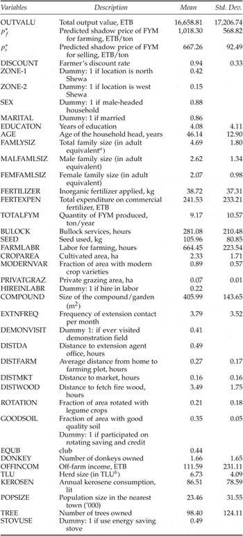
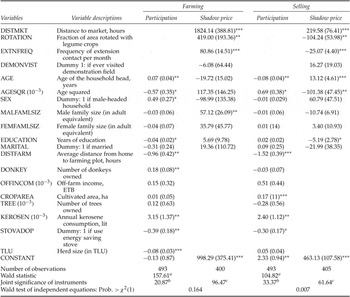
The initial sample contains 500 randomly selected farm households. However, after removing inconsistent and non-systematically missing information, data from 493 farmers remain for use in our empirical estimation. A two-stage cluster random sampling technique was employed for selecting districts and respondents from each area. The sample households were randomly selected from village rosters that exhaustively record all members of the villages. The data set features detailed information regarding household and farm characteristics, such as annual earnings from selling livestock and livestock products, including selling FYM. The selling price of FYM is defined as the quotient of annual earnings from FYM and the total quantity of sales. The FYM price is determined in local markets and, due to the high transaction costs associated with the bulkiness of the product, we exhibit inter-village price variations. Table 1 contains the descriptions and descriptive statistics of the variables used in the estimations.
Definitions, means and standard deviations of variables used in the regressions

aAdapted from the Amsterdam scale (see Deaton and Muellbauer, Reference Deaton and Muellbauer1980).
bHerd size measured in terms of Tropical Livestock Unit where 1 TLU (which equals 250 kg body mass) =1 cattle = 6.67 sheep/goat =1 horse =1.15 mule =1.54 donkey =0.87 mule =200 poultry.
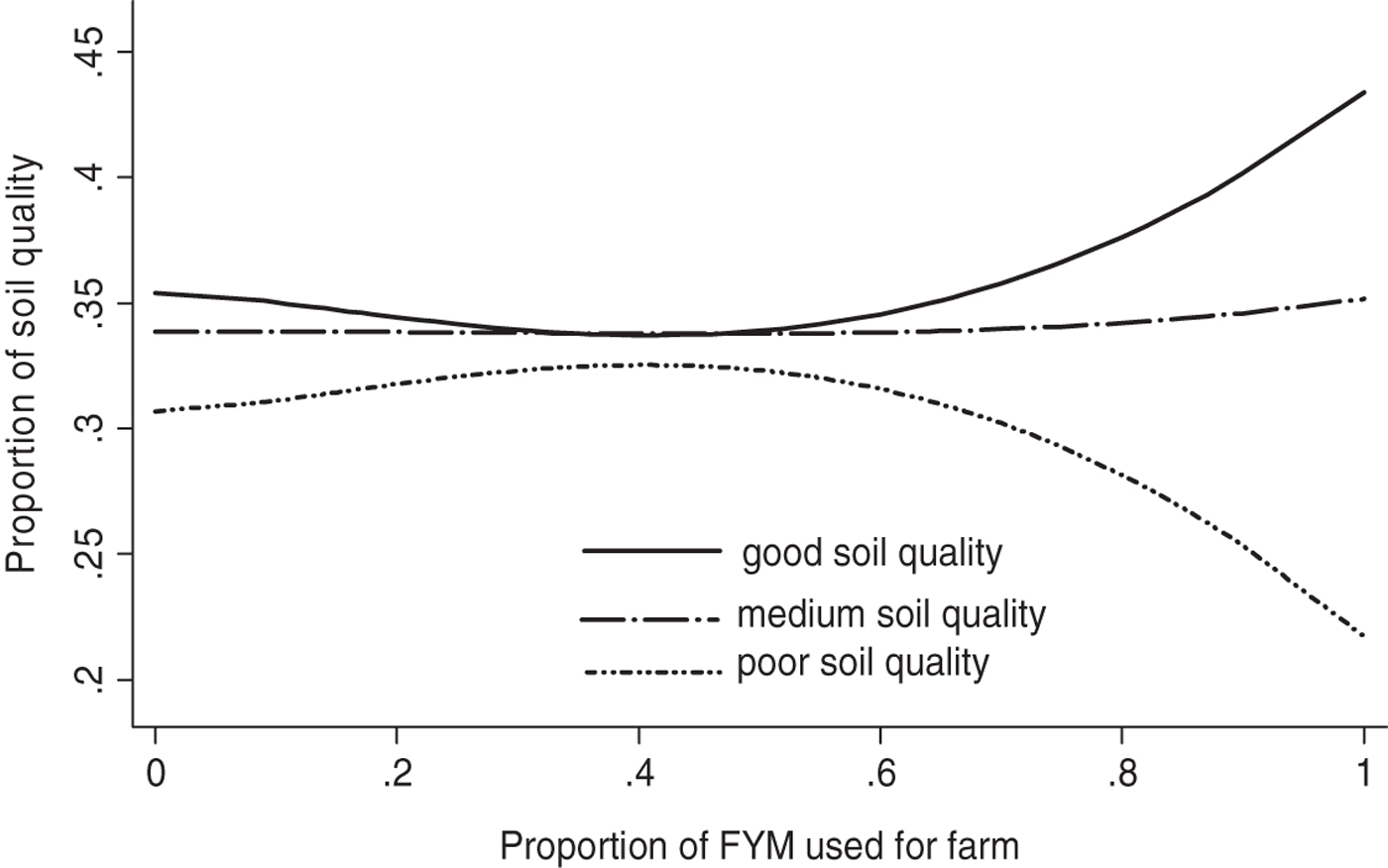
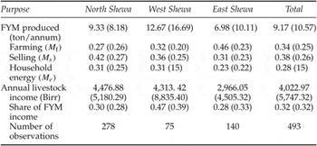
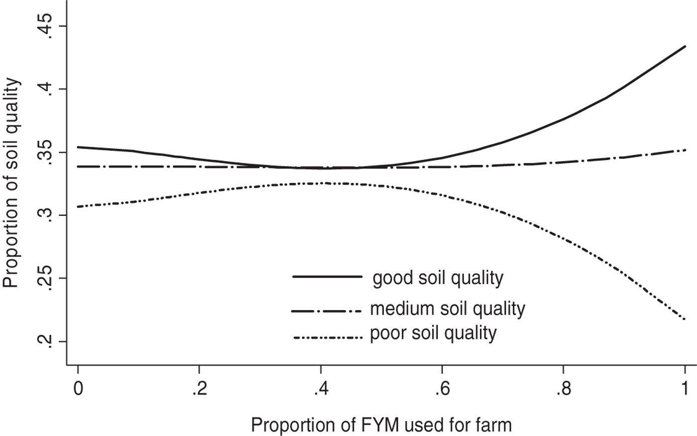
Table 2 presents the farm household's total annual production of FYMFootnote 5 and its use for different activities. FYM selling in the study sites is also an important source of household income, covering 28–47 per cent of total livestock income. The empirical findings concerning the demand for FYM for farming may be more clearly understood if they are prefaced by the respondent's classification of soil quality – an indicator of soil fertility depletion due to lack of organic fertilizer. The survey participants were asked to evaluate the soil quality of their farms according to the local assessment criteria. Accordingly, on average 35 per cent, 31 per cent and 34 per cent of the respondents' farms, respectively, were classified as having good, medium and poor soil quality. Despite the positive correlation between good soil quality and FYM used for farming (figure 1), having farming plots with medium and poor soil quality might be an indication that such plots need more FYM to improve the soil.
Correlation between soil quality and FYM used for farming
Average shares of FYM by purposes, contribution of FYM to annual livestock income

Note: Numbers in parentheses are standard deviation.
In this study, to elicit the farmer's discount rate, a simple choice task was used. This is the most common method for eliciting time preferences (Pender, Reference Pender1996; Holden et al., Reference Holden, Shiferaw and Wik1998; Frederick et al., Reference Frederick, Loewenstein and O'Donoghue2002; Bezabih, Reference Bezabih2009; Yesuf and Bluffstone, Reference Yesuf and Bluffstone2009). All sample respondents in the household survey were confronted with a hypothetical experiment designed to elicit their willingness to delay current consumption. Here, subjects were asked to choose between a smaller, more immediate reward and a larger, more delayed reward. This is the choice between the hypothetical future value payable after one year (almost one growing season) equivalent to a fixed present value. As discussed by Frederick et al. (Reference Frederick, Loewenstein and O'Donoghue2002), to precisely estimate the discount rate and to avoid a single choice between two inter-temporal options that only reveal an upper or lower boundary of the discount rate, this experiment presented a progression of choices that vary by the amount of delay rewards. Hence, a series of six binary choices between the specified amounts of wheat grain to be received now (50 kg) or the alternative amount of wheat grain to be given a year later (65, 80, 105, 130, 160 and 195 kg)Footnote 6 were presented in the order mentioned to show which option the farmer preferred within each choice pair (see appendix B for a description of the experiment).
A few words of caution about the hypothetical approach are in order. One limitation of the hypothetical choice experiment is the uncertainty regarding whether people are motivated to do as they would do if outcomes were real (Frederick et al., Reference Frederick, Loewenstein and O'Donoghue2002). Becker and Mulligan (Reference Becker and Mulligan1997) and the references therein also state that, in imagining future wants, the rate-of-discount factor grows larger as the future becomes more remote. However, one can also note that the formulation of large-stakes rewards in a one-year timeframe, as in this experiment, might agree with the actual yearly agricultural production cycle, but in terms of cost it is also difficult to conduct with real rewards. Like all experimental elicitation procedures, the results from such types of choice tasks can also be affected by procedural nuances such as the anchoring effect that occurs when respondents are asked to make multiple choices between immediate and delayed rewards; the first choice they face often influences subsequent choices (Frederick et al., Reference Frederick, Loewenstein and O'Donoghue2002).
5. Empirical results
5.1. Estimation of shadow values
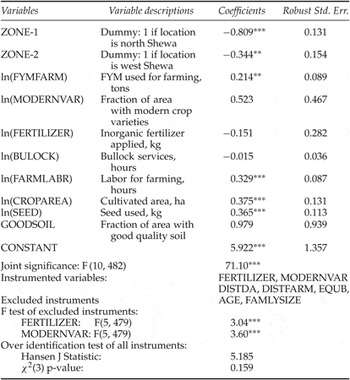
The first step in the empirical analysis is estimation of the agricultural technology to obtain the marginal revenue product of FYM. Table 3 reports the instrumental variable (2SLS) estimates of the agricultural production function. This estimation is based on farm inputs and the total value of outputs recorded during the main growing season of the 2006 cropping period.Footnote 7 The results show that agricultural output significantly increases with the application of FYM. Output is also positively correlated with labor input, seed and cultivated land area. A concern in the estimation of agricultural production function is that agricultural outputs are in part determined by the agricultural activities chosen by the farm households, a worry for the possibility of simultaneity bias. Because of the expectation of reverse causality that inorganic fertilizer and modern seed varieties are determinants of agricultural output and are hence assumed to be potentially endogenous, the model is estimated using an instrumental variable. The choice of instruments for the endogenous regressors in this case is hypothesized to satisfy the relevance and validity conditions in which the instruments are engaged. The application of inorganic fertilizer and modern seed varieties are partly related to the farmer's access to information and household and farm characteristics.
Instrumental variable (2SLS) estimation of agricultural production function (dependent variable: ln (OUTVALU))

Notes: **, *** refer to significance level at 5% and 1%, respectively.
The correlation of the included endogenous regressors with the instruments can be assessed by an examination of the explanatory power of the excluded instruments in the first-stage regressions. The F-statistics in the first-stage regressions for both endogenous variables are jointly significant at the 1 per cent level, which satisfies one condition that ensures instrument validity. However, for models with more than one endogenous variable, as specified here, these indicators may not be sufficiently informative. The Hanson J-test of over-identifying restriction is found not to be significant and therefore confirms the validity of our instruments to satisfy the orthogonality condition required for their employment.
The marginal product of FYM estimated from the production function is observed only for FYM farming participant farmers. Not observing marginal productivity is likely to be indicative of non-participation in FYM farming. Hence, marginal products are imputed for each observation by estimating participation and marginal product equations jointly, matching with the household, farm and village characteristics. This is used to estimate the parameters and thus predict the shadow value of FYM in farming for each observation. Table 4 presents the maximum likelihood result of the determinants of participation in FYM farming and the return from it. Sample selection bias here may be due to self-selection by the farm households who found FYM farming to be more advantageous (due to pre-existing conditions or attributes) than non-FYM farming. Similarly, the shadow return of FYM selling is predicted for each observation by estimating market participation and selling price jointly.
Maximum likelihood estimate for participation and shadow values of FYM

Notes: *, **, *** refer to significance level at 10%, 5% and 1%, respectively; parenthetical terms are robust standard errors.
aWald test for joint significance of the explanatory variables distributed as a chi-square with critical values of 27.69 for 13 degrees of freedom at 0.01 probability.
bJoint significance of the instruments (DISTFARM, DONKEY, OFFINCOM, CROPAREA, TREE, KEROSEN, STOVADOP and TLU) distributed as a chi-square with critical values of 20.09 for 8 degrees of freedom at 0.01 probability.
cJoint significance of the instruments (ZONE-1, ZONE-2, EXTNFREQ and DEMONVIST) distributed as a chi-square with critical values of 13.28 for 4 degrees of freedom at 0.01 probability.
Location controls are included but not shown here.
There are different factors determining the selection process. As expected, with the additional eight variables that are included in the participation equation (for both FYM farming and selling), the outcome equations are jointly significantly different from zero (χ2(8) = 33.37 with a p-value of 0.001 for FYM selling; and χ2(8) = 20.87 with a p-value of 0.008 for FYM farming). The results suggest the identifying variables are successful at enabling identification. Hence, these variables are important for explaining participation of FYM farming and selling equations. The fitted shadow value of FYM in farming and selling from the above procedure is derived and kept for use in the FYM allocation model. Wald tests for the joint significance of the instruments used in each shadow value equation are presented in table 4.Footnote 8 At 0.01 probability, the instruments are jointly significant. This result confirms that our instruments are informative for the identification of FYM allocation equations. A note of caution is that, while the instruments are globally statistically significant, individually some instruments are weak.
5.2. Testing equality of prices
In theory, an individual allocates scarce resources among various alternatives until the point at which the marginal returns across alternatives are equal. By doing so, farmers could choose the most profitable alternative options. For instance, if the productivity of FYM in farming is higher than the return of FYM from selling, it pays for farmers to shift FYM resources into farming and away from selling in the market. It has been observed that the average selling price of FYM (ETB 667/ton) is significantly lower (t-value = 13.21) than the average marginal revenue product of FYM (ETB 1018/ton), but it is significantly higher (t-value = 7.36) than the discounted marginal revenue product (ETB 544.74).Footnote 9
In order to formally test whether the FYM allocations are efficient, the equality between the estimated marginal returns of FYM and the observed FYM price from the markets is tested. This test could shed some light on the presence of farm household preferences that are relevant for determining the allocations. Following the approach of Jacoby (Reference Jacoby1993) and Skoufias (Reference Skoufias1994), who relate market wage with marginal productivity of labor in their agricultural labor supply analyses, we regress the discounted marginal product of FYM on the selling price as follows:

where p f* is the discounted marginal revenue product of FYM in farming; p s* is the FYM price by selling on the market; and v is the random disturbance.
The regression result from (6) is shown as:Footnote 10

The null hypothesis of efficient FYM allocations is contained in the conditions that (γ, φ) = (0, 1). The value of F-statistics for H 0 : γ = 0 and φ = 1 is 139.26; and the 5 per cent critical value of F(2, 491) is 3.01. The value of the joint F-statistics rejects the hypothesis at standard significance levels. As explained by Skoufias (Reference Skoufias1994), these test results provide evidence contrary to the efficient operation of the market, and thus indirectly support the concern about non-separability between the production and consumption decisions of farm households. It is possible that there are other explanations for the rejection of the equality of the two values (p f* and p s*). Often the treatment of households' resource allocation behavior, which creates a wedge between the marginal revenue product and observed market price, could be related to household characteristics and constraints on factor availability and market imperfections (Jacoby, Reference Jacoby1993). Another explanation from Jacoby (Reference Jacoby1993) for this rejection is based on the grounds that the estimated marginal products may in fact be systematically biased so that the instrumental variable method does not lead to consistent estimates. The next section explores the relationship between shadow prices, farmers' impatience and FYM allocations.
5.3. Shadow prices on farmyard manure allocation
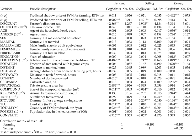
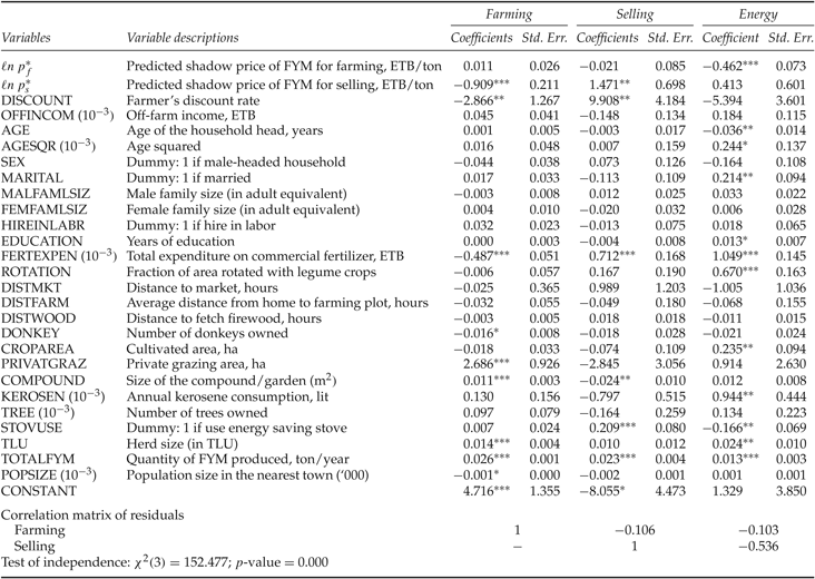
The estimated shadow values predicted in the first stage of the analysis together with farmers' degree of impatience and other socioeconomic information were matched with the individual farm household FYM allocation data. The estimation results are presented in table 5. The estimated model performs well. The calculated χ2-statistic of 4702.75 is statistically significant at the 1 per cent significance level, providing evidence for the hypothesis of joint significance of the explanatory variables across all equations. As expected, the test of independence confirmed the rejection of the null hypothesis, which states that the covariance of the error terms across equations is not correlated. The test supports the estimation with SUR [χ2(3) = 152.477 with the associated p-value of 0.000]. The estimates of FYM allocation functions with a full set of regressors provide empirical evidence on the effects of the shadow value of FYM-affecting allocations across different purposes. The coefficients for shadow prices ℓn p s* and ℓn p f* provide estimates of the uncompensated own-price elasticity for FYM farming and selling, respectively.
Maximum likelihood estimates for FYM allocation
Note: *, **, *** refer to significance level at 10%, 5% and 1%, respectively.
The results also provide the uncompensated cross-price elasticity for FYM farming, burning and selling. The estimated results are in agreement with the expectations. The point estimate of the return of FYM from selling (ℓn p s*) and farming (ℓn p f*) in the FYM farming equation is negative but individually statistically different from zero at the 1 per cent significance level for selling price only. The negative sign of FYM selling price in the farming equation indicates the expected cross-price effect; as the selling price of FYM increases, the farmer responds by allocating less to farming. The estimate for uncompensated elasticity is that a 1 per cent increment of the selling price of FYM leads to an approximately 1 per cent decline of FYM for farming. This jeopardizes a smallholder's soil fertility maintenance with adverse implications on sustainable management of one of the most important natural resources.
The point estimates for the FYM selling price in the FYM selling equation are positive and statistically different from zero at the 5 per cent significance level. As expected, the findings reveal that farmers rationally respond to the change in price of FYM in the allocation of FYM for selling. As for allocating FYM for selling, it basically depends on the extent of the change in FYM for farming and the change in a household's consumption of energy from FYM burning. The increase in the selling price of FYM increases the price in terms of burning at home, thereby making burning FYM more expensive. This substitution effect, then, tends to cut the amount of FYM allocated for household energy. The uncompensated cross-price elasticity is positive but not significant.
5.4. Farmer's impatience on allocation of farmyard manure
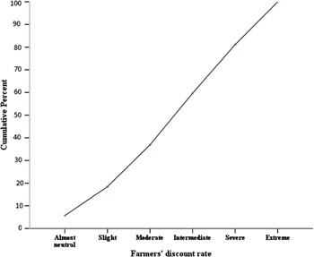
Typically, individuals show a systematic preference for receiving a reward immediately rather than at some later moment in time. When a respondent shifts preference from the early amounts to the amount for a later reward, the implicit one-year rate of time preference was calculated as follows: δ = ℓn(f/p), where the respondent is indifferent between an amount of p at the current time and a reward of f received one year in the future (appendix B). The mean discount rate in this experiment is about 94 per cent. Pender (Reference Pender1996), however, reported a discount rate of 30–60 per cent for Indian villages, whereas Holden et al. (Reference Holden, Shiferaw and Wik1998) found a mean discount rate of 93 per cent for Indonesia, 104 per cent for Zambia and 53 per cent for one village in Ethiopia. Similar to Holden et al. (Reference Holden, Shiferaw and Wik1998) and Pender (Reference Pender1996), who found an upward bias from their experiment that asked farmers to adjust a present value equivalent to a fixed future value, about 64 per cent of farmers in this study were found to have a high discount rate (95–135 per cent) in an experiment that asks the future value equivalent for a fixed present value (figure 2).
Farmers' discount rate responses for future value equivalents

From the foregoing discussions, the marginal return of FYM in farming is higher than the price of FYM from selling on the market, although the former presents a delayed outcome while the latter presents immediate benefits. The parameter estimates for the farmer's discount rate are in agreement with the expectation in the FYM allocation equations. The point estimate of farmers' degree of impatience in the FYM-selling equation is statistically different from zero at the 95 per cent confidence level. The positive sign indicates that farmers with a high degree of impatience increase allocation of FYM for selling. The theory that people with a positive time preference show a preference for receiving a commodity immediately is consistent with behaviors observed in the FYM-selling equation. Here, farmers usually receive the return immediately, so that, of the available options, it is the option of choice for impatient farm households.
In contrast, the farmer's degree of impatience negatively affects the allocation of FYM for farming and burning, but the effect is statistically significant in the former case only. The outcome of allocating FYM for farming is quite remote due to the seasonality in agriculture, forcing the impatient farmers to switch away from FYM farming. Smallholders operating under imperfect credit market settings may not invest their FYM today to increase the future agricultural productivity of their farms when the alternative of selling FYM is possible to meet immediate subsistence needs. The absence of credit for investing in on-farm improvements or consumption credit to meet immediate needs induces underinvestment and sacrifices the quality of the soil, resulting in lower future productivity and persistent poverty (Marenya and Barrett, Reference Marenya and Barrett2007).
This result is in accord with the few other studies that combine time preference experiments with field observations for better understanding of field behavior. An empirical study of Ethiopia (Shiferaw and Holden, Reference Shiferaw and Holden1998) found a negative correlation between an individual's rate of time preference and adoption of soil conservation technologies. In Brazil, impatient fishermen in a time preference experiment exploited the fishing grounds more (Fehr and Leibbrandt, Reference Fehr and Leibbrandt2008), whereas people in Sri Lanka with a higher rate of time preference extracted more non-timber forest products, causing depletion of forest resources (Gunatilake et al., Reference Gunatilake, Wickramasinghe and Abeygunawardena2007). Therefore, a high rate of time preference is an important constraint for investments in soil conservation and could be viewed as a cause of the continuous depletion of soil resources. In this context, the allocation of FYM in farming plots can be considered a present investment to improve soil fertility, thereby improving future agricultural productivity and returns. The policy implication of this is that fixing the broken credit market is important for investing FYM as soil fertility.
Table 5 also provides several factors that are obvious determinants of the allocation of FYM for the different activities. We find statistical evidence for the change in allocations of FYM for household energy over the life cycle. Our findings show a U-shaped relationship between age and consumption of FYM for household energy. Households spend less FYM for energy until they reach a certain age (around age 70), after which consumption is increased. Herd size (TLU) is a resource variable that provides a good indication of a household's wealth status. The result shows that wealthier households spent more FYM for farming and burning in the households. TLU could also approximate the household's capacity to produce more FYM. The result shows that, as the capacity to produce FYM increases, the amount of FYM spent for farming and burning in the household increases as well. This result corroborates the effect of the quantity of FYM produced at the household level. As production of FYM increases, the amount of FYM allocated for each purpose is increased significantly. The size of the effect is higher for selling and farming, however.
We observe a negative and statistically significant relationship between expenditure on inorganic fertilizer and FYM for farming, suggesting substitutability between FYM and inorganic fertilizer. Although the complementarity is likely due to the beneficial interactive effects of FYM on fertilizer efficiency (Marenya and Barrett, Reference Marenya and Barrett2007), the substitutability is important for poor smallholders, as they use lower quantities of commercial fertilizers largely due to high price as well as liquidity constraints. The positive and statistically significant coefficients of fertilizer expenditure on FYM selling and burning in the household would seem to show an increase in quantity of FYM for selling and burning in the household when inorganic fertilizer substitutes for FYM for farming.
We find a positive and statistically significant coefficient of the ‘KEROSEN’ variable in the FYM-burning equation.Footnote 11 A possible explanation is the complementarity between consumption of kerosene and FYM used for household sources of energy, though the size of the effect is very small (the elasticity is about 0.08). In rural Ethiopia it is not uncommon to use kerosene as a source of lighting. The coefficient of use of improved stoves in the FYM-burning equation is negative and statistically significant, however. This coefficient is a measure of the technical substitution (Amacher et al., Reference Amacher, Hyde and Joshee1993) of stoves for FYM, suggesting that improved stoves reduce household FYM consumption by about 15 per cent. This result is consistent with Mekonnen and Köhlin (Reference Mekonnen and Köhlin2008). The same study also indicated that encouraging households to use more efficient cooking stoves is a possible solution to the problem of the limited use of dung as manure. We also observe a positive and statistically significant correlation between use of stoves and FYM selling.
6. Conclusions
The causes of soil fertility depletion extend beyond the farm, receiving effects from market fundamentals and farmer preferences. The main contributions of this study are the analyses of the effects of various returns of FYM and farmers' impatience with the trade-offs of using FYM as inputs to agriculture or burning FYM within or outside of the household. The empirical analysis is based on a system of equations for the farmers' allocation of FYM for different purposes. The farm household survey data comes from the central highlands of Ethiopia, where a mixed crop-livestock farming system is practiced. The data support the predictions and show that the farmer's time preference and the returns to FYM are important predictors of the allocation of this multi-purpose resource in the real world. Farmers with a high degree of impatience decrease the allocation of FYM to the farm. The higher the selling price of FYM, the higher the incentive for farm households to sell FYM for burning outside the farm households.
In smallholder agriculture, where agricultural productivity remains low, the returns from selling FYM will increase as the demand for biomass fuel rises and supply declines. In Ethiopia, where fuel prices have been rising and electricity infrastructure is poor, there is growing interest in using FYM for energy production. In order to encourage adoption of FYM farming as sustainable land management practice, the results suggest that incentive policies may be developed in conjunction with the fuel-pricing system, including substitution and energy conversion technology such as promotion and dissemination of improved stoves not only to the rural areas but also the surrounding towns.
The high discount rate of the poor due to serious imperfections in the credit markets has received previous attention (Pender, Reference Pender1996; Becker and Mulligan, Reference Becker and Mulligan1997; Holden et al., Reference Holden, Shiferaw and Wik1998; Bezabih, Reference Bezabih2009; Yesuf and Bluffstone, Reference Yesuf and Bluffstone2009; Tanaka et al., Reference Tanaka, Camerer and Quang2010). The high discount rates observed in this study, on the other hand, indicate the disregard of most farm households for the use of FYM farming with effects on sustainable management of the soil resources. This implies that the poverty reduction scheme and ensuring the functioning of rural credit markets are also important policy directions associated with sustainable land management practices.
Appendix A: FYM-allocation model
The model presented below captures the case of a farm household involved in a mixed farming system, where FYM (Q m) is one of the most important byproducts of the system, assumed to be a function of the vector of farm inputs and structural characteristics of the farm household. Utility is derived from consumption of agricultural and purchased goods (C), energy (E), and leisure (L l). The demand for FYM burning at the farm household level is a derived demand from the demand for energy (E), where energy is sourced from FYM (M e) and other sources such as kerosene and other biomass (O e). Agricultural production (Q a) takes place on individual plots using organic (FYM) and inorganic fertilizer. We assume inorganic fertilizer is the purchased variable input, while FYM is obtained from livestock production within the farm households.
Given a total amount of FYM at the farmer's disposal, the farmer's decision consists of allocating Q m between farming (M f), burning in the household (M e), and selling on the market as an additional source of income (M s) for burning outside the household. The implication is that farm households in the area are semi-commercial; even if markets for FYM exist, most retain some FYM for home consumption and farm production. Examination of the data for this study has also revealed that all farm households obtained FYM for burning (M e) and farming (M f) from their own production system without making any purchase. The net marketed amount of FYM is therefore non-negative: Q m − M e − M f ≥ 0. Households also choose the amount of labor for on-farm (L f) and off-farm (L o) activities. The household budget constraint binds the value of consumption of agricultural goods and purchased goods (C) by a household's total income (Y) that originates from agricultural income (π), off-farm work (L o) at wage rate (w) and FYM sales (M s) at a price (p s). Agricultural production is specified as a function of M f, L f and other variable inputs (X), such as inorganic fertilizer, seeds, pesticide, etc. Agricultural income is the farm-restricted profit where the value of the cost of production is subtracted from the total amount of crop produced (p aQ a).
For each year, the agricultural season is divided into the wet or planting season and the dry or harvesting season. The nature of the agricultural production is such that for FYM applied to the field during the planting season, agricultural output is expected at the harvesting period. In Ethiopia, where agricultural production is mainly rain fed, this is nearly a year-round process. Investing FYM on the farm means postponing the current consumption originated from burning FYM in the household or income earned from selling FYM on the market. This loss, interpreted as the benefit obtained from selling or burning FYM now, is assumed to be compared and offset by the discounted returns of FYM in farming at a later time. When imperfect credit markets prevent perfect consumption smoothing, depending on the individual implicit discount rate, farmers often opt to sell or burn FYM, which limits their ability to use FYM for farming. Hence, with the subjective discount rate parameter (δ), the relationship between time preference and allocation behavior is more pronounced. A farmer's discount rate is expected to affect household resource allocation following the standard intuition: a higher δ should result in higher resources toward current consumption. Formally, given these specifications, farmers are assumed to choose M f, M e, M s, L l, L f, L o, and X so as to:

subject to farmers' resource and productivity restrictions:


where Z c and Z q are vectors of household and farm characteristics influencing preferences and farm production, respectively.
Substituting the constraints into the utility function above and assuming the farm household's choice at the start of the dry season, we can specify the Lagrangean as:

where λ is the Lagrangean multiplier associated with income constraints and ηf, ηe and ηs are Lagrangean multipliers associated with inequality constraints on FYM farming, burning and selling, respectively.
Maximization of the Lagrangean with respect to M s, M f and M e provides the following first-order conditions:
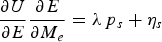

The above first-order conditions indicate that, at the optimum, farm households allocate FYM across alternative options so as to equate the marginal value of household energy from FYM with that of FYM spent on selling (A.9) or farming (A.10) – that is, the discounted future marginal revenue product from agricultural production or net returns from marketing. In other words, the discounted gains from the extra increment of future agricultural production due to improved soil fertility and the net returns from FYM selling are equalized to the household-specific opportunity cost of FYM for burning. The complementary slackness condition for constrained maximum in equation (A.9) and (A.10) may infer the shadow price of FYM for selling and farming, respectively. When households optimally allocate FYM in the market and in farming, the shadow price of FYM selling (p s* = p s + ηs/λ) and FYM farming (p f* = (1/δ) p a (∂ Q a/∂ M f) + ηf/λ) is equal to the respective observed FYM price (p s* = p s) or the discounted marginal value product of FYM (p f* = (1/δ) p a (∂ Q a/ ∂ M f)). This is because, for an interior solution, the complementary slackness condition requires ηi = 0 given (M i > 0; for i = f, s).
However, again following the complementary slackness condition that requires ηi > 0 for a farmer who exhibits corner solutions (M i = 0; for i = f, s), the shadow prices, p s* and p f*, will be in general greater than the observed selling price and the marginal value product, respectively. The shadow prices of FYM are measured in real terms denoting the unobservable internal prices in the case of non-separability. They may be defined as the market price or returns plus the value that farmers assign to themselves for supplying or not supplying FYM to the market or to the farm. Thus the shadow prices of FYM are endogenously determined by parameters affecting the household's production and consumption decision variables. The first-order conditions above can be combined to derive a set of reduced form of Marshallian demand functions for FYM for farming, for household energy, and the supply of FYM for selling in the market. These are expressed as functions of shadow prices, farmer's time preference, and other individual and farm characteristics:

Appendix B: Structure of the time preference experiment and farmer's discount rate
Instruction
We would like to know your preference for taking wheat grain now compared to taking wheat grain after a year. Please indicate for each of the following number of choices, whether you would prefer to receive the smaller amount of wheat now or the bigger amount of wheat one year from now. For instance, which would you choose: 50 kg wheat now or 65 kg wheat exactly after one year?

aThe implicit one-year discount rate: δ = ℓn(f/p)
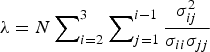 . λ has a χ2 distribution with three degrees of freedom.