1. Introduction

Dynamic-thermodynamic sea-ice models (e.g. Reference HiblerHibler, 1979; Reference Tremblay and MysakTrembly and Mysak, 1997; Reference Zhang and HiblerZhang and Hibler, 1997; Reference Geiger, Hibler and AckleyGeiger and others, 1998) used to simulate sea-ice drift and deformation make use of highly non-linear plastic rheologies. While these rheologies modify the ice drift, their most significant effect is to modify the deformation of pack ice. Recent advances in the acquisition and analysis of satellite-based synthetic aperture radar (SAR) images (Reference Kwok, Dempsey, Shen and ShapiroKwok, 2000) show that spatial patterns of ice deformation in the Arctic basin are dominated by relatively narrow deformation patterns that in many cases open to form leads which in turn control air-sea heat exchanges in pack ice. In addition, local observations of deformation (Reference Hibler, Weeks, Kovacs and AckleyHibler and others, 1974; Reference Heil, Lytle and AllisonHeil and others, 1998) show leads to be opening and closing on a relatively rapid basis with considerable power near the inertial period. Estimates of ice growth due to such high-frequency deformation components (Reference Heil, Lytle and AllisonHeil and others, 1998) have shown that in the Antarctic pack ice higher-frequency components can contribute as much as 50% to the overall ice growth. Hence, simulating such features and their variations may have considerable relevance to air-sea heat exchanges and to developing a better understanding of the processes contributing to overall Arctic ice-pack thinning or thickening.

Examination of these lead patterns using observed imagery of the Arctic basin shows them to have a substantial similarity to fracture patterns observed in failure of laboratory sea ice under biaxial compression (Reference Schulson and HiblerSchulson and Hibler, 1991; Schulson, 2000). These lead patterns are also found to shift in response to the wind forcing which supplies the main variable driving body force for floating pack ice. They have also been found to occur regularly in near-shore regions (Reference Overland, McNutt, Salo, Groves and LiOverland and others, 1998), with geographical boundaries playing a major role in their formation and location. Correlations of mean lead orientation with wind fields (Reference Barry, Miles, Cianflone, Scharfen and SchnellBarry and others, 1989) have also shown that such fractures on average tend to align with the geostrophic wind. However, examination of the evolution of SAR deformation features (Reference Kwok, Dempsey, Shen and ShapiroKwok, 2000) shows considerable persistence of such features even as winds change on weekly time-scales.

The similarity of these features with laboratory-based results (see, e.g., Schulson, 2000) suggests that such oriented patterns are almost certainly ice-mechanics features with substantial fracture-based mechanisms operating in their formation. Recent theoretical anisotropic models of pack ice (Reference Hibler and SchulsonHibler and Schulson, 2000) have been developed which hold the promise of simulating both oriented leads and deformation patterns. The main operative mechanism in these models is the classic concept of failure along oriented features where shear stress becomes maximized or very large. The work of Reference Hibler and SchulsonHibler and Schulson (2000) generalized the classic local frictional "Coulombic" model to finite oriented zones of failure. In the case of a finite zone of failure, both the yield and flow characteristics in the failure zone will affect the preferred orientation of the failure patterns. As part of this anisotropic model, Reference Hibler and SchulsonHibler and Schulson (2000) also proposed a modified Coulombic yield surface that yields intersecting leads with intersection angles of ∼45°.

To proceed from oriented failure to the full formation of leads requires some type of weakening of the ice as deformation occurs. In this paper we focus on the effects of weakening on forming oriented zones of deformation and also examine the degree to which high-resolution isotropic models can simulate such features within the Arctic basin. The concept here is that weak features, once formed, act as major stress concentrators within the ice pack. Since isotropic models are much more easily implemented in large-scale climatic models and can be formulated to insure energetic consistency, they may be more useful in many contexts. To address these issues here, we first extend the basic anisotropic model of Reference Hibler and SchulsonHibler and Schulson (2000) to allow weakening of multiple-oriented leads with varying strengths locally. Using this framework together with more traditional isotropic models, a comparative set of simulations is carried out with fixed wind forcing and with weakening due to divergence. These results are analyzed to examine the character of the concentrated shear zones developed, the character of lineated features in the weakened ice and the dependence of these features on rheology, both anisotropic and isotropic.

2. Localized Failure Model and Characteristic Observations

The basic observational characteristics for which we wish to develop a modeling capability are shown in Figure 1. These observations show concentrated patterns that tend to intersect and are highly localized. A notable feature of these observations is the localization of the deformation into narrow bands so that the strain varies spatially in a relatively discontinuous manner. Another feature is that statistical estimates of the intersecting angles (Reference Cunningham, Kwok, Banfield and SteinCunningham and others, 1994) of the leads tend to be focused around 40°. The precise reasons for this are still largely unexplained, although the theory of Reference Hibler and SchulsonHibler and Schulson (2000) showed that with the appropriate flow rule such angles are consistent with laboratory (Reference Schulson and NickolayevSchulson and Nickolayev, 1995) brittle-failure yield curves.

Fig. 1.

Maximum shear deformation obtained from sar imagery over a 500 × 500 km₂ region in the western beaufort sea. the results are plotted at a 10 km resolution and are based on differential positions of a variety of location points on the ice on julian days 331−334 in 1996 (personal communication from r. kwok, 1999).

A modeling capability relevant to these features based on a finite-width failure model (similar to Fig. 2) has been developed by Reference Hibler and SchulsonHibler and Schulson (1997, Reference Hibler and Schulson2000). However, Reference Hibler and SchulsonHibler and Schulson (2000) only considered idealized fixed-stress-state numerical experiments and did not examine in detail the formation of fractures in basin-wide numerical simulations. Also the effect of weakening on the damage formation was not examined. To extend this model to a fully anisotropic model with weakening, it is necessary to generalize the localized model to include multiple-oriented leads with different strengths, and to provide a weakening mechanism as deformation occurs.

Fig. 2.

Schematic of boundary conditions for two or more leads for constructing anisotropic failure characteristics of a composite comprised of noriented leads in thick ice.

2.1. Anisotropic failure model for multiple-oriented leads

The basic idea in anisotropic models is to consider oriented leads in thick ice (Reference Coon, Echert, Knoke and HrudeyCoon and others, 1992, Reference Coon, Knoke, Echert and Pritchard1998; Reference Hibler and SchulsonHibler and Schulson, 1997, Reference Hibler and Schulson2000). To extend a single-oriented lead to multiple-oriented leads, we consider a variety of oriented leads with different ice thicknesses as in Figure 2. In this case we have continuity of stresses at the boundary faces of all leads, and the total strain must be made up of the aggregate strain of all the leads and the thick ice. Considering an arbitrary coordinate system we have by Green’s theorem for n leads

(1)

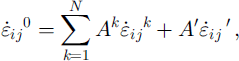
where a superscript zero denotes the whole composite, the superscript k denotes a particular lead, and the primed values refer to the thick ice. In Equation (1), A^k and A’ are the fractional area of the κth lead and the thick ice respectively. To determine the strain rates and stresses in each lead we take and to be the strain rates and stresses of each lead in a coordinate system aligned with the lead with the y axis along the strike of the lead. Denoting these rotated strain rates with italic letter subscripts, the strain rate along the lead is taken to be the same as the component of the composite strain rate in the same co-ordinate system aligned with the lead.

The remaining strain rates in the lead and are determined by insisting on stress continuity across the face common between the lead and the thick ice. Assuming that the stress state of both the thin and thick ice may be expressed in a special form of the Reiner-Rivlin constitutive law,

(2)

The continuity of stresses (along a surface aligned with the lead) leads to two non-linear equations for the ith lead

(3)

(4)

where the bulk and shear viscosities ζ and _η depend on the strain rates in the leads or the thick ice, and the italic letter subscripts refer to a coordinate system aligned with the ith lead. Combining matrix equations (1), (3) and (4), we have 2n + 3 independent equations for solving for the 2n + 3 unknowns, and .

To solve these equations we use an iterative procedure whereby the bulk and shear viscosities ζ and η are determined from the strain rates at a previous iteration. The set of Equations (1), (3) and (4) then becomes a linear set of equations for the unknown strain rates. The solution of these linear equations may be obtained by specifying the strain rate of the thick ice and then using Equations (3) and (4) to solve for the strain rates of each lead for stress compatibility. This procedure is carried out independently of the strain-rate constraint expressed in Equation (1). However, by carrying out this calculation for three independent strain rates of the thick ice, the three strain-rate equations of Equation (1) provide three independent equations to solve for the needed strain rates in the thick ice and hence also in the individual leads. In particular, considering perturbed strain rates in the thick ice of

we wish to solve for λ_n(n = 1, …3) such that the overall strain rate is consistent with Equation (1). By noting that a perturbation leads to aggregate strain rates and (and similarly for the other perturbations), the equations for the λ_n become

These equations may be solved using normal linear algebra procedures. Once this is done, the new strains are used to solve for the updated non-linear viscosities, and the procedure is carried out repeatedly until a solution is obtained.

To carry out these anisotropic solutions, we need to specify a yield curve for the thin and thick ice, which for these calculations is assumed to be elliptical as shown in Figure 3a. Shown in Figure 3b is the isotropic Coulombic yield curve used by Reference Hibler and SchulsonHibler and Schulson (2000) to describe the thin ice for one single lead. For the anisotropic study here, we will make use of six oriented leads of differing strengths located at equal 30° intervals which will be allowed to evolve in time. Some of the characteristics of a yield surface resulting from such a collection of leads are shown in Figure 4, where we show failure stresses for six equal-strength leads with one of the leads aligned with the principal axis of the strain rates. While not shown, in the case of, say, one weak lead, the failure stresses become highly orientation-dependent, with stresses applied parallel to the lead becoming very large. However, even in the equal-strength case the yield surface has smooth faces corresponding to failure along only one lead. At the nodes two or more leads are required to fail in order to provide an arbitrary strain rate.

Fig. 3.

Elliptical (a) and "modified" coulombic (b) yield curves. the modified coulombic yield curve has a non-normal flow rule and, for a sample with constant com_pressional boundary stresses σ_× and σ_y, can be shown to yield lead orientations with intersection angles of 40−60° for σ_x/σ_y between 0 and ∼0.2 (see Reference Hibler and Schulsonhibler and schulson, 2000).

Fig. 4.

Yield curve resulting from six equal-strength leads embedded in thick ice with 30° intersection angles, and with the principal stress axes aligned with one of the leads. for other orientations of the principal stresses, the stress and strain-rate principal axes will not be aligned.

For comparative isotropic investigations, simulations with both the Coulombic and elliptical yield curves of Figure 3 will be utilized. While these isotropic simulations are much simpler, the solution procedure in both cases requires producing a given stress in response to a specified strain rate.

2.2. Evolution equations for weakening

To allow weakening to occur, we imagine that in a Lagrangian grid following the ice, weakening can occur in time according to the rate of opening of an individual flaw or lead according to

(5)

where Pi* is the strength of the lead at angle θ_i, is the strain rate perpendicular to the lead, and A is dimensionless. Precisely how to weaken the lead is somewhat arbitrary, but the main physical notion is that formation of open surfaces should occur rather rapidly. As a consequence, in the simulations carried out in this investigation we take A = 400 for all simulations. Also, since we will examine relatively short time evolutions of a few hours, we expect advection effects on these time-scales to be rather small. Consequently we take the substantial derivative equal to the simple time derivative for this study. We also take the area of all leads to be 0.004 and do not allow this to evolve in time. Since single-lead simulations (Reference Hibler and SchulsonHibler and Schulson, 2000) have shown the lead area to hardly modify failure stresses, this constraint is not considered critical.

Since in the anisotropic model the strain rate is concentrated in a single lead at a much higher rate, the evolution for the isotropic case is taken to be

(6)

Here A has been divided by 0.004, which is approximately the scaling factor between the aggregate strain rate and the much greater lead deformation rate.

2.3. Equations of motion and idealized simulations

To solve for deformation and stress fields over a region or for an idealized sample we need to utilize an equation of motion together with either the anisotropic theory described above or an isotropic rheology. In both cases the strain rates for a given gridcell supply stresses to integrate the equations of motion forward in time. For the equations of motion we consider a linearized water drag system with constant turning angles in the atmosphere and the ocean of the form

(7)

where V is the ice velocity, V • • / β = (V× cos / β + Vy,sin β)x - (vy cos β- _vxsin β)y and |τs|= ρ_aC_a|G| where G is the geostrophic wind. A turning angle equal to β is used for the direction of τ_s relative to G. For numerical values we have used _ρwc_w= 0.046 kg m−2 s−1 , _pih = 0.8 × 103 kg _m −2, f = 1.2 × 10−1 s−1, ρaCa = 0.024 kg m−2 s−1 and β= 30°. These values represent relatively small values of water drag but are useful for examining the ability to simulate oriented features by allowing the momentum balance to be more affected by the ice interaction forces. Since the momentum advection term is small (Reference HiblerHibler, 1979), DV/Dt is set equal to the simple time derivative ∂v/∂t.

For boundary value solutions, these equations were explicitly integrated forward in time with 0.05 s time-steps at a resolution of 55 km. For the anisotropic model the initial strengths of the thin ice in all six oriented leads and thick ice (see Fig. 2) were taken to be Pi* = 104 N m−1 and p₀* = 10⁶ N m⁻¹, respectively. As the simulation proceeds, the thin ice automatically weakens or strengthens. In the case of strengthening, the thin-ice strength Pi* is never allowed to become stronger than 25 × 104N m⁻¹ or weaker than 2.5 N m⁻¹. The thick ice does not change its strength, and the areas of the oriented leads are kept fixed at 0.004 times the total area. In the case of the isotropic models, the ice strengths and bounds are the same as used above for thin ice. However, as described above, the weakening employs a larger factor times the divergence rate.

To allow the isotropic model to be compared to the anisotropic case, the same explicit time-stepping procedure is used in all cases. Also, because of the complexity of the anisotropic model, simple four-point differencing of the stress field in a staggered grid is used to calculate the gradient of the stress tensor as the integration proceeds. This procedure produces a less smooth numerical solution than the numerical procedure of Reference HiblerHibler (1979) which has been used in most subsequent investigations of the viscous-plastic sea-ice dynamics model. These equations of motion may also be used to carry out idealized simulations by considering only the acceleration term (lefthand side of Equation (7)) and the stress-gradient term and applying forces to the boundaries of an idealized sample.

An example of a fully anisotropic simulation for an idealized sample is shown in Figure 5. Idealized isotropic simulations (see, e.g., Reference Hibler and SchulsonHibler and Schulson, 2000) carried out with a single flaw show that as the stresses increase, a fracture starts to form and then will eventually propagate through the system. In principle, this fracture should be in the form of alternating leads. Figure 5 shows how this alternating effect naturally develops from the six-lead fully anisotropic model when fixed stresses are applied to the boundaries. In this simulation we started with three specified isotropic weaknesses in an anisotropic system initially composed of six equal-strength leads in every cell. The results show that, as failure occurs, usually only one lead is picked out by the failure process. Consequently, the simulated failure pattern in Figure 6 has smaller flaws clustering along the damage strike. These damage results are at least qualitatively similar to laboratory observations (Reference Schulson, Iliescu and RenshawSchulson and others, 1999).

Fig. 5.

Fracture propagation with weakening with three initial isotropic weaknesses (as shown) for a fully anisotropic model. except for the three center weakened cells, each gridcell contains six oriented weak leads with 30° intersection angles. the lead strengths are initially equal (pi* = 10₄ n m₁). for adequate constant boundary stresses with a confinement ratio of ∼0.1, damage propagates and typically one oriented lead in each grid-cell fails and weakens. the failing oriented leads are shown after the damage has just propagated to the boundaries.

Fig. 6.

(a) Numerical grid with 55 km resolution used for basin-wide simulations. at the "outflow"gridcells denoted by asterisks the ice strength is set equal to zero. other boundaries are closed, (b) velocity field resulting after 1 h, with anisotropic coulombic yield curve including weakening. geostrophic wind contours at ^3 mb contour intervals are overlaid on the velocity solution with a scale of ∼0.5 ms−1 for a vector one gridcell long.

3. Simulations of Basin Oriented Damage Patterns with Anisotropic and Isotropic Models

To examine the ability of isotropic and anisotropic models to simulate oriented damage strikes, we carried out a series of numerical experiments for the Arctic basin using atmospheric forcing during November 1996 when significant lead and deformation activity were observed in the Arctic. An Arctic basin computational grid (Fig. 6a) with 55 km resolution and "open" outflow boundary conditions at the Fram and Bering Straits was used. For this comparison we have carried out two basic sequences of sensitivity studies: first, with a fully anisotropic model with the thickness evolution allowed to evolve; and secondly, similar simulations with two isotropic models (see Fig. 3) employing an elliptical yield curve and the Mohr-Coulomb-like yield curve of Reference Hibler and SchulsonHibler and Schulson (2000). In both these models the velocity field was initialized by carrying out a fixed plastic strength solution with no weakening for about 2.5 × 10³ s. After this the thickness characteristics were allowed to evolve as described above, and the results analyzed to determine equilibrium strength variations.

The ice-velocity field from the isotropic Coulombic simulation, 1 h after weakening was allowed to commence, is shown together with the atmospheric pressure field in Figure 6b, showing an ice velocity which is largely aligned with the geostrophic wind. Due to the low linear water drag, the velocities are relatively large. However, not so apparent from the velocity field is the presence of significant zones of oriented deformation. These maximum shear features are shown in Figure 7 which contours the maximum shear strain rate invariant for the anisotropic model (Fig. 7a) and for the isotropic "Coulombic" yield curve (Fig. 7b). The isotropic elliptical case (Fig. 7c) is generally similar to both these cases, although somewhat smoother with fewer intersecting features.

Fig. 7.

Maximum shear patterns resulting after lh including weakening for different theologies, (a) results for a fully anisotropic model with anisotropic weakening similar to that used in figure 5; (b) results for an isotropic model using the modified coulombic rheology of figure 3b; (c) results for an isotropic model employing an elliptical yield curve (fig 3a). a time-step of At = 0.05 s was used.

The basic damage patterns are qualitatively similar in the three cases, which show concentrated shear patterns largely controlled by the wind field driving the ice and the basic configuration of the basin as well as the available openings from the basin. There is a dominant flow out through the Bering Strait, with a demarcation shear pattern running across the basin that marks a regime of ice motion flowing out through the Fram Strait. The anisotropic model exhibits a somewhat greater degree of intersecting fractures and exhibits this damage pattern at lower values of the wind field.

These simulations were carried out for spatially constant strengths initially, but with subsequent very rapid weakening. In practice, under certain conditions after, say, a wind shift, the ice will be somewhat weaker near the Alaskan coast due to a thinner ice cover. This situation would occur, for example, after a wind event pulling the ice away from the coast. When such weaknesses occur near boundaries, the ice can display more leads. Some of the effects of boundary conditions are illustrated in Figure 8 where the maximum shear contours for the Coulombic isotropic rheology are shown for a zero-stress boundary condition across most of the Alaskan and Canadian Northwest Territories boundary. In this case many more leads tend to evolve with a number of new shear features perpendicular to the previous "closed"-boundary pattern of Figure 7b. Examination of the ice strength shows that there is also less strengthening in the ice pack in the Beaufort Sea. These lead features are particularly coherent in the Coulombic model. It is also notable that in the case of the "open"-boundary condition solution in Figure 8 there is a qualitative agreement between the structure of the simulated maximum shear strikes and those observed by Reference Kwok, Dempsey, Shen and ShapiroKwok (2000) over the time period 28 November-4 December 1996.

Fig. 8.

Maximum shear patterns resulting after ih including weakening with a no-stress "open" −boundary condition along the whole lefthand boundary for an isotropic model using the modified coulombic rheology. a time-step of at = 0.05 s was used.

Although not shown, the evolved strength characteristics (which would essentially represent leads in the case of weaknesses) reflect some of the maximum shear patterns. This is especially true for the open-boundary condition case where more divergence is allowed, and most of the maximum shear patterns in Figure 8 represent weak lineated zones in the ice. Other regions, such as the curving demarcation zone in the shear patterns in Figures 7 and 8, are essentially shear zones with little opening.

A qualitative feature of all the results is a tendency (except for the demarcation zone) for oriented high-shear features to form along the isobars. Since stress-free conditions typically have the ice drifting along isobars, velocity discontinuities along the isobars are easier to develop. Neglecting isobar curvature, such discontinuities are consistent with a stress-free boundary condition on faces aligned with the isobars, but not on faces perpendicular to the isobars.

4. On the Temporal Variability of Deformation

The simulations described above reach an equilibrium after about lh in response to the wind. However, observations (e.g. Reference Hibler, Weeks, Kovacs and AckleyHibler and others, 1974) typically show that deformation fluctuates in time on a much more rapid time-scale than the wind forcing. One likely mechanism for this is the rapid variation of the upper-ocean boundary layer (see, e.g., Reference McPheeMcPhee, 1978) which on time-scales less than a few days does not respond with a passive drag as used in Equation (7). Reference Hibler, Lytle, Heil and LytleHibler and others (1998) in a mechanistic study examined how these boundary-layer effects can couple into kinematic waves in the pack ice and create rapid variations in the deformation. However, the simulations by Reference Hibler, Lytle, Heil and LytleHibler and others (1998) were carried out in a one-dimensional idealized model. To examine how such mechanisms can couple into the two-dimensional fracturing mechanics discussed here, the Coulombic simulation was redone with a more general linearized equation of motion. This equation includes a so-called inertial embedding (Reference McPheeMcPhee, 1978), whereby the oceanic boundary-layer transport is tied to the ice motion and in the steady-state limit reduces to normal water drag. When a small amount of damping was added, Reference McPheeMcPhee (1978) found this model predicted observed ice-drift variability in summer very well over several inertial periods.

To implement this procedure, Equation (7) (see Reference Hibler, Lytle, Heil and LytleHibler and others, 1998, for details) is replaced by

(8)

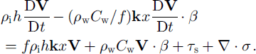
Note in the limit of steady state this equation reduces to Equation (7). To apply this to the Arctic basin the same numerical parameters used by Reference Hibler, Lytle, Heil and LytleHibler and others (1998) are employed, namely, ρ_wc_w = 0.86 kg m⁻² _s−1 / = 14 × 10∼⁴ s−¹, ρih = 10³ kg m⁻². Other constants are the same as noted below Equation (7). Also in this case, because of the increased inertia, a time-step of 0.5 s is allowable and the integration procedure centers the Goriolis terms in time. In a qualitative sense, Equation (8) could be thought of as Equation (7) with rapidly varying external ocean forcing arising from inertial motion in the oceanic boundary layer.

Figure 9 shows some results from this simulation in terms of the evolution of the maximum shear over about lday and the spatial maximum shear pattern at about 22 h. The main result is that the shear pattern oscillates in time, with some shear regions becoming inactive for some period of time. After about 2 days for this fixed wind field, the fluctuating character is reduced and the fracture pattern stabilizes. The main result here is that the coupling between the ice mechanics and ice boundary-layer motions results in a fluctuating deformation field that is still controlled by the fracturing process. While the simple embedded linear model used above is probably somewhat underdamped due to the neglect of oceanic processes that can remove inertial energy this simulation does supply a credible explanation for the fluctuating character of ice deformation which is typically observed in pack ice with precise deformation measurements.

Fig. 9.

Shear-deformation results when "inertial embedding"is included, (a) spatial shear-deformation period after ∼22h and part (b) shows the evolution of the maximum shear rate (multiplied by −2 and smoothed with a 9 point hamming filter) for a transect along the × axis (fry =24) as a function of time.

Discussion

The main focus of the model development and numerical simulations here has been to investigate the ability of nonlinear plastic models currently used in many climate investigations to simulate oriented leads and fracture patterns. The basic theory for such features is contained in the concept of a finite-width failure zone which tends to lead to preferred oriented failures in plastic flow in a manner consistent with continuity-of-stress arguments. These oriented failure strikes can be obtained by inserting weaknesses in a localized region of otherwise constant stress. In basin-wide simulations they can be induced by starting with a constant-strength system, but having irregular boundaries and a complex body forcing on the system via a spatially varying wind field.

Looking in detail at the deformation pattern from a viscous-plastic equilibrium solution, oriented failure patterns naturally occur with constant isotropic strength. The main selection process occurs once the ice starts to weaken. If the ice is allowed to strengthen either anisotropically or in an isotropic manner without changing the wind field, there is a consolidation of the failure to fewer overall faults. The effects of anisotropic weakening with fixed wind fields appear to create a somewhat larger number of faults because failure can occur along oriented weaknesses that approximately align with the fault strike. However, qualitatively the differences from the isotropic case utilizing a "modified" Coulombic rheology are not large.

Since these oriented failure patterns are relatively ubiquitous in an equilibrium plastic solution with spatially varying wind and irregular boundaries, it is likely that they are often present in current high-resolution models provided they are run to a full plastic equilibrium at every time-step. However, the rapid weakening used here likely also contributes to concentration of these features. Use of temporal smoothing methods either via viscous-plastic or elastic-viscous-plastic solutions may well obscure this. However, on the more physical side the actual wind forcing for sea ice is a relatively rapidly varying forcing so that the fracture patterns evolve rather rapidly and may not be as apparent in the average thickness or thin-ice characteristics. Given the rather limited effectiveness of fully anisotropic models in enhancing these features, in high-resolution models isotropic formulations may be adequate. One likely method of maintaining such features is the inclusion of higher inertial forces as discussed in the final section of this paper.