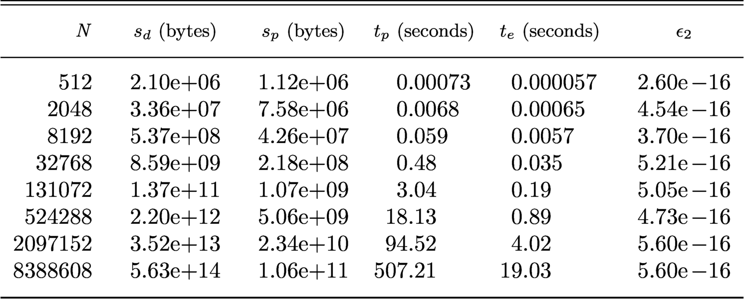
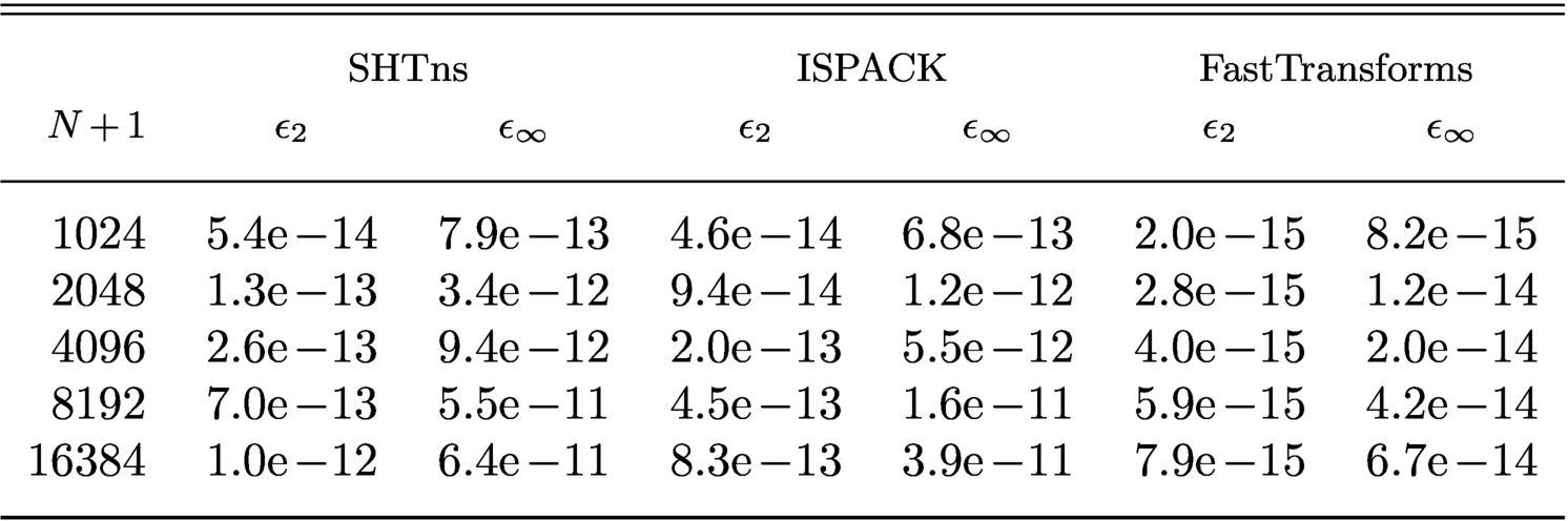
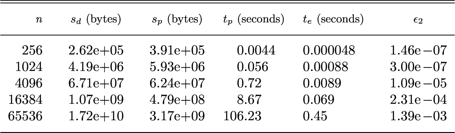
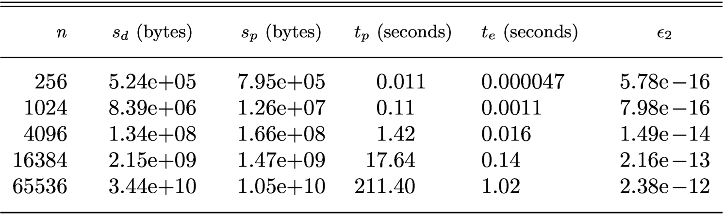
1 Introduction
Orthogonal polynomials (OPs) play a fundamental role in numerical analysis and computational mathematics with applications in quadrature, function approximation and differential equations (Szegő Reference Szegő1975). In the past ten years there has been a resurgence of research attention on the classical properties of orthogonal polynomials, which has led to more efficient algorithms in classical applications as well as new directions. This article aims to give an extensive survey of these recent results. There are three main reasons for the revival of orthogonal polynomials: (1) newfound uses for rigorous asymptotic expansions, (2) the exploitation of sparse and low-rank structure in recurrence relationships, and (3) the introduction of Chebfun, and packages such as ApproxFun and Dedalus, that leverage orthogonal polynomials to automate computations involving functions and differential equations. A general underlying theme is to combine recurrence relationships and asymptotic expansions with structured linear algebra to achieve fast algorithms.
Rigorous asymptotics of special functions is a traditional area of numerical analysis, used to develop trustworthy numerical evaluation schemes for special functions. Two essential types of asymptotic expansions are trigonometric (where a special function is written by a linear combination of cosines and sines) and uniform. The resurgence of interest in these expansions is due to their use in exploiting regions where the special function is trigonometric-like, allowing for a range of fast algorithms based on the fast Fourier transform (FFT) and state-of-the-art numerical linear algebra.
Sparsity in recurrence relationships is also classical, with their use in fast numerical algorithms for differential equations going back to Clenshaw(Reference Clenshaw1957). The success of finite element methods and the development of fast black-box linear algebra reduced their usage. However, OPs have remained popular for computing with functions and solving differential equations on simple geometries (i.e. rectangles, disks, spheres and balls) and in spectral element methods (see Karniadakis and Sherwin Reference Karniadakis and Sherwin2013 for an extensive overview). In particular, they are important in the astrophysics and computational fluid dynamics communities, where simple geometries are prevalent (Burns et al. Reference Burns, Vasil, Oishi, Lecoanet and Brown2020).
The success of software packages such as ApproxFun (Olver, Goretkin, Slevinsky and Townsend Reference Olver, Goretkin, Slevinsky and Townsend2016), Chebfun (Driscoll, Hale and Trefethen Reference Driscoll, Hale and Trefethen2014) and Dedalus (Burns et al. Reference Burns, Vasil, Oishi, Lecoanet and Brown2020) has renewed interest in polynomial approximation and OPs, as the software systems allow one to manipulate functions and accurately solve differential equations with a few lines of Julia, MATLAB and Python code, respectively. These software systems have also led to novel ways to exploit sparsity in the recurrence relationships for OPs. While this survey is primarily on the underlying mathematics, there is a strong link between mathematical research and software design in this subject.
1.1 Outline of paper
Section 2.
We give an overview of univariate and multivariate OPs and their properties, including the classical OPs: Chebyshev, Legendre, ultraspherical, Jacobi, Laguerre and Hermite. Unlike standard introductions, we phrase their construction and properties in terms of quasimatrices. We find this convenient when connecting structured recurrence relationships to structured numerical linear algebra.
Section 3.
We discuss the efficient calculation of quadrature rules using OPs, beginning with the well-known FFT-based algorithms for Clenshaw–Curtis quadrature. We then discuss more recent algorithms for calculating Gauss quadrature rules, building on careful use of asymptotic expansions for calculating the nodes and weights.
Section 4.
We discuss fast transforms for expansions in OPs and spherical harmonics. There are two categories of transforms: transform of coefficients between different families of OPs (e.g. between Chebyshev and Legendre expansions, or between spherical harmonics and tensored Fourier expansions) and transforms between values on a grid and coefficients. The latter typically consists of first converting to a simpler basis using a transform based on the FFT, whereas the former utilizes hidden structure in change-of-basis (connection) matrices.
Section 5.
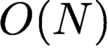
Univariate OPs can be used to transform ordinary differential equations to sparse linear systems using recurrence relationships, facilitating optimal complexity solvers:
 $O(N)$
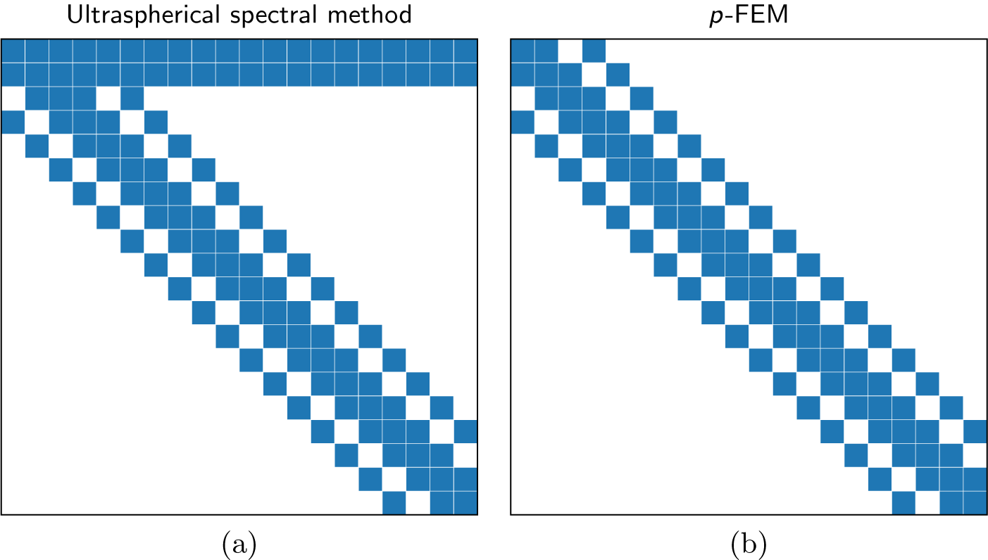
cost for N degrees of freedom. In this vein, we present three methods in a unified framework: integral reformulation as introduced by Clenshaw (Reference Clenshaw1957), the ultraspherical spectral method of Olver and Townsend (Reference Olver and Townsend2013) and a one-dimensional version of the p-finite element method of Shen (Reference Shen1994). Each method has its benefits and trade-offs: integral reformulation is the most straightforward, the ultraspherical spectral method the most versatile. In contrast, the p-finite element method preserves self-adjointness and positive definiteness of the operator. We also discuss domain decomposition, applications to eigenvalue problems and symmetrizing non-symmetric discretizations, which improve the complexity of algorithms for computing eigenvalues.
Section 6.
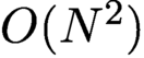
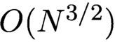
Similarly, multivariate OPs can be used to transform partial differential equations to sparse linear systems. In the case of rectangular geometries this proceeds using a tensor product basis, in which case the sparse linear systems arise from Kronecker products of ordinary differential equations. Naïve direct linear algebra achieves
 $O(N^2)$
complexity for N degrees of freedom. This can be reduced to
 $O({N^{3/2}})$
for operators that can be expressed as a sum of two Kronecker products using the Schur factorization, and improved further to quasi-optimal complexity for the Poisson equation. Going beyond rectangles, the ultraspherical spectral method and p-finite element method have natural extensions to triangles using recurrence relationships, leading to sparse operators. We demonstrate these techniques on simple examples such as the inhomogeneous and variable coefficient Helmholtz equation and the biharmonic equation.
Section 7.
OPs have a natural link to singular integral operators such as the Hilbert, Cauchy/Stieltjes and log-kernel transforms, which can be exploited for the calculation of singular integrals and solution of singular integral equations such as those arising from boundary integral reformulations of partial differential equations. In particular, an ultraspherical-like spectral method is achievable, reducing singular integral equations to sparse linear systems that can be solved efficiently. Low-rank approximation techniques play a role here for handling general kernels.
2 Orthogonal polynomials
A sequence of OPs is a family of polynomials that are orthogonal to each other under some inner product (Szegő Reference Szegő1975). The field of OPs developed from the study of continued fractions, and are now used throughout approximation theory, numerical analysis and computational physics.
2.1 Univariate orthogonal polynomials
Let
 $p_0(x),p_1(x),p_2(x),\ldots $
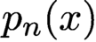
be a sequence of real-valued polynomials such that
 $p_n(x)$
is exactly of degree n, that is,
 $$ \begin{align*} p_n(x) = k_n x^n + O ({x^{n-1}}),\quad k_n \neq 0. \end{align*} $$
We say that
 $p_0(x),p_1(x),p_2(x),\ldots $
are orthogonal polynomials with respect to a non-negative, continuous, weight function w over a (possibly infinite) interval
 $(a,b)$
if
 $$ \begin{align} \langle p_m,p_n\rangle_w = \int_a^b w(x) p_m(x) p_n(x) {{\mathrm{d}}x} = \begin{cases} 0 &m\neq n,\\ h_n & m= n. \end{cases} \end{align} $$
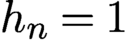
If
 $h_n=1$
, then the polynomials are not just orthogonal but orthonormal. Given a weight function, the orthonormal polynomials associated with w are unique up-to-sign.
Any set of OPs can be rescaled to be orthonormal; however, the standard normalizations (Szegő Reference Szegő1975) are determined by prescribing their values at special points. With the standard definitions, classical OPs have simple rational recurrence relationships that are extremely efficient to generate, whereas their normalized counterparts involve square roots. In practical computations, this is typically helpful, though we deviate from this convention for legitimate reasons from time to time.
2.2 Quasimatrix notation and orthogonal polynomial expansions
Many applications of OPs use them as a convenient basis in which to represent functions. Let
 $p_0(x),p_1(x),p_2(x),\ldots $
be a sequence of univariate OPs on
 $[a,b]$
with respect to the weight function w; then
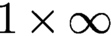
 $$ \begin{align*} f(x) = \sum_{n=0}^\infty p_n(x) f_n = \boldsymbol{P}(x)\boldsymbol{f}, \quad \boldsymbol{P}(x) = (p_0(x)\mid p_1(x) \mid \cdots), \end{align*} $$
where
 $\boldsymbol {f} = (f_0,f_1,\ldots )^{\top }$
is an infinite vector and
 $\boldsymbol {P}(x)$
is a
 $1 \times \infty $
row-vector.
We view
 $\boldsymbol {P}$
as an
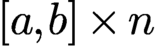
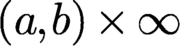 $(a,b)\times \infty $
quasimatrix,Footnote
1
a formalism that allows us to view it as a linear map from coefficients to functions. That is, we can view
 $\boldsymbol {P}$
as the synthesis operator: a one-to-one linear map from the space of infinite vectors with a finite number of non-zero entries (
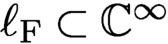 $\ell _{\mathrm F} \subset {\mathbb C}^\infty $
) to the space of polynomials (
 ${\mathbb C}[x]$
). Of course, we can go further and relate other coefficient spaces to function spaces (e.g. with Legendre polynomials it is a one-to-one map from
 $\ell ^2$
to
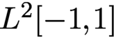 $L^2[-1,1]$
) and quasimatrices allow us to discuss these maps collectively, but for our discussion it suffices to interpret the map as
 $\boldsymbol {P} \colon \ell _{\mathrm F} \rightarrow {\mathbb C}[x]$
. We take the convention that
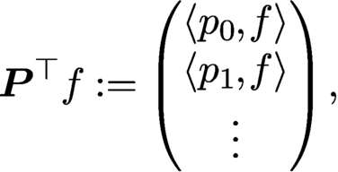 $$ \begin{align*} \boldsymbol{P}^\top f := \begin{pmatrix} {\langle p_0,f\rangle}\\ {\langle p_1,f\rangle}\\ \vdots\end{pmatrix}, \end{align*} $$
where
 $\langle \cdot ,\cdot \rangle $
is the
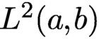 $L^2(a,b)$
inner product. We therefore have the analysis operator
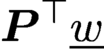 $\boldsymbol {P}^\top \underline w$
, where the underbar indicates that it is the multiplication by w operator. That is,
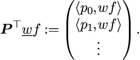 $$ \begin{align*} \boldsymbol{P}^\top \underline w f := \begin{pmatrix} {\langle p_0,w f\rangle}\\ {\langle p_1,w f\rangle}\\ \vdots\end{pmatrix}. \end{align*} $$
Given a polynomial
 $f(x)$
we can solve the following linear system:
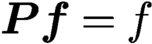 $$ \begin{align*} \boldsymbol{P}\boldsymbol{f} = f \end{align*} $$
for the expansion coefficients,
 $\boldsymbol {f}$
. Due to the orthogonality, we find that
 $$ \begin{align*} \boldsymbol{P}^\top \underline w \boldsymbol{P} = D_{\boldsymbol{h}} = \mathrm{diag}( h_0, h_1,\dots ), \end{align*} $$
where
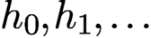 $h_0,h_1,\ldots $
are the orthogonality constants in (2.1). This means that
 $$ \begin{align*} \boldsymbol{f} = \boldsymbol{P}^{-1} f = (\boldsymbol{P}^\top \underline w \boldsymbol{P} )^{-1} \boldsymbol{P}^\top \underline w f = D_{\boldsymbol{h}}^{-1}\boldsymbol{P}^\top \underline w f . \end{align*} $$
Equivalently, for
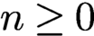 $n \geq 0$
, we have
 $$ \begin{align} f_n = \dfrac{1}{h_n}\int_a^b p_n(x) w(x) f(x){{\mathrm{d}}x}, \quad h_n = \int_a^b w(x)(p_n(x))^2 {{\mathrm{d}}x}. \end{align} $$
Due to the orthogonality of
 $p_0,p_1,\ldots $
the coefficient
 $f_n$
can be computed independently of the other entries of
 $\boldsymbol {f}$
.
For non-polynomial functions f, one needs to use truncated orthogonal polynomial expansions to approximate f. In particular, if f is a sufficiently smooth function on
 $[a,b]$
, then one expects that the entries in
 $\boldsymbol {f}$
decay to zero. The expansion can be truncated after N terms to obtain a polynomial approximation to f,
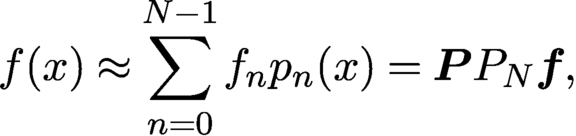 $$ \begin{align*} f(x) \approx \sum_{n=0}^{N-1} f_n p_n(x) = \boldsymbol{P} P_N \boldsymbol{f}, \end{align*} $$
where
 $P_N \boldsymbol {f} = (f_0,\ldots ,f_{N-1},0,0,\ldots )^{\top }$
is the truncation operator
 $P_N \colon {\mathbb C}^\infty \rightarrow \ell _{\mathcal F}$
. A polynomial approximation to f, formed in this way, can serve as a proxy to f and make subsequent computations more efficient (Boyd Reference Boyd2013). In principle, to compute a polynomial approximation to f, the coefficients
 $f_n$
for
 $0\leq n\leq N-1$
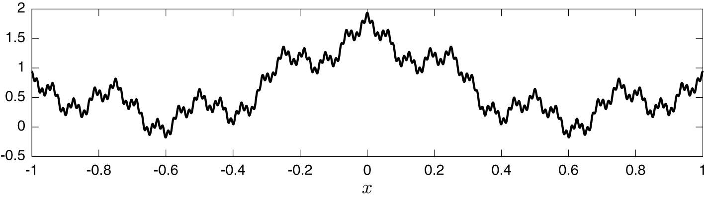
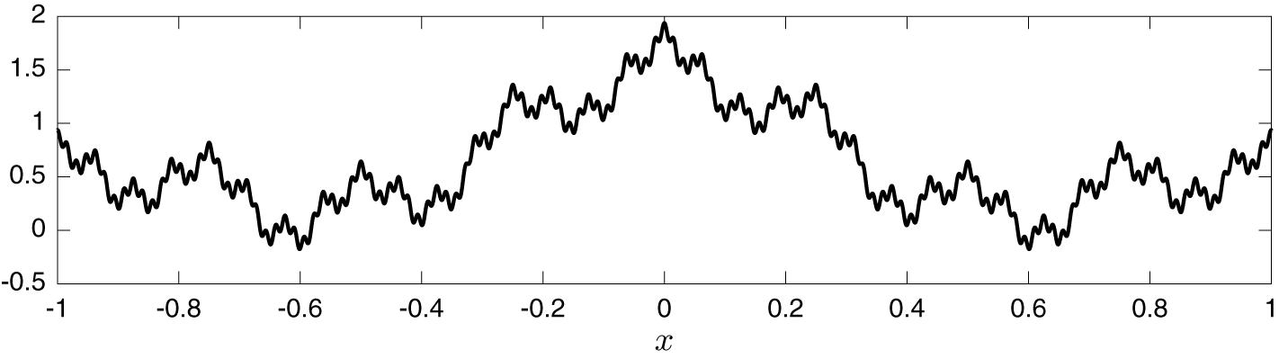
need to be computed via the integral expression in (2.2). However, this is computationally prohibitive for large N. Instead, fast transformation from samples of f to expansion coefficients are desirable (see Section 4). In Figure 2.1 we show a function approximated by a finite Chebyshev expansion. The degree of the polynomial used to represent this function was adaptively selected using the effective heuristic of Aurentz and Trefethen (Reference Aurentz and Trefethen2017).
The function
 $f(x) = \sum _{k=0}^5 2^{-k} \cos (({\pi }/{2})4^kx)$
approximated by a polynomial of degree
 $476$
to within machine precision, where the polynomial is represented using a Chebyshev expansion.
Quasimatrices provide convenient notation for representing the action of continuous operators by discrete operators. For example, consider the quasimatrix formed by the monomials
 $\boldsymbol {Z}(z) = (1| z\mid z^2\mid \cdots )$
defined on the unit disk. A simple relationship for differentiation is
 $$ \begin{align} {\mathcal D} \boldsymbol{Z}(z) = (0\ \mid\ 1\ \mid \ 2 z\ \mid \ 3 z^2\ \mid\ \cdots ] = \boldsymbol{Z}(z) \begin{pmatrix}0 & 1 \\ && 2 \\ &&& \ddots \end{pmatrix}\!, \end{align} $$
where
 ${\mathcal D}$
is the differentiation operator. This is clearly true when viewing this as an operator
 ${\mathcal D} \boldsymbol {Z} \colon \ell _F \rightarrow {\mathbb C}[z]$
, with suitable extensions to sufficiently fast decaying coefficient spaces.
Remark 2.1. In what follows, we use quasimatrices without being specific about the spaces they act on. We note that it is usually straightforward to deduce these from the actual entries of the resulting operators. For example, for monomials, we have
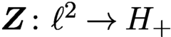 $\boldsymbol {Z} \colon \ell ^2 \rightarrow H_+$
, where
 $H_+$
is the Hardy space on the unit circle. One can also see from the growth in the operator in (2.3) that
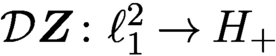 ${\mathcal D} \boldsymbol {Z} \colon \ell _1^2 \rightarrow H_+$
is bounded, where
 $$ \begin{align*} \ell_1^2 = \biggl\{{ \boldsymbol{f} } \in \mathbb{C}^{\infty} \colon \sum_{n=0}^ \infty ((n+1) \boldsymbol{f} _n)^2 < \infty \biggr\}. \end{align*} $$
That is, one can combine known relationships between spaces coming from approximation theory with trivial relationships deduced from the growth properties of banded operators to deduce precise statements.
2.3 The Jacobi operator associated to orthogonal polynomials
All sets of orthogonal univariate polynomials satisfy a three-term recurrence relationship. That is, all univariate OPs satisfy a recurrence of the form
 $$ \begin{align} xp_n(x) &= c_np_{n-1}(x) + a_n p_n(x) + b_n p_{n+1}(x), \quad n\geq 1, \end{align} $$
 $$ \begin{align} xp_0(x) &= a_0p_0(x) + b_0p_1(x). \end{align} $$
One of the simplest ways to evaluate
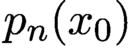 $p_n(x_0)$
at a point
 $x_0$
is to use the three-term recurrence (perhaps with some care) to successively evaluate
 $p_0(x_0),\ldots ,p_{n-1}(x_0)$
, before finally computing
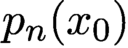 $p_n(x_0)$
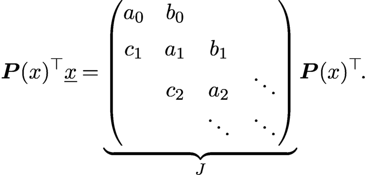
(Gautschi Reference Gautschi1967). The recurrence in (2.5) can be encoded as a tridiagonal operator, known as a (non-symmetric) Jacobi operator.
Definition 2.2. A (non-symmetric) Jacobi operator, J, associated with a family of OPs is the tridiagonal operator given by
 $$ \begin{align} \boldsymbol{P}(x)^{\top} \underline{x} = \underbrace{\begin{pmatrix}a_0 & b_0 \\[5pt] c_1 & a_1 & b_1 \\ & c_2 & a_2 & \ddots \\ &&\ddots & \ddots\end{pmatrix}}_{J} {\boldsymbol{P}}(x)^\top\!. \end{align} $$
If the family of OPs are orthonormal, then J is a symmetric tridiagonal operator (Gautschi Reference Gautschi2004).
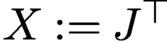
The transpose of a Jacobi operator, denoted by
 $X := J^\top $
, is the discrete operator that represents multiplication by x in the OP basis. This can be seen from (2.5) by transposing (2.6) to obtain the relationship
 $x {\boldsymbol {P}} = {\boldsymbol {P}} X$
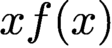
. That means that if
 $f(x) = \boldsymbol {P}(x) \boldsymbol {f}$
, then the expansion coefficients of
 $xf(x)$
are
 $X \boldsymbol {f}$
, that is,
 $$ \begin{align*} xf(x) = x\boldsymbol{P}(x) \boldsymbol{f} = \boldsymbol{P}(x) X \boldsymbol{f}. \end{align*} $$
To multiply a function f expressed in an OP expansion by x, we can apply the operator X to the expansion coefficients of f.
2.4 Classical univariate orthogonal polynomials
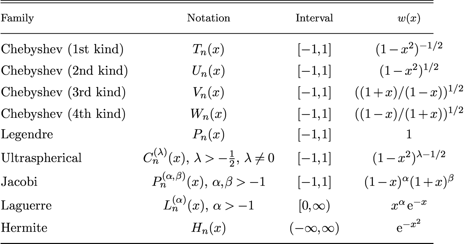
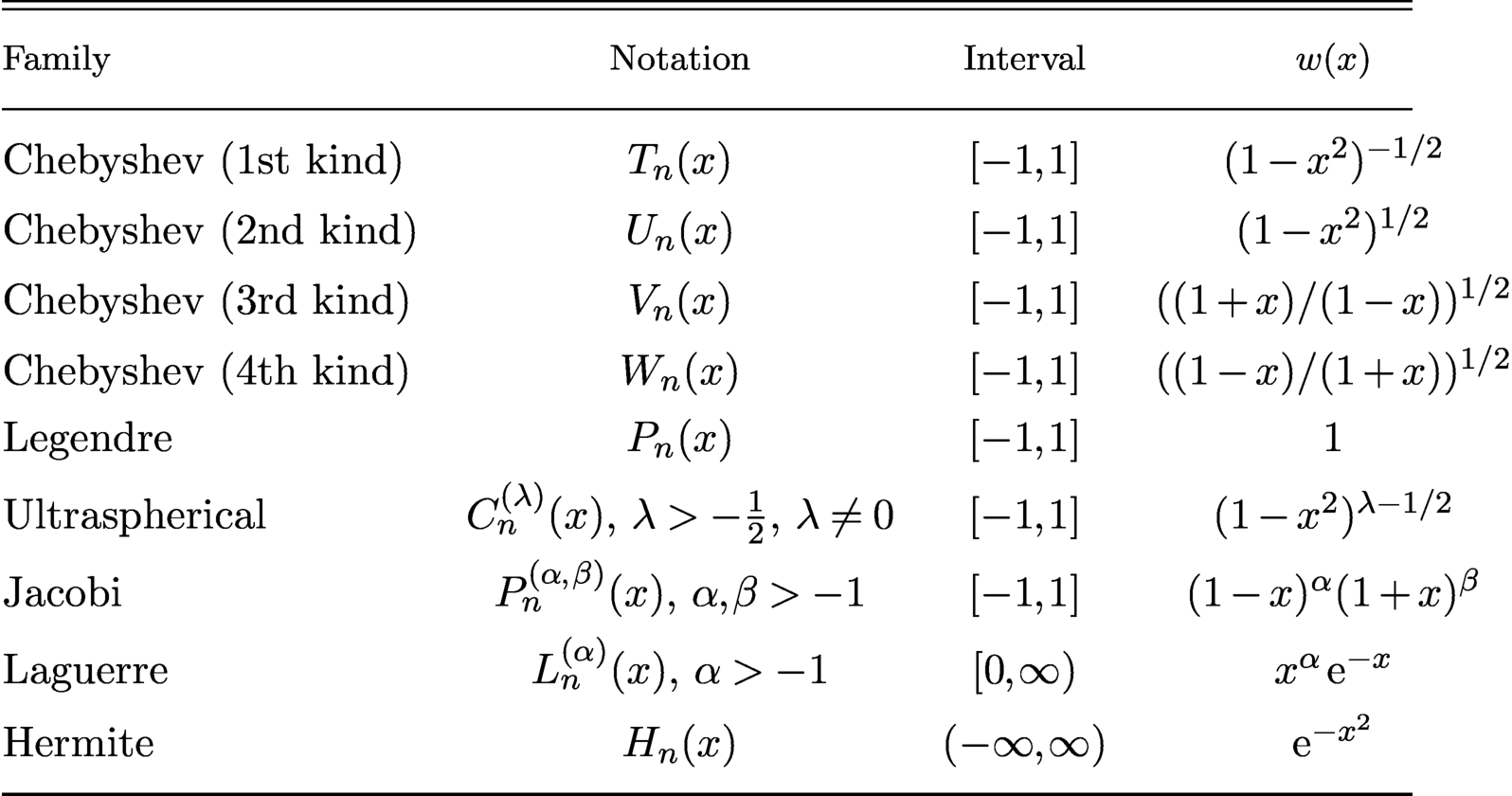
Classical OPs are the most widely used univariate OPs and consist of Hermite polynomials, generalized Laguerre polynomials and Jacobi polynomials (including as special cases the ultraspherical, Chebyshev and Legendre polynomials). These polynomials have several characterizing properties that make them computationally useful and single them out from other OPs: (1) they are the only univariate OPs (up to a linear change of variables) whose derivatives are also OPs (Sonine Reference Sonine1887), and (2) they satisfy a fixed second-order Sturm–Liouville differential equation. The first property makes them ideal in spectral methods for solving differential equations, while (2) ensures that there are asymptotic expansions that hold for the entire family of OPs. Table 2.1 details the classical OPs, along with their orthogonality.
The classical OPs on bounded and unbounded real intervals. Up to a linear change of variables, the classical OPs are the only univariate OPs whose derivatives are also OPs.
The Jacobi polynomials
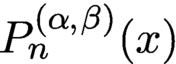 $P_n^{(\alpha ,\beta )}(x)$
are orthogonal with respect to the weight function
 $w(x) = (1-x)^\alpha (1+x)^\beta $
with
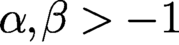 $\alpha ,\beta>-1$
and are scaled so that
 $$ \begin{align*} P_n^{(\alpha,\beta)}(x) = \dfrac{(n+\alpha+\beta+1)_n}{2^n n!} x^n + \cdots, \end{align*} $$
where
 $(\alpha )_\beta $
is the Pochhammer symbol. They are useful special functions for singular integral equations, quadrature rules, building multivariable OPs, and random matrix theory. In quasimatrix notation, we may write
 $$ \begin{align*} {\boldsymbol{P}}^{(\alpha,\beta)}(x) := \bigl(P_0^{(\alpha,\beta)}(x)\mid P_1^{(\alpha,\beta)}(x)\mid \cdots\bigr). \end{align*} $$
Special cases of Jacobi polynomials include ultraspherical
 $$ \begin{align*} C_n^{(\lambda)}(x) = (2\lambda)_n/(\lambda+1/2)_nP_n^{(\lambda-1/2,\lambda-1/2)}(x), \end{align*} $$
Legendre
 $P_n(x) = P^{(0,0)}_n(x)$
, and Chebyshev polynomials (four kinds):Footnote
2
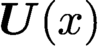
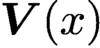
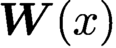
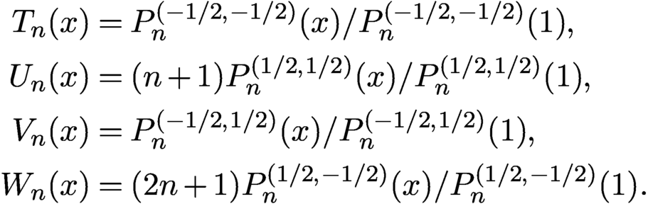 $$ \begin{align*} T_n(x) & = P_n^{(-{1}/{2},-{1}/{2})}(x)/P_n^{(-{1}/{2},-{1}/{2})}(1),\\ U_n(x) & = (n+1) P_n^{({1}/{2},{1}/{2})}(x)/P_n^{({1}/{2},{1}/{2})}(1),\\ V_n(x) & = P_n^{(-{1}/{2},{1}/{2})}(x)/P_n^{(-{1}/{2},{1}/{2})}(1),\\ W_n(x) & = (2n+1) P_n^{({1}/{2},-{1}/{2})}(x)/P_n^{({1}/{2},-{1}/{2})}(1). \end{align*} $$
Associated to these OPs are the quasimatrices
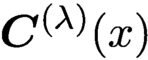 $\boldsymbol {C}^{(\lambda )}(x)$
,
 $\boldsymbol {P}(x)$
,
 $\boldsymbol {T}(x)$
,
 $\boldsymbol {U}(x)$
,
 $\boldsymbol {V}(x)$
and
 $\boldsymbol {W}(x)$
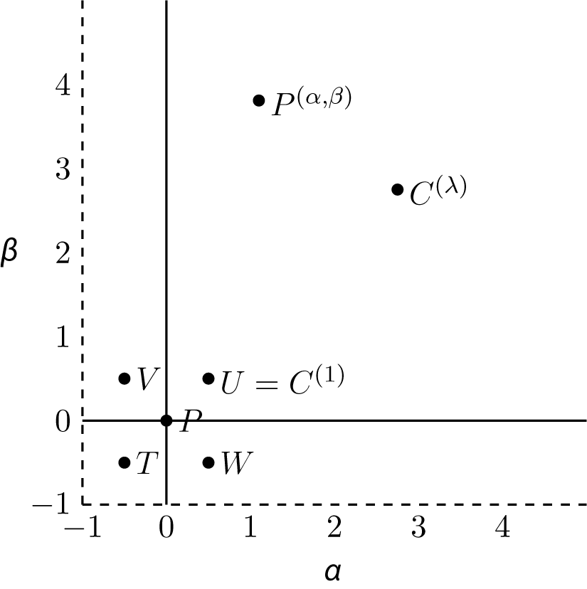
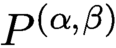
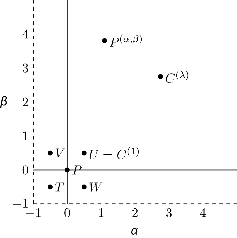
, respectively. Figure 2.2 summarizes the special cases of Jacobi polynomials. The figure is useful for understanding and exploring sparse recurrence relationships for derivatives, weighted derivatives and change-of-basis (conversion) operators.
Jacobi polynomials
 $P^{(\alpha ,\beta )}$
for
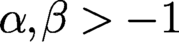 $\alpha ,\beta>-1$
are orthogonal with respect to
 $w(x) = (1-x)^\alpha (1+x)^\beta $
. Along the diagonal
 $\alpha =\beta = \lambda -1/2$
the OPs are referred to as ultraspherical polynomials and are denoted by
 $C^{(\lambda )}$
for
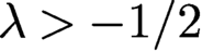 $\lambda> -{1}/{2}$
,
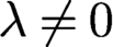 $\lambda \ne 0$
.
2.5 Multivariate orthogonal polynomials
OPs are also possible in multiple variables, and Dunkl and Xu (Reference Dunkl and Xu2014) give a comprehensive overview. For a multi-index
 $\alpha = (\alpha _1,\ldots ,\alpha _d)\in \mathbb {N}_0^d$
, where
 $\mathbb {N}_0 = \{0, 1, 2, \ldots \}$
, and
 $\mathbf {x} = (x_1,\ldots ,x_d)$
, a monomial term is given by
 $\mathbf {x}^\alpha = x_1^{\alpha _1}\cdots x_d^{\alpha _d}$
. The number
 $|\alpha | = \alpha _1 + \cdots + \alpha _d$
is called the (total) degree of
 $\mathbf {x}^\alpha $
. The space of polynomials of (total) degree at most n is denoted by
 $$ \begin{align*} \Pi_n^d = \operatorname{Span} \{\mathbf{x}^\alpha \colon |\alpha|\leq n, \alpha \in \mathbb{N}_0^d \}. \end{align*} $$
A polynomial
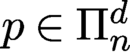 $p\in \Pi _n^d$
is said to be an orthogonal polynomial of degree n with respect to a weight function
 $w(\boldsymbol {x})$
if
 $$ \begin{align*} \int\!\!\cdots\!\!\int p(\boldsymbol{x}) w(\boldsymbol{x}) q(\boldsymbol{x}) {\mathrm{d}} \boldsymbol{x} = 0 \end{align*} $$
for any
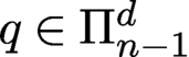 $q\in \Pi _{n-1}^d$
. This means that p is orthogonal to all polynomials of lower degree, though it does not have to be orthogonal to polynomials of the same degree. We will only use mutually orthogonal polynomials which are also orthogonal with polynomials of the same degree.
We find it convenient to express a family of multivariable OPs as a block-quasimatrix, where each block contains the polynomials of the same total degree. In two variables we write
 $$ \begin{align*} \boldsymbol{P}(\boldsymbol{x}) = (p_{00}(\boldsymbol{x}) \mid {p_{10}(\boldsymbol{x}) \mid p_{11}(\boldsymbol{x})} \mid {p_{20}(\boldsymbol{x}) \mid p_{21}(\boldsymbol{x}) \mid p_{22}(\boldsymbol{x})} \mid \cdots ), \end{align*} $$
while in three variables we have
 $$ \begin{align*} \boldsymbol{P}(\boldsymbol{x}) = (p_{00}(\boldsymbol{x}) \mid {p_{10}(\boldsymbol{x}) \mid p_{11}(\boldsymbol{x}) \mid p_{12}(\boldsymbol{x})} \mid \cdots ). \end{align*} $$
A sequence of multivariable OPs is said to be orthonormal with respect to w if all the polynomials of a given degree are orthogonal and of unit length, i.e.
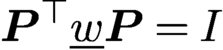 $\boldsymbol {P}^\top \underline w \boldsymbol {P} = I$
, where I is the identity operator. OPs in multiple variable are only unique up to an orthogonal recombination. In two variables, given any sequence of
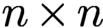 $n\times n$
orthogonal matrices
 $Q_n$
, we find that if
 $\boldsymbol {P}$
are orthonormal then
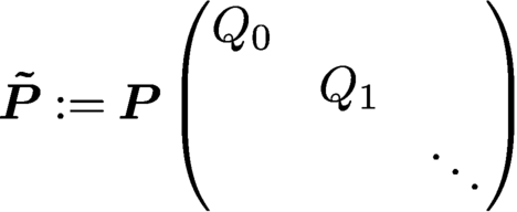 $$ \begin{align*} \boldsymbol{\tilde P} := \boldsymbol{P} \begin{pmatrix}Q_0 \\ &Q_1 \\ && \ddots\end{pmatrix} \end{align*} $$
is also orthonormal with respect to the same weight, since
 $$ \begin{align*} \boldsymbol{\tilde P}^{\top} \underline w \boldsymbol{\tilde P} = \begin{pmatrix}Q_0^{\top} \\ &Q_1^{\top} \\ && \ddots\end{pmatrix} \boldsymbol{P}^{\top} \underline w \boldsymbol{P} \begin{pmatrix}Q_0 \\ &Q_1 \\ && \ddots\end{pmatrix} = I. \end{align*} $$
Therefore, the choice of basis in multivariable OPs is always somewhat arbitrary, though different choices lead to different sparsity properties in recurrence relationships.
Multivariable OPs satisfy a three-term recurrence relationship in each variable and hence have an associated (non-symmetric) Jacobi operator for each variable.
Definition 2.3. The Jacobi operators
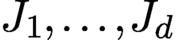 $J_1, \ldots , J_d$
associated with a family of multivariate OPs are block-tridiagonal operators such that
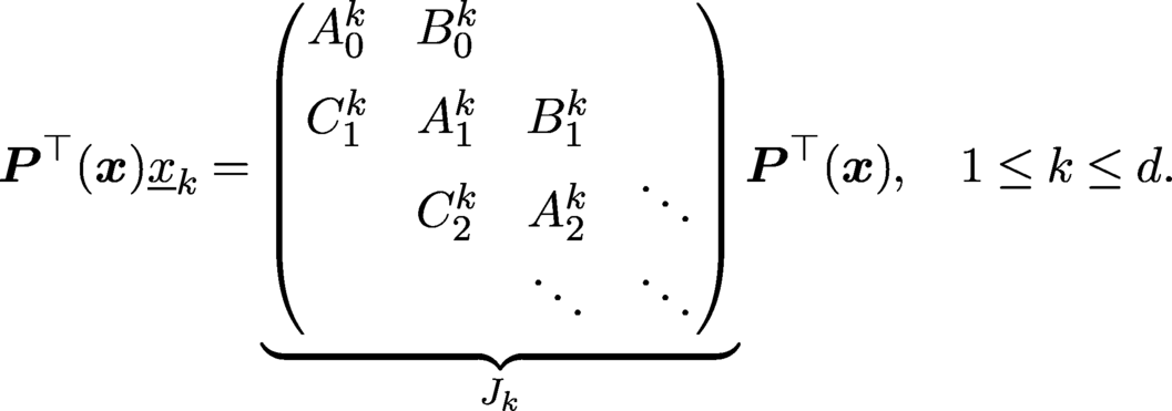 $$ \begin{align*} {\boldsymbol{P}}^{\top} (\boldsymbol{x}) \underline x_k = \underbrace{ \begin{pmatrix}A_0^k & B_0^k \\[6pt] C_1^k & A_1^k & B_1^k \\ & C_2^k & A_2^k & \ddots \\ &&\ddots & \ddots\end{pmatrix}}_{J_k} {\boldsymbol{P}}^{\top} (\boldsymbol{x}), \quad 1\leq k \leq d. \end{align*} $$
The sizes of
 $A_n^k$
,
 $B_n^k$
and
 $C_n^k$
are determined by the number of ways d non-negative integers can be chosen to sum to k. When
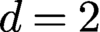 $d = 2$
, we have
 $A_n^k \in {\mathbb R}^{(n+1) \times (n+1)}$
,
 $B_n^k \in {\mathbb R}^{(n+1) \times (n+2)}$
and
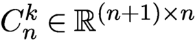 $C_n^k \in {\mathbb R}^{(n+1) \times n}$
.
Again, the transpose of
 $J_k$
for
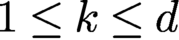 $1\leq k\leq d$
, denoted by
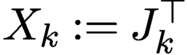 $X_k := J_k^{\top }$
, is the discrete operator that represents multiplication by
 $x_k$
in the OP basis. That is, if
 $f(\boldsymbol {x}) = \boldsymbol {P}(\boldsymbol {x})\boldsymbol {f}$
, then the expansion coefficients for
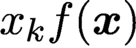 $x_kf(\boldsymbol {x})$
are
 $X_k \boldsymbol {f}$
, since
 $$ \begin{align*} x_kf(\boldsymbol{x}) = x_k\boldsymbol{P}(\boldsymbol{x})\boldsymbol{f} = \boldsymbol{P}(\boldsymbol{x}) X_k \boldsymbol{f}. \end{align*} $$
If the family of OPs are orthonormal, then
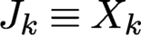 $J_k \equiv X_k$
is symmetric, that is,
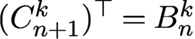 $(C_{n+1}^k)^{\top } = B_n^k$
and
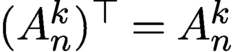 $(A_n^k)^{\top } = A_n^k$
for
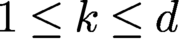 $1\leq k\leq d$
and
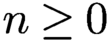 $n\geq 0$
.
2.6 Constructing multivariate orthogonal polynomials
Classical multivariate OPs are defined on simple geometries such as rectangles, disks, triangles, hypercubes, balls and tetrahedra. There are, at least, two advantages to constructing multivariate OPs from univariate ones: (1) they typically have simple expressions in terms of univariate OPs, and (2) recurrence relationships can be derived from known univariate relationships. Two useful ways to construct multivariate OPs are tensor products and Koornwinder’s construction (Koornwinder Reference Koornwinder and Askey1975).
2.6.1 Tensor product construction
OPs on tensor product domains (e.g. squares and hypercubes) can be constructed using the tensor product of univariate OPs. If
 $\phi _0(x),\phi _1(x),\ldots $
and
 $\psi _0(x),\psi _1(x),\ldots $
are two sequences of OPs with respect to the weight
 $w_1$
on
 $[a,b]$
and
 $w_2$
on
 $[c,d]$
, then
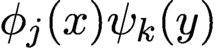 $\phi _j(x)\psi _k(y)$
for
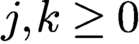 $j,k\geq 0$
are orthogonal with weight
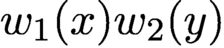 $w_1(x)w_2(y)$
on
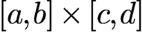 $[a,b]\times [c,d]$
. Let
 ${\boldsymbol {\Phi }}(x) = (\phi _0(x) \mid \phi _1(x) \mid \cdots )$
and
 ${\boldsymbol {\Psi }}(x) = (\psi _0(x) \mid \psi _1(x) \mid \cdots )$
. Then in terms of quasimatrices we can define the tensor product
 $ {\boldsymbol {\Phi }} \otimes {\boldsymbol {\Psi }}$
as a generalization of a quasimatrix defined on
 ${\mathbb R}^2$
:
 $$ \begin{align*} ({\boldsymbol{\Phi}} \otimes {\boldsymbol{\Psi}})_{j,k}(x,y) = \phi_j(x) \psi_k(y), \quad j,k\geq 0. \end{align*} $$
One could then express coefficients as a matrix with multiplication defined tensor-wise. That is, if
 $F \in {\mathbb C}^\infty \otimes {\mathbb C}^\infty $
we would (formally) have
 $$ \begin{align*} f(x,y) = ({\boldsymbol{\Phi}} \otimes {\boldsymbol{\Psi}})(x,y) F, \end{align*} $$
thus we can view
 ${\boldsymbol {\Phi }} \otimes {\boldsymbol {\Psi }} \colon \ell _{\mathcal F}^2 \rightarrow {\mathbb C}[x,y]$
, where
 $\ell _{\mathcal F}^2$
denotes the space of matrices with finite number of non-zero entries.
It is often convenient to identify
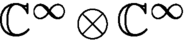 ${\mathbb C}^\infty \otimes {\mathbb C}^\infty $
with infinite matrices
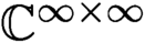 ${\mathbb C}^{\infty \times \infty }$
, in which case we write
 $$ \begin{align*} f(x,y) = \sum_{j,k=0}^\infty F_{j,k} \phi_j(x) \psi_k(y), = {\boldsymbol{\Phi}}(x) F {\boldsymbol{\Psi}}(y)^{\top}. \end{align*} $$
One still needs to determine how the entries of F are stored sequentially in memory. A natural approach is to replace the infinite matrix F with an
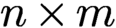 $n \times m$
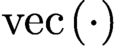
truncation and order the entries column by column (column major) or row by row (row major), with column major being the modern standard. We can interpret this as a block-quasimatrix, with blocks of size n, and denote it by
 ${\text {vec}\,}(\cdot )$
as follows:
 $$ \begin{align*} &{\text{vec}\,}(\Phi_n \otimes \Psi_m)(x,y) \\[2pt] &\quad := ({\phi_0(x)\psi_0(y) ,\ldots, \phi_n(x)\psi_0(y)} \mid \cdots \mid {\phi_0(x)\psi_m(y) ,\ldots, \phi_n(x)\psi_m(y)}). \end{align*} $$
This point of view is computationally convenient for OPs on tensor product domains when working with truncated expansions, and naturally leads to the discretization of certain partial differential equations as generalized Sylvester equations (see Section 6.2).
An alternative viewpoint is to traverse the basis in an anti-diagonal way:
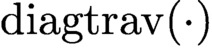
 $$ \begin{align*} \boldsymbol{P}(x,y) & = \operatorname{diagtrav} ( {\boldsymbol{\Phi}}(x) \otimes {\boldsymbol{\Psi}}(y) ) \\[2pt] & = (\phi_0(x) \psi_0(y) \ \mid {\phi_1(x) \psi_0(y) \mid \phi_0(x) \psi_1(y)} \mid \cdots ). \end{align*} $$
That is,
 $\operatorname {diagtrav} (\cdot )$
traverses a square infinite matrix and writes it out in anti-diagonal order. This has the benefit of grouping coefficients in blocks of polynomial degree, which fits the definition of multivariate OPs and extends naturally to non-tensor domains.
Remark 2.4. Another basis ordering is the hyperbolic cross, which comes up in high-dimensional quadrature to circumvent the curse of dimensionality. We focus on low-dimensional settings, where these are less useful.
2.6.2 Koornwinder’s construction
Another construction of multivariate OPs is given by Koornwinder (Reference Koornwinder and Askey1975). Let
 $w_1$
and
 $w_2$
be weight functions on
 $[a,b]$
and
 $[c,d]$
, respectively, and let
 $\rho (x)$
be a function on
 $(a,b)$
such that either
-
(1)
 $\rho $
is a polynomial of degree
$1$
, or
-
(2)
$\rho ^2$
is non-negative polynomial of degree
$\leq 2$
with
$c = -d>0$
and
$w_2$
is an even function.




Then one can construct multivariate OPs with respect to the weight function
 $W(x,y) = w_1(x) w_2( y /\rho (x) )$
on
 $\Omega = \{(x,y) \colon c\rho (x)\leq y \leq d\rho (x), a\leq x\leq b\}$
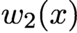
. To form the multivariate OPs, first write down all the univariate OPs
 $p_{0}^{(k)}(x),p_{1}^{(k)}(x),\ldots ,$
associated to
 $\rho ^{2k+1}(x)w_1(x)$
on
 $[a,b]$
and the univariate OPs
 $q_0(x),q_1(x),\ldots ,$
associated to
 $w_2(x)$
on
 $[c,d]$
. It can be shown that the bivariate polynomials given by
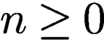
 $$ \begin{align*} P_{n,k}(x,y) = p_{n-k}^{(k)}(x) {\rho(x)^k} q_k( y/\rho(x) ), \quad 0\leq k\leq n, \end{align*} $$
for each
 $n\geq 0$
are OPs on
 $\Omega $
with respect to
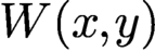 $W(x,y)$
(Dunkl and Xu Reference Dunkl and Xu2014). Note that there are natural extensions to higher dimensions, as outlined in Dunkl and Xu (Reference Dunkl and Xu2014).
In the degenerate case,
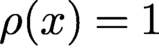 $\rho (x) = 1$
, the construction derives tensor product OPs for tensor product domains. However, the non-degenerate cases include OPs on spheres, disks, triangles and more exotic domains.
‘Legendre’ polynomials on a right-angled triangle.
Let
 $$ \begin{align*} \Omega = \{(x,y) \colon 0\leq y\leq x, 0\leq x\leq 1\} \end{align*} $$
be a right-angled triangle. Using Koornwinder’s construction with
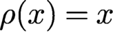 $\rho (x) = x$
and
 $w_1(x) = w_2(x) = 1$
, we find that
 $$ \begin{align*} {P_{n,k}}(x,y) = P_{n-k}^{(2k+1,0)}(2x-1) x^k P_k\biggl(2\displaystyle \frac{y}{x}-1\biggr), \quad 0\leq k\leq n, \ n\geq 0, \end{align*} $$
are OPs on the right-angled triangle with
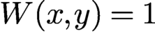 $W(x,y) = 1$
.
‘Jacobi’ polynomials on a right-angled triangle.
Let
 $$ \begin{align*} \Omega = \{(x,y) \colon 0\leq y\leq x, 0\leq x\leq 1\} \end{align*} $$
be a right-angled triangle. Letting
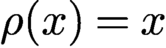 $\rho (x) = x$
,
 $w_1(x) = x^a(1-x)^b$
and
 $w_2(x) = x^c(1-x)^d$
, with
 $a,b,c,d>-1$
, we find that
 $$ \begin{align*} {P_{n,k}^{(a,b,c,d)}}(x,y) = P_{n-k}^{(2k+a+1,b)}(2x-1) x^k P_k^{(c,d)}\biggl(2\displaystyle \frac{y}{x}-1\biggr), \quad 0\leq k\leq n, \ n\geq 0, \end{align*} $$
are OPs on the right-angled triangle with respect to
 $W(x,y) = x^a(1-x)^b(y/x)^c(1-y/x)^d$
. An affine translation of this construction and setting
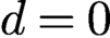 $d = 0$
gives the standard Jacobi polynomials on the unit simplex
 $0 \leq x \leq 1, 0 \leq y \leq 1-x$
, which are orthogonal with respect to
 $x^a y^b (1-x-y)^c$
:
 $$ \begin{align*} P_{n,k}^{(a,b,c)}(x,y) = P_{n-k}^{(2k+b+c+1,a)}(2x-1) (1-x)^k P_k^{(b,c)}\biggl(2\displaystyle \frac{y}{1-x}-1\biggr). \end{align*} $$
‘Legendre’ polynomials on the unit disk.
The unit disk can be described as
 $$ \begin{align*} \Omega = \{(x,y) \colon -\rho(x) \leq y\leq \rho(x), -1\leq x\leq 1\}, \end{align*} $$
where
 $\rho (x) = \sqrt {1-x^2}$
. Following Koornwinder’s construction with
 $w_1(x) = w_2(x) = 1$
, we find that
 $$ \begin{align*} Z_{n,k}(x,y) = C_{n-k}^{(k+1)}(x) (1-x^2)^{k/2} P_k\biggl(\displaystyle \frac{y}{\sqrt{1-x^2}}\biggr), \quad 0\leq k\leq n, \ n\geq 0, \end{align*} $$
are OPs on the unit disk with
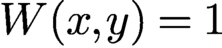 $W(x,y) = 1$
.
Alternatively, it is common to use polar coordinates on the disk so that
 $$ \begin{align*} Z_{n,k}(r,\theta) = P_{{(n-|k|)}/{2}}^{(0,|k|)}(2r^2-1) r^{|k|} \,{\mathrm{e}}^{{\mathrm i} k\theta}, \quad -n\leq k\leq n, \ n\geq 0, \end{align*} $$
where
 $n-k$
is even. These polynomials are also referred to as the Zernike polynomials (Zernike Reference Zernike1934).
‘Ultraspherical’ polynomials on the unit disk.
The unit disk can be described as
 $$ \begin{align*} \Omega = \{(x,y) \colon -\rho(x) \leq y\leq \rho(x), -1\leq x\leq 1\}, \end{align*} $$
where
 $\rho (x) = \sqrt {1-x^2}$
. Following Koornwinder’s construction with
 $w_1(x) = w_2(x) = (1-x^2)^{\lambda -1/2}$
, we find that
 $$ \begin{align*} Z_{n,k}^{(\lambda)}(x,y) = C_{n-k}^{(k+1)}(x) (1-x^2)^{k/2} C_k^{(\lambda)}\biggl(\displaystyle \frac{y}{\sqrt{1-x^2}}\biggr), \quad 0\leq k\leq n, \ n\geq 0, \end{align*} $$
are OPs on the unit disk with
 $W(x,y) = (1-\|x \|^2)^\lambda $
.
And on the unit sphere
 $$ \begin{align*} \Omega = \{(x,y,z)\in{\mathbb R}^3 \colon x^2+y^2+z^2 = 1\}, \end{align*} $$
parametrized by co-latitude
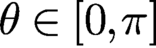 $\theta \in [0,\pi ]$
and longitude
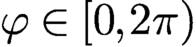 $\varphi \in [0,2\pi )$
, spherical harmonics (Atkinson and Han Reference Atkinson and Han2012, Dai and Xu Reference Dai and Xu2013) share a similar structural property with Koornwinder’s constructions and the periodic representation of Zernike polynomials
 $$ \begin{align*} Y_n^k(\theta,\varphi) = P_{n-|k|}^{(|k|,|k|)}(\cos\theta) (\sin\theta)^{|k|} \,{\mathrm{e}}^{{\mathrm i} k \varphi}, \quad -n\leq k\leq n, \ n\geq 0. \end{align*} $$
The same construction procedure can be used to derive multivariate OPs on domains with parabolic boundaries (Koornwinder Reference Koornwinder and Askey1975), quadratic curves (Olver and Xu Reference Olver and Xu2020b ), quadratic surfaces of revolution (Olver and Xu Reference Olver and Xu2020a ) and disk slices and trapeziums (Snowball and Olver Reference Snowball and Olver2020).
‘Lambda’ functions in
${\mathbb R}^3$
.

The so-called Lambda functions (Hylleraas Reference Hylleraas1929, Shull and Löwdin Reference Shull and Löwdin1955, Löwdin and Shull Reference Löwdin and Shull1956) provide a complete orthogonal basis for
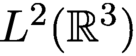 $L^2({\mathbb R}^3)$
that are defined in terms of generalized Laguerre polynomials and spherical harmonics
 $$ \begin{align*} \Lambda_{k,\ell}^m(r,\theta,\varphi) = {\mathrm{e}}^{-r/2} r^\ell L_{k-\ell}^{(2\ell+2)}(r) Y_\ell^m(\theta,\varphi). \end{align*} $$
Here,
 $k\ge 0$
,
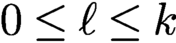 $0\le \ell \le k$
, and
 $-m\le \ell \le m$
. For a recent survey of bases for Sobolev spaces in
 ${\mathbb R}^3$
, we refer the interested reader to Weniger (Reference Weniger2019).
2.7 Evaluation of orthogonal polynomials and Clenshaw’s algorithm
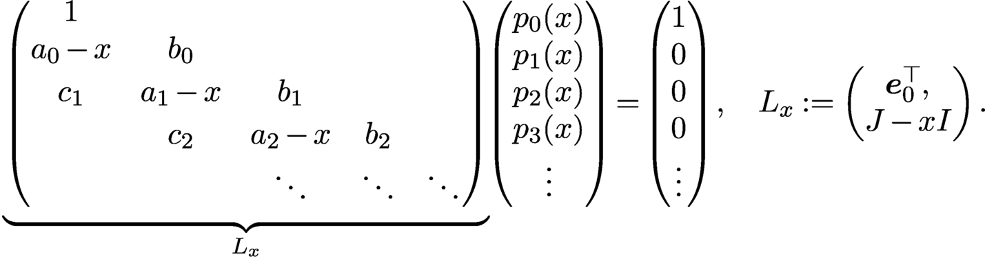
The three-term recurrence relationship for OPs provides an immediate algorithm to evaluate OPs. In the univariate setting, assuming that
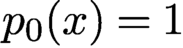 ${p_0(x) = 1}$
, the OPs satisfy the following lower-triangular system (see (2.5)):
 $$ \begin{align} \underbrace{\begin{pmatrix}1 \\ a_0-x & b_0 \\[2pt] c_1 & a_1-x & b_1 \\[2pt] & c_2 & a_2-x & b_2 \\ &&\ddots & \ddots & \ddots\end{pmatrix}}_{L_x}\!\! \begin{pmatrix} p_0(x)\\ p_1(x)\\ p_2(x)\\ p_3(x)\\ \vdots \end{pmatrix} \! = \! \begin{pmatrix} 1\\ 0\\ 0\\ 0\\ \vdots\end{pmatrix}, \quad L_x:= \begin{pmatrix} \boldsymbol{e}_0^{\top},\\ J-xI\end{pmatrix}. \end{align} $$
This is equivalent to
 $\boldsymbol {P}(x)^{\top } = L_x^{-1} \boldsymbol {e}_0$
, where
 $\boldsymbol {e}_0$
is the first unit vector. The linear system in (2.7) can be solved using forward recurrence to evaluate
 $p_0(x),\ldots ,p_{N-1}(x)$
in
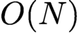 $O(N)$
operations, which we observe to be computationally more efficient in practice than using explicit formulas such as
 $T_n(x) = \cos ( n \cos ^{-1}x)$
for
 $-1\leq x\leq 1$
. One can also use (2.7) to efficiently evaluate functions, that is,
 $$ \begin{align*} f(x) = \boldsymbol{P}(x) \boldsymbol{f} = \boldsymbol{e}_0^{\top} L_x^{-\top} \boldsymbol{f}. \end{align*} $$
This procedure is known as Clenshaw’s algorithm (Clenshaw Reference Clenshaw1955). Therefore, to evaluate
 $f(x)$
one can perform back-substitution using the linear system
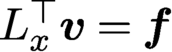 $L_x^{\top } \boldsymbol {v} = \boldsymbol {f}$
and then taking the leading entry. This requires
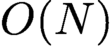 $O(N)$
operations and no extra memory allocations if
 $\boldsymbol {f}$
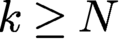
is such that
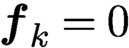 $\boldsymbol {f}_k = 0$
for
 $k\geq N$
.
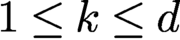
Clenshaw’s algorithm works in multiple dimensions as well, though it is significantly more involved as one needs to work simultaneously with all recurrence relationships, i.e.
 $J_k \boldsymbol {P}(x)^{\top }= \boldsymbol {P}(x)^{\top } \underline x_k$
for
 $1\leq k\leq d$
. In two variables, the analogue of (2.7) is the following block system:
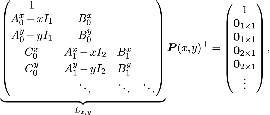 $$ \begin{align} \underbrace{ \begin{pmatrix}1 \\ A_0^x - xI_1 & B_0^x \\[3pt] A_0^y - yI_1 & B_0^y \\[3pt] C_0^x & A_1^x -xI_2 & B_1^x \\[3pt] C_0^y & A_1^y -yI_2 & B_1^y \\ &\ddots & \ddots & \ddots\end{pmatrix}}_{L_{x,y}} \boldsymbol{P}(x,y)^{\top} = \begin{pmatrix}1\\ \mathbf{0}_{1 \times 1}\\ \mathbf{0}_{1 \times 1}\\ \mathbf{0}_{2 \times 1}\\ \mathbf{0}_{2 \times 1}\\ \vdots\end{pmatrix}, \end{align} $$
which is built by interlacing the blocks of
 $$ \begin{align*} {J_x \boldsymbol{P}(x,y)^{\top} = {\boldsymbol{P}(x,y)^{\top} \underline{x}} \quad\text{and}\quad J_y \boldsymbol{P}(y)^{\top} = {\boldsymbol{P}(x)^{\top} \underline{y}}.} \end{align*} $$
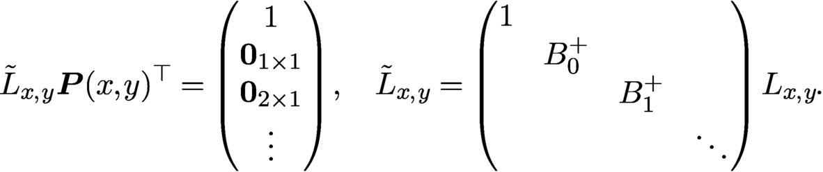
The issue here is that
 $L_{x,y}$
is not a lower-triangular matrix. Fortunately, the blocks given by
 $$ \begin{align*} B_n = \begin{pmatrix}B_n^x\\[2pt] B_n^y\end{pmatrix} \in {\mathbb R}^{(2n+2) \times (n+2)} \end{align*} $$
have full column rank (Dunkl and Xu Reference Dunkl and Xu2014, Theorem 3.3.4) and hence
 $B_n$
has a left-inverse
 $B_n^+$
so that
 $B_n^+ B_n = I_{n+2}$
. Thus we can modify (2.8) to the following lower-triangular linear system:
 $$ \begin{align*} \tilde L_{x,y} \boldsymbol{P}(x,y)^{\top} = \begin{pmatrix} 1\\ \mathbf{0}_{1 \times 1}\\ \mathbf{0}_{2 \times 1}\\ \vdots\end{pmatrix}, \quad \tilde L_{x,y} = \begin{pmatrix}1 \\ & B_0^+ \\ &&B_1^+ \\ &&&\ddots\end{pmatrix} L_{x,y}\!. \end{align*} $$
This can now be solved by forward substitution. A multivariate analogue of Clenshaw’s algorithm follows immediately:
 $$ \begin{align*} f(x,y) = \boldsymbol{P}(x,y) \boldsymbol{f} = \boldsymbol{e}_0^{\top} \tilde L_{x,y}^{-\top} \boldsymbol{f}. \end{align*} $$
The choice of left-inverse
 $B_n^+$
is a delicate issue as it can impact the complexity and stability of multivariable Clenshaw’s algorithm. For the multivariate OPs we often have that
 $B_n$
in (2.8) is a sparse matrix. However, if one naïvely uses the Moore–Penrose pseudo-inverse, then
 $B_n^+$
is typically dense, which leads to a disappointing complexity for evaluating OP expansions. In specific cases, it can be possible to build a sparse
 $B_n^+$
; see Olver, Townsend and Vasil (Reference Olver, Townsend and Vasil2019) for an example on the triangle.
2.8 Recurrences and differential operators
Classical orthogonal polynomials satisfy numerous recurrences – going beyond the three-term recurrence relationship – for differentiation, multiplication and other operations; see Olver et al. (Reference Olver, Lozier, Boisvert and Clark2010, Chapter 18) for a comprehensive summary. The relevant ones for this paper are reviewed in Appendix A and are expressed in the quasimatrix notation.
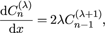
As a brief example, families of classical orthogonal polynomials have the beautiful property that their derivatives are also classical orthogonal polynomials. For example, we have the following formula (Olver et al. Reference Olver, Lozier, Boisvert and Clark2010, 18.9.19):
 $$ \begin{align*} \displaystyle \frac{{\mathrm{d}} C_n^{(\lambda)} }{ {{\mathrm{d}}x} } = 2 \lambda C_{n-1}^{(\lambda+1)}, \end{align*} $$
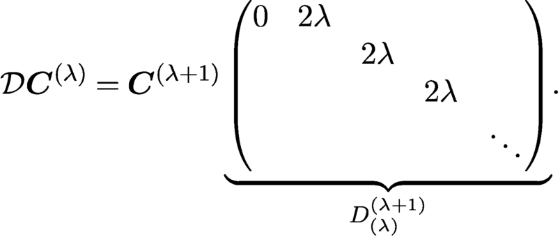
which can be expressed as (see Proposition A.11)
 $$ \begin{align*} {\mathcal D} \boldsymbol{C}^{(\lambda)} = \boldsymbol{C}^{(\lambda+1)} \underbrace{\begin{pmatrix}0 & 2\lambda\\ && 2\lambda \\ &&& 2\lambda \\ &&&& \ddots\end{pmatrix}}_{D_{(\lambda)}^{(\lambda+1)}}\!. \end{align*} $$
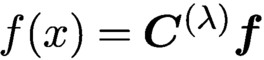
In other words, if
 $f(x) = \boldsymbol {C}^{(\lambda )} \boldsymbol {f}$
, then
 $$ \begin{align*} f'(x) = {\mathcal D} \boldsymbol{C}^{(\lambda)} \boldsymbol{f} = \boldsymbol{C}^{(\lambda+1)} D_{(\lambda)}^{(\lambda+1)} \boldsymbol{f}. \end{align*} $$
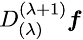
That is, we can efficiently compute the coefficients of the derivative of f in another classical OP expansion via the product
 $D_{(\lambda )}^{(\lambda +1)}\boldsymbol {f}$
.
Another example of an operator is the change from one basis to another (see Proposition A.9):
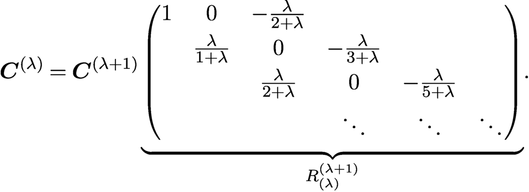 $$ \begin{align*} \boldsymbol{C}^{(\lambda)} = \boldsymbol{C}^{(\lambda+1)} \underbrace{\begin{pmatrix} 1 & 0 & -\frac{\lambda}{2+\lambda} & \\[3pt] & \frac{\lambda}{1+\lambda} & 0 & -\frac{\lambda}{3+\lambda} \\[3pt] & & \frac{\lambda}{2+\lambda} & 0 & -\frac{\lambda}{5+\lambda} \\[3pt] & & & \ddots & \ddots & \ddots \end{pmatrix} }_{R_{(\lambda)}^{(\lambda+1)}}\!. \end{align*} $$
That is, we have
 $$ \begin{align*}f(x) = \boldsymbol{C}^{(\lambda)}(x) \boldsymbol{f} = \boldsymbol{C}^{(\lambda+1)}(x) R_{(\lambda)}^{(\lambda+1)} \boldsymbol{f}. \end{align*} $$
This is a simple example of a transform, which we discuss further in Section4.4. Note that these relationships can be composed to deduce more general operators, for example,
 $$ \begin{align*} f''(x) + x f(x) &= {\mathcal D}^2 \boldsymbol{C}^{(\lambda)}(x) \boldsymbol{f} + x \boldsymbol{C}^{(\lambda)}(x) \boldsymbol{f} \\[12pt] &= {\mathcal D} \boldsymbol{C}^{(\lambda+1)}(x) D_{(\lambda)}^{(\lambda+1)} \boldsymbol{f} + \boldsymbol{C}^{(\lambda)}(x) X_{(\lambda)} \boldsymbol{f} \\[12pt] &= \boldsymbol{C}^{(\lambda+2)} (\underbrace{D_{(\lambda)}^{(\lambda+2)} D_{(\lambda)}^{(\lambda+1)}}_{D_{(\lambda)}^{(\lambda+2)}} + \underbrace{R_{(\lambda+1)}^{(\lambda+2)} R_{(\lambda)}^{(\lambda+1)}}_{R_{(\lambda)}^{(\lambda+2)}} X_{(\lambda)} ) \boldsymbol{f} {,} \end{align*} $$
where
 $X_{(\lambda )}$
is the multiplication-by-x operator for
 $\boldsymbol {C}^{(\lambda )}$
. Such manipulations lead to fast numerical methods for differential equations, as discussed in Section 5.
3 Quadrature
A quadrature rule approximates an integral by a weighted sum of samples of f. The classic interpolatory quadrature rules are Newton–Cotes, Gaussian quadrature and Clenshaw–Curtis, which all take the form
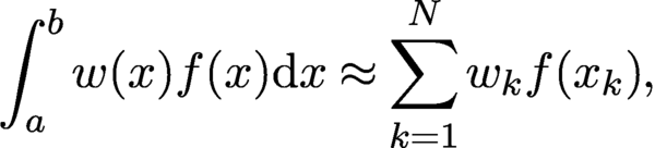 $$ \begin{align} \int_{a}^b w(x) f(x) {{\mathrm{d}}x} \approx \sum_{k=1}^N w_k f(x_k), \end{align} $$
where
 $w(x)$
is a non-negative integrable weight function and
 $\{x_k\}$
and
 $\{w_k\}$
are called the quadrature nodes and weights, respectively. It is known that an N-point Gaussian quadrature exactly integrates polynomials of degree
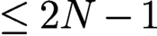 $\leq 2N-1$
. When
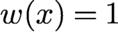 $w(x) = 1$
, the corresponding Gauss quadrature rule is called Gauss–Legendre.
3.1 Weighted Clenshaw–Curtis quadrature
Clenshaw–Curtis quadrature sets the nodes
 $\{x_k\}$
in (3.1) to be Chebyshev points that are trivial to generate. There are at least three main variations on Chebyshev points:
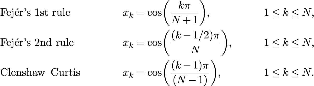 $$ \begin{align*} &\textrm{Fej}\unicode{x00E9}\textrm{r's 1st rule} &\qquad x_k &= \cos\biggl(\dfrac{k\pi}{N+1}\biggr), &\quad &1\leq k\leq N,\\ &\textrm{Fej}\unicode{x00E9}\textrm{r's 2nd rule} & \qquad x_k &= \cos\biggl(\dfrac{(k-1/2)\pi}{N}\biggr), &\quad &1\leq k\leq N,\\ &\text{Clenshaw--Curtis} &\qquad x_k &= \cos\biggl(\dfrac{(k-1)\pi}{(N-1)}\biggr), &\quad &1\leq k\leq N. \end{align*} $$
The differences between these choices for the quadrature nodes are minor, though the Clenshaw–Curtis rule has the advantage that the N-point and
 $2N$
-point nodal sets are nested, allowing for re-use of function evaluation when N is doubled, which can have a significant impact on speed if calculating f is expensive. Therefore Clenshaw–Curtis has become the most popular variant.
The weights
 $\{w_k\}$
are selected so that any polynomial p of degree
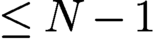 $\leq N-1$
is exactly integrated. That is,
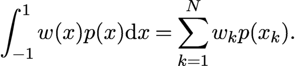 $$ \begin{align*} \int_{-1}^1 w(x) p(x) {{\mathrm{d}}x} = \sum_{k=1}^N w_k p(x_k). \end{align*} $$
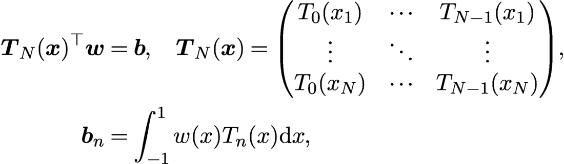
In particular, the quadrature must exactly integrate the Chebyshev polynomials
 $T_0(x),\ldots ,T_{N-1}(x)$
. We find that
 $\{w_k\}$
satisfy the following linear system:
 $$ \begin{align} \boldsymbol{T}_N(\boldsymbol{x})^{\top} \boldsymbol{w} &= \boldsymbol{b}, \quad \boldsymbol{T}_N(\boldsymbol{x}) = \begin{pmatrix}T_0(x_1) & \cdots & T_{N-1}(x_1) \\ \vdots & \ddots & \vdots \\ T_0(x_N) & \cdots & T_{N-1}(x_N)\end{pmatrix}\!, \\ \boldsymbol{b}_n &= \int_{-1}^1 w(x) T_n(x) {{\mathrm{d}}x}, \notag \end{align} $$
where
 $\boldsymbol {x} = (x_1,\ldots ,x_N)^{\top }$
and
 $\boldsymbol {w} = (w_1,\ldots ,w_N)^{\top }$
.
The original papers by Fejér (Reference Fejér1933) and Clenshaw and Curtis (Reference Clenshaw and Curtis1960) were written before the rediscovery of the fast Fourier transform (Cooley and Tukey Reference Cooley and Tukey1965); however, soon afterwards Gentleman (Reference Gentleman1972) noted that the linear system
 $\boldsymbol {T}_N(\boldsymbol {x})^{\top } \boldsymbol {w} = \boldsymbol {b}$
could be solved using the FFT (see Section 4.1). Clenshaw–Curtis quadrature is popular because the rule is accurate, and the nodes and weights can be easily computed in
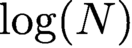
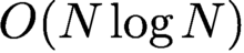 ${O} (N\log N)$
operations. In the 1970s it was one of the only accurate rules for which large quadrature rules could be computed for large N. Today, with fast algorithms to compute many Gauss quadrature rules, we regard Gauss and Clenshaw–Curtis formulas as both valuable for numerical integration (Trefethen Reference Trefethen2008).
Waldvogel (Reference Waldvogel2003) showed a factor of
 $2$
computational saving in computing
 $\{w_k\}$
when
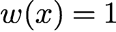 $w(x) = 1$
by exploiting the fact that
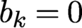 $b_k = 0$
for odd k in (3.2), which allows one to compute the weights using an FFT of half the size. Waldvogel’s speedup can be extended to symmetric weights of the form
 $w(x) = (1-x^2)^\alpha $
for
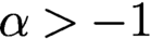 $\alpha>-1$
(Sommariva Reference Sommariva2013).
3.2 The original deviation of Gauss–Legendre quadrature
In contrast to Clenshaw–Curtis quadrature, an N-point Gauss–Legendre quadrature rule exactly integrates polynomials of degree
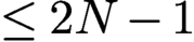 $\leq 2N-1$
by carefully selecting both the nodes and weights. Most textbooks in numerical analysis present the topic in its modern formulation using orthogonal polynomials, as derived by Jacobi (Reference Jacobi1826). However, the original derivation of the Gauss–Legendre quadrature rule by Gauss (Reference Gauss1815) is a beautiful calculation involving continued fractions (Gautschi Reference Gautschi, Butzer and Fehér1981a
).
Let p be any polynomial of degree
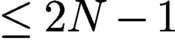 $\leq 2N-1$
and let
 $\Gamma $
be the circle of radius
 $1+\delta $
(for arbitrary small
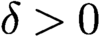 $\delta>0$
) centred at
 $0$
and parametrized in an anticlockwise orientation. Then, from Cauchy’s integral formula we can write
 $$ \begin{align} \int_{-1}^1 p(x) {{\mathrm{d}}x} = \int_{-1}^1 \dfrac{1}{2\pi {\mathrm{i}}}\int_{\Gamma} \dfrac{p(z)}{z-x} {{\mathrm{d}}z} {{\mathrm{d}}x} = \dfrac{1}{2\pi {\mathrm{i}}} \int_{\Gamma} p(z) \phi(z) {{\mathrm{d}}z}, \end{align} $$
where
 $\phi (z) = \log ( (z+1) / (z-1))$
is the analytic function in
 $\mathbb {C}\cup \{\infty \}\setminus [-1,1]$
given by the standard branch of the logarithm, so that
 $\phi $
is positive for
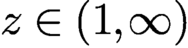 $z\in (1,\infty )$
. Since we want the quadrature rule to be exact, we need
 $$ \begin{align} \int_{-1}^1 p(x) {{\mathrm{d}}x} = \sum_{{k=1}}^N w_kp(x_k) = \dfrac{1}{2\pi {\mathrm{i}}}\int_{\Gamma} p(z) r_N(z) {\mathrm{d}} z, \quad r_N(z) = \sum_{k=1}^N \dfrac{w_k}{z-x_k}, \end{align} $$
where
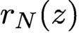 $r_N(z)$
is a
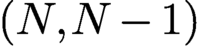 $(N,N-1)$
rational function with poles at the quadrature nodes
 $\{x_k\}$
. By combining (3.3) and (3.4) and noting that p could be any polynomial, we require that
 $$ \begin{align*} \dfrac{1}{2\pi {\mathrm{i}}}\int_{\Gamma} z^j (\phi(z) - r_N(z)) {{\mathrm{d}}z} = 0,\quad 0\leq j\leq 2N-1. \end{align*} $$
Due to the orthogonality of the monomials on the unit circle, we need
 $\phi (z) - r_N(z) = {O} (z^{2N})$
. Gauss would have immediately known how to solve this using continued fractions, which were a popular topic in the early 1800s. In particular,
 $\phi (z)$
can be expressed as the following continued fraction:
 $$ \begin{align*} \phi(z) = \log\biggl( \dfrac{z+1}{z-1} \biggr) = \frac{a_1}{z + \frac{a_2}{z + \frac{a_3}{z + \frac{a_4}{z+\cdots}}}}, \quad a_k = -\frac{k^2}{4k^2-1}. \end{align*} $$
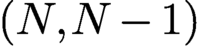
From this expression one can find the N-convergent, which is an
 $(N,N-1)$
rational function
 $r_N(z) = A_{N}(z)/B_{N}(z)$
such that
 $\phi (z) - r_N(z) = {O} (z^{2N})$
. Moreover, it is known that
 $$ \begin{align} B_{k+1}(z) = zB_k(z) - \dfrac{k^2}{4k^2-1}B_{k-1}(z),\quad k\geq 0, \quad B_0(z) = 1, \quad B_{-1}(z) = 0. \end{align} $$
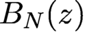
Gauss used this three-term recurrence to derive
 $B_{N}(z)$
and then found its zeros to calculate the quadrature nodes. For example,
 $B_3(z) = z^3-(3/5)z$
, so the three-point Gauss quadrature rule has nodes
 $\{-\sqrt {3/5},0,\sqrt {3/5}\}$
. One can then find the corresponding Gauss–Legendre weights by solving the linear system
 $$ \begin{align*} (\boldsymbol{x}^0 , \boldsymbol{x}^1 , \cdots , \boldsymbol{x}^{N-1})^{\top} \boldsymbol{w} = \boldsymbol{b}, \quad \boldsymbol{b}_k = \int_{-1}^1 x^k {{\mathrm{d}}x} = \dfrac{1-(-1)^{k+1}}{k+1}. \end{align*} $$
For the three-point quadrature, we find that the weights are
 $\{5/9,8/9,5/9\}$
. Today, tables of Gauss–Legendre quadrature nodes and weights can be found throughout the internet and textbooks, though it is more practical to calculate them numerically.
3.3 The Golub–Welsch algorithm
Only a few years after Gauss’s derivation, Jacobi (Reference Jacobi1826) realized the connection between Gauss quadrature and OPs. Jacobi first observed that the recurrence relationship in (3.5) is satisfied by the Legendre polynomials when scaled to be monic. That means that the N-point Gauss–Legendre quadrature nodes satisfy
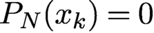 $P_{N}(x_k)=0$
for
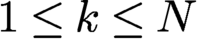 $1\leq k\leq N$
. At the time, Jacobi’s observation did not help one compute Gauss quadrature nodes and weights; however, it did allow Jacobi to generalize Gauss quadrature to other integrable weight functions. In particular, the Gauss quadrature nodes associated to (3.1) are given by the zeros of
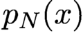 $p_{N}(x)$
, where
 $p_0,p_1,\ldots ,$
is a family of orthogonal polynomials associated to the weight function
 $w(x)$
. In other words, the Gauss quadrature nodes are the zeros of an OP.
The most well-known algorithm for computing Gauss quadrature rules is the Golub–Welsch algorithm (Golub and Welsch Reference Golub and Welsch1969). It is based on the fact that
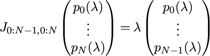 $$ \begin{align*} J_{0:N-1,0:N} \begin{pmatrix}p_0(\lambda)\\ \vdots\\ p_{N}(\lambda)\end{pmatrix} = \lambda \begin{pmatrix}p_0(\lambda)\\ \vdots\\ p_{N-1}(\lambda)\end{pmatrix} \end{align*} $$
and hence, by rearranging, we find
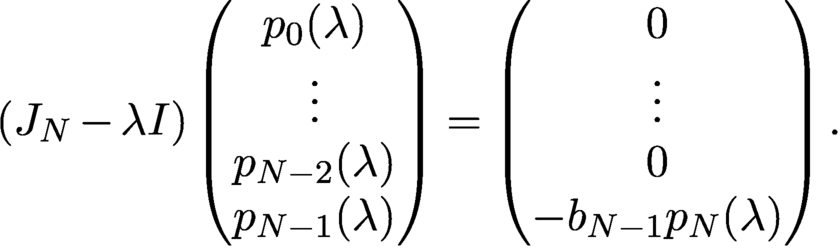 $$ \begin{align} (J_N - \lambda I) \begin{pmatrix}p_0(\lambda)\\ \vdots\\ p_{N-2}(\lambda)\\ p_{N-1}(\lambda)\end{pmatrix} = \begin{pmatrix}0\\ \vdots\\ 0\\ -b_{N-1} p_N(\lambda)\end{pmatrix}. \end{align} $$
Here,
 $J_N$
is the
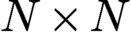 $N\times N$
truncation of the Jacobi operator associated with the OPs. The right-hand side of (3.6) is the zero vector if and only if
 $\lambda $
is a root
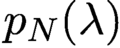 $p_N(\lambda )$
. This means that the quadrature nodes can be computed in
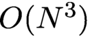 ${O} (N^3)$
operations as an eigenvalue problem involving a tridiagonal matrix. Moreover, if the OPs are orthonormal (which does not change the zeros), then
 $J_{N}$
is a symmetric tridiagonal matrix reducing the cost to only
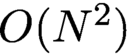 ${O} (N^2)$
operations.
From (3.6), the eigenvector of
 $J_{N}$
corresponding to eigenvalue
 $x_j$
is
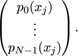 $$ \begin{align*} \begin{pmatrix}p_0(x_j)\\ \vdots\\ p_{N-1}(x_j)\end{pmatrix}. \end{align*} $$
This means that the quadrature weights can be obtained from the eigenvectors of
 $J_{N}$
. Since an N-point Gauss quadrature is exact for polynomials up to degree
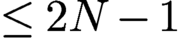 $\leq 2N-1$
, we know that the quadrature weights
 $\boldsymbol {w} = (w_1,\ldots ,w_N)^{\top }$
satisfy
 $$ \begin{align*} \boldsymbol{S}_N(\boldsymbol{x}) D_{\boldsymbol{w}} \boldsymbol{S}_N^{\top}(\boldsymbol{x}) = D_{\boldsymbol{b}}, \quad b_k = \int_{-1}^1 w(x)p_k(x){{\mathrm{d}}x}, \end{align*} $$
where
 $$ \begin{align*} (\boldsymbol{S}_N(\boldsymbol{x}))_{jk} = p_{k-1}(x_j), \quad 1\leq j,\ k\leq N. \end{align*} $$
Therefore
 $D_{\boldsymbol {w}}^{-1} = \boldsymbol {S}_N^{\top }(\boldsymbol {x})\boldsymbol {S}_N(\boldsymbol {x})$
, that is,
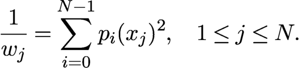 $$ \begin{align*} \dfrac{1}{w_j} = \sum_{i = 0}^{N-1} p_i(x_j)^2, \quad 1\leq j\leq N. \end{align*} $$
In other words, the reciprocal of
 $w_j$
is equal to the sum of the squares of the entries of the eigenvector of
 $J_{N}$
corresponding to eigenvalue
 $x_j$
, where the first entry of the eigenvector is scaled to have the value of
 $1$
.
3.4 Computing Gauss quadrature rules associated with classical orthogonal polynomials
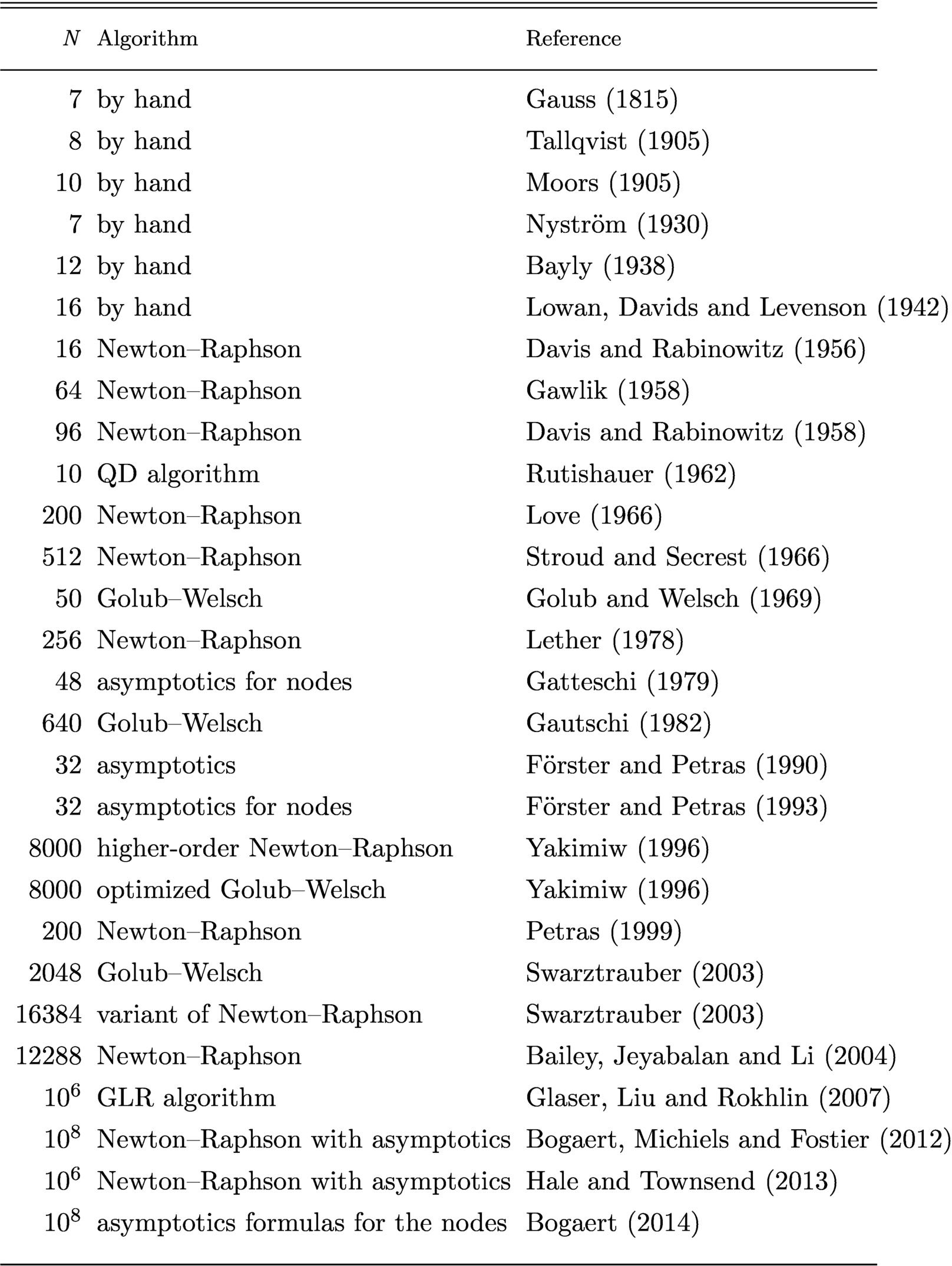
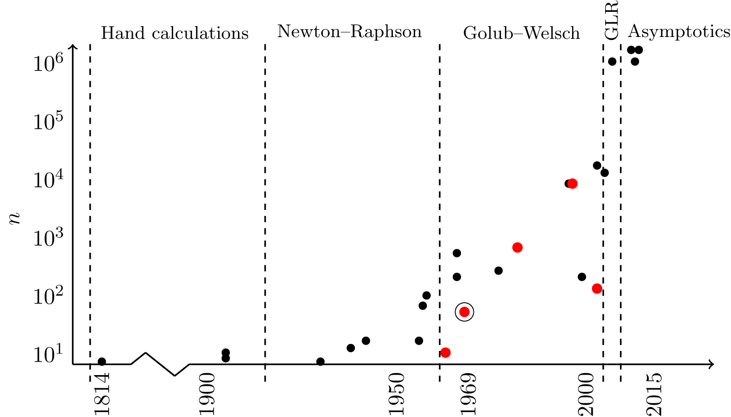
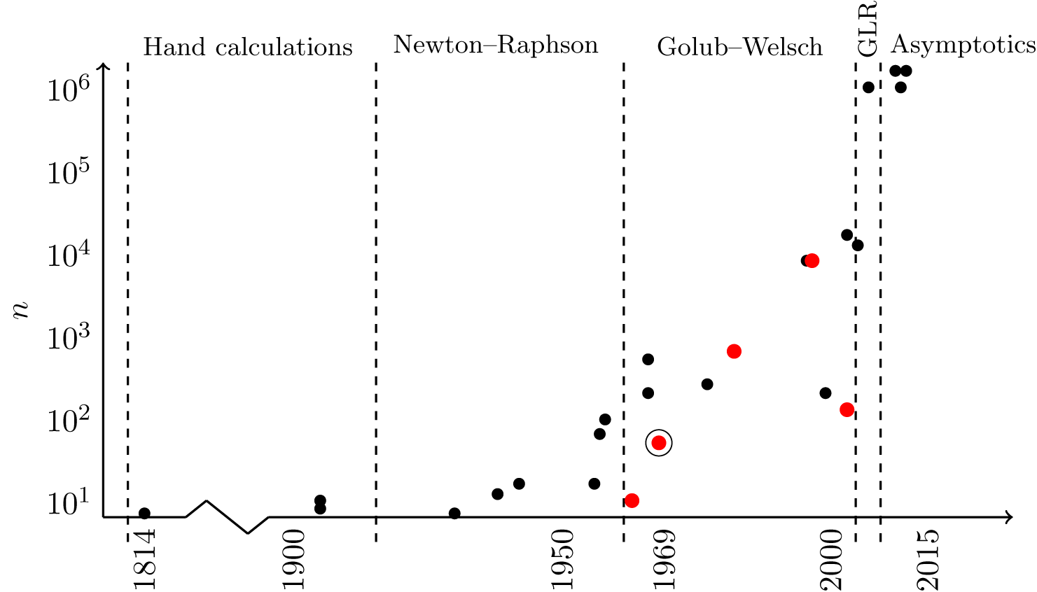
The most important examples of Gauss quadrature rules are those associated with classical OPs. By now, there are hundreds of publications on the subject of computing classical Gauss quadrature rules, and the most efficient algorithms are tailor-made for each quadrature rule. In Table 3.1 we have surveyed the literature on computing Gauss–Legendre quadrature to observe the continuing progression to larger and larger quadrature rules (Townsend Reference Townsend2015). Also, see Figure 3.1. The surprise is that the Golub–Welsch algorithm is not, and never was, the fastest or most accurate algorithm for computing Gauss–Legendre quadrature rules. However, its generality and ease of implementation makes it one of the most widely used algorithms for computing Gauss–Legendre quadrature to this day.
A brief survey of computing Gauss–Legendre quadrature. Originally, small Gauss–Legendre quadrature rules were calculated by brute-force hand calculations; today, a billion quadrature nodes and weights can be computed in a fraction of second on a standard laptop. The value N is the largest reported Gauss–Legendre quadrature rule in the publication.
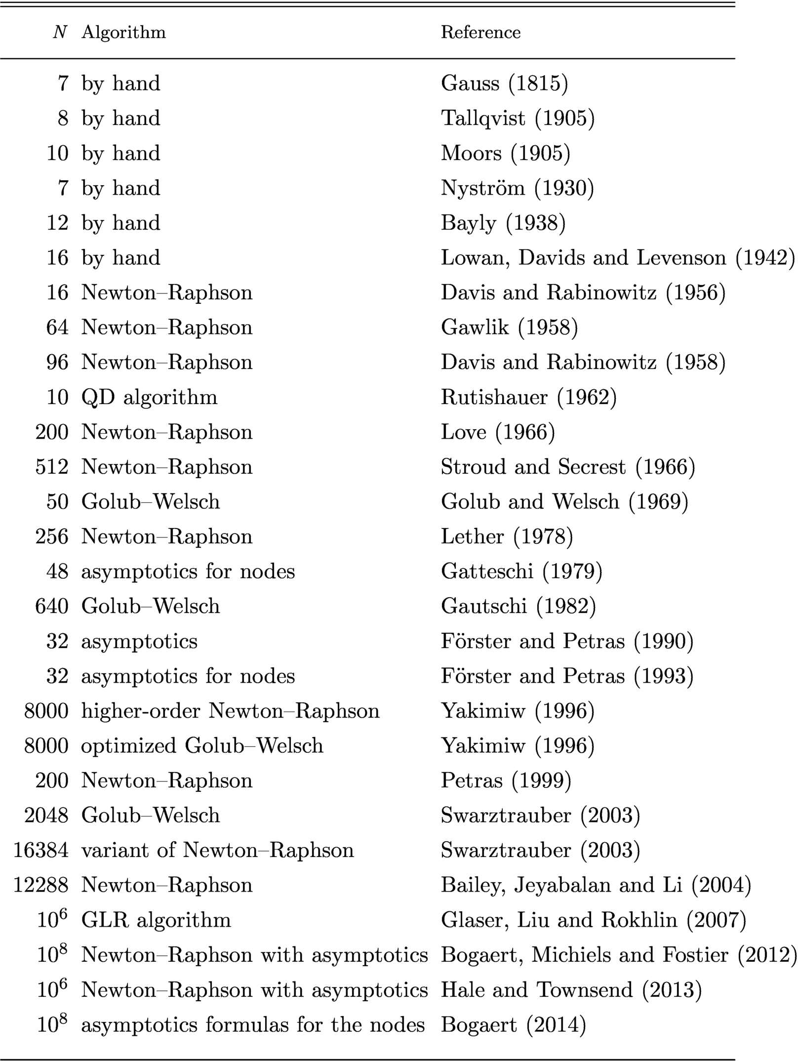
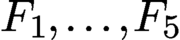
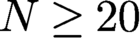
There are now spectacularly fast algorithms for computing Gauss quadrature rules associated with classical OPs. The fastest methods are based on high-order asymptotic formulas for the quadrature nodes (the zeros of the classical OPs) and weights. For example, Bogaert derived asymptotic formulas for the n-point Gauss–Legendre nodes, which are accurate to about 16 digits of precision for any
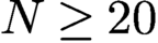 $N\geq 20$
(Bogaert Reference Bogaert2014). Let
 $x_{N,k}=\cos (\theta _{N,k})$
be the kth node in the N-point Gauss quadrature rule. Then
 $$ \begin{align} \theta_{N,k} = \alpha_{N,k} + \sum_{m=1}^5 F_m\biggl(\alpha_{N,k},\dfrac{\cos(\alpha_{N,k})}{\sin(\alpha_{N,k})}\biggr)v_N^{2m} + {O} (v_N^{12}), \quad v_N = \dfrac{1}{N+{1}/{2}}, \end{align} $$
where
 $\alpha _{N,k} = v_Nj_{0,k}$
and
 $j_{0,k}$
is the kth positive zero of the Bessel function
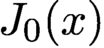 $J_0(x)$
. Here, the functions
 $F_1,\ldots ,F_5$
are known explicitly. For example,
 $$ \begin{align*} F_1(x,u) = \dfrac{1}{8}\dfrac{ux-1}{x}, \quad F_2(x,u) = \dfrac{1}{384}\dfrac{6x^2(1+u^2)+25-u(31u^2+33)x^3}{x^3}, \end{align*} $$
where the remaining formulas for
 $F_3$
,
 $F_4$
and
 $F_5$
along with an asymptotic formula for the quadrature weights can be found in Bogaert (Reference Bogaert2014). For all practical purposes, (3.7) are essentially explicit formulas for the nodes and weights as they can be used for any
 $N\geq 20$
(in double precision) and the cost to evaluate them involves basic arithmetic and trigonometric evaluations. If one wants to compute the nodes to more than 16 digits of precision, then one recommends using
 $\theta _{N,k}$
in (3.7) as an initial guess for Newton’s method on the rootfinding problem
 $P_N(\cos \theta )=0$
(Bogaert et al. Reference Bogaert, Michiels and Fostier2012, Hale and Townsend Reference Hale and Townsend2013).
The history of computing high-order Gauss–Legendre quadrature. A dot represents published work, located at the publication year and the largest Gauss–Legendre rule reported therein. A large red dot is a paper based on variants of the Golub–Welsch algorithm, and the circled red dot is the original paper by Golub and Welsch. GLR represents the Glaser, Liu and Rokhlin (2007) algorithm. Figure reproduced from Townsend (Reference Townsend2015) with permission. Copyright © 2015 Society for Industrial and Applied Mathematics.
Other asymptotic formulas have been derived for Gauss–Jacobi quadrature (Gil, Segura and Temme Reference Gil, Segura and Temme2019b ) as well as Gauss–Laguerre (Gil, Segura and Temme Reference Gil, Segura and Temme2019a ) and Gauss–Hermite (Gil, Segura and Temme Reference Gil, Segura and Temme2018). Again, for high-precision calculations, one can take these asymptotic formulas as initial guesses in Newton’s method (Hale and Townsend Reference Hale and Townsend2013, Townsend, Trogdon and Olver Reference Townsend, Trogdon and Olver2016).
3.5 Computing non-classical Gauss quadrature rules
The previous section shows that having control over the asymptotic behaviour of the zeros of classical OPs can lead to fast iterative-free algorithms for computing Gauss quadrature rules associated with classical weights. Going beyond classical weights, one can build on the recent advances in deriving the asymptotics of general OPs using the Riemann–Hilbert approach (Deift Reference Deift1999) to determine the asymptotic behaviour of the zeros for general weights on the real line. One can alternatively use the numerical solution of the underlying Riemann–Hilbert problem (Olver Reference Olver2012) to calculate numerical asymptotic approximations to OPs and thereby calculate associated Gauss quadrature nodes for relatively general weights (Townsend et al. Reference Townsend, Trogdon and Olver2016).
4 Orthogonal polynomial transforms
Orthogonal polynomial transforms involve computing expansion coefficients in one basis either from function samples or from coefficients in another basis. There are two main types.
-
(1) Synthesis and analysis. The infinite-dimensional synthesis operator is the map that takes OP expansion coefficients to the corresponding function by summing up the expansion. The natural finite-dimensional analogue of the synthesis operator is the map from expansion coefficients to values of the expansion at a specified grid. The infinite-dimensional analysis operator takes a function to its expansion coefficients, and the finite-dimensional counterpart takes function samples to expansion coefficients.
-
(2) Connection problems. It is possible to represent a polynomial in different OP bases. The connection problem is the change-of-basis transform from one OP basis to another.
Our general strategy for synthesis, that is, sampling a polynomial represented in a given OP expansion, is to first represent the polynomial in an OP expansion in which a fast evaluation scheme can be derived based on the FFT. Therefore, we tackle synthesis in two steps: (1) convert one OP basis into another, and (2) evaluate the polynomial in its new OP basis using the FFT. Our strategy for analysis is, therefore, to reverse the process: (1) compute the coefficients in a new OP basis using the FFT, and (2) convert from the new basis into the desired basis.
4.1 Synthesis and analysis based on the fast Fourier transform
The synthesis and analysis transforms that are closely connected to FFTs are the ones related to the four types of Chebyshev expansions and the associated four types of Gauss quadrature nodes (Mason Reference Mason1993). That is, consider the four kinds of Chebyshev nodes,
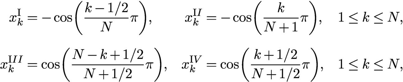 $$ \begin{align} \begin{aligned} x_k^{{\mathrm I}} &= -\cos\biggl(\dfrac{k-{1}/{2}}{N}\pi\biggr), & x_k^{{\mathrm II}} &= -\cos\biggl(\dfrac{k}{N+1}\pi\biggr),& & 1\leq k\leq N, \\[6pt] x_k^{{\mathrm III}} &= \cos\biggl(\dfrac{N-k+{1}/{2}}{N+{1}/{2}}\pi\biggr), & x_k^{{\mathrm IV}} &= \cos\biggl(\dfrac{k+{1}/{2}}{N+{1}/{2}}\pi\biggr),& & 1\leq k\leq N, \end{aligned}\end{align} $$
which are the zeros of
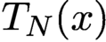 $T_N(x)$
,
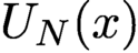 $U_N(x)$
,
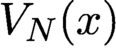 $V_N(x)$
and
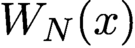 $W_N(x)$
, respectively. There are 16 types of Chebyshev transforms, corresponding to the four choices of nodes in (4.1) and the four choices of Chebyshev polynomials (Püschel and Moura Reference Püschel and Moura2003).
For example, if
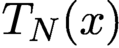 $T_N(x)$
is selected and we are given coefficients
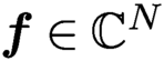 $\boldsymbol {f} \in {\mathbb C}^N$
so that
 $$ \begin{align*} f(x) = {\boldsymbol{T}}_N(x) \boldsymbol{f} {,} \end{align*} $$
where
 $\boldsymbol {T}_N = (T_0,\ldots ,T_{N-1})$
, then the four synthesis transforms are
 $$ \begin{align*} \boldsymbol{T}_N(\boldsymbol{x}^{{\mathrm I}}) \boldsymbol{f}, \quad \boldsymbol{T}_N(\boldsymbol{x}^{\mathrm{II}}) \boldsymbol{f}, \quad\boldsymbol{T}_N(\boldsymbol{x}^{\mathrm{III}}) \boldsymbol{f}, \quad\boldsymbol{T}_N(\boldsymbol{x}^{\mathrm{IV}}) \boldsymbol{f}, \end{align*} $$
or, equivalently,
 $$ \begin{align*} \sum_{n=0}^{N-1} f_n T_n( x_k^{\mathrm{I}} ), \quad \sum_{n=0}^{N-1} f_n T_n( x_k^{\mathrm{II}} ), \quad \sum_{n=0}^{N-1} f_n T_n( x_k^{\mathrm{III}} ), \quad {\sum_{n=0}^{N-1} f_n T_n( x_k^{\mathrm{IV}} )}. \end{align*} $$
Since
 $T_n(x) = \cos ( n \cos ^{-1}x)$
for
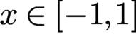 $x\in [-1,1]$
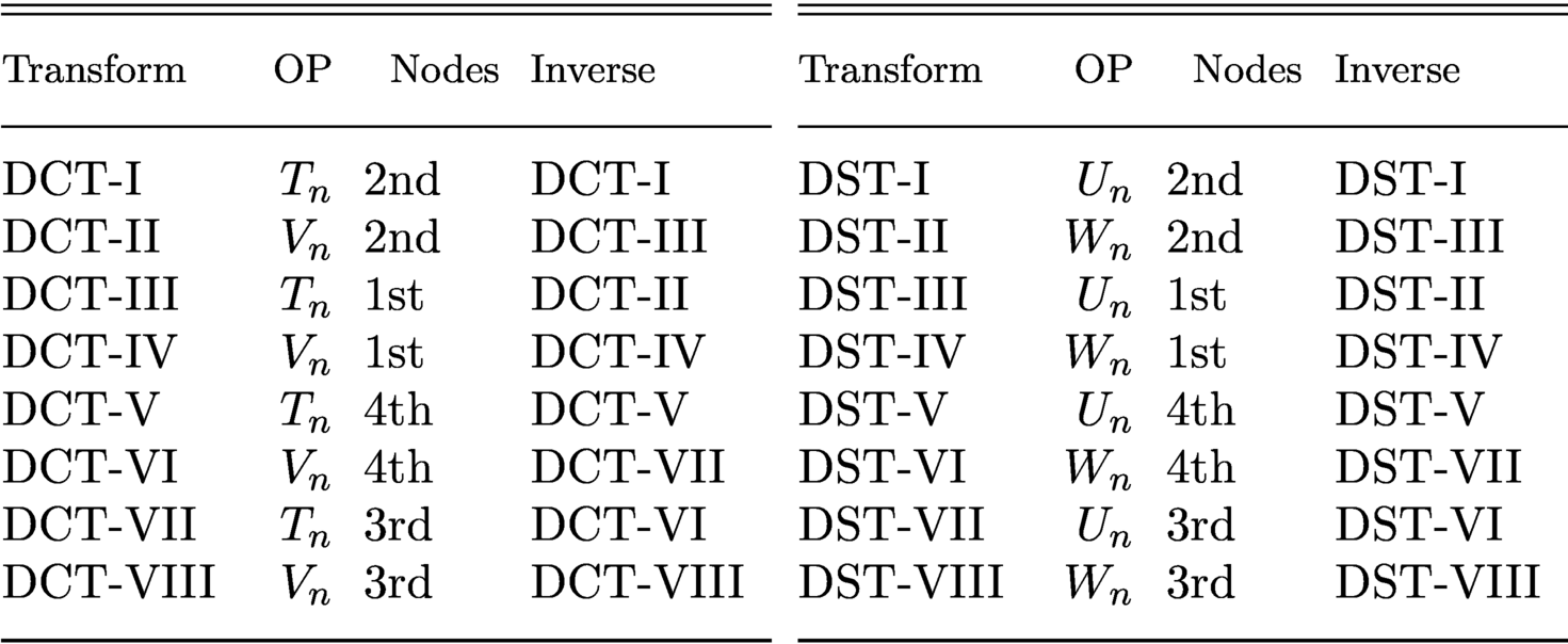
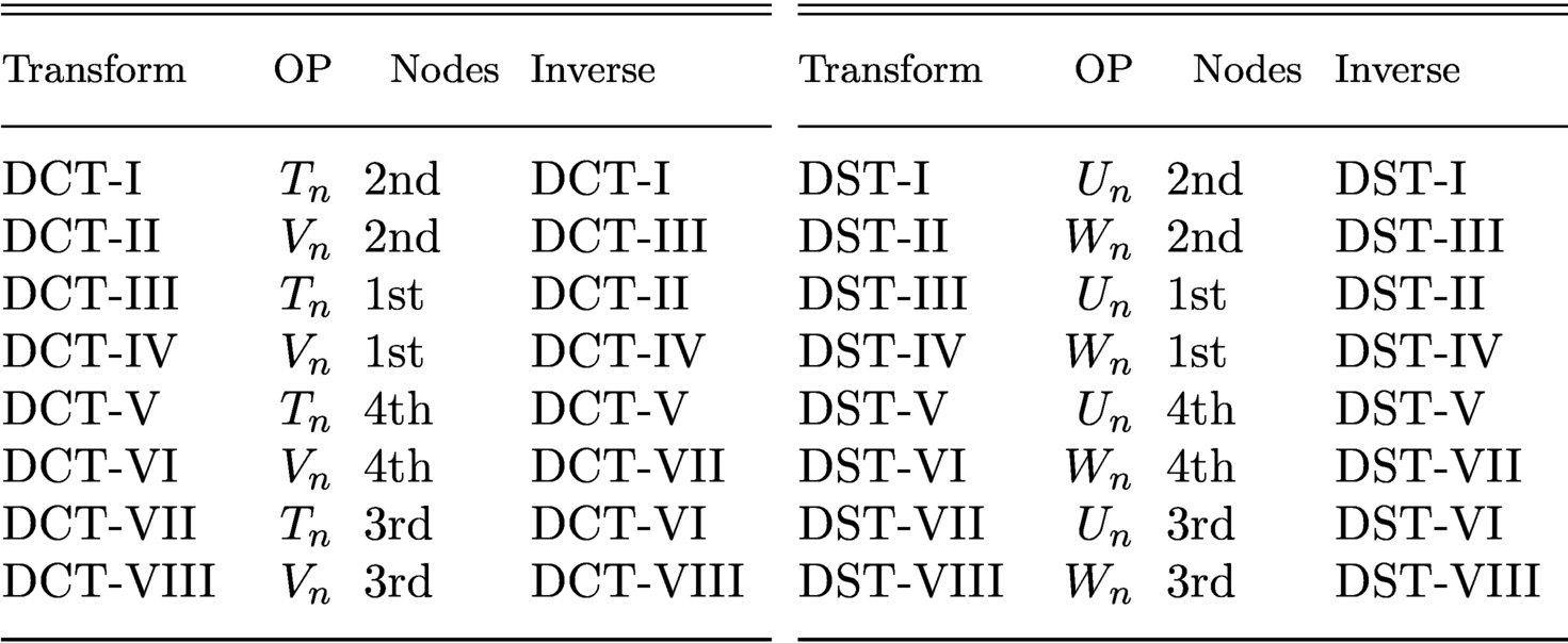
, these transformations can all be related to discrete cosine transforms (DCTs), which can be computed using an FFT. Table 4.1 enumerates all the different discrete sine and cosine transforms and their relations with the four kinds of Chebyshev polynomials and their respective Gauss–Chebyshev nodes. More precise details on the connections can be found in Püschel and Moura (Reference Püschel and Moura2003). When combined with non-uniform fast Fourier transforms (Dutt and Rokhlin Reference Dutt and Rokhlin1993, Potts and Steidl Reference Potts and Steidl2003, Greengard and Lee Reference Greengard and Lee2004, Ruiz-Antolín and Townsend Reference Ruiz-Antolín and Townsend2018), fast algorithms for synthesis and analysis at sample locations that deviate from Gauss–Chebyshev points are also possible.
Connection between the discrete cosine and sine transforms of various types and the evaluation of the four types of Chebyshev series at the four kinds of Chebyshev nodes. Equivalence of these transforms holds up to a diagonal scaling.
More generally, given the three-term recurrence relationships for OPs, there are fast algorithms for synthesis and analysis at the associated Gauss quadrature nodes (Tygert Reference Tygert2010b ). However, the direct connection to FFTs is no longer present. Instead, our general strategy is to convert (using the connection problem) into one of the Chebyshev bases. The fast algorithms in Tygert (Reference Tygert2010b ) are only possible when the recurrence relationships for the OPs are either known explicitly or fast to compute. For several multivariate orthogonal polynomials and semiclassical orthogonal polynomials, the recurrence relationships can be costly to compute (Snowball and Olver Reference Snowball and Olver2020).
4.2 The connection problem
The connection problem concerns the question of how to change between different basis expansions, and in particular how to do so fast. We can state this in terms of connection coefficients.
Definition 4.1. Let
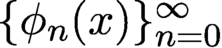 $\{\phi _n(x)\}_{n=0}^\infty $
be a family of orthogonal functions with respect to a measure
 $\mu $
and let
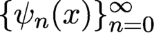 $\{\psi _n(x)\}_{n=0}^\infty $
be another family of orthogonal functions with respect to a measure
 $\hat \mu $
. Assuming that
 $\{\psi _n(x)\}_{n=0}^\infty \subset L^2[\hat \mu ]$
, we have
 $$ \begin{align} \phi_n(x) = \sum_{\ell=0}^\infty c_{\ell,n} \psi_\ell(x), \quad c_{\ell,n} = \dfrac{\langle \psi_\ell, \phi_n\rangle_{{\mathrm d}\mu}}{\langle \psi_\ell, \psi_\ell\rangle_{{\mathrm d}\mu}}, \end{align} $$
where
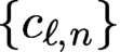 $\{c_{\ell ,n}\}$
are referred to as the connection coefficients.
In quasimatrix notation, (4.2) can be conveniently expressed as
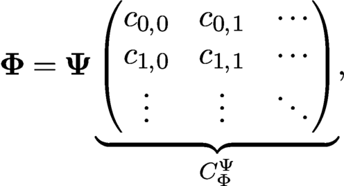 $$ \begin{align*} \boldsymbol{\Phi} = \boldsymbol{\Psi}\underbrace{ \begin{pmatrix}c_{0,0} & c_{0,1} & \cdots\\ c_{1,0} & c_{1,1} & \cdots \\ \vdots & \vdots & \ddots\end{pmatrix}}_{C_\Phi^\Psi}\!, \end{align*} $$
where
 $\boldsymbol {\Phi } := (\phi _0 \mid \phi _1 \mid \cdots )$
and
 $\boldsymbol {\Psi } := ( \psi _0 \mid \psi _1 \mid \cdots )$
. This means that connection coefficients are the entries of a basis conversion matrix. In particular, given a polynomial expansion
 $u(x) = \boldsymbol {\Phi }(x) \boldsymbol {u}$
, we have that
 $u(x) = \boldsymbol {\Psi }(x)C_\Phi ^\Psi \boldsymbol {u} = \boldsymbol {\Psi }(x) \boldsymbol {v}$
, where
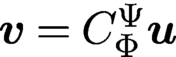 $\boldsymbol {v} = C_\Phi ^\Psi \boldsymbol {u}$
are the expansion coefficients in
 $\boldsymbol {\Psi }$
.
We call connection problems where
 $\boldsymbol {\Phi }$
and
 $\boldsymbol {\Psi }$
are orthogonal with respect to the same measure measure-preserving. If
 $\boldsymbol {\Phi }$
and
 $\boldsymbol {\Psi }$
are orthogonal with respect to different measures, then we call the connection problem measure-perturbing. There is an interesting connection between measure-perturbing connection problems and sparse recurrence relationships (Narayan and Hesthaven Reference Narayan and Hesthaven2012). In the measure-perturbing case, we wish to apply
 $N\times N$
truncations of
 $C_\Phi ^\Psi $
to vectors in
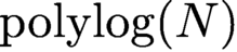
 $O({N{\mathrm polylog}(N))})$
operations.Footnote
3
As we shall see later, the measure-preserving case requires the application of rectangular truncations of
 $C_\Phi ^\Psi $
, though both dimensions are still asymptotically governed by N.
In the special case of connection problems between two complete degree-graded orthogonal polynomial bases, the connection coefficient matrix is upper-triangular. To emphasize this we use the notation
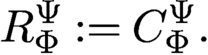 $$ \begin{align*} R_\Phi^\Psi := C_\Phi^\Psi. \end{align*} $$
If
 $\boldsymbol {\Phi }$
and
 $\boldsymbol {\Psi }$
are orthonormal with respect to the same measure, we use the notation
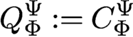 $$ \begin{align*} Q_\Phi^\Psi := C_\Phi^\Psi \end{align*} $$
to emphasize that it is a matrix with orthonormal columns. Moreover, if
 $\deg (\phi _k) = \deg (\psi _k)$
for
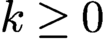 $k\geq 0$
, then
 $Q_\Phi ^\Psi $
is a diagonal matrix with
 $\pm 1$
on the diagonal due to the uniqueness of univariate OPs. Therefore, we focus on the cases (1)
 $\deg (\phi _n) = \deg (\psi _n) + 1$
, (2)
 $\deg (\phi _n) = \deg (\psi _n) + 2$
with a certain symmetry in the domain and weight function, and (3)
 $\deg (\phi _n) \gg \deg (\psi _n)$
.
Univariate OP transforms are an essential building block in the multivariate setting. For tensor product multivariable OPs (see Section 2.6.1), the transforms are Kronecker products of univariate transforms. For OPs from non-degenerate versions of Koornwinder’s construction (see Section 2.6.2), both the measure-preserving and measure-perturbing transforms are required. We illustrate this via spherical harmonics, due to their prevalence in applications.
4.3 Chebyshev polynomials
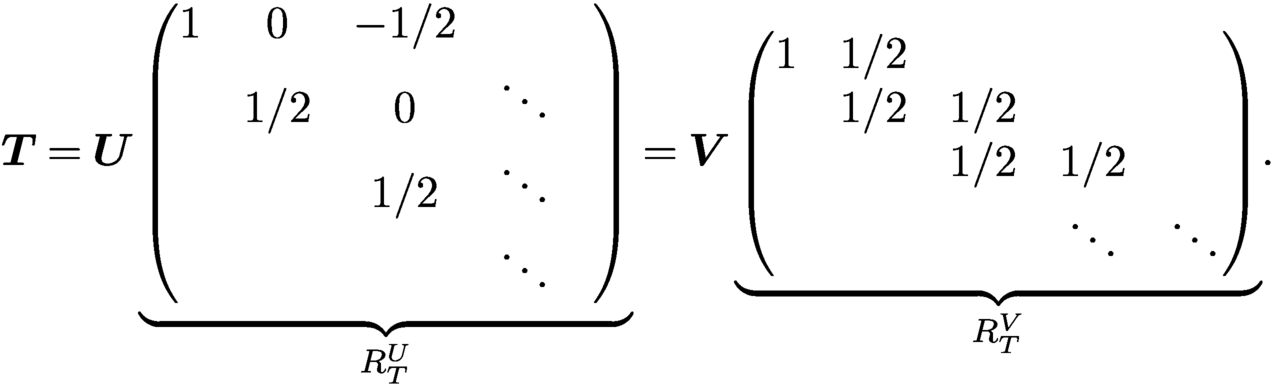
There are sparse relationships between the four types of Chebyshev polynomials, coming from trigonometric identities, which lead to sparse connection problems. For example, we have (Proposition A.13)
 $$ \begin{align*} \boldsymbol{T} = \boldsymbol{U} \underbrace{ \begin{pmatrix} 1 & 0 & -1/2 \\ & 1/2 & 0 & \ddots \\ && 1/2 & \ddots & \\ &&&\ddots &\end{pmatrix}}_{R_T^U} = \boldsymbol{V} \underbrace{ \begin{pmatrix} 1 & 1/2 \\ & 1/2 & 1/2 \\ && 1/2 & 1/2 \\ &&&\ddots & \ddots \end{pmatrix}}_{R_T^V}\!. \end{align*} $$
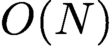
For a polynomial of degree
 $\leq N$
, one can efficiently convert between Chebyshev bases in
 $O(N)$
operations by multiplying or inverting via back-substitution with these connection coefficient matrices. This is useful if one already has access to Chebyshev coefficients of a particular type, especially if the coefficients are known to a good relative accuracy, which is preserved under these conversions provided they decay reasonably quickly, or as an alternative to implementing all 16 types of DCTs and DSTs.
4.4 Ultraspherical polynomials
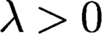
For any
 $\lambda> 0$
, we have (Proposition A.9)
 $$ \begin{align*} \boldsymbol{C}^{(\lambda)} \begin{pmatrix}\lambda \\ & \lambda + 1\\ & & \lambda + 2 \\ & && \ddots \end{pmatrix} = \boldsymbol{C}^{(\lambda+1)}\begin{pmatrix} \lambda & 0 & -\lambda \\ & \lambda & 0 & -\lambda\\ && \ddots & \ddots & \ddots \end{pmatrix}\!, \end{align*} $$
which can also be written as
 $$ \begin{align*} {\boldsymbol{C}^{(\lambda)} = \boldsymbol{C}^{(\lambda+1)} R_{(\lambda)}^{(\lambda+1)}.} \end{align*} $$
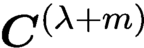
For a polynomial of degree
 $\leq N$
, one can convert between
 $\boldsymbol {C}^{(\lambda )}$
and
 $\boldsymbol {C}^{(\lambda +m)}$
bases, where m is an integer, by applying or inverting m banded operators in
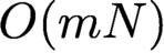 $O(m N)$
operations. Moreover, one can also efficiently convert between Jacobi bases
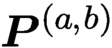 $\boldsymbol {P}^{(a,b)}$
and
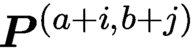 $\boldsymbol {P}^{(a+i,b+j)}$
, where i and j are integers, using the bidiagonal conversion operators in Proposition A.3.
4.5 The Chebyshev–Legendre transform and its inverse
Many different algorithms accelerate the Chebyshev–Legendre transform and its inverse, that is, applying the conversions
 $R_T^P$
and
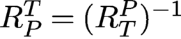 $R_P^T = (R_T^P)^{-1}$
, where
 $$ \begin{align*} \boldsymbol{T} = \boldsymbol{P} R_T^P, \quad \boldsymbol{P} = \boldsymbol{T} R_P^T. \end{align*} $$
These include an adaptation of the fast multipole method (Alpert and Rokhlin Reference Alpert and Rokhlin1991), algorithms based on semi-separable matrices (Keiner Reference Keiner2008, Keiner Reference Keiner2009, Keiner Reference Keiner2011) and analysis of the Toeplitz–Hankel structure of the connection coefficients (Townsend, Webb and Olver Reference Townsend, Webb and Olver2018). There are also methods for direct synthesis and analysis using the asymptotics of Legendre polynomials (Orszag Reference Orszag1986, Mori, Suda and Sugihara Reference Mori, Suda and Sugihara1999, Hale and Townsend Reference Hale and Townsend2014, Slevinsky Reference Slevinsky2018b ) as well as ideas related to non-oscillatory phase functions (Bremer and Yang Reference Bremer and Yang2019).
The Chebyshev–Legendre transform has the beneficial feature that the conversion matrices are known explicitly, albeit they are not banded.
Lemma 4.2 (Alpert and Rokhlin Reference Alpert and Rokhlin1991).
The connection operators for Chebyshev–Legendre are given by
 $$ \begin{align*} \pi R_P^T & = \begin{pmatrix}\Lambda(0)^2 & 0 & \Lambda(1)^2 & 0 & \Lambda(2)^2 & \cdots \\ & 2\Lambda(0) \Lambda(1) & 0 & 2 \Lambda(1) \Lambda(2) &0 & \ddots \\ && 2\Lambda(0) \Lambda(2) & 0 & 2 \Lambda(1) \Lambda(3) & \ddots \\ &&& \ddots & \ddots & \ddots \end{pmatrix}\!, \\[15pt] R_T^P &= \begin{pmatrix}1 & 0 & \! -\dfrac{\Lambda(0) \Lambda(1/2)}{6} \! & 0 & \! -\dfrac{\Lambda(1)\Lambda(3/2)}{10} \! & \cdots \\ & \displaystyle \frac{\sqrt \pi }{ 2 \Lambda(1)} & 0 & \! -\dfrac{9\Lambda(0)\Lambda(3/2)}{20} \! & 0 & \cdots \\ && \displaystyle \frac{\sqrt \pi }{ 2 \Lambda(2)} & 0 & \! -\dfrac{5 \Lambda(0)\Lambda(3/2)}{7}\! \\ &&& \ddots & \ddots & \ddots \end{pmatrix}\! , \end{align*} $$
where
 $\Lambda (k) = \Gamma (k+1/2) /\Gamma (k+1)$
. More explicitly, for
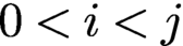 $0 < i < j$
and
 $i+j$
even, we have
 $(R_P^T)_{ij} = {\mathcal M}(i,j)$
and
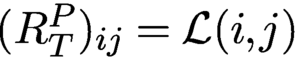 $(R_T^P)_{ij} = {\mathcal L}(i,j)$
, where
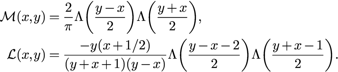 $$ \begin{align*} {\mathcal M}(x,y) &= \displaystyle \frac{2 }{ \pi} \Lambda\biggl(\displaystyle \frac{y-x }{ 2}\biggr) \Lambda\biggl(\displaystyle \frac{y+x }{ 2}\biggr), \\ {\mathcal L}(x,y) &= \displaystyle \frac{-y (x+1/2) }{ (y+x+1)(y-x)} \Lambda\biggl(\displaystyle \frac{y-x -2 }{ 2}\biggr) \Lambda\biggl(\displaystyle \frac{y+x-1 }{ 2}\biggr). \end{align*} $$
Proof. There are a number of ways to prove this, but we introduce a non-standard way based on expressing
 $R_P^T$
as the solution to a Sylvester equation of the form
 $$ \begin{align} A V = B V \Lambda {,} \end{align} $$
where A and B are upper-triangular banded matrices and
 $\Lambda $
is diagonal. This version of the proof will lead to generalization of the construction in a way that can be exploited for other families of OPs via the algorithm in Section 4.6.4. As the columns of V are discrete eigenvectors, the solution is unique up to diagonal column scaling. Thus, if we specify the diagonal entries of V, then we can recover the remaining entries by back-substitution.
The differential equation satisfied by the Legendre quasimatrix,
 $\boldsymbol {P}$
, is
 $$ \begin{align*} [(x^2-1) {\mathcal D}^2 + 2x {\mathcal D}] \boldsymbol{P} = \boldsymbol{P} \Lambda, \end{align*} $$
where
 $\Lambda $
is a diagonal matrix satisfying
 $\Lambda _{n,n} = n (n+1)$
. Substituting in
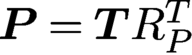 $\boldsymbol {P} = \boldsymbol {T} R_P^T$
, we find that the Sylvester equation is
 $$ \begin{align*} {AR_P^T = BR_P^T\Lambda.} \end{align*} $$
Here, we used the relationship
 $$ \begin{align*} [(x^2-1) {\mathcal D}^2 + 2x {\mathcal D}] \boldsymbol{T} = \boldsymbol{U} \underbrace{\bigl[-L_{(2)}^U D_T^{(2)} + 2X_U D_T^U\bigr]}_A, \quad \boldsymbol{T} = \boldsymbol{U} \underbrace{R_T^U}_B, \end{align*} $$
where
 $D_T^U$
is given in Proposition A.15,
 $D_T^{(2)}$
is given in Proposition A.11,
 $L_{(2)}^U$
is given in Proposition A.10, and
 $X_U$
is the multiplication-by-x operator for
 $\boldsymbol {U}$
. Direct inspection shows that the proposed formula for
 $R_P^T$
satisfies this (banded) Sylvester equation, and it is the unique solution due to the normalizations of the polynomial families. □
The existing methods for computing the Chebyshev–Legendre transform build on having an explicit formula for the entries. Here we outline various approaches.
4.5.1 The low-rank approximation approach
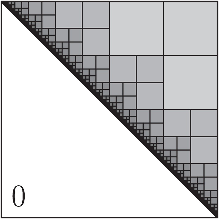
Alpert and Rokhlin (Reference Alpert and Rokhlin1991) exploit the fact that the entries of
 $R_T^P$
and
 $R_P^T$
can be written in terms of the bivariate smooth functions
 ${\mathcal M}$
and
 ${\mathcal L}$
. Then the conversion matrices are hierarchically subdivided using bivariate Chebyshev approximations of
 ${\mathcal M}$
and
 ${\mathcal L}$
.
Definition 4.3 (Keiner Reference Keiner2009).
A square
 $[x_0,x_0+c]\times [y_0,y_0+c]\subset \mathbb {R}^2$
with
 $c>0$
is said to be well-separated if
 $y_0-x_0\ge 2c$
.
Alpert and Rokhlin (Reference Alpert and Rokhlin1991) prove rigorous error bounds for bivariate Chebyshev approximations to
 ${\mathcal M}$
and
 ${\mathcal L}$
on well-separated squares. The error bounds are derived by keeping one of the variables of
 ${\mathcal M}$
and
 ${\mathcal L}$
fixed and letting the other variable freely range over the possible values it may take in S. For example, keeping y fixed, error bounds are derived for Chebyshev interpolants to
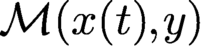 ${\mathcal M}(x(t), y)$
on well-separated squares, where
 $$ \begin{align*} x(t) = x_0+c(t+1)/2,\quad t\in[-1,1]. \end{align*} $$
Theorem 4.4 (Keiner Reference Keiner2009).
Let
 ${\mathcal M}_k$
denote the Chebyshev interpolant at k points to
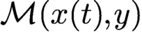 ${\mathcal M}(x(t),y)$
. Then, for
 $c> 1$
, we have
 $$ \begin{align*} \mathop{\mathrm{sup}}_{t\in[-1,1]}{|{\mathcal M}(x(t),y)-{\mathcal M}_k(x(t),y)|} \le \dfrac{4M\rho^{-k}}{\rho-1}, \end{align*} $$
where
 $M = (2\sqrt {2}\exp (5/3))/\pi $
and
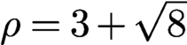 $\rho = 3+\sqrt {8}$
.
Thus a Chebyshev polynomial interpolant of degree at most
 $$ \begin{align*} \biggl\lceil\log \biggl(\dfrac{4\sqrt{2}\,{\mathrm{e}}^{{5}/{3}}}{\pi(1+\sqrt{2})\varepsilon}\biggr)\bigg/\log(3+\sqrt{8})\biggr\rceil \end{align*} $$
is sufficient to approximate
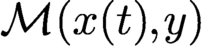 ${\mathcal M}(x(t),y)$
to within
 $\varepsilon>0$
on any well-separated square. This naturally leads to a hierarchical partitioning of the connection coefficient matrix, as depicted in Figure 4.1. The matrix
 ${\mathcal L}$
has a similar structure.
An illustration of the hierarchical decomposition of the Chebyshev–Legendre connection coefficients. The opacity illustrates the data-sparsity in the hierarchical decomposition.
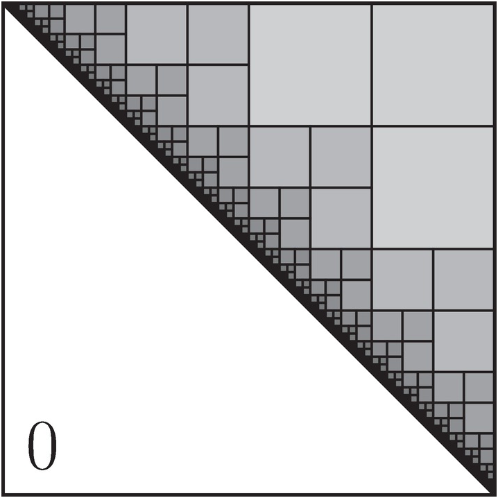
This approximation to
 ${\mathcal M}$
can be applied to a vector in
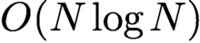 $O(N \log N)$
operations. If the function
 ${\mathcal M}$
is interpolated in both variables, and just the right information is translated up and down the hierarchy, then the fast multipole method (FMM) (Greengard and Rokhlin Reference Greengard and Rokhlin1987, Martinsson and Rokhlin Reference Martinsson and Rokhlin2007) accelerates the same matrix–vector product in
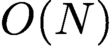 $O(N)$
operations. This approach has a relatively large pre-computation cost, where by pre-computation we mean any computation that can be completed before knowing the vector. Still, once the data structure is created, it is the fastest approach for computing the Chebyshev–Legendre transform, making it ideal for applications in which the repeated action of a Chebyshev–Legendre transform is required.
4.5.2 The Toeplitz–Hankel approach
The method of Townsend et al. (Reference Townsend, Webb and Olver2018) takes an alternative approach with a lower pre-computational cost. Observe that
 $R_T^P$
can be expressed as the upper-triangular component of a diagonally scaled Hadamard (entry-wise) product of a Toeplitz matrix and a Hankel matrix. That is,
 $$ \begin{align*} R_P^T = D [T \circ H], \end{align*} $$
where
 $D = \operatorname {diag}{({1}/{\pi }, {2}/{\pi }, {2}/{\pi }, \ldots )}$
,
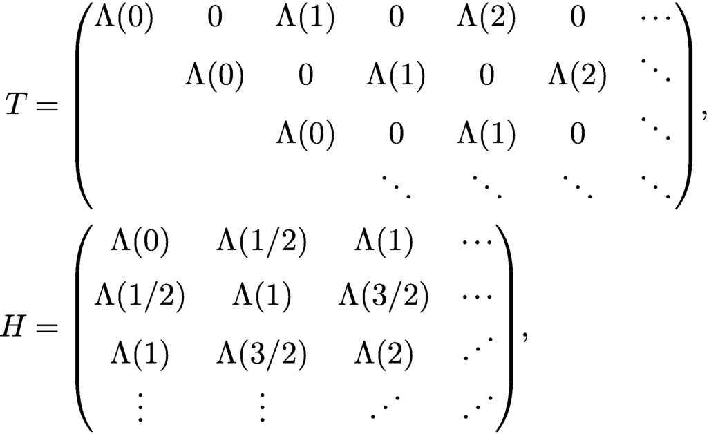
and ‘
 $\kern.25pt\circ $
’ denotes the Hadamard product, i.e.
 $(A \circ B)_{kj} = A_{kj} B_{kj}$
. Now, Townsend et al. (Reference Townsend, Webb and Olver2018) prove that H is a positive definite matrix and can be well-approximated by a low-rank matrix. In particular, it can be well-approximated as
 $H \approx \sum _{s=1}^r a_s \ell _s \ell _s^{\top }$
, where
 $r = {O} (\log N)$
, using a pivoted Cholesky algorithm. It then follows that
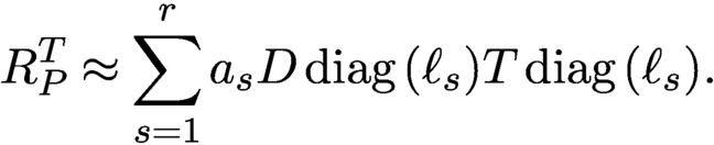 $$ \begin{align*} R_P^T \approx \sum_{s=1}^r a_s D \operatorname{diag}{(\ell_s)} T \operatorname{diag}{(\ell_s)}. \end{align*} $$
Since applying an
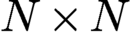 $N\times N$
Toeplitz matrix to a vector costs
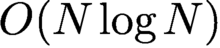 $O(N \log N)$
operations, we can compute
 $R_P^Tv$
in
 $O(r N \log N) = O(N \log ^2 N) $
operations. This extends naturally to applying
 $R_T^P$
and some Jacobi–Jacobi transforms, where the explicit representation is also known.
4.6 The measure-perturbing connection problem
The algorithms mentioned above for Chebyshev–Legendre transforms are based on the explicit formula for the connection coefficients as the ratio of gamma functions. Beyond classical orthogonal polynomials, we cannot expect to have such precise information on the connection coefficients.Footnote 4 Here we generalize the above construction based on the following observation: it suffices to know that the conversion matrix satisfies a triangular banded Sylvester equation (4.3) to apply it fast using a divide-and-conquer algorithm. The approach is formally equivalent to Keiner’s divide-and-conquer algorithms for eigenvectors of semi-separable matrices but expresses the problems in the more natural format of triangular-banded generalized eigenvalue problems (GEPs). The GEP form can be deduced via recurrence relationships and differential equations in an analogous way to the proof of Lemma 4.2.
Many classes of orthogonal polynomials satisfy a linear homogeneous differential equation. For example, classical orthogonal polynomials are the polynomial eigenfunctions of the second-order differential operators of the form
 $$ \begin{align} \sigma p_n^{\prime\prime} + \tau p_n' = \lambda_n p_n, \end{align} $$
where
 $\sigma $
is a polynomial of degree at most two,
 $\tau $
is a polynomial of degree one, and
 $\lambda _n = ({n}/{2}) [(n-1)\sigma ^{\prime \prime } + 2\tau ']$
. This can be extended beyond classical orthogonal polynomials; see Appendix C. Upon closer inspection, both sides of (4.4) are degree-preserving. Since
 $\sigma $
and
 $\tau $
are also polynomial, it follows that identities for differentiation of classical orthogonal polynomials allow one to obtain an upper-triangular and banded discretization of the differential equation. We now demonstrate this for connection problems involving Jacobi, Laguerre and ultraspherical polynomials.
4.6.1 The Jacobi–Jacobi connection problem
The Jacobi–Jacobi connection problem relates two families of Jacobi polynomials. We have
 $$ \begin{align*} \boldsymbol{P}^{(\alpha,\beta)} = \boldsymbol{P}^{(\gamma,\delta)} R_{(\alpha,\beta)}^{(\gamma,\delta)} \end{align*} $$
for some
 $\alpha , \beta , \gamma , \delta>-1$
. By considering the differential operator in (4.4) and using the recurrences from Appendix A.1, we find that
 $$ \begin{align*} [(x^2-1) {\mathcal D}^2 + (\alpha-\beta+(\alpha+\beta+2)x){\mathcal D}] \boldsymbol{P}^{(\gamma,\delta)} = \boldsymbol{P}^{(\gamma+1,\delta+1)} A , \end{align*} $$
where
 $$ \begin{align*} {A = { -L_{(\gamma+2,\delta+2)}^{(\gamma+1,\delta+1)} D_{(\gamma,\delta)}^{(\gamma+2,\delta+2)} + ( (\alpha-\beta) I + (\alpha + \beta + 2) X_{(\gamma+1,\delta+1)}) D_{(\gamma,\delta)}^{(\gamma+1,\delta+1)}},} \end{align*} $$
while the right-hand side is
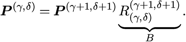 $$ \begin{align*} \boldsymbol{P}^{(\gamma,\delta)} = \boldsymbol{P}^{(\gamma+1,\delta+1)} \underbrace{R_{(\gamma,\delta)}^{(\gamma+1,\delta+1)}}_B. \end{align*} $$
Thus we have the following generalized eigenvalue equation:
 $$ \begin{align*} A R_{(\alpha,\beta)}^{(\gamma,\delta)} = B R_{(\alpha,\beta)}^{(\gamma,\delta)} \Lambda, \end{align*} $$
where
 $\Lambda $
is the diagonal eigenvalue matrix with
 $\Lambda _{n,n} = n(n+\alpha +\beta +1)$
.
A normalization of the generalized eigenvectors is necessary since (4.4) determines the eigenvectors only up to a scaling. This can obtained by examining the leading coefficients of both families. For Jacobi polynomials, these are a ratio of Pochhammer symbols:
 $$ \begin{align*} (R_{(\alpha,\beta)}^{(\gamma,\delta)})_{n,n}= \dfrac{(n+\alpha+\beta+1)_n}{(n+\gamma+\delta+1)_n}, \end{align*} $$
which may be evaluated recursively.
4.6.2 The Laguerre–Laguerre connection problem
The Laguerre–Laguerre connection problem relates two families of Laguerre polynomials, that is,
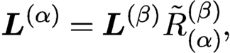 $$ \begin{align*} \boldsymbol{L}^{(\alpha)} = \boldsymbol{L}^{(\beta)} \tilde R_{(\alpha)}^{(\beta)}{,} \end{align*} $$
for some
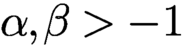 $\alpha ,\beta>-1$
. We have
 $$ \begin{align*} & [-x{\mathcal D}^2 + (x-\alpha-1){\mathcal D}] \boldsymbol{L}^{(\beta)} \\ & \quad= \boldsymbol{L}^{(\beta+1)} \underbrace{\bigl[-\tilde L_{(\beta+2)}^{(\beta+1)} \tilde D_{(\beta)}^{(\beta+2)} + (\tilde X_{(\beta+1)} - (\alpha+1) I ) \tilde D_{(\beta)}^{(\beta+1)} \bigr] }_A {,} \end{align*} $$
while the right-hand side is
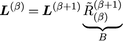 $$ \begin{align*} \boldsymbol{L}^{(\beta)} = \boldsymbol{L}^{(\beta+1)} \underbrace{\tilde R_{(\beta)}^{(\beta+1)}}_B \end{align*} $$
and
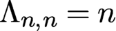 $\Lambda _{n,n} = n$
. For Laguerre polynomials, the normalization of the connection coefficients is trivial as
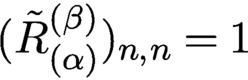 $(\tilde R_{(\alpha )}^{(\beta )})_{n,n} = 1$
.
4.6.3 The ultraspherical–ultraspherical connection problem
For the ultraspherical–ultraspherical connection problem, that is,
 $$ \begin{align*} \boldsymbol{C}^{(\lambda)} = \boldsymbol{C}^{(\mu)} R_{(\lambda)}^{(\mu)}, \quad {\text{{for} } \lambda, \mu> -1/2, \ \lambda, \mu \neq 0,} \end{align*} $$
we note that (4.4) becomes
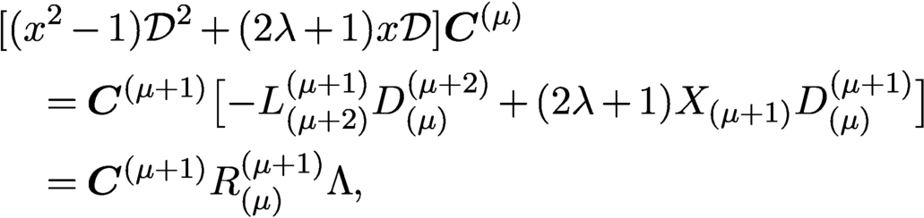 $$ \begin{align*} & [(x^2-1){\mathcal D}^2 + (2\lambda+1)x{\mathcal D}] \boldsymbol{C}^{(\mu)} \\ & \quad =\boldsymbol{C}^{(\mu+1)} \bigl[-L_{(\mu+2)}^{(\mu+1)} D_{(\mu)}^{(\mu+2)} + (2\lambda + 1) X_{(\mu+1)} D_{(\mu)}^{(\mu+1)}\bigr] \\ &\quad = \boldsymbol{C}^{(\mu+1)} R_{(\mu)}^{(\mu+1)} \Lambda, \end{align*} $$
where
 $\Lambda _{n,n} = n(n+2\lambda )$
. For ultraspherical polynomials, the normalization of the connection coefficients is given by the ratio of Pochhammer symbols:
 $$ \begin{align*} (R_{(\lambda)}^{(\mu)})_{n,n} = (\lambda)_n/ (\mu)_n, \end{align*} $$
which again may be evaluated recursively.
4.6.4 The triangular-banded divide-and-conquer scheme
We consider a divide-and-conquer scheme to obtain a structured form of the generalized eigenvectors of a banded upper-triangular Sylvester equation
 $$ \begin{align*} AV = BV\Lambda. \end{align*} $$
Since A and B are upper-triangular matrices, it is clear that the generalized eigenvalues are the ratios of the diagonal entries of the matrices. That is,
 $\Lambda _{i,i} = A_{i,i}/B_{i,i}$
for
 $i\geq 1$
.
In what follows, we consider the
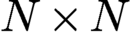 $N \times N$
truncation of this system. That is, we consider
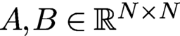 $A , B \in {\mathbb R}^{N \times N}$
. Let
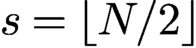 $s = \lfloor {N}/{2}\rfloor $
and let b be the upper bandwidth of both A and B. We suppose that V has the form
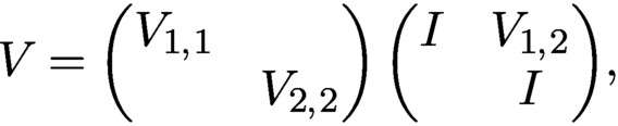 $$ \begin{align*} V = \begin{pmatrix} V_{1,1}\\ & V_{2,2}\end{pmatrix}\begin{pmatrix} I & V_{1,2}\\ & I\end{pmatrix}\!, \end{align*} $$
where
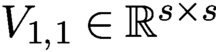 $V_{1,1}\in {\mathbb R}^{s\times s}$
,
 $V_{1,2}\in {\mathbb R}^{s\times (N-s)}$
and
 $V_{2,2}\in {\mathbb R}^{(N-s)\times (N-s)}$
are all roughly the same size. Block-dividing A, B and
 $\Lambda $
, we have
 $$ \begin{align*} \begin{pmatrix} A_{1,1} & A_{1,2}\\ & A_{2,2}\end{pmatrix}\begin{pmatrix} V_{1,1} & V_{1,1}V_{1,2}\\ & V_{2,2}\end{pmatrix} = \begin{pmatrix} B_{1,1} & B_{1,2}\\ & B_{2,2}\end{pmatrix}\begin{pmatrix} V_{1,1}\Lambda_1 & V_{1,1}V_{1,2}\Lambda_2\\ & V_{2,2}\Lambda_2\end{pmatrix}\!. \end{align*} $$
This decomposes into three subproblems
 $A_{1,1}V_{1,1} = B_{1,1}V_{1,1}\Lambda _1$
,
 $A_{2,2}V_{2,2} = B_{2,2}V_{2,2}\Lambda _2$
and
 $$ \begin{align*} A_{1,1}V_{1,1}V_{1,2} + A_{1,2}V_{2,2} = B_{1,1}V_{1,1}V_{1,2}\Lambda_2 + B_{1,2}V_{2,2}\Lambda_2. \end{align*} $$
This last equation is a Sylvester matrix equation for the block
 $V_{1,2}$
.
Supposing that
 $V_{1,1}^{-1} B_{1,1}^{-1} A_{1,1}V_{1,1} = \Lambda _1$
, the matrix equation can be cast into the following form:
 $$ \begin{align*} \Lambda_1V_{1,2} - V_{1,2}\Lambda_2 = V_{1,1}^{-1}B_{1,1}^{-1} (B_{1,2}V_{2,2}\Lambda_2 - A_{1,2}V_{2,2}). \end{align*} $$
Since A and B are banded with an upper bandwidth of b, it follows that
 $A_{1,2}$
and
 $B_{1,2}$
are matrices with only a small number of non-zero entries, arranged in a lower-triangular fashion in their bottom left corners. Thus the matrix–matrix product
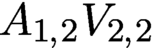 $A_{1,2}V_{2,2}$
results in a rank-b matrix with non-zero entries only in the last b rows. Similarly, due to the zero pattern in the matrix
 $A_{1,2}V_{2,2} - B_{1,2}V_{2,2}\Lambda _2$
, only the last b columns of
 $B_{1,1}^{-1}$
are needed, which are calculated with back-substitution using the last b columns of the
 $s\times s$
identity. We represent this block as the outer product of an
 $s\times b$
matrix X and a
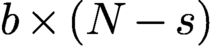 $b\times (N-s)$
matrix Y,
 $$ \begin{align*} V_{1,1}^{-1}B_{1,1}^{-1} (A_{1,2}V_{2,2} - B_{1,2}V_{2,2}\Lambda_2) =: XY^{\top}. \end{align*} $$
To conquer this problem, we examine the solution component-wise,
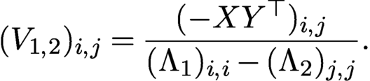 $$ \begin{align*} (V_{1,2})_{i,j} = \dfrac{(-XY^{\top})_{i,j}}{(\Lambda_1)_{i,i} - (\Lambda_2)_{j,j}}. \end{align*} $$
If we use the following notation to denote a Cauchy matrix generated by two vectors
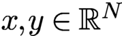 $x,y\in {\mathbb R}^N$
,
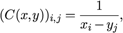 $$ \begin{align*} (C(x,y))_{i,j} = \dfrac{1}{x_i - y_j}, \end{align*} $$
then
 $V_{1,2}$
is the Hadamard product of a finite-rank matrix
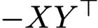 $-XY^{\top }$
and a Cauchy matrix
 $C(\operatorname {diag}{(\Lambda _1)}, \operatorname {diag}{(\Lambda _2)})$
. This can be expressed as a sum of diagonal scalings of the same Cauchy matrix,
 $$ \begin{align*} V_{1,2} = -\sum_{k=1}^b \operatorname{diag}{(X_{:,k})} C(\operatorname{diag}{(\Lambda_1)}, \operatorname{diag}{(\Lambda_2)}) \operatorname{diag}{(Y_{:,k})}. \end{align*} $$
Due to the separation of eigenvalues, the Cauchy matrices can be approximated, to within
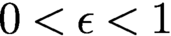 $0<\epsilon <1$
, by a matrix of rank
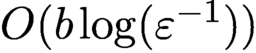 ${O} (b\log (\varepsilon ^{-1}))$
.
The structured form of the generalized eigenvectors permits inversion and transposition with the same computational complexity. We have
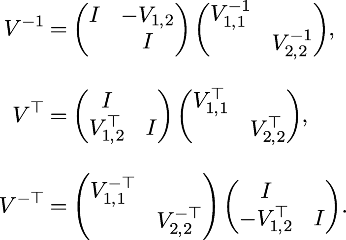 $$ \begin{align*} V^{-1} & = \begin{pmatrix} I & -V_{1,2}\\ & I\end{pmatrix}\begin{pmatrix} V_{1,1}^{-1}\\ & V_{2,2}^{-1}\end{pmatrix}\!,\\[10pt] V^{\top} & = \begin{pmatrix} I\\ V_{1,2}^{\top} & I\end{pmatrix}\begin{pmatrix} V_{1,1}^{\top}\\ & V_{2,2}^{\top}\end{pmatrix}\!,\\[10pt] V^{-\top} & = \begin{pmatrix} V_{1,1}^{-\top}\\ & V_{2,2}^{-\top}\end{pmatrix} \begin{pmatrix} I\\ -V_{1,2}^{\top} & I\end{pmatrix}\!. \end{align*} $$
Tables 4.2 and 4.3 show the timings and memory usage in single and double precision using the general-purpose algorithm introduced above. The timings demonstrate the quasi-linear complexity of the algorithm as well as its high accuracy.
Calculation times, memory requirements and error of the Chebyshev–Legendre transform (and back), the archetype of the measure-perturbing connection problem, in single precision.
 $s_d$
stands for the memory requirements of a dense
 $N\times N$
matrix,
 $s_p$
stands for the memory requirements of the pre-computations,
 $t_p$
stands for the pre-computation time,
 $t_e$
stands for the execution time, averaged over ten trials, and
 $\epsilon _2$
stands for the
 $2$
-norm relative error in transforming the coefficients
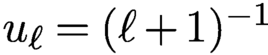 $u_{\ell } = (\ell +1)^{-1}$
, for
 $\ell = 0,\ldots ,N-1$
, forward and backward over the ten trials.
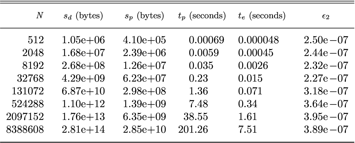
Calculation times, memory requirements and error of the Chebyshev–Legendre transform (and back), the archetype of the measure-perturbing connection problem, in double precision.
 $s_d$
stands for the memory requirements of a dense
 $N\times N$
matrix,
 $s_p$
stands for the memory requirements of the pre-computations,
 $t_p$
stands for the pre-computation time,
 $t_e$
stands for the execution time, averaged over ten trials, and
 $\epsilon _2$
stands for the
 $2$
-norm relative error in transforming the coefficients
 $u_{\ell } = 1/(\ell +1)$
, for
 $\ell = 0,\ldots ,N-1$
, forward and backward over the ten trials.
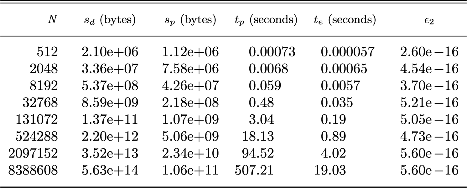
4.6.5 Words of caution
Not every measure-perturbing connection problem is well-conditioned. The structured form of the upper-triangular generalized eigenvectors allows for the following lower bound on the
 $2$
-norm condition number:
 $$ \begin{align*} \operatorname{cond}_2(V) := \|V\|_2{\|V^{-1}\|}_2 \geq \rho(V)\rho(V^{-1}), \end{align*} $$
where
 $\rho (V)$
is the spectral radius of V. This lower bound is equal to the ratio of largest to smallest absolute diagonal entries. An upper bound of the condition number can be given in terms of the Frobenius norm:
 $$ \begin{align*} \|V\|_2 \le \|V\|_F \le \sqrt{({\|V_{1,1}\|}_F^2+{\|V_{2,2}\|}_F^2)(N+{\|V_{1,2}\|}_F^2)}. \end{align*} $$
There are analogous upper and lower bounds for
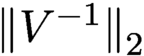 ${\|V^{-1}\|}_2$
.
Keiner (Reference Keiner2008) uses the lower bound on the condition number to determine when to subdivide the ultraspherical–ultraspherical connection problem into integer substeps between ultraspherical parameters
 $\lambda $
and
 $\mu $
and the fractional remainder. This analysis also translates to analogous results for Jacobi–Jacobi and Laguerre–Laguerre connection problems (Keiner Reference Keiner2011). In all cases, it is best to use the banded connection problems for integer increments/decrements in the parameters until the remaining difference in any parameter is less than
 $1$
.
For semiclassical orthogonal polynomials, the degree dependence in the variable coefficients in the differential equations enters into the linear algebra as diagonal scalings of the columns of the matrices of generalized eigenvectors. For example, it can be shown that the associated Jacobi–Jacobi connection coefficients satisfy
 $$ \begin{align*} AV + BV\Lambda = CV\Omega, \end{align*} $$
where
 $\|A\|_2, \|\Omega \|_2 = O(N^4)$
,
 $\|B\|_2, \|\Lambda \|_2 = O(N^2)$
and
 $\|C\|_2 = O(1)$
. Thus each member of this three-term matrix equation is equally as important as the others as
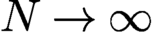 $N\to \infty $
. While numerical experiments suggest the off-diagonal blocks in the resulting matrix equations remain low-rank, further analysis is required to show that they can be rapidly approximated.
4.7 The measure-preserving connection problem
Measure-preserving connection problems are those between different bases that are orthogonal with respect to the same measure
 $\mu $
. We focus our attention on weighted orthogonal polynomial expansions. For example, the weighted orthonormal Jacobi polynomials
 $\boldsymbol {\hat P}^{(2,2)} := (1-x^2) \boldsymbol {P}^{(2,2)} M_{(2,2)}^{-1/2}$
are orthonormal with respect to
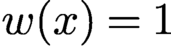 $w(x) = 1$
on
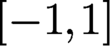 $[-1,1]$
, as are the normalized Legendre polynomials
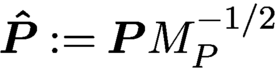 $\boldsymbol {\hat P} := \boldsymbol {P} M_P^{-1/2}$
. That is,
 $$ \begin{align*} \boldsymbol{\hat P}^{\top} \boldsymbol{\hat P} & = M_P^{-1/2} M_P M_P^{-1/2} = I, \\ (\boldsymbol{\hat P}^{(2,2)})^{\top} \boldsymbol{\hat P}^{(2,2)} & = M_{(2,2)}^{-1/2} (\boldsymbol{P}^{(2,2)})^{\top} (1-x^2)^2 \boldsymbol{P}^{(2,2)} M_{(2,2)}^{-1/2} = I. \end{align*} $$
Thus we aim to understand the connection problem
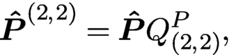 $$ \begin{align*} \boldsymbol{\hat P}^{(2,2)} = \boldsymbol{\hat P} Q_{(2,2)}^P, \end{align*} $$
where we use the notation Q in place of C to emphasize that it is an orthogonal transformation. Therefore, a measure-preserving transform is equivalent to a matrix–vector product involving an orthogonal matrix. It is natural to view
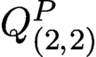 $Q_{(2,2)}^P$
(and other measure-preserving transforms) as a product of Givens rotations.
The measure-preserving connection problem is an important pathway to spherical harmonic synthesis and analysis as spherical harmonics involve the associated Legendre polynomials
 $$ \begin{align*} Y_\ell^m(\theta,\varphi) = \sqrt{\dfrac{\ell+{1}/{2}}{2\pi}\dfrac{(\ell-m)!}{(\ell+m)!}} P_\ell^m(\cos\theta) \,{\mathrm{e}}^{{\mathrm i} m \varphi}{.} \end{align*} $$
Over the past twenty years, there has been substantial progress in the construction and implementation of a fast spherical harmonic transform. Driscoll, Healy Jr and Rockmore (Reference Driscoll, Healy and Rockmore1997) introduced a procedure based on the so-called split-Legendre functions for constructing fast transforms for synthesis and analysis of spherical harmonics. In infinite-precision arithmetic, their algorithm is exact. However, their floating-point error analysis of the apparatus suggests the possibility of exponential growth in the error as m increases.
A few years after Driscoll et al. (Reference Driscoll, Healy and Rockmore1997), several groups including Potts, Steidl and Tasche (Reference Potts, Steidl and Tasche1998), Suda and Takami (Reference Suda and Takami2002), Healy Jr, Rockmore, Kostelec and Moore (Reference Healy, Rockmore, Kostelec and Moore2003) and Kunis and Potts (Reference Kunis and Potts2003) sought more stable strategies and efficiency improvements on the original scheme.
In an approach that generalizes the use of asymptotic formulas to accelerate the synthesis and analysis of Legendre polynomials, Mohlenkamp (Reference Mohlenkamp1999) used WKBJ asymptotic expansions of associated Legendre functions to accelerate the spherical harmonic transform. In addition to an asymptotically fast algorithm with predicted complexity
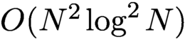 $O(N^{2}\log ^{2} N)$
, Mohlenkamp also develops an intermediate transform with complexity
 $O(N^{5}/2\log N)$
.
In the same spirit as the measure-perturbing problems of Section 4.6, asymptotically fast algorithms with
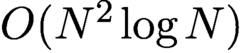 $O({N^2\log N})$
complexity have been developed by Rokhlin and Tygert (Reference Rokhlin and Tygert2006) based on a divide-and-conquer approach applied to a discretization of the differential equation satisfied by the associated Legendre functions. This is then accelerated further by the FMM. While this was the first asymptotically fast algorithm with asymptotically low pre-computation, it is only predicted to outperform other algorithms for absurdly large degrees.
Tygert continued to develop alternative spherical harmonic transforms by accelerating the direct synthesis and analysis (Tygert Reference Tygert2008) via divide-and-conquer of the Jacobi operators combined with a re-interpolation from Gauss–Jacobi nodes to the Gauss–Legendre grid for every associated Legendre order. He also developed an alternative approach based on compressing synthesis and analysis by the butterfly algorithm (Tygert Reference Tygert2010a ).
Notwithstanding this impressive body of literature, there are still improvements to be made. As a testament to this, some of the best software currently available for spherical harmonics is based on direct synthesis and analysis at Gaussian or equiangular grids (Schaeffer Reference Schaeffer2013, Reinecke and Seljebotn Reference Reinecke and Seljebotn2013, Ishioka Reference Ishioka2018) with
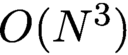 $O({N^3})$
complexity. One main bottleneck in making asymptotically fast transforms practical is the significant memory requirements in the storage of pre-computed data structures.
In light of these difficulties, Slevinsky (Reference Slevinsky2019) shows that (1) the neighbouring associated Legendre connection problem may be factored as a product of Givens rotations, and (2) the butterfly algorithm may also be applied to the connection problem. These two features offer improved backward stability of the connection problem, enable skeletonization of the pre-computation and provide insight on a rank property by relating connection coefficients to Fourier integral operators. A more vigorous skeletonization procedure is proposed in Slevinsky (Reference Slevinsky and Olver2017), which offers the complexity of
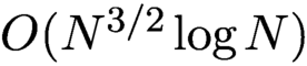 $O({N^{{3}/{2}}\log N})$
as a pre-computation cost in exchange for a modest increase in the execution complexity over the Rokhlin and Tygert (Reference Rokhlin and Tygert2006) scheme. With these results in hand, the question of making asymptotically fast transforms accessible at reasonably low degrees is no longer mathematical, but rather one of software. Our current progress in this endeavour is an open-source implementation, freely available in C (Slevinsky Reference Slevinsky2018a
) and Julia (Slevinsky Reference Slevinsky2016).
Remark 4.5. If an orthogonal polynomial appears with a tilde on top, then this implies standard orthonormalization with respect to its Hilbert space. The so-called neighbouring connection problems are based on a data-sparse factorization of connection coefficients. That is, rather than using recurrence relations to evaluate orthogonal polynomials, we convert their expansions using sequences of Givens rotations. Heuristically speaking, this procedure is more accurate because Givens rotations preserve Euclidean lengths, while recurrence relations do not.
Let
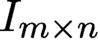 $I_{m\times n}$
denote the
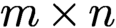 $m \times n$
rectangular identity matrix with ones on the main diagonal and zeros everywhere else.
4.7.1 The neighbouring connection problem
For any
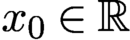 $x_0\in {\mathbb R}$
, let
 $(x-x_0)\varphi _n(x)$
and
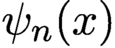 $\psi _n(x)$
be two families of orthonormal polynomials with respect to
 $\mu $
. The connection coefficients allow us to compute the expansion
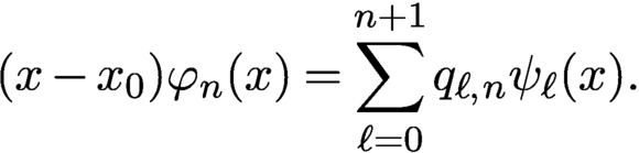 $$ \begin{align*} (x-x_0)\varphi_n(x) = \sum_{\ell=0}^{n+1} q_{\ell,n} \psi_\ell(x). \end{align*} $$
As columns of the connection coefficients are mutually orthonormal, we may factor the principal rectangular finite sections as a product of
 $n+1$
Givens rotations, the proof of which is by the
 $QR$
factorization of a rectangular matrix with zeros below the first sub-diagonal.
Let
 $G_n$
denote the real Givens rotation:
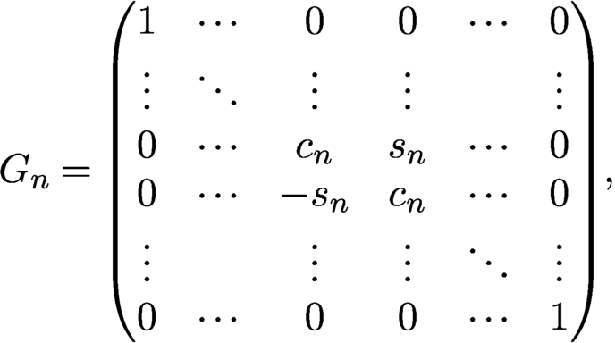 $$ \begin{align*} G_n = \begin{pmatrix} 1 & \cdots & 0 & 0 & \cdots & 0\\ \vdots & \ddots & \vdots & \vdots & & \vdots\\ 0 & \cdots & c_n & s_n & \cdots & 0\\ 0 & \cdots & -s_n & c_n & \cdots & 0\\ \vdots & & \vdots & \vdots & \ddots & \vdots\\ 0 & \cdots & 0 & 0 & \cdots & 1\\ \end{pmatrix}\!, \end{align*} $$
where
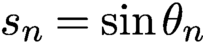 $s_n = \sin \theta _n$
and
 $c_n = \cos \theta _n$
, for some
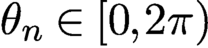 $\theta _n\in [0,2\pi )$
, are in the intersections of the nth and
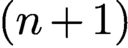 $(n+1)$
st rows and columns, embedded in the identity of a conformable size.
Theorem 4.6. The principal rectangular section of connection coefficients
 $Q \in {\mathbb R}^{(n+2)\times (n+1)}$
between
 $(x-x_0)\varphi _n(x)$
and
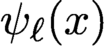 $\psi _\ell (x)$
may be represented via the product of
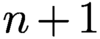 $n+1$
Givens rotations,
 $$ \begin{align*} Q = G_0\cdots G_n I_{(n+2)\times(n+1)}, \end{align*} $$
where the sines and cosines for the Givens rotations are given by
 $$ \begin{align*} {s_n = -q_{n+1,n}\quad\text{and}\quad c_n = \sqrt{1-q_{n+1,n}^2}.} \end{align*} $$
By relating the sines and the cosines to the highest connection coefficient of each column, they may be readily determined by comparing the coefficients of the highest powers of x.
For Jacobi polynomials, two special values of
 $x_0$
are
 $\pm 1$
, as both families may be identified as Jacobi polynomials with different but related parameters.
Corollary 4.7. The matrix of connection coefficients
 $Q^{(\alpha ,\beta )}\! \in \mathbb {R}^{(n+2)\times (n+1)}$
between
 $(1-x)\tilde {P}_n^{(\alpha +2,\beta )}(x)$
and
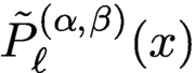 $\tilde {P}_{\ell }^{(\alpha ,\beta )}(x)$
may be represented via the product of
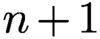 $n+1$
Givens rotations where the sines and cosines for the Givens rotations are given by
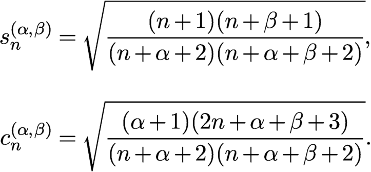 $$ \begin{align*} s_n^{(\alpha,\beta)} & = \sqrt{\dfrac{(n+1)(n+\beta+1)}{(n+\alpha+2)(n+\alpha+\beta+2)}},\\[10pt] c_n^{(\alpha,\beta)} & = \sqrt{\dfrac{(\alpha+1)(2n+\alpha+\beta+3)}{(n+\alpha+2)(n+\alpha+\beta+2)}}. \end{align*} $$
Since
 $P_n^{(\alpha ,\beta )}(-x) = (-1)^n P_n^{(\beta ,\alpha )}(x)$
, the connection coefficients between
 $(1+x)\tilde {P}_n^{(\alpha ,\beta +2)}(x)$
and
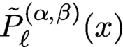 $\tilde {P}_{\ell }^{(\alpha ,\beta )}(x)$
are easily obtained by reversing the roles of
 $\alpha $
and
 $\beta $
above and negating the sines.
For Laguerre polynomials, a special value of
 $x_0$
is
 $0$
, for the same reason.
Corollary 4.8. The matrix of connection coefficients
 $Q^{(\alpha )} \in \mathbb {R}^{(n+2)\times (n+1)}$
between
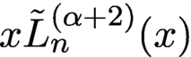 $x\tilde {L}_n^{(\alpha +2)}(x)$
and
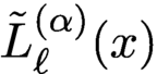 $\tilde {L}_{\ell }^{(\alpha )}(x)$
may be represented via the product of
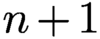 $n+1$
Givens rotations where the sines and cosines for the Givens rotations are given by
 $$ \begin{align*} s_n^{(\alpha)} = \sqrt{\dfrac{n+1}{n+\alpha+2}},\quad c_n^{(\alpha)} = \sqrt{\dfrac{\alpha+1}{n+\alpha+2}}. \end{align*} $$
If
 $\mu $
admits families of orthogonal polynomials that have even–odd symmetry, i.e.
 $\psi _n(-x) = (-1)^n\psi _n(x)$
, then the connection coefficients between
 $(x^2-x_0^2)\varphi _n(x)$
and
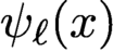 $\psi _\ell (x)$
respect this symmetry through a chessboard pattern of zeros which is also observed in the Givens rotations.
Let
 $G_n$
denote the real Givens rotation
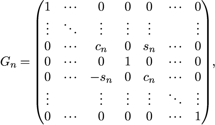 $$ \begin{align*} G_n = \begin{pmatrix} 1 & \cdots & 0 & 0 & 0 & \cdots & 0\\ \vdots & \ddots & \vdots & \vdots & \vdots & & \vdots\\ 0 & \cdots & c_n & 0 & s_n & \cdots & 0\\ 0& \cdots & 0 & 1 & 0 & \cdots & 0\\ 0 & \cdots & -s_n & 0 & c_n & \cdots & 0\\ \vdots & & \vdots & \vdots & \vdots & \ddots & \vdots\\ 0 & \cdots & 0 & 0 & 0 & \cdots & 1\\ \end{pmatrix}\!, \end{align*} $$
where the sines
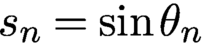 $s_n = \sin \theta _n$
and the cosines
 $c_n = \cos \theta _n$
, for some
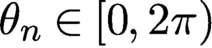 $\theta _n\in [0,\,2\pi )$
, are now in the intersections of the nth and
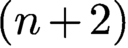 $(n+2)$
nd rows and columns, embedded in the identity of a conformable size.
Theorem 4.9. The principal rectangular section of connection coefficients
 $Q\in {\mathbb R}^{(n+3)\times (n+1)}$
between
 $(x^2-x_0^2)\varphi _n(x)$
and
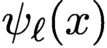 $\psi _\ell (x)$
may be represented via the product of
 $n+1$
Givens rotations,
 $$ \begin{align*} Q = G_0\cdots G_n I_{(n+3)\times(n+1)}, \end{align*} $$
where the sines and cosines for the Givens rotations are given by
 $$ \begin{align*} {s_n = -q_{n+2,n}\quad\text{and}\quad c_n = \sqrt{1-q_{n+2,n}^2}.} \end{align*} $$
For Jacobi polynomials with equal parameters, a special value of
 $x_0$
is
 $1$
.
Corollary 4.10. The matrix of connection coefficients
 $Q^{(\alpha )} \in \mathbb {R}^{(n+3)\times (n+1)}$
between
 $(1-x^2)\tilde {P}_n^{(\alpha +2,\alpha +2)}(x)$
and
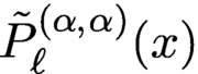 $\tilde {P}_\ell ^{(\alpha ,\alpha )}(x)$
may be represented via the product of
 $n+1$
Givens rotations, where the sines and cosines for the Givens rotations are given by
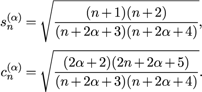 $$ \begin{align*} s_n^{(\alpha)} & = \sqrt{\dfrac{(n+1)(n+2)}{(n+2\alpha+3)(n+2\alpha+4)}},\\[2pt] c_n^{(\alpha)} & = \sqrt{\dfrac{(2\alpha+2)(2n+2\alpha+5)}{(n+2\alpha+3)(n+2\alpha+4)}}. \end{align*} $$
The representations for the Givens rotations of the neighbouring connection problems along with the representations of the sines and cosines as square roots of rationals ipso facto enables the design and implementation of backward stable direct algorithms (Slevinsky Reference Slevinsky2019, Algorithm 2.5).
Table 4.4 shows a full spherical harmonic synthesis and analysis compared with SHTns and ISPACK, two high-performance spherical harmonic libraries based on direct synthesis and analysis. Compare with Ishioka (Reference Ishioka2018, Table 2).
The
 $2$
-norm and
 $\infty $
-norm relative errors in a full spherical harmonic synthesis and analysis on an equiangular grid with pseudo-random expansion coefficients drawn from
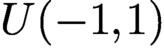 $U(-1,1)$
.
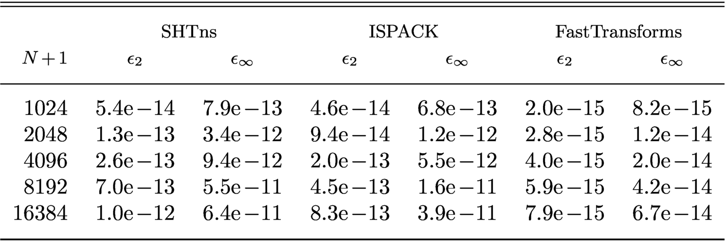
4.7.2 Associated Legendre functions and symmetric definite and banded generalized eigenvalue problems
For asymptotically fast transforms, we must consider more than the neighbouring connection problem. In this case, we would again like to exploit the differential eigenvalue problems satisfied by weighted orthonormal polynomials. A hat on top of a symbol denotes that the orthonormal polynomials are weighted by the square root of the orthonormality weight. For example, the weighted Jacobi polynomials satisfy
 $$ \begin{align*} \hat{P}_n^{(\alpha,\beta)}(x) := (1-x)^{{\alpha}/{2}}(1+x)^{{\beta}/{2}} \tilde{P}_n^{(\alpha,\beta)}(x). \end{align*} $$
If
 $\beta =\alpha =m\in \mathbb {N}_0$
, then it is well known that these weighted Jacobi polynomials are proportional to associated Legendre functions, which are the latitudinal component of spherical harmonics.
Normalized associated Legendre functions of degree
 $\ell $
and order m are eigenfunctions of the following linear differential equation:
 $$ \begin{align} (1-x^2)(-{\mathcal D}) [(1-x^2){\mathcal D}\tilde{P}_\ell^m(x)] + m^2\tilde{P}_\ell^m(x) \!=\! \ell(\ell+1)(1-x^2)\tilde{P}_\ell^m(x), \!\!\!\!\!\!\quad |m| \!\le\! \ell, \end{align} $$
which we write in quasimatrix notation as
 $$ \begin{align*} (1-x^2)(-{\mathcal D})(1-x^2){\mathcal D} \boldsymbol{P}^m + m^2 \boldsymbol{P}^m = \boldsymbol{P}^m (\underbrace{I - X_m^2}_M) \Lambda_m \end{align*} $$
for
 $X_m$
defined in (A.1). This means that M is a pentadiagonal, symmetric and positive definite matrix. If we write
 $\boldsymbol {P}^\nu = \boldsymbol {P}^m Q_\nu ^m,$
then we find that
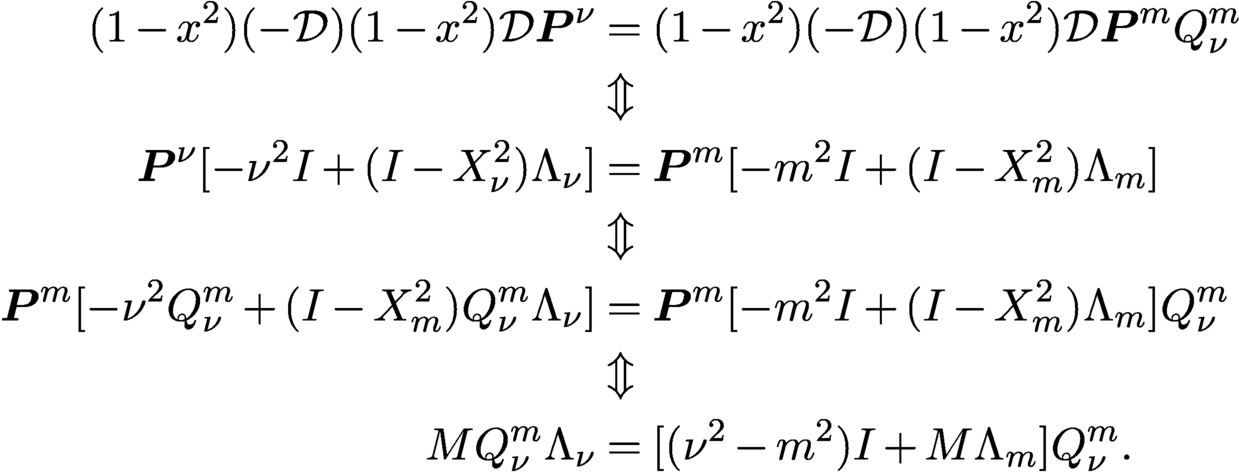 $$ \begin{align*} (1-x^2)(-{\mathcal D})(1-x^2){\mathcal D} \boldsymbol{P}^\nu &= (1-x^2)(-{\mathcal D})(1-x^2){\mathcal D} \boldsymbol{P}^m Q_\nu^m \\ &\Updownarrow\\ \boldsymbol{P}^\nu [-\nu^2 I + (I - X_\nu^2) \Lambda_\nu ] &=\boldsymbol{P}^m [-m^2 I + (I - X_m^2) \Lambda_m ] \\ &\Updownarrow\\ \boldsymbol{P}^m [-\nu^2 Q_\nu^m + (I - X_m^2) Q_\nu^m \Lambda_\nu ] &=\boldsymbol{P}^m [-m^2 I + (I - X_m^2) \Lambda_m ] Q_\nu^m \\ &\Updownarrow \\ M Q_\nu^m \Lambda_\nu & = [(\nu^2-m^2) I +M \Lambda_m ] Q_\nu^m. \end{align*} $$
That is, we have
 $$ \begin{align*} [M \Lambda_m + (\nu^2 -m^2) I] Q_\nu^m = M Q_\nu^m \Lambda_\nu. \end{align*} $$
Unfortunately, the symmetry in M is destroyed by the column scaling in
 $\Lambda $
. Rokhlin and Tygert (Reference Rokhlin and Tygert2006) realized that the generalized eigenvalue problem is symmetrized when multiplied by
 $M^{-1}$
from the left, resulting in
 $$ \begin{align*} [\Lambda_m + (\nu^2-m^2)M^{-1} ] Q_\nu^m = Q_\nu^m \Lambda_\nu. \end{align*} $$
This symmetric diagonal-plus-semiseparable regular eigenvalue problem is the starting point for their fast spherical harmonic transform (Rokhlin and Tygert Reference Rokhlin and Tygert2006). The FMM accelerates the divide-and-conquer algorithm for symmetric diagonal-plus-semiseparable eigenvalue problems developed by Chandrasekaran and Gu (Reference Chandrasekaran and Gu2004).
An alternative to multiplication by
 $M^{-1}$
is to use the Cholesky factorization and a change of bases. If we take the Cholesky factorization of
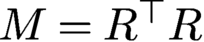 $M = R^{\top } R$
, consider new generalized eigenvectors
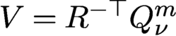 $V = R^{-\top } Q_\nu ^m$
and multiply by
 $R^{-\top }$
from the left, then we transform the problem into the following:
 $$ \begin{align*} [R\Lambda_m R^{\top} + (\nu^2-m^2)I]V = RR^{\top} V \Lambda_\nu. \end{align*} $$
This generalized eigenvalue problem is symmetric definite and pentadiagonal,Footnote
5
allowing for a fast spectral decomposition (Borges and Gragg Reference Borges, Gragg, Reichel, Ruttan and Varga1993, Gu and Eisenstat Reference Gu and Eisenstat1995). Furthermore, the generalized eigenvectors V are
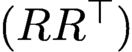 $(RR^{\top })$
-orthogonal, in the sense that
 $$ \begin{align*} V^{\top} RR^{\top} V = I. \end{align*} $$
In Appendix A of Slevinsky (Reference Slevinsky and Olver2017), explicit formulas are given for the Cholesky factor R and the products
 $RR^{\top }$
and
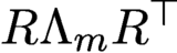 $R\Lambda _mR^{\top }$
.
In this case, the problem is pentadiagonal, but the zero pattern ensures that it may be decoupled into two symmetric definite and tridiagonal problems.
4.7.3 Weighted normalized Jacobi polynomials
The construction for associated Legendre polynomials is also possible for other weighted Jacobi transforms, arising in fast transforms for OPs. The weighted normalized Jacobi polynomials
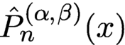 $\hat {P}_n^{(\alpha ,\beta )}(x)$
are eigenfunctions of the following linear differential equation:
 $$ \begin{align} & (1-x^2)(-{\mathcal D})[(1-x^2){\mathcal D}\hat{P}_n^{(\alpha,\beta)}(x)] \notag \\ &~~~~ +\biggl(\biggl(\displaystyle \frac{\alpha}{2}\biggr)^2(1+x)^2+\biggl(\displaystyle \frac{\beta}{2}\biggr)^2(1-x)^2-\displaystyle \frac{(\alpha\beta+\alpha+\beta)}{2}(1-x^2)\biggr)\hat{P}_n^{(\alpha,\beta)}(x)\nonumber\\ &~~ = n(n+\alpha+\beta+1)(1-x^2)\hat{P}_n^{(\alpha,\beta)}(x). \end{align} $$
This Sturm–Liouville problem is the two-parameter generalization of (4.5) for associated Legendre functions. When we view multiplication by
 $1\pm x$
as an operator acting on the basis of weighted normalized Jacobi polynomials, we can identify that certain terms in (4.6) are symmetric positive definite and pentadiagonal matrices.
If we expand the weighted normalized Jacobi polynomials of parameters
 $\gamma $
and
 $\delta $
in the basis of weighted normalized Jacobi polynomials of parameters
 $\alpha $
and
 $\beta $
, that is,
 $$ \begin{align*} \hat{\boldsymbol{P}}^{(\gamma,\delta)}(x) = \hat{\boldsymbol{P}}^{(\alpha,\beta)}(x) Q_{(\gamma,\delta)}^{(\alpha,\beta)}, \end{align*} $$
then we may rewrite the Sturm–Liouville problem in (4.6) symbolically as
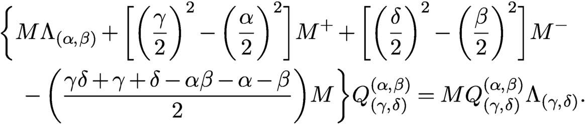 $$ \begin{align} & \bigg\{M \Lambda_{(\alpha,\beta)} + \bigg[\bigg(\displaystyle \frac{\gamma}{2}\bigg)^2-\bigg(\displaystyle \frac{\alpha}{2}\bigg)^2\bigg]M^+ + \bigg[\bigg(\displaystyle \frac{\delta}{2}\bigg)^2-\bigg(\displaystyle \frac{\beta}{2}\bigg)^2\bigg]M^- \notag\\ &\quad -\bigg(\displaystyle \frac{\gamma\delta+\gamma+\delta-\alpha\beta-\alpha-\beta}{2}\bigg)M\bigg\} Q_{(\gamma,\delta)}^{(\alpha,\beta)} = M Q_{(\gamma,\delta)}^{(\alpha,\beta)} \Lambda_{(\gamma,\delta)}. \end{align} $$
Here we have
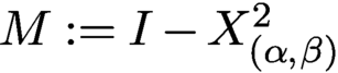 $M := I- X_{(\alpha ,\beta )}^2$
,
 $M^+ := (I+X_{(\alpha ,\beta )})^2$
,
 $M^-:= (I-X_{(\alpha ,\beta )})^2$
, and
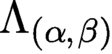 $\Lambda _{(\alpha ,\beta )}$
is the diagonal scaling of the basis by
 $n(n+\alpha +\beta +1)$
for
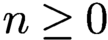 $n\ge 0$
.
Due to the orthonormal polynomial recurrence relation, all the multiplication operators may be derived analytically, and algorithms for their component-wise computation to high relative accuracy are described in Appendix B in Slevinsky (Reference Slevinsky and Olver2017).
If we let S denote the weighted sum of symmetric positive definite multiplication operators on the left-hand side of (4.7), then we have
 $$ \begin{align*} ( M \Lambda_{(\alpha,\beta)} + S ) Q_{(\gamma,\delta)}^{(\alpha,\beta)} = M Q_{(\gamma,\delta)}^{(\alpha,\beta)} \Lambda_{(\gamma,\delta)}, \end{align*} $$
where M is a symmetric positive definite and banded matrix,
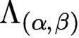 $\Lambda _{(\alpha ,\beta )}$
is diagonal and S is symmetric and banded. If we use the same strategy as for spherical harmonics, then we would take the Cholesky factorization of
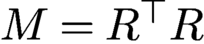 $M = R^{\top } R$
and rearrange to obtain
 $$ \begin{align} ( R\Lambda_{(\alpha,\beta)} R^{\top} + R^{-\top}SR^{\top} )V = RR^{\top} V\Lambda_{(\gamma,\delta)}. \end{align} $$
As before,
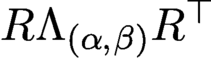 $R\Lambda _{(\alpha ,\beta )} R^{\top }$
is symmetric and banded and
 $RR^{\top }$
is symmetric positive definite and banded, but the new term
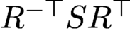 $R^{-\top }SR^{\top }$
is no longer a scalar multiple of the identity matrix (as for spherical harmonics). In fact, not much of its structure is apparent by this formulation.
To reveal the structure of
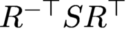 $R^{-\top }SR^{\top }$
, we make use of another property of our eigenproblem. Since M and S are multiplication operators with the same separable Hilbert spaces attached to the domain and range, they commute. That is,
 $MS = SM$
, or in terms of the commutator
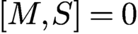 $[M,S] = 0$
. We use the commutator and the (formal) invertibility of M to write
 $S = MSM^{-1}$
, leading to the equivalent representation
 $$ \begin{align*} ( R\Lambda_{(\alpha,\beta)} R^{\top} + RSR^{-1} )V = RR^{\top} V \Lambda_{(\gamma,\delta)}. \end{align*} $$
By the Cholesky factorization, R is an upper-triangular and banded matrix. Thus
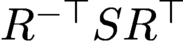 $R^{-\top }SR^{\top }$
has non-zero entries up to and including the second superdiagonal. Furthermore
 $$ \begin{align*} RSR^{-1} = (R^{-\top}S^{\top} R^{\top})^{\top} = (R^{-\top}SR^{\top})^{\top} = R^{-\top}SR^{\top}. \end{align*} $$
It turns out that
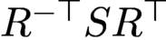 $R^{-\top }SR^{\top }$
in (4.8) is in fact a symmetric and banded matrix.
4.7.4 Weighted Laguerre polynomials
The weighted normalized Laguerre polynomials
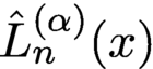 $\hat {L}_n^{(\alpha )}(x)$
are eigenfunctions of the linear differential equation
 $$ \begin{align*} x(-{\mathcal D})[x{\mathcal D} \hat{L}_n^{(\alpha)}(x)] + \displaystyle \frac{1}{4}(\alpha-x)^2 \hat{L}_n^{(\alpha)}(x) = \biggl(n+\displaystyle \frac{1}{2}\biggr)x\hat{L}_n^{(\alpha)}(x). \end{align*} $$
We may view M as multiplication by x, and
 $\Lambda $
as a diagonal scaling. When
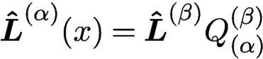 $\boldsymbol {\hat {L}}^{(\alpha )}(x)= \boldsymbol {\hat {L}}^{(\beta )} Q_{(\alpha )}^{(\beta )}$
, we again arrive at
 $$ \begin{align*} (M\Lambda + S) Q_{(\alpha)}^{(\beta)} = M Q_{(\alpha)}^{(\beta)} \Lambda, \end{align*} $$
where
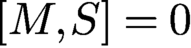 $[M,S]=0$
. Since M is a symmetric and positive definite matrix, this equation is symmetrizable by the same technique as above.
4.8 Symmetric definite and banded divide-and-conquer
We have shown that measure-preserving connection problems for weighted and orthonormalized classical orthogonal polynomials result in the symmetric definite and banded generalized eigenproblem of the form
 $$ \begin{align} AV = BV\Lambda,\quad V^{\top} B V = I. \end{align} $$
There are several significant contributions to the literature on divide-and-conquer for special types of eigenproblems, with special attention to rank-one symmetric modifications of known eigenproblems in the conquer step. This includes the seminal works of Bunch, Nielsen and Sorensen (Reference Bunch, Nielsen and Sorensen1978) and Cuppen (Reference Cuppen1981) and improvements to stability in Gu and Eisenstat (Reference Gu and Eisenstat1994). For the related symmetric arrowhead conquer step, this is also described in Gu and Eisenstat (Reference Gu and Eisenstat1995) and includes the observation that the FMM may accelerate an eigenmatrix–vector product. For the generalized eigenproblem, the tridiagonal case was described in Borges and Gragg (Reference Borges, Gragg, Reichel, Ruttan and Varga1993) with arrowhead divide-and-conquer and Elsner, Fasse and Langmann (Reference Elsner, Fasse and Langmann1997) with a symmetric rank-one modification. These algorithms have been adapted quite recently to the hierarchical semi-separable format (Vogel, Xia, Cauley and Balakrishnan Reference Vogel, Xia, Cauley and Balakrishnan2016). Here, we extend divide-and-conquer to the symmetric definite and banded generalized eigenvalue problem in (4.9).
Let
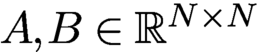 $A, B\in {\mathbb R}^{N\times N}$
, and let
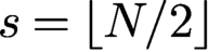 $s = \lfloor {N}/{2}\rfloor $
and
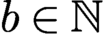 $b\in \mathbb {N}$
be the (symmetric) bandwidth of both A and B. We divide A and B conformably,
 $$ \begin{align*} A = \begin{pmatrix}A_1 & A_3^{\top}\\ A_3 & A_2\end{pmatrix}\!,\quad B = \begin{pmatrix}B_1 & B_3^{\top}\\ B_3 & B_2\end{pmatrix}\!, \end{align*} $$
where
 $$ \begin{align*} {A_1,B_1\in{\mathbb R}^{s\times s},\quad A_2,B_2\in{\mathbb R}^{(N-s)\times(N-s)} \quad\text{and}\quad A_3,B_3\in{\mathbb R}^{(N-s)\times s}.} \end{align*} $$
Since A and B are banded,
 $A_3$
and
 $B_3$
have the canonical decompositions
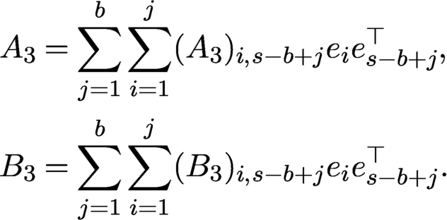 $$ \begin{align*} A_3 & = \sum_{j=1}^b\sum_{i=1}^j (A_3)_{i,s-b+j} e_i e_{s-b+j}^{\top},\\ B_3 & = \sum_{j=1}^b\sum_{i=1}^j (B_3)_{i,s-b+j} e_i e_{s-b+j}^{\top}. \end{align*} $$
Thus we may represent A and B as finite-rank perturbations of two divided problems of nearly half the original size. While there are a few choices to the finite-rank perturbations, in the context of an eigensolver, it is important to choose perturbations that are symmetric and favourable to the root-finder. We will now show that this is always possible.
If we define
 $$ \begin{align*} w_{i,j} = e_{i+s} + \widetilde{{\text{sgn}\,}}[(B_3)_{i,s-b+j}] e_{s-b+j},\quad \widetilde{{\text{ sgn}\,}}(x) = \begin{cases} 1 & x\ge0,\\ -1 & x < 0, \end{cases} \end{align*} $$
then A and B may be decomposed as
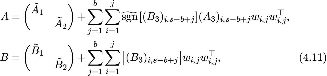 $$ \begin{align} A & = \begin{pmatrix} \tilde{A}_1\\ & \tilde{A}_2\end{pmatrix} + \sum_{j=1}^b\sum_{i=1}^j \widetilde{{\text{sgn}\,}}[(B_3)_{i,s-b+j}] (A_3)_{i,s-b+j} w_{i,j}w_{i,j}^{\top},\\ B & = \begin{pmatrix} \tilde{B}_1\\ & \tilde{B}_2\end{pmatrix} + \sum_{j=1}^b\sum_{i=1}^j {\big|(B_3)_{i,s-b+j}\big|} w_{i,j}w_{i,j}^{\top},\tag{4.11} \end{align} $$
where
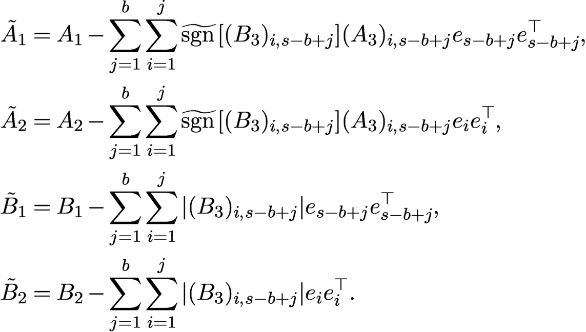 $$ \begin{align*} \tilde{A}_1 & = A_1 - \sum_{j=1}^b\sum_{i=1}^j \widetilde{{\text{sgn}\,}}[(B_3)_{i,s-b+j}] (A_3)_{i,s-b+j} e_{s-b+j}e_{s-b+j}^{\top},\\ \tilde{A}_2 & = A_2 - \sum_{j=1}^b\sum_{i=1}^j \widetilde{{\text{sgn}\,}}[(B_3)_{i,s-b+j}] (A_3)_{i,s-b+j} e_i e_i^{\top},\\ \tilde{B}_1 & = B_1 - \sum_{j=1}^b\sum_{i=1}^j {|(B_3)_{i,s-b+j}|} e_{s-b+j}e_{s-b+j}^{\top},\\ \tilde{B}_2 & = B_2 - \sum_{j=1}^b\sum_{i=1}^j {|(B_3)_{i,s-b+j}|} e_i e_i^{\top}. \end{align*} $$
Next, assume that the two subproblems have been solved, so that
 $$ \begin{align*} V_i^{\top} (\tilde{A}_i - \lambda\tilde{B}_i) V_i = D_i - \lambda I \quad\text{for } i = 1,2. \end{align*} $$
Then (4.10) and (4.11) are congruent to the
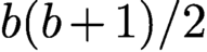 $b(b+1)/2$
-rank symmetric perturbation of the diagonal generalized eigenvalue problem. That is, there exist vectors
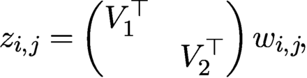 $$ \begin{align*} z_{i,j} = \begin{pmatrix} V_1^{\top}\\& V_2^{\top}\end{pmatrix}w_{i,j}\!, \end{align*} $$
so that
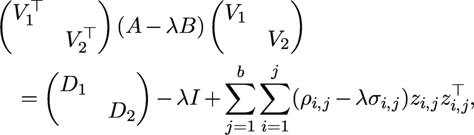 $$ \begin{align} & \begin{pmatrix} V_1^{\top}\\ & V_2^{\top}\end{pmatrix} (A-\lambda B) \begin{pmatrix} V_1\\ & V_2\end{pmatrix}\nonumber\\ & \quad = \begin{pmatrix} D_1\\ & D_2\end{pmatrix} - \lambda I + \sum_{j=1}^b\sum_{i=1}^j (\rho_{i,j}-\lambda \sigma_{i,j}) z_{i,j} z_{i,j}^{\top}, \end{align} $$
where
 $\rho _{i,j} = \widetilde {{\text{sgn}\,}}[(B_3)_{i,s-b+j}] (A_3)_{i,s-b+j}$
and
 $\sigma _{i,j} = {|(B_3)_{i,s-b+j}|} \ge 0$
.
In the conquer step, we must now solve the finite-rank symmetric perturbation of the diagonal generalized eigenvalue problem. This leads us to consider, in turn, the rank-one symmetric perturbation of the diagonal generalized eigenvalue problem, as the finite-rank case may be broken into a sequence of rank-one updates.
Based on (4.12), we consider the following generalized eigenvalue problem:
 $$ \begin{align} {(D + \rho zz^{\top})v = \lambda (I+\sigma zz^{\top})v,} \end{align} $$
where
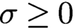 $\sigma \ge 0$
. The generalized eigenvalue problem may be deflated in the following three cases.
-
(1) If
$z_i=0$
, then
$\lambda _i = d_i$
is an eigenvalue with the corresponding eigenvector
$v=e_i$
. -
(2) If
$d_i = d_j$
for some pair of indices
$i\ne j$
, then a Givens rotation in the
$(i,j)$
-plane may be elected to introduce a zero in either
$z_i$
or
$z_j$
, while leaving the entries of D unchanged. Thus
$\lambda _i=d_i$
and we deflate as above. -
(3) If
$\tau := \rho /\sigma = d_i$
for some index i, then
$v = e_i$
is also an eigenvector with eigenvalue
$\lambda _i = \tau $
.
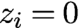
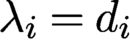
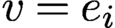
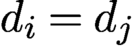


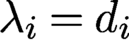

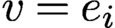
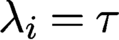
Therefore, by elementary deflation and permutation, we assume that the diagonal entries of D are increasing, i.e.
 $d_1\lt \cdots \lt d_N$
,
 $z_i\ne 0$
,
 $\tau \ne d_i$
, and that
 $z^{\top } z = 1$
. The scaling of z may be absorbed by the constants
 $\rho $
and
 $\sigma $
.
The following theorem was proved substantially by Elsner et al. (Reference Elsner, Fasse and Langmann1997), although they did not present the case where
 $\sigma \ge 0$
, which allows for an exact localization of all N eigenvalues.
Theorem 4.11. With all aforementioned assumptions, the generalized eigenvalues of (4.13) are roots of the secular equation
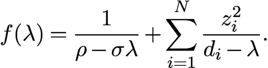 $$ \begin{align*} f(\lambda) = \dfrac{1}{\rho-\sigma \lambda} + \sum_{i=1}^N \dfrac{z_i^2}{d_i-\lambda}. \end{align*} $$
Let
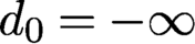 $d_0 = -\infty $
and
 $d_{N+1} = +\infty $
. Let
 $d_j < \tau (=\rho /\sigma ) < d_{j+1}$
for some
 $j = 0,\ldots ,N$
. Then there exists an eigenvalue in each interval
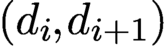 $(d_i,d_{i+1})$
for
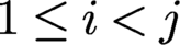 $1\le i\lt j$
, one in the interval
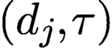 $(d_j, \tau )$
, another in the interval
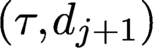 $(\tau , d_{j+1})$
and one more in each interval
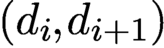 $(d_i,d_{i+1})$
for
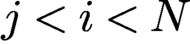 $j<i<N$
. Furthermore, the corresponding generalized eigenvector
 $v_j$
to
 $\lambda _j$
is given by
 $$ \begin{align} v_j = \biggl(\dfrac{z_1}{d_1-\lambda_j},\dfrac{z_2}{d_2-\lambda_j},\ldots,\dfrac{z_N}{d_N-\lambda_j}\biggr)^{\top}. \end{align} $$
The proof of this theorem relies on the observation that f is monotonically increasing, given that
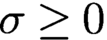 $\sigma \ge 0$
. In our choice of the finite-rank decomposition of A and B in (4.10) and (4.11), this is always true and we need never consider the monotonicity-breaking case of
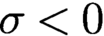 $\sigma <0$
.
By inspecting the equation
 $$ \begin{align*} v_j^{\top}(I+\sigma zz^{\top})v_j = \sum_{i=1}^N \dfrac{z_i^2}{(d_i-\lambda_j)^2} + \sigma\biggl(\sum_{i=1}^N\dfrac{z_i^2}{d_i-\lambda_j}\biggr)^2, \end{align*} $$
we are provided with a natural choice for the normalization
 $$ \begin{align} \tilde{v}_j = v_j/\sqrt{v_j^{\top}(I+\sigma zz^{\top})v_j}. \end{align} $$
Both (4.14) and (4.15) show the connection to diagonally scaled Cauchy and Coulomb matrices whose matrix–vector products may be accelerated by the FMM.
4.8.1 Computational issues
To find the roots of the secular equations, we use the cubically convergent algorithm described by Borges and Gragg (Reference Borges, Gragg, Reichel, Ruttan and Varga1993). This uses inverse rational interpolation for the function
 $$ \begin{align*} \Phi_i(\lambda) := p+\dfrac{q}{d_i-\lambda} + \dfrac{r}{d_{i+1}-\lambda}, \end{align*} $$
with suitable modifications for the eigenvalues in
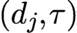 $(d_j,\tau )$
and
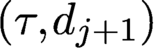 $(\tau ,d_{j+1})$
. The constants p, q and r are found by equating
 $\Phi _i^{(\nu )}(\lambda ^{(k)}) = f^{(\nu )}(\lambda ^{(k)})$
, for
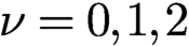 $\nu =0,1,2$
, and for every approximate eigenvalue
 $\lambda ^{(k)}$
, for
 $k=0,1,\ldots .$
The one root of
 $\Phi _i$
in the interval
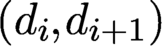 $(d_i, d_{i+1})$
is a solution of a quadratic equation.
It may occur that
 $\lambda _i$
is near one of the poles,
 $d_i$
or
 $d_{i+1}$
. In this case, it is advantageous to simulate an extended precision by representing
 $\lambda _i$
as the sum of
 $\lambda _i^{\mathrm hi}$
, defined by
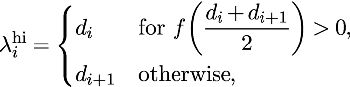 $$ \begin{align*} \lambda_i^{\mathrm{hi}} = \begin{cases} d_i & \text{for } f\biggl(\dfrac{d_i+d_{i+1}}{2}\biggr)> 0,\\[7pt] d_{i+1} & \text{otherwise}, \end{cases} \end{align*} $$
and
 $\lambda _i^{\mathrm lo}$
, defined by the difference
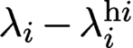 $\lambda _i - \lambda _i^{\mathrm hi}$
, though the difference is not explicitly computed. Instead, there is a shift of origin in the secular equation where difference is transferred to the diagonal entries
 $d_i$
. The numerical instability as the result of dividing by the difference of two nearly equal numbers is thereby eliminated.
Tables 4.5 and 4.6 show the timings and memory usage in single and double precision using the general-purpose algorithm introduced above. The timings help to demonstrate the quasi-linear complexity. The symmetric definite and banded divide-and-conquer approaches have a much higher pre-computation than the upper-triangular and banded divide-and-conquer for the measure-perturbing connection problem.
Calculation times, memory requirements and error of the associated Legendre transform
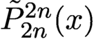 $\tilde {P}_{2n}^{2n}(x)$
to
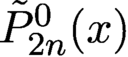 $\tilde {P}_{2n}^0(x)$
(and back), in single precision.
 $s_d$
stands for the memory requirements of a dense
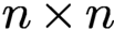 $n\times n$
matrix,
 $s_p$
stands for the memory requirements of the pre-computations,
 $t_p$
stands for the pre-computation time,
 $t_e$
stands for the execution time, averaged over ten trials, and
 $\epsilon _2$
stands for the
 $2$
-norm relative error in transforming the coefficient
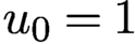 $u_0 = 1$
forward and backward over the ten trials.
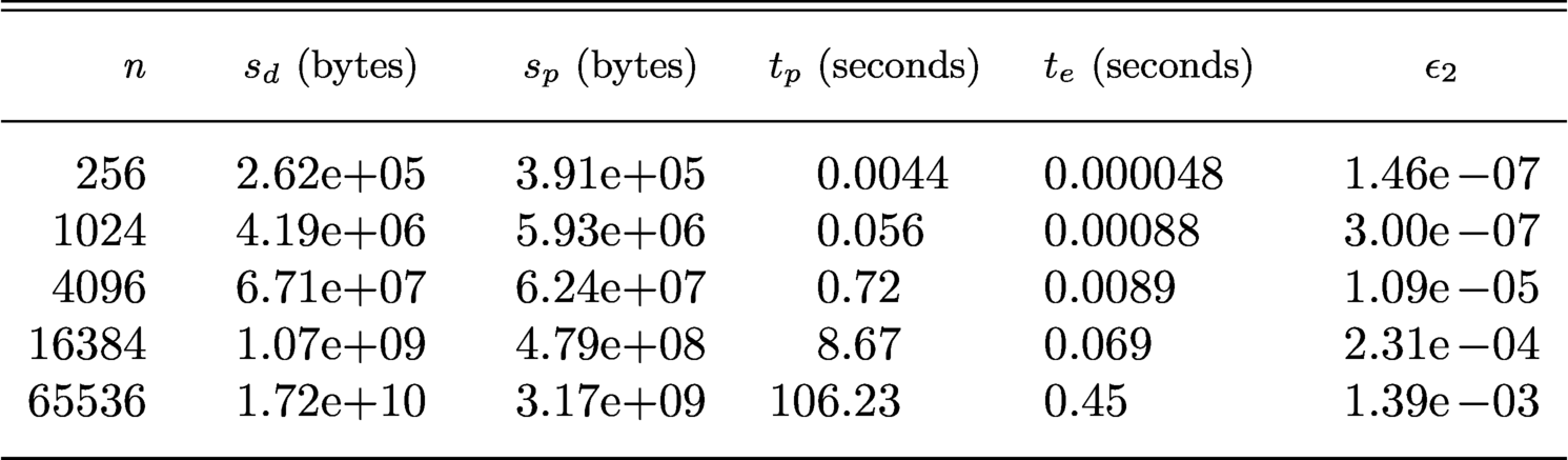
Calculation times, memory requirements and error of the associated Legendre transform
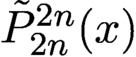 $\tilde {P}_{2n}^{2n}(x)$
to
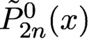 $\tilde {P}_{2n}^0(x)$
(and back), in double precision.
 $s_d$
stands for the memory requirements of a dense
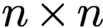 $n\times n$
matrix,
 $s_p$
stands for the memory requirements of the pre-computations,
 $t_p$
stands for the pre-computation time,
 $t_e$
stands for the execution time, averaged over ten trials, and
 $\epsilon _2$
stands for the
 $2$
-norm relative error in transforming the coefficient
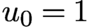 $u_0 = 1$
forward and backward over the ten trials.
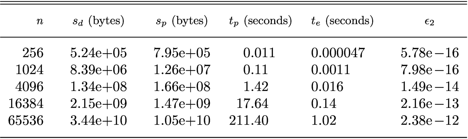
5 Ordinary differential equations
Orthogonal polynomials have been used in the numerical solution of ordinary differential equations for a long time, going back to Lanczos (Reference Lanczos1938). A key contribution was the integral reformulation method of Clenshaw (Reference Clenshaw1957), which observed that general linear differential equations with polynomial coefficients could be reduced to a banded, infinite-dimensional linear system using recurrence relationships of Chebyshev polynomials, via reformulation as an integral equation. Since then integral reformulation using Chebyshev polynomials has been rediscovered in a variety of contexts (Coutsias, Hagstrom and Torres Reference Coutsias, Hagstrom and Torres1996, Greengard Reference Greengard1991, Zebib Reference Zebib1984, Viswanath Reference Viswanath2015).
A related scheme from the finite element method (FEM) community is the p-FEM of Shen (Reference Shen1994), which uses a similar basis as Heinrichs (Reference Heinrichs1989) applied to the weak formulation. These approaches lead naturally to the p-FEM on tetrahedra of Beuchler and Schöberl (Reference Beuchler and Schöberl2006) and Li and Shen (Reference Li and Shen2010) discussed in Section 6.6. There are two major benefits of this approach due to it being applied to the weak formulation of a differential equation: (1) the discretizations are automatically symmetric if the differential equation is self-adjoint, and (2) only continuity (as opposed to continuity of the derivative) is required if an interval is subdivided into multiple elements (though this is less relevant for ODEs than for PDEs). However, p-FEMs are less versatile for higher-order equations and general boundary conditions, and they also require a problem to be posed in weak formulation before being discretized.
The idea of using recurrence relationships to represent differential operators using banded linear systems is a continuing theme in the ultraspherical spectral method of Olver and Townsend (Reference Olver and Townsend2013), where sparse recurrence relationships between ultraspherical polynomials are employed. The ultraspherical spectral method is similar in spirit to Clenshaw’s integral reformulation and p-FEMs, with the benefit of increased versatility. It automatically produces banded discretizations for general differential operators, including operators with both differentiation and multiplication, leading to optimal
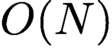 $O(N)$
complexity computations. In particular, it is applicable for Sturm–Liouville equations and high-order equations and is extensible to partial differential equations and singular integral equations, as discussed in Sections 6 and 7.
Each of the aforementioned methods produces a banded infinite-dimensional system which can be solved in multiple ways, as noted originally by Clenshaw (Reference Clenshaw1957):
The relations between the coefficients, obtained by application of the fundamental equations, constitute an infinite set of linear algebraic equations in the unknowns
 $a_r$
and
 $a_r^{(s)}$
, which can be solved to any required accuracy by recurrence or iteration. We shall usually use the former method …
In particular, there are various approaches.
-
(1) Shooting method. Guess the tail coefficients and do back-substitution (Clenshaw Reference Clenshaw1957).
-
(2) Finite section method. Truncate the operator and solve the resulting finite linear system.
-
(3)
$\tau $
-method. Perform a rectangular truncation that captures the operators exactly with extra columns added to make the problem square (Lanczos Reference Lanczos1938). -
(4) (F. W. J.) Olver’s algorithm. Perform adaptive Gaussian elimination until a convergence criterion is achieved, at which point perform back-substitution (Olver Reference Olver1967, Lozier Reference Lozier1980).
-
(5) Adaptive QR method. Perform adaptive Givens rotations or Householder reflections until a convergence criterion is achieved, at which point perform back-substitution (Olver and Townsend Reference Olver and Townsend2013).

A detailed description of the benefits and trade-offs of these techniques is outside the scope of this paper. Still, we will advocate for Olver’s algorithm for diagonally dominant discretizations and the adaptive QR algorithm otherwise, as they achieve adaptive error control and stability, which leads to faster algorithms as the same equation need not be solved multiple times.
Clenshaw’s integral reformulation, ultraspherical spectral methods and p-finite element methods are fast in the sense that they achieve
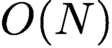 $O({N})$
complexity for N degrees of freedom, due to the sparsity of the discretization, provided any variable coefficients are smooth and therefore well-approximated by polynomials. There are a slew of non-fast methods based on collocation, Galerkin approximations and the Chebyshev-tau method that represent differentiation with a dense matrix. We will not discuss these methods further.
We also do not discuss in detail the convergence proofs of the various methods. For non-singular differential equations, Clenshaw’s integral reformulation, ultraspherical spectral methods and p-finite element methods represent them as operators that can be pre- or post-conditioned to be a compact perturbation of the identity. This gives us the machinery of second-kind Fredholm operators to rely on (Olver and Townsend Reference Olver and Townsend2013).
5.1 Clenshaw’s integral reformulation
The idea behind Chebyshev-based integral reformulation is to multiply the differential equation by indefinite integration operators on either the left or right and use the relationship given in Proposition A.17. Clenshaw (Reference Clenshaw1957) applied the relationship in Proposition A.17 on the right. For the Airy equation we find that
 $$ \begin{align*} u = {\mathcal{Q}}^2 \boldsymbol{T} \boldsymbol{v} = \boldsymbol{T} Q^2 \boldsymbol{v}, \end{align*} $$
where
 ${\mathcal {Q}}$
is the indefinite integration operator so that the zeroth Chebyshev coefficient is zero and
 $Q \equiv Q_T$
is the associated matrix from Proposition A.17.Footnote
6
For the Airy example we have
 $$ \begin{align*} ({\mathcal D}^2 - x) \iint \boldsymbol{T} \boldsymbol{v} = \boldsymbol{T} (I - X Q^2) \boldsymbol{v} = \boldsymbol{T} \boldsymbol{f}. \end{align*} $$
Cancelling out the (formally invertible) quasimatrix
 $\boldsymbol {T}$
we get an infinite-dimensional linear system:
 $$ \begin{align*} (I - X Q^2) \boldsymbol{v} = \boldsymbol{f}. \end{align*} $$
Note that this system is a compact perturbation of the identity, and so is readily solvable via, say, finite section.
A missing component so far is boundary conditions: we can find a particular solution using the above linear system, but not necessarily the solution we were after, and indeed with the standard Airy equation where
 $f = 0$
, we recover the rather uninteresting solution
 $\boldsymbol {v} = 0$
. Clenshaw, therefore, proposed a shooting method: initiate the recurrence from a large N using two different final conditions and iterate backwards, then combine with the constants of integration to match the prescribed boundary conditions.
In linear algebra terms, this is equivalent to appending additional unknowns corresponding to the low-order Chebyshev coefficients, and additional rows that impose the boundary conditions. That is, we write
 $$ \begin{align*} u(x) = (T_0 \mid T_1 \mid \boldsymbol{T} Q^2) \boldsymbol{v} {.} \end{align*} $$
So the Airy equation with boundary conditions becomes
 $$ \begin{align*} \begin{pmatrix} 1 & -1 & (1,-1,1,\ldots) Q^2 \\[2pt] 1 & 1 & (1,1,1,\ldots) Q^2 \\[2pt] -X_{:,0} & -X_{:,1} & I - X Q^2\end{pmatrix} \begin{pmatrix}c_0\\ c_1\\ \boldsymbol{v}\end{pmatrix} = \begin{pmatrix}a \\ b \\ \boldsymbol{f}\end{pmatrix}, \end{align*} $$
where
 $X_{:,j}$
is the jth column of the multiplication operator X.
Integral reformulation is straightforward to construct and leads to sparse, almost banded systems; see Figure 5.1 for the sparsity structure for the Airy equation (which is the same as the ultraspherical spectral method). This system can be efficiently solved, using either shooting techniques, as in Clenshaw (Reference Clenshaw1957), or linear algebra techniques such as adaptive QR of Olver and Townsend (Reference Olver and Townsend2013). It is generalizable to higher-order differential equations. However, it will not immediately work with Sturm–Liouville-type equations: in an operator like
 $ {\mathcal D} a(x) {\mathcal D} $
we cannot remove the leftmost derivative by multiplying on the right by integration operators without reformulating using integration by parts. Finally, it is not easily generalizable to higher-dimensional domains such as triangles.
A spy plot of the sparsity structure for Clenshaw’s integral reformulation and the ultraspherical spectral method (a) compared to the p-finite element method (b), for a
 $20 \times 20$
discretization for the Airy operator
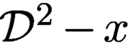 ${\mathcal D}^2 - x$
.
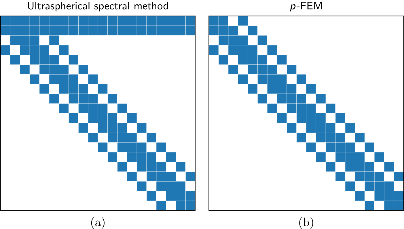
Remark 5.1. Note that Clenshaw did not truncate X and
 $Q^2$
and then multiply: because both are banded operators, it is possible to deduce the entries directly. We follow this approach: we have access to the true infinite-dimensional operators, which limits the source of errors.
5.2 Ultraspherical spectral method
The ultraspherical spectral method of Olver and Townsend (Reference Olver and Townsend2013) is an alternative approach for arriving at sparse discretizations, building on the observation that the domain and range of the equation need not be in the same basis. This gives more flexibility, and indeed enabled extensions to singular integral equations and partial differential equations outlined below.
We expand in Chebyshev basis
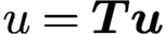 $u = \boldsymbol {T} \boldsymbol {u}$
. By changing continuous operators to discrete ones we arrive at
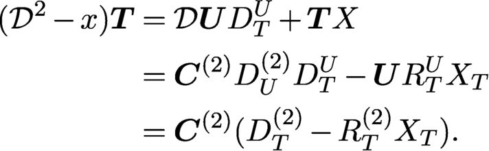 $$ \begin{align*} ({\mathcal D}^2 - x) \boldsymbol{T} & = {\mathcal D} \boldsymbol{U} D_T^U + \boldsymbol{T} X \\ & = \boldsymbol{C}^{(2)} D_U^{(2)} D_T^U - \boldsymbol{U} R_T^U X_T \\ & = \boldsymbol{C}^{(2)} (D_T^{(2)} - R_T^{(2)} X_T ). \end{align*} $$
Thus the Airy equation becomes
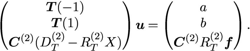 $$ \begin{align*} \begin{pmatrix}\boldsymbol{T}(-1) \\ \boldsymbol{T}(1) \\ \boldsymbol{C}^{(2)}(D_T^{(2)} - R_T^{(2)} X)\end{pmatrix} \boldsymbol{u} = \begin{pmatrix}a \\ b\\ \boldsymbol{C}^{(2)} R_T^{(2)} \boldsymbol{f}\end{pmatrix}. \end{align*} $$
We can then cancel out the (formally invertible) quasimatrix
 $\boldsymbol {C}^{(2)}$
to arrive at a discrete system:
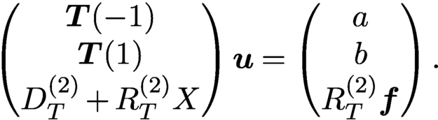 $$ \begin{align*} \begin{pmatrix}\boldsymbol{T}(-1) \\ \boldsymbol{T}(1) \\ D_T^{(2)} + R_T^{(2)} X\end{pmatrix} \boldsymbol{u} = \begin{pmatrix}a\\ b\\ R_T^{(2)} \boldsymbol{f}\end{pmatrix}. \end{align*} $$
Note that X is tridiagonal,
 $R_T^{(2)}$
has bandwidths
 $(0,4)$
and
 $D_T^{(2)}$
has bandwidths
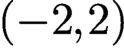 $(-2,2)$
, and as the product of banded matrices adds the bandwidths, the operator is banded with bandwidths
 $(1,5)$
. Thus the resulting system with the boundary is an almost banded linear system: it can be written as
 $$ \begin{align*} \text{{banded}} + \text{triu}(U V^{\top} ), \end{align*} $$
where
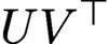 $U V^{\top }$
is a rank-2 matrix and the banded part has bandwidth
 $(3, 3)$
. A spy plot is shown in Figure 5.1. This structure is preserved under linear algebra operations such as Householder reflections, with the bandwidth of the banded part uniformly bounded. Thus it is amenable to fast linear algebra.
What makes the ultraspherical spectral method is its versatility. We can handle arbitrary functional constraints: Neumann conditions, Robin conditions, integral constraints, etc. For example, one can convert any linear ordinary differential operator with variable coefficients such as
 $$ \begin{align*} a_\nu(x) \displaystyle \frac{{\mathrm{d}}^\nu }{ {{\mathrm{d}}x}^\nu} + \cdots + a_2(x) \displaystyle \frac{{\mathrm{d}}^2 }{ {{\mathrm{d}}x}^2} + a_1(x) \displaystyle \frac{{\mathrm{d}} }{ {{\mathrm{d}}x}} + a_0(x) \end{align*} $$
to an (infinite) banded matrix,
 $$ \begin{align*} a_\nu(X_{(\nu)}) D_T^{(\nu)} + \cdots + R_{(2)}^{(\nu)} a_2(X_{(2)}) D_T^{(2)} + R_U^{(\nu)} a_1(X_U) D_T^U + R_T^{(\nu)}. \end{align*} $$
We do not require the equation to be given in reduced form: for example, a Sturm–Liouville operator
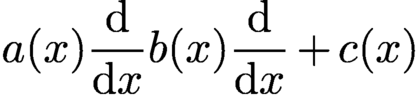 $$ \begin{align*} a(x) \displaystyle \frac{{\mathrm{d}} }{ {{\mathrm{d}}x}} b(x) \displaystyle \frac{{\mathrm{d}} }{ {{\mathrm{d}}x}} + c(x) \end{align*} $$
also leads to a banded matrix
 $$ \begin{align*} a(X_{(2)}) D_U^{(2)} b({X_{U}}) D_T^U + R_T^{(2)} c(X_T) \end{align*} $$
without having to use the product rule to simplify the differential equations. This is a fairly minor issue for second-order equations but can become significant for higher-order differential equations.
We can also handle general boundary conditions. For example, an arbitrary differential condition at a point
 $x_0$
of the form
 $$ \begin{align*} \beta_\mu u^{(\mu)}(x_0) + \cdots + \beta_1 u'(x_0) + \beta_0 u(x_0) \end{align*} $$
is represented by the row-vector
 $$ \begin{align*} \boldsymbol{C}^{(\mu)}(x_0) \bigl[\beta_\mu D_T^{(\mu)} + \cdots + \beta_1 R_U^{(\mu)} D_T^U + \beta_0 R_T^{(\mu)}\bigr] \end{align*} $$
and an integral constraint like
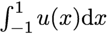 $\int _{-1}^1 u(x) {{\mathrm {d}}x}$
is represented by
 $$ \begin{align*} {(\boldsymbol{T}(1) - \boldsymbol{T}(-1)) Q_T.} \end{align*} $$
5.2.1 Example: Airy equation
As a simple example, we consider the Airy equation
 $$ \begin{align*} \epsilon^2 u^{\prime\prime} = x u \quad u(-1) = 1, u(1) = 0, \end{align*} $$
which is discretized as
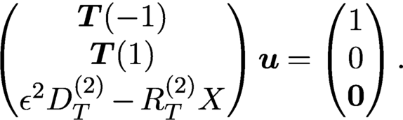 $$ \begin{align*} \begin{pmatrix}\boldsymbol{T}(-1) \\ \boldsymbol{T}(1) \\ \epsilon^2 D_T^{(2)} - R_T^{(2)} X\end{pmatrix} \boldsymbol{u} = \begin{pmatrix}1 \\ 0\\ \mathbf 0\end{pmatrix}. \end{align*} $$
In Figure 5.2(a) we plot the computed coefficients for four choices of
 $\epsilon $
, highlighting the need for fast algorithms. Note that the calculated coefficients converge well below machine precision. The fact that the tail is below machine precision is a consequence of the diagonal dominance of the discretization (it can be shown to converge in any space of algebraically decaying coefficients (Olver and Townsend Reference Olver and Townsend2013)). This makes the approach particularly appealing for adaptivity, as we can robustly choose the convergence criteria. Here we calculated the coefficients until they underflowed. In Figure 5.2(b) we show the timing for various
 $\epsilon $
using the adaptive criteria. This demonstrates the
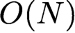 $O(N)$
complexity, as the N required to resolve the solution scales linearly with
 $\epsilon ^ {-1}$
.
The computed coefficients for the Airy equation (a) and the time taken to solve the Airy equation using the ultraspherical spectral methods with the adaptive QR method (b). The degrees of freedom needed to resolve the solution are proportional to
 $\epsilon ^{-1}$
.
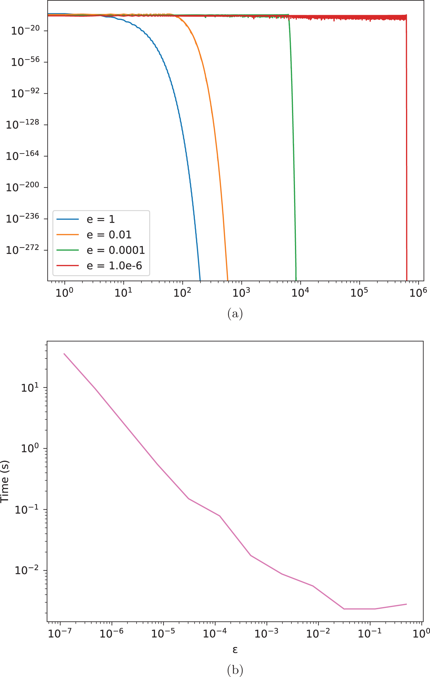
5.2.2 Example: catastrophes and integrals with coalescing saddles
Integrals with coalescing saddles arise in a number applications such as modelling tsunamis (Berry Reference Berry2007), and are defined by (Olver et al. Reference Olver, Lozier, Boisvert and Clark2010, 36.2.4)
 $$ \begin{align*} \Psi_K(\boldsymbol{x}) := \int_{-\infty}^\infty \exp{{\mathrm{i}} \Phi_K(t; \boldsymbol{x})} {{\mathrm{d}}t}, \quad \Phi_K(t; \boldsymbol{x}) := t^{K+2} + \sum_{m=1}^K x_m t^m. \end{align*} $$
We focus our discussion on
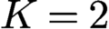 $K = 2$
, which is an integral due to Pearcey (Reference Pearcey1946), and given by
 $$ \begin{align*} \Psi(x,y) = \Psi_2(x, y) = \int_{-\infty}^\infty \exp{{\mathrm{i}} (t^4 + y t^2 + x t)} {{\mathrm{d}}t} . \end{align*} $$
Catastrophic integrals satisfy differential equations with respect to
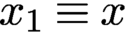 $x_1 \equiv x$
of order
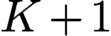 $K+1$
; in the case of the Pearcey integral we have (Olver et al. Reference Olver, Lozier, Boisvert and Clark2010, 32.10.4)
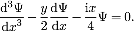 $$ \begin{align*} \displaystyle \frac{{\mathrm{d}}^3 \Psi }{ {{\mathrm{d}}x}^3} - \displaystyle \frac{y }{ 2} \displaystyle \frac{{\mathrm{d}} \Psi }{ {\mathrm{d}} x} - \displaystyle \frac{{\mathrm{i}} x }{ 4} \Psi = 0. \end{align*} $$
The ultraspherical spectral method gives a convenient way of discretizing this equation: if we write
 $$ \begin{align*} \Psi(x,y) = \boldsymbol{T}(x) \boldsymbol{u}(y) {,} \end{align*} $$
we have for each choice of y
 $$ \begin{align*} \biggl(D_T^{(3)} - \displaystyle \frac{y }{ 2} R_U^{(3)} D_T^U - \displaystyle \frac{{\mathrm{i}} }{ 4} R_T^{(3)} X_T\biggr) \boldsymbol{u}(y) = 0. \end{align*} $$
This is a third-order equation; however, we can evaluate
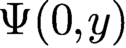 $\Psi (0,y)$
using a convergent series expansion (Olver et al. Reference Olver, Lozier, Boisvert and Clark2010, 36.8.1) and asymptotically accurate expansions for
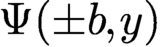 $\Psi (\pm b,y)$
where b is large, using Olver et al. (Reference Olver, Lozier, Boisvert and Clark2010, 36.11.2), thereby imposing three conditions. Thus each slice of y can be computed in
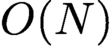 $O(N)$
operations. Putting everything together, we display the solution in Figure 5.3.
A depiction of the Pearcey integral, computed using the ultraspherical spectral method applied to a third-order differential equation in x for each y value.
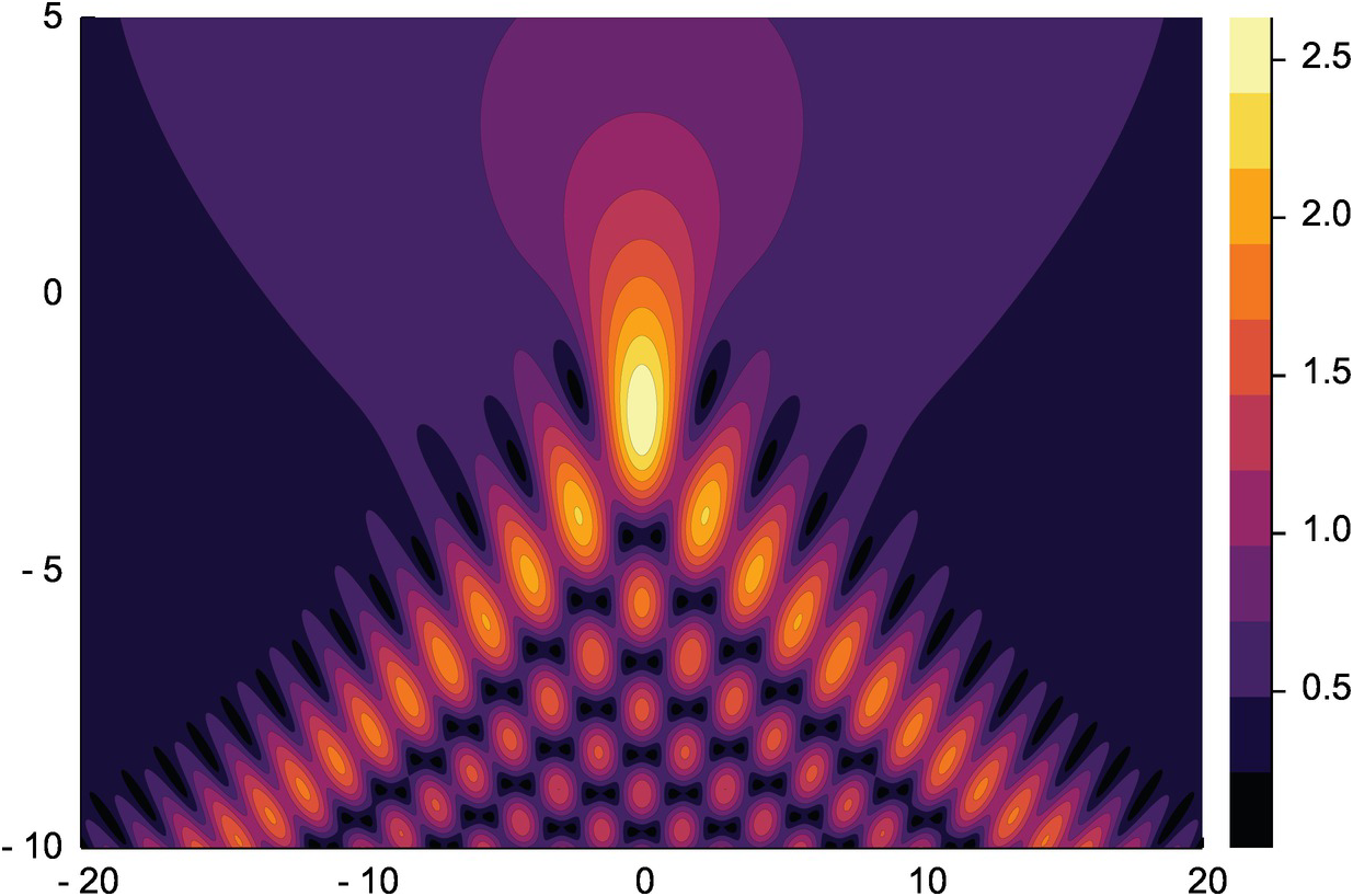
5.3 p-finite element methods
Finite element methods (FEM) have the attractive feature that they preserve self-adjointness of problems, and require only a weak formulation of a differential equation. The idea behind p-FEM as used by Beuchler and Schöberl (Reference Beuchler and Schöberl2006) is to use orthogonal polynomials to enable high polynomial order approximations for the test-and-trial space, maintaining sparsity in the process. This is readily explained in quasimatrix notation. Take for example the weak formulation of the Airy equation with Dirichlet conditions:
 $$ \begin{align*} -\langle v',u'\rangle - \langle v,x u\rangle = \langle v,f\rangle. \end{align*} $$
Write u and v in weighted Jacobi expansions and f in Legendre expansion:
 $$ \begin{align*} u = (1-x^2) \boldsymbol{C}^{(3/2)} \boldsymbol{u}, \quad v = (1-x^2) \boldsymbol{C}^{(3/2)} \boldsymbol{v}, \quad f = \boldsymbol{P} \boldsymbol{f}. \end{align*} $$
Then we have
 $$ \begin{align*} \langle v,x u\rangle & =\boldsymbol{v}^{\top} (\boldsymbol{C}^{(3/2)})^{\top} (1-x^2) x (1-x^2) \boldsymbol{C}^{(3/2)} \boldsymbol{u} \\ &= \boldsymbol{v}^{\top} (L_{(3/2)}^P)^{\top} \boldsymbol{P}^{\top} \boldsymbol{P} X_P L_{(3/2)}^P \boldsymbol{u} \end{align*} $$
and similarly
 $$ \begin{align*} \langle v',u'\rangle & =\boldsymbol{v}^{\top} ({\mathcal D} (1-x^2) \boldsymbol{C}^{(3/2)})^{\top} {\mathcal D} (1-x^2) \boldsymbol{C}^{(3/2)} \boldsymbol{u} \\ & = \boldsymbol{v}^{\top} (W_{(3/2)}^P)^{\top} \boldsymbol{P}^{\top} \boldsymbol{P} W_{(3/2)}^P \boldsymbol{u}. \end{align*} $$
Thus the differential equation becomes
 $$ \begin{align*} (- (W_{(3/2)}^P)^{\top} M_P W_{(3/2)}^P - ( L_{(3/2)}^P)^{(3/2)} M_P X_P L_{(3/2)}^P) \boldsymbol{u} = (L_{(3/2)}^P)^{\top} M \boldsymbol{f}, \end{align*} $$
where
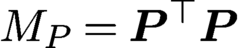 $M_P = \boldsymbol {P}^{\top } \boldsymbol {P}$
is the diagonal mass matrix.
The system is symmetric: since
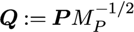 $\boldsymbol {Q} := \boldsymbol {P} M_P^{-1/2}$
are the orthonormalized Legendre polynomials, we have
 $$ \begin{align*} x \boldsymbol{P} M_P^{-1/2} = \boldsymbol{P} X_P M_P^{-1/2} = \boldsymbol{P} M_P^{-1/2} \tilde X = \boldsymbol{Q} \tilde X \end{align*} $$
so that
 $M_P X_P = M_P^{1/2} \tilde X M_P^{1/2}$
is symmetric. Thus square truncations are banded symmetric matrices. For positive definite problems we can therefore reliably use Cholesky decompositions, as implemented in LAPACK.
5.3.1 Example: a stochastic Airy equation
We consider a stochastic Airy equationFootnote 7 with Dirichlet conditions
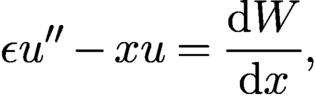 $$ \begin{align} \epsilon u^{\prime\prime} - x u = \displaystyle \frac{{\mathrm{d}} W }{ {\mathrm{d}} x}, \end{align} $$
where
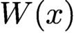 $W(x)$
is a Wiener process. The weak formulation of this equation is
 $$ \begin{align*} -\epsilon \langle v',u'\rangle - \langle v,x u\rangle = -\langle v', W\rangle, \end{align*} $$
which results in a banded discretization as above. This problem requires very large N to solve: as
 $\epsilon $
becomes small it becomes increasingly oscillatory, and we also need large N to approximate the Wiener process. We use the QR factorization (as opposed to the Cholesky factorization) as the Airy operator is not positive definite.
In Figure 5.4 we compute the solutions to this equation. We include the timings, which consist of (1) calculating the Legendre coefficients of W using transforms, (2) building the operator, (3) computing the QR factorization, and (4) solving the equation using the factorization. This results in a quasi-optimal complexity algorithm.
(a) Solutions to the stochastic Airy equation (5.1) with three choices of
 $\epsilon $
, computed using the p-FEM. (b) The timings in seconds for building, computing the QR factorization, and inverting using the pre-computed QR factorization.
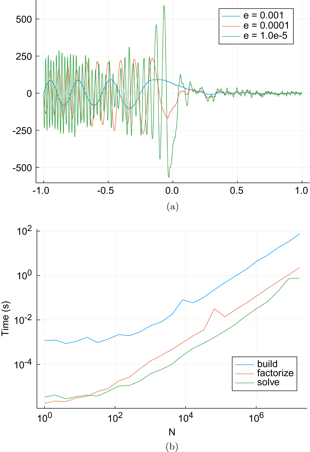
5.3.2 Example: beam equation
We now consider the clamped beam equation
 $$ \begin{align*} u_{tt} & = u_{xxxx},\\ u(0,x) & = u_0(x), u_t(0,x) = v_0(x), \\ u(t,-1) & = {u_x(t,-1) = u(t,1) = u_x(t,1) = 0}, \end{align*} $$
where we use the p-FEM to discretize in space. We solve the weak formulation
 $$ \begin{align*} \langle v, u_t\rangle = \langle \Delta v, \Delta u\rangle \end{align*} $$
using the space
 $u(t,x) =(1-x^2) \boldsymbol {P}^{(2,2)} \boldsymbol {u}(t)$
to arrive at the discretization
 $$ \begin{align*} \underbrace{(L_{(2,2)}^{(0,0)})\top M_P L_{(2,2)}^{(0,0)}}_M \boldsymbol{u}_t = \underbrace{(W_{(2,2)}^{(0,0)})^{\top} M_P W_{(2,2)}^{(0,0)}}_A \boldsymbol{u}. \end{align*} $$
This is a standard ODE with a mass matrix, where M is symmetric with bandwidths
 $(4,4)$
while A is diagonal.
In Figure 5.5 we demonstrate the solution of the beam equation. Since M and A are banded, we can perform implicit time-steps in
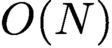 $O(N)$
operations, where we truncate the discretization to the first
 $N = 1000$
terms in x. We use the Rodas 5 time-stepping routine with time-step
 $0.01$
. As M is symmetric positive definite, we can use the banded Cholesky factorization.
A solution of the beam equation using the p-finite element method. We use
 $N = 1000$
spatial discretization with a time-step of
 $0.01$
with Rodas 5.
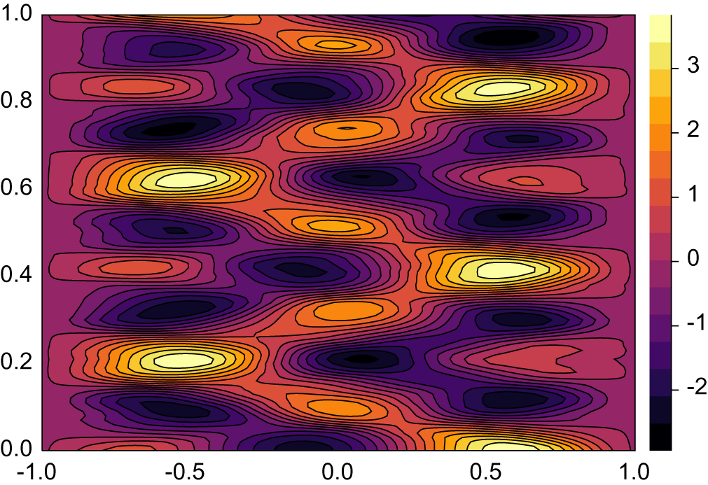
5.4 Domain decomposition
The p-finite element method naturally extends to multiple elements. For example, suppose we have a mesh
 $x_1 < x_2 < \cdots < x_M$
. Within each element we can use the bubble functions
 $$ \begin{align*} \begin{cases} (1-m_j(x)^2) \boldsymbol{C}^{(3/2)}(m_j(x)) & x_j \leq x \leq x_{j+1}, \\ 0 & \text{otherwise}, \end{cases} \end{align*} $$
where
 $m_j \colon [x_j,x_{j+1}] \rightarrow [-1,1]$
is the affine map. This is then combined with the low-order finite element basis
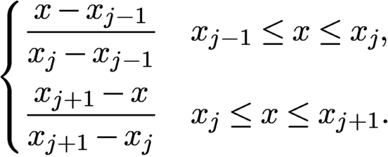 $$ \begin{align*} \begin{cases} \displaystyle \frac{x - x_{j-1} }{ x_j - x_{j-1}} & x_{j-1} \leq x \leq x_j, \\[10pt] \displaystyle \frac{x_{j+1} - x }{ x_{j+1} - x_{j}} & x_{j} \leq x \leq x_{j+1}. \end{cases} \end{align*} $$
As both the bubble functions and the additional low-order bases can both be transformed to piecewise Legendre polynomials, we can systematically deduce the resulting discretization using recurrence relationships. This discretization is extremely sparse, with low-rank communication between elements, due to the low-order terms. Interlacing the coefficients reduces this to a banded linear system whose bandwidth is dictated by the number of elements.
Ultraspherical spectral methods can also be incorporated into domain decomposition methods, where continuity conditions are enforced as boundary conditions. Alternatively, one may use integral reformulation, which Lee and Greengard (Reference Lee and Greengard1997) used to construct a very effective adaptive mesh refinement strategy.
5.5 Eigenvalue problems
The p-FEM and ultraspherical spectral method can be used to reduce differential eigenvalue problems to generalized eigenvalue problems. We demonstrate this on the Schrödinger equation:
 $$ \begin{align*} -u^{\prime\prime} + |x| u = \lambda u, \quad -20 < x < 20 \end{align*} $$
with Dirichlet conditions. The eigenstates are plotted in Figure 5.6. Since the potential is piecewise polynomial, the discretization is symmetric and banded, and the eigenvalues can be calculated in
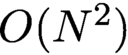 $O({N^2})$
complexity using a specialized solver (Schwarz Reference Schwarz1968, Crawford Reference Crawford1973, Kaufman Reference Kaufman1993, Kaufman Reference Kaufman2000). Here we decompose the interval into two elements.
The first 50 eigenstates of the Schrödinger equation with potential
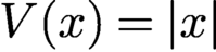 $V(x) = |x|$
computed using the p-FEM, with two elements.
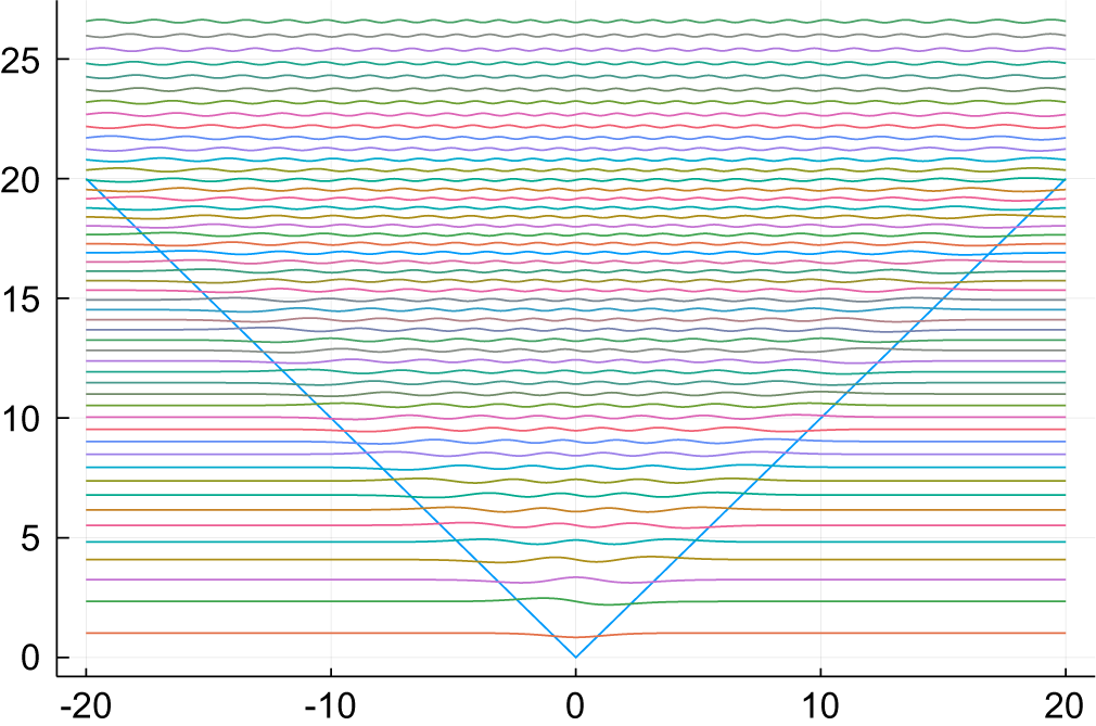
As an alternative to the Beucher–Schöberl p-FEM, Aurentz and Slevinsky (Reference Aurentz and Slevinsky2020) describe how basis recombination (Shen Reference Shen1994, Doha and Abd-Elhameed Reference Doha and Abd-Elhameed2002, Julien and Watson Reference Julien and Watson2009, Livermore Reference Livermore2010) can be leveraged to symmetrize the ultraspherical spectral method for self-adjoint problems while preserving the banded property that we have come to expect from spectral discretizations of linear problems. This method allows for more general self-adjoint boundary conditions, does not require the problem to be posed in the weak or self-adjoint form for the symmetry to transcend from problem to discretization, and may solve weakly defined problems by specifying relative discontinuity conditions in the basis.
In the self-adjoint setting, a
 $(2\nu )$
th-order linear differential eigenvalue problem with self-adjoint boundary conditions takes the form
 $$ \begin{align} & {\mathcal L} u = [(-{\mathcal D})^\nu({a}_\nu{\mathcal D}^\nu) + (-{\mathcal D})^{\nu-1}({a}_{\nu-1}{\mathcal D}^{\nu-1}) + \cdots + {a}_0 ]u = \lambda w u, \end{align} $$
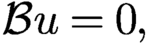 $$ \begin{align} & {\mathcal B} u = 0, \end{align} $$
where the usual conditions on the coefficients
 ${a}_i$
and w are required for a sensible solution; at the very least,
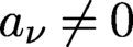 ${a}_\nu \ne 0$
, and
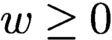 $w\ge 0$
and
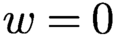 $w = 0$
only on a set of Lebesgue measure zero. In this form,
 ${\mathcal L}$
is a self-adjoint linear differential operator on a domain
 $D\subset {\mathbb R}$
in the Hilbert space
 $H = L^2(D,w(x){\mathrm \,d} x)$
provided it is accompanied by
 ${\mathcal B} \colon H \to {\mathbb C}^{2\nu }$
, a set of
 $2\nu $
self-adjoint boundary conditions. We will also assume that all the variable coefficients are at most degree-m polynomials, that is, for general smooth variable coefficients we initially approximate them by polynomials.
Given the quotient Hilbert space
 $H_{\mathcal B} := \{ u \in H \colon {\mathcal B} u = 0\}$
, a classical approach calls for a Ritz–Galerkin discretization for the trial and test functions taken from an n-dimensional subspace
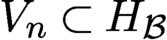 $V_n\subset H_{\mathcal B}$
. Indeed, when
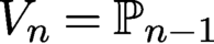 $V_n = \mathbb {P}_{n-1}$
and an orthonormal polynomial basis satisfying the boundary conditions is utilized, the discrete realization of
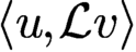 $\langle u, {\mathcal L} v\rangle $
is automatically symmetric (Hermitian). Unfortunately, the resulting discretizations are dense. Thus data-sparsity in problem formulations, such as (5.2) with finite-degree polynomial coefficients, is ignored when transformed into a computational problem, resulting in
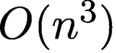 ${O} (n^3)$
complexity algorithms (Golub and Loan Reference Golub and Loan2013) for approximate eigenvalues and eigenfunctions.
Let
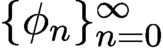 $\{\phi _n\}_{n=0}^\infty $
be an orthonormal polynomial basis for H with
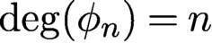 $\deg (\phi _n) = n$
. For linearly independent boundary conditions in
 ${\mathcal B}$
, let
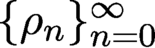 $\{\rho _n\}_{n=0}^\infty $
be the recombinations of the orthonormal basis
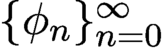 $\{\phi _n\}_{n=0}^\infty $
that annihilate
 ${\mathcal B}$
, guaranteeing
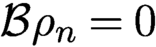 ${\mathcal B}\rho _n = 0$
. This assumption suggests the existence of an infinite-dimensional lower-triangular and banded conversion such that
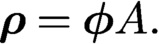 $$ \begin{align} \boldsymbol{\rho} = \boldsymbol{\phi} A. \end{align} $$
For a problem on
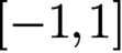 $[-1,1]$
with Dirichlet boundary conditions, the recombinations are the same basis used in Section 5.3, up to normalization. With the conversion in hand, a banded
 $QR$
factorization reveals the unitary operator mapping the orthonormal polynomial basis for H to the orthonormal polynomial basis
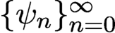 $\{\psi _n\}_{n=0}^\infty $
for the quotient Hilbert space
 $H_{\mathcal B}$
,
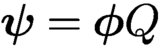 $\boldsymbol {\psi } = \boldsymbol {\phi } Q$
, and the auxiliary resulting conversion,
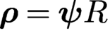 $\boldsymbol {\rho } = \boldsymbol {\psi } R$
. Finally, define the polynomials
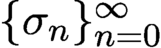 $\{\sigma _n\}_{n=0}^\infty $
by
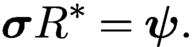 $$ \begin{align} \boldsymbol{\sigma}R^* = \boldsymbol{\psi}. \end{align} $$
Since we have
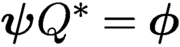 $\boldsymbol {\psi }Q^* = \boldsymbol {\phi }$
, we can gather all three adjoint conversions together to obtain
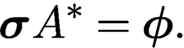 $$ \begin{align} \boldsymbol{\sigma}A^* = \boldsymbol{\phi}. \end{align} $$
Aurentz and Slevinsky (Reference Aurentz and Slevinsky2020) used these four bases to prove that the Petrov–Galerkin scheme for (5.2) is symmetric definite and banded, where the solution is formally represented by
 $u(x) = \boldsymbol {\rho } \boldsymbol {v} = \boldsymbol {\psi } R\boldsymbol {v} = \boldsymbol {\psi } \boldsymbol {u} = \boldsymbol {\phi } A\boldsymbol {v} = \boldsymbol {\phi } \boldsymbol {w}$
and the residuals are estimated by
 $\boldsymbol {\sigma }$
.
5.5.1 The Petrov–Galerkin scheme is self-adjoint
It follows by classical arguments that the Ritz–Galerkin scheme is self-adjoint:
 $$ \begin{align*} {\mathcal L} \boldsymbol{\psi} \boldsymbol{u} = \boldsymbol{\psi} L\boldsymbol{u} = \lambda w\boldsymbol{\psi} \boldsymbol{u} = \lambda \boldsymbol{\psi} M\boldsymbol{u}, \end{align*} $$
where
 $L = L^*\in {\mathbb C}^{\infty \times \infty }$
and
 $M = M^*\in {\mathbb C}^{\infty \times \infty }$
is positive definite. If we use
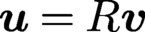 $\boldsymbol {u} = R\boldsymbol {v}$
and (5.5) to represent
 $\boldsymbol {\psi }$
in terms of
 $\boldsymbol {\sigma }$
, the symmetry may be imported into the Petrov–Galerkin scheme
 $$ \begin{align*} \boldsymbol{\sigma} R^*LR \boldsymbol{v} = \lambda \boldsymbol{\sigma} R^*MR\boldsymbol{v}. \end{align*} $$
Both
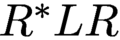 $R^*LR$
and
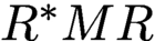 $R^*MR$
are self-adjoint and the latter is also positive definite.
5.5.2 The Petrov–Galerkin scheme is banded
Considering the Petrov–Galerkin scheme
 $$ \begin{align*} {\mathcal L} \boldsymbol{\rho} \boldsymbol{v} = \lambda w \boldsymbol{\rho} \boldsymbol{v}, \end{align*} $$
the combination of (5.4) and (5.6) informs us that
 $w\boldsymbol {\rho } = w\boldsymbol {\phi } A = \boldsymbol {\phi } M_B A = \boldsymbol {\sigma } A^*M_B A$
, where
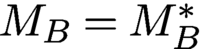 $M_B = M_B^*$
is also positive definite and banded by executing the Clenshaw–Smith algorithm with the orthonormal polynomials’ Jacobi operator. Similarly,
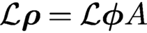 ${\mathcal L} \boldsymbol {\rho } = {\mathcal L} \boldsymbol {\phi } A$
, and by the ultraspherical spectral method (Olver and Townsend Reference Olver and Townsend2013), there exists a banded discretization of
 ${\mathcal L}$
, namely
 $L_B$
, mapping normalized Legendre polynomials to normalized Jacobi polynomials with integer parameters in proportion to the highest derivatives. Applying the inverse banded conversion operator, and further utilizing
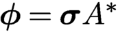 $\boldsymbol {\phi } = \boldsymbol {\sigma } A^*$
, we arrive at
 $$ \begin{align} \boldsymbol{\sigma} A^* C^{-1} L_B A \boldsymbol{v} = \lambda \boldsymbol{\sigma} A^*M_BA\boldsymbol{v}. \end{align} $$
At first glance, this formula does not appear to guarantee a banded discretization, due to the appearance of the inverse of a banded matrix. To show that the discretization is indeed banded, we note that the conversion matrix C is upper-triangular and banded, which means that its inverse will not extend the bandwidth of
 $L_BA$
any lower. Since
 $A^*$
is also upper-triangular and since the Petrov–Galerkin scheme is self-adjoint, we conclude that it must be banded above as well.
5.5.3 A sixth-order generalized eigenvalue problem
Aurentz and Slevinsky (Reference Aurentz and Slevinsky2020) show through several numerical and theoretical applications that the method is general, versatile and easy to use. They show that piecewise defined problems on bounded and unbounded domains may be stitched together with continuity conditions. They also show that the method applies to higher-order problems with ease.
The following sixth-order generalized eigenvalue problem of Gutierrez and Laura (Reference Gutierrez and Laura1995) models the vibration of non-uniform rings:
 $$ \begin{align} & \{(-{\mathcal D})^3 [g{\mathcal D}^3] - (-{\mathcal D})^2 [2\pi^2g{\mathcal D}^2] + (-{\mathcal D})[(\pi^4g+\pi^2g^{\prime\prime}){\mathcal D}]\} u\nonumber\\ & \quad = \lambda\{(-{\mathcal D})[\pi^4f{\mathcal D}] + \pi^6 f\}u, \end{align} $$
where
 $f(x) = 1+4(1-r)[(x-{1}/{2})^2-{1}/{4}]$
,
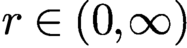 $r\in (0,\infty )$
is a thickness parameter,
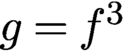 $g = f^3$
, and the boundary conditions are
 $u = u' = u^{\prime \prime \prime } = 0$
at both
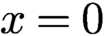 $x=0$
and
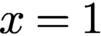 $x=1$
. Due to the third-order derivatives in the boundary conditions, they may not be implemented by multiplying an orthogonal polynomial expansion by a polynomial weight, and thus require basis recombination.
With sixth-order derivatives in the first operator in (5.8), this is by all accounts an ill-conditioned generalized eigenvalue problem. And as
 $r\rightarrow 0$
, this ill-conditioning is compounded by the fact that both linear operators become singular as the smallest generalized eigenvalue tends to zero.
Using the general Rayleigh quotient iteration (Rayleigh Reference Rayleigh1937, Parlett Reference Parlett1974) in
 $256$
-bit extended precision, the first four computed eigenvalues are tabulated in Table 5.1. Figure 5.7 tracks the first ten eigenvalues as
 $r\rightarrow 0$
.
The first four computed eigenvalues of (5.8) with
 $r=1$
in
 $256$
-bit extended precision, computed using the method of Aurentz and Slevinsky (Reference Aurentz and Slevinsky2020) and rounded to fit this page.
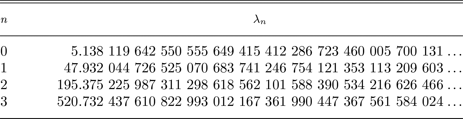
The first ten generalized eigenvalues of (5.8) as functions of the thickness parameter r. Figure reproduced from Aurentz and Slevinsky (Reference Aurentz and Slevinsky2020) with permission. Copyright © 2020 Elsevier.
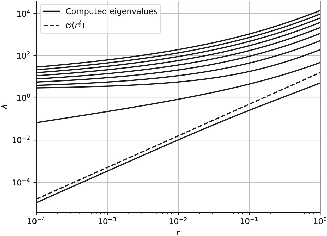
6 Partial differential equations
Multivariate OPs on rectangles/hypercubes and triangles/tetrahedra have played a central role in spectral element methods for partial differential equations. For triangles, see Dubiner (Reference Dubiner1991) and Karniadakis and Sherwin (Reference Karniadakis and Sherwin2013) for a comprehensive overview. These methods result in dense matrices for large p.
Recently, approaches for sparse discretizations for large p have been introduced in the p-finite element method on triangles (Beuchler and Schöberl Reference Beuchler and Schöberl2006, Li and Shen Reference Li and Shen2010) and the ultraspherical spectral method on rectangles (Townsend and Olver Reference Townsend and Olver2015), disks (Vasil et al. Reference Vasil, Burns, Lecoanet, Olver, Brown and Oishi2016) and triangles (Olver et al. Reference Olver, Townsend and Vasil2019).
Our model problem is the multivariate analogue of the Airy equation: a variable coefficient inhomogeneous Helmholtz equation
 $$ \begin{align*} \Delta u + k^2 x y^2 u = f(x,y) {.} \end{align*} $$
We will consider both squares and triangles in two dimensions. The type of boundary conditions allowed depends on the method under discussion.
6.1 Ultraspherical spectral methods on rectangles
On rectangular domains it is natural to use tensor product bases, and thus we consider the expansion of the form
 $$ \begin{align*} u(x,y) = \boldsymbol{T}^2(x,y) U = \boldsymbol{T}(x) U \boldsymbol{T}(y)^{\top} , \end{align*} $$
where U is an infinite matrix of coefficients and
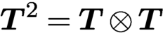 $\boldsymbol {T}^2 = \boldsymbol {T} \otimes \boldsymbol {T}$
. The separable nature of the decomposition makes it straightforward to construct partial differential operators from ordinary differential operators, for example
 $$ \begin{align*} \displaystyle \frac{\partial u }{ \partial x} = \boldsymbol{U}(x) D_T^U U \boldsymbol{T}(y)^{\top} = (\boldsymbol{U} \otimes \boldsymbol{T})(x,y) (D_T^U \otimes I) U. \end{align*} $$
Thus we can immediately construct the partial derivatives
 $$ \begin{align*} {\partial_x^2} \boldsymbol{T}^2 & = (\boldsymbol{C}^{(2)} D_T^{(2)} ) \otimes \boldsymbol{T} = (\boldsymbol{C}^{(2)} \otimes \boldsymbol{T}) (D_T^{(2)} \otimes I) = \boldsymbol{C}^{(2,2)} (D_T^{(2)} \otimes R_T^{(2)}) {,}\\ {\partial_y^2} \boldsymbol{T}^2 & = (\boldsymbol{T} \otimes \boldsymbol{C}^{(2)}) (I \otimes D_T^{(2)}) = \boldsymbol{C}^{(2,2)}(R_T^{(2)} \otimes D_T^{(2)}), \end{align*} $$
where
 $\boldsymbol {C}^{(a,b)} = \boldsymbol {C}^{(a)} \otimes \boldsymbol {C}^{(b)}$
. Thus we have
 $$ \begin{align*} \Delta \boldsymbol{T}^2 = \boldsymbol{C}^{(2,2)} \underbrace{[ D_T^{(2)} \otimes R_T^{(2)} + R_T^{(2)} \otimes D_T^{(2)}]}_{\Delta_{T,T}^{(2,2)}}. \end{align*} $$
Similarly, we have
 $$ \begin{align*} x \boldsymbol{T} = \boldsymbol{C}^{(2,2)} \underbrace{[ (R_T^{(2)} X_T ) \otimes I]}_{X} {\quad\text{and}\quad} y \boldsymbol{T} = \boldsymbol{C}^{(2,2)} \underbrace{[I \otimes (R_T^{(2)} X_T ) ]}_{Y}. \end{align*} $$
Putting everything together, we have
 $$ \begin{align*} [\Delta + x y^2] \boldsymbol{T}^2 = \boldsymbol{C}^{(2,2)} \bigl[ \Delta_{T,T}^{(2,2)} + R_{T,T}^{(2,2)} X Y^2\bigr], \end{align*} $$
where
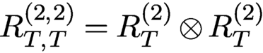 $R_{T,T}^{(2,2)} = R_T^{(2)} \otimes R_T^{(2)}$
. This is a sparse discretization.
We can similarly specify boundary conditions which are particularly nice for separable boundary conditions. For example, a Neumann condition on the top of an interval can be written as
 $$ \begin{align*} u_y(x,1) = (\boldsymbol{T} \otimes \boldsymbol{U}(1)) (I \otimes D_T^U) U = \boldsymbol{T}(x) U (D_T^U)^{\top} \boldsymbol{U}(1)^{\top}. \end{align*} $$
Putting everything together, if we write the right-hand side as
 $$ \begin{align*} f(x,y) = \boldsymbol{C}^{(2,2)} F \end{align*} $$
and the boundary data given in Chebyshev expansions as
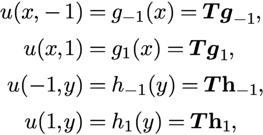 $$ \begin{align*} u(x,-1) & = g_{-1}(x) = \boldsymbol{T} \boldsymbol{g}_{-1}, \\[2pt] u(x,1) & = g_{1}(x) = \boldsymbol{T} \boldsymbol{g}_{1}, \\[2pt] u(-1,y) & = h_{-1}(y) = \boldsymbol{T} \mathbf h_{-1}, \\[2pt] {u(1, y)} &= {h_1(y) = \boldsymbol{T} \mathbf h_1,} \end{align*} $$
then we can express the variable coefficient Helmholtz problem with Dirichlet conditions as
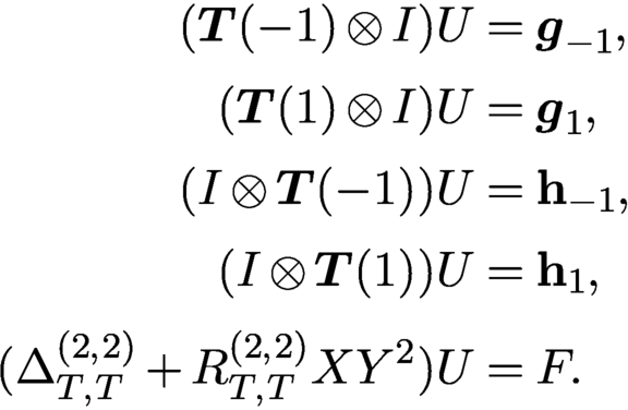 $$ \begin{align*} (\boldsymbol{T}(-1) \otimes I) U & = \boldsymbol{g}_{-1}, \\[2pt] (\boldsymbol{T}(1) \otimes I) U & = \boldsymbol{g}_{1}, \\[2pt] (I \otimes \boldsymbol{T}(-1)) U & = \mathbf h_{-1}, \\[2pt] (I \otimes \boldsymbol{T}(1)) U & = \mathbf h_{1}, \\[2pt] (\Delta_{T,T}^{(2,2)} +R_{T,T}^{(2,2)} X Y^2) U & = F. \end{align*} $$
Alternatively, we can view this as the following matrix problem:
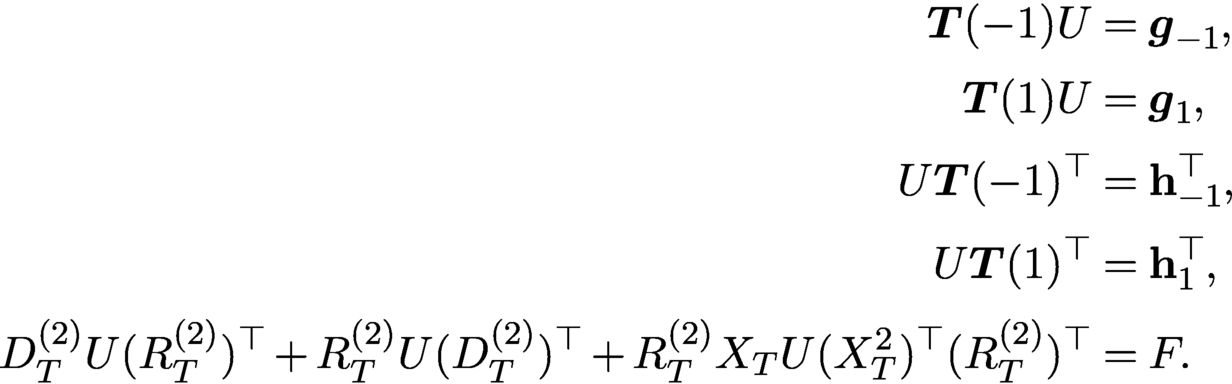 $$ \begin{align*} \boldsymbol{T}(-1) U & = \boldsymbol{g}_{-1}, \\[2pt] \boldsymbol{T}(1) U & = \boldsymbol{g}_{1}, \\[2pt] U\boldsymbol{T}(-1)^{\top} & = \mathbf h_{-1}^{\top}, \\[2pt] U\boldsymbol{T}(1)^{\top} & = \mathbf h_{1}^{\top}, \\[2pt] D_T^{(2)} U (R_T^{(2)})^{\top} + R_T^{(2)} U (D_T^{(2)})^{\top} + R_T^{(2)} X_T U (X_T^2)^{\top} (R_T^{(2)})^{\top} & = F. \end{align*} $$
This can be converted into a sparse linear system by choosing an ordering for the coefficients of U.
6.2 Sylvester equations
Townsend and Olver (Reference Townsend and Olver2015) observed that the boundary conditions in the matrix formulation of the problem can be used to eliminate degrees of freedom in the differential equation, thereby reducing the equation to a generalized Sylvester equation, that is, we wish to solve an equation of the form
 $$ \begin{align*} A_1 U B_1^{\top} + \cdots + A_r U B_r^{\top} = F, \end{align*} $$
where all
 $A_j$
and
 $B_j$
are sparse matrices, and r is known as the separability rank of the partial differential operator. For the special case of
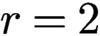 $r = 2$
this can be accomplished using a Schur factorization: find Q and Z orthogonal so that
 $A_1 = Q R_1 Z$
and
 $A_2 = Q R_2 Z$
, thus reducing the problem to
 $$ \begin{align*} R_1 V B_1^{\top} + R_2 V B_2^{\top} = Q^{\top} F \end{align*} $$
so that
 $V = Z U$
. This can be solved via back-substitutions as a sequence of sparse linear solves in
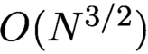 $O({N^{3/2}})$
complexity for N degrees of freedom.
As an example, consider the ‘good’ Helmholtz equation with Neumann conditions:
 $$ \begin{align*} \Delta u - k^2 u = 0, \quad u_x(\pm 1,y) =u_y(x,\pm 1) = 1. \end{align*} $$
We can write this in rank-2 form as
 $$ \begin{align*} (D_T^{(2)} - k^2 S_T^{(2)}) U (S_T^{(2)})^{\top} + S_T^{(2)} U (D_T^{(2)})^{\top} = 0. \end{align*} $$
The solution appears in Figure 6.1.
The solution to the screened Poisson equation using the ultraspherical spectral method.
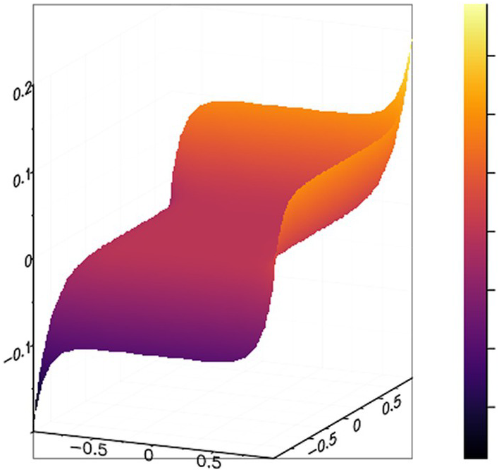
6.3 Fast Poisson solvers
In the particular situation of Poisson’s equation with zero homogeneous Dirichlet conditions, that is,
 $$ \begin{align} u_{xx} + u_{yy} = f, \quad (x,y)\in[-1,1]^2, \quad u(\pm1,\cdot) = u(\cdot,\pm 1) = 0{,} \end{align} $$
Fortunato and Townsend (Reference Fortunato and Townsend2019) take the idea a step further and develop an
 $O({N\log N \log (1/\epsilon )})$
complexity solver. First, it is noted that since (6.1) has homogeneous Dirichlet conditions, the solution can be written as
 $u(x,y) = (1-x^2)(1-y^2)v(x,y)$
for some function
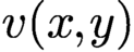 $v(x,y)$
. So the function
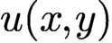 $u(x,y)$
is expanded in a carefully selected ultraspherical polynomial basis
 $$ \begin{align} u(x,y) = (1-x^2) \boldsymbol{\tilde C}^{(3/2)}(x) U \boldsymbol{\tilde C}^{(3/2)}(y)^{\top} (1-y^2){,}\quad (x,y)\in[-1,1]^2{,} \end{align} $$
where
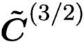 $ \boldsymbol {\tilde C}^{(3/2)}$
are the orthonormalized ultraspherical polynomials. These OPs are selected because
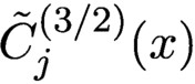 $\smash {\tilde {C}^{(3/2)}_j(x)}$
is an eigenfunction of the differential operator
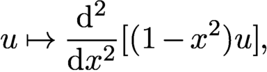 $$ \begin{align*} \smash{u\mapsto\displaystyle \frac{{\mathrm{d}}^2}{{\mathrm{d}} x^2} [(1-x^2)u]}, \end{align*} $$
that is,
 $$ \begin{align*} {\mathcal D}^2 [(1-x^2)\boldsymbol{\tilde{C}}^{(3/2)}] = \boldsymbol{\tilde{C}}^{(3/2)} \underbrace{\operatorname{diag}{(- (j+1)(j+2))}_{j=0,1,\ldots}}_\Lambda. \end{align*} $$
This means that (6.1) can be discretized as a generalized Sylvester matrix equation of the form
 $$ \begin{align} \Lambda U (I - \tilde X_{(3/2)}^2) + (I - \tilde X_{(3/2)}^2) U \Lambda^{\top} = F, \end{align} $$
where U is the matrix of expansion coefficients in (6.2), F is the matrix of bivariate
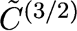 $\tilde {C}^{(3/2)}$
expansion coefficients for f, that is,
 $$ \begin{align*} f(x,y) = \boldsymbol{\tilde C}^{(3/2)}(x) F \boldsymbol{\tilde C}^{(3/2)}(y)^{\top}, \end{align*} $$
and
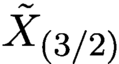 $\tilde X_{(3/2)}$
is the
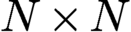 $N\times N$
matrix that represents multiplication by
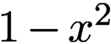 $1-x^2$
in the
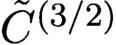 $\tilde {C}^{(3/2)}$
basis (which is symmetric). The Sylvester equation in (6.3) is rearranged and solved by an alternating direction implicit method (Fortunato and Townsend Reference Fortunato and Townsend2019).
6.4 Ultraspherical spectral methods on disks
There are fundamentally two approaches to spectral methods on disks: treat them as separable geometries using polar coordinates, or use non-separable bases. It is possible to construct ultraspherical spectral methods using either approach, with various trade-offs between the techniques. For separable techniques, see Wilber, Townsend and Wright (Reference Wilber, Townsend and Wright2017). Figure 6.2 repeats a simulation from Torres and Coutsias (Reference Torres and Coutsias1999) showing the successful use of spectral methods in solving Navier–Stokes in a disk.
Navier–Stokes simulation using spectral methods at time slices
 $t = 0,30,60,90,120,150$
.
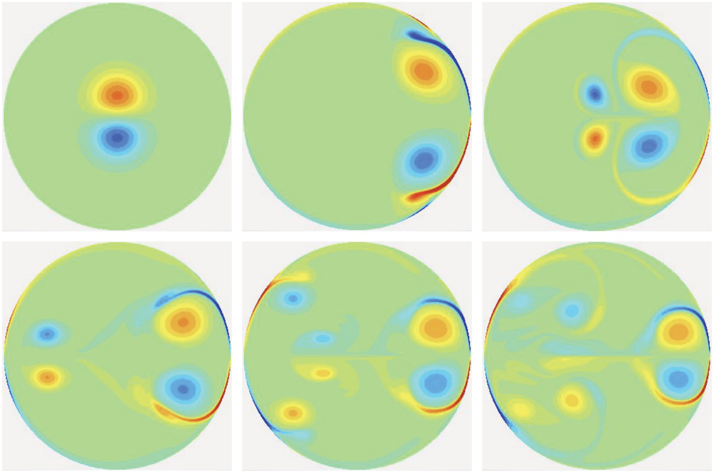
Alternatively, we can use orthogonal polynomials on a disk as in Vasil et al. (Reference Vasil, Burns, Lecoanet, Olver, Brown and Oishi2016), using generalized Zernike polynomials, which have the benefit of not having any (weak) singularities at the origin: they are polynomials in Cartesian coordinates x and y. Consider a function decomposed into Fourier modes, that is,
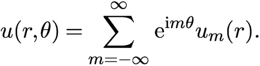 $$ \begin{align*} u(r,\theta) = \sum_{m = -\infty}^\infty \,{\mathrm{e}}^{{\mathrm{i}} m \theta}u_m(r). \end{align*} $$
We define two linear operators
 ${\mathcal D}_\pm $
via their action on each Fourier mode:
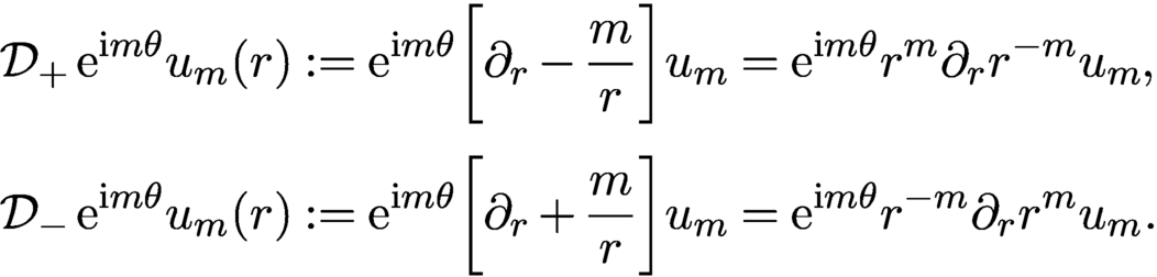 $$ \begin{align*} \begin{aligned} {\mathcal D}_+ \,{\mathrm{e}}^{{\mathrm{i}} m \theta} u_m(r) & := {\mathrm{e}}^{{\mathrm{i}} m \theta} \biggl[\partial_r - \displaystyle \frac{m}{ r} \biggr] u_m = {\mathrm{e}}^{{\mathrm{i}} m \theta} r^m \partial_r r^{-m} u_m, \\[3pt] {\mathcal D}_- \,{\mathrm{e}}^{{\mathrm{i}} m \theta} u_m(r) & := {\mathrm{e}}^{{\mathrm{i}} m \theta} \biggl[\partial_r + \displaystyle \frac{m}{ r} \biggr] u_m = {\mathrm{e}}^{{\mathrm{i}} m \theta} r^{-m} \partial_r r^{m} u_m. \end{aligned} \end{align*} $$
For the generalized Zernike polynomials these operators are diagonal with an appropriate change of basis, and hence can be combined to construct the Laplacian and other differential operators arising in applications. Fast transforms between Zernike polynomials and tensor product bases exist (Slevinsky Reference Slevinsky and Olver2017).
6.5 Ultraspherical spectral methods on triangles
Olver et al. (Reference Olver, Townsend and Vasil2019) introduced the ultraspherical spectral method using orthogonal polynomials on the triangle. As in the disk, we no longer have a tensor product structure without a change of coordinates, but the sparsity of discretizations is preserved. For Jacobi polynomials on the triangle
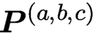 $\boldsymbol {P}^{(a,b,c)}$
there exist sparse matrices
 $$ \begin{align*} D_{x,(a,b,c)}^{(a+1,b,c+1)}\quad\text{and}\quad D_{y,(a,b,c)}^{(a,b+1,c+1)} \end{align*} $$
satisfying (Corollary B.2)
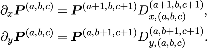 $$ \begin{align*} {\partial_x} \boldsymbol{P}^{(a,b,c)} & = \boldsymbol{P}^{(a+1,b,c+1)} D_{x,(a,b,c)}^{(a+1,b,c+1)}, \\ {\partial_y} \boldsymbol{P}^{(a,b,c)} & = \boldsymbol{P}^{(a,b+1,c+1)} D_{y,(a,b,c)}^{(a,b+1,c+1)}. \end{align*} $$
Likewise, we have sparse conversion matrices satisfying
 $$ \begin{align*} \boldsymbol{P}^{(a,b,c)} = \boldsymbol{P}^{(a+i,b+j,c+k)} R_{(a,b,c)}^{(a+i,b+j,c+k)}{,} \end{align*} $$
for any integers
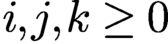 $i,j,k \geq 0$
. We can therefore compose these to construct sparse partial derivatives of the form
 $$ \begin{align*} {\partial_x} \boldsymbol{P}^{(a,b,c)} = \boldsymbol{P}^{(a+i+1,b+j,c+k+1)} \underbrace{R_{(a+1,b,c+1)}^{(a+i+1,b+j,c+k+1)} D_{x,(a,b,c)}^{(a+1,b,c+1)}}_{D_{x,(a,b,c)}^{(a+i+1,b+j,c+k+1)}}. \end{align*} $$
In particular, we can construct a sparse representation of the Laplacian via
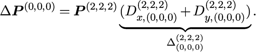 $$ \begin{align*} \Delta \boldsymbol{P}^{(0,0,0)} = \boldsymbol{P}^{(2,2,2)} \underbrace{(D_{x,(0,0,0)}^{(2,2,2)} + D_{y,(0,0,0)}^{(2,2,2)})}_{\Delta_{(0,0,0)}^{(2,2,2)}}. \end{align*} $$
The sparsity structure is depicted in Figure 6.3(a).
The sparsity pattern of the Laplacian
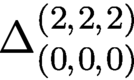 $\Delta _{(0,0,0)}^{(2,2,2)}$
(a), the weighted Laplacian
 $\Delta _W$
(b) and the weighted variable coefficient Helmholtz operator
 $\Delta _W + S_{(0,0,0)}^{(1,1,1)} v(X, Y) L_{(1,1,1)}^{(0,0,0)}$
with
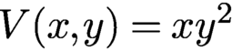 $V(x,y) = x y^2$
(c). The weak Laplacian in p-FEM has the same sparsity structure as (b) and (c), with the added benefit of symmetry in the coefficients. Figure reproduced from Olver et al. (Reference Olver, Townsend and Vasil2019) with permission. Copyright © 2019 Society for Industrial and Applied Mathematics. All rights reserved.
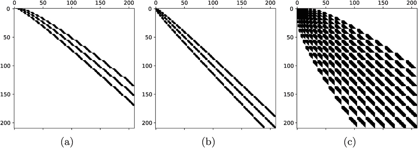
6.5.1 Dirichlet boundary conditions
Boundary conditions are more complicated, so let us consider the case of zero Dirichlet conditions by incorporating it into the basis. That is, we use the bubble functions
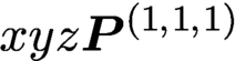 $x y z \boldsymbol {P}^{(1,1,1)}$
, where
 $z := 1-x-y$
as in the p-FEM discussed below. Using the weighted differentiation recurrences (Corollary B.3), we arrive at
 $$ \begin{align*} \Delta x y z \boldsymbol{P}^{(1,1,1)} = \boldsymbol{P}^{(1,1,1)} \underbrace{(D_{x,(0,0,0)}^{(1,1,1)} W_{x,(1,1,1)}^{(0,0,0)} + D_{y,(0,0,0)}^{(1,1,1)} W_{y,(1,1,1)}^{(0,0,0)})}_{\Delta_W}. \end{align*} $$
Thus we arrive at a discretization of the variable coefficient Helmholtz equation:
 $$ \begin{align*} ( \Delta_{W} + R_{(0,0,0)}^{(1,1,1)} X Y^2 L_{(1,1,1)}^{(0,0,0)}) \boldsymbol{u} = \boldsymbol{f}, \end{align*} $$
where
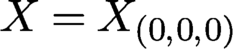 $X = X_{(0,0,0)}$
,
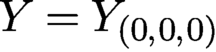 $Y = Y_{(0,0,0)}$
and
 $$ \begin{align*} f(x,y) = \boldsymbol{P}^{(1,1,1)}(x,y) \boldsymbol{f}. \end{align*} $$
The sparsity structure of
 $\Delta _W$
and the variable coefficient Helmholtz equation is depicted in Figure 6.3(a).
To handle non-zero Dirichlet conditions we use the basis
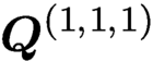 $\boldsymbol {Q}^{(1,1,1)}$
defined in Appendix B.2, which supplement
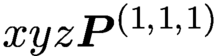 $x y z \boldsymbol {P}^{(1,1,1)}$
to include the missing polynomials. We have weighted partial derivatives
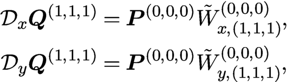 $$ \begin{align*} \begin{aligned} {\mathcal D}_x \boldsymbol{Q}^{(1,1,1)} & = \boldsymbol{P}^{(0,0,0)} \tilde W_{x,(1,1,1)}^{(0,0,0)}, \\ {\mathcal D}_y \boldsymbol{Q}^{(1,1,1)} & = \boldsymbol{P}^{(0,0,0)} \tilde W_{y,(1,1,1)}^{(0,0,0)}{,} \end{aligned} \end{align*} $$
and thus we have
 $$ \begin{align*} \Delta \boldsymbol{Q}^{(1,1,1)} = \boldsymbol{P}^{(1,1,1)} \underbrace{(D_{x,(0,0,0)}^{(1,1,1)} \tilde W_{x,(1,1,1)}^{(0,0,0)} + D_{y,(0,0,0)}^{(1,1,1)} \tilde W_{y,(1,1,1)}^{(0,0,0)})}_{\Delta_{\tilde W}}. \end{align*} $$
The basis also has a sparse block-banded restriction to a Legendre expansion along each edge (Proposition B.9) and is given by
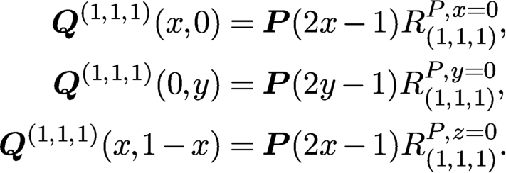 $$ \begin{align*} \boldsymbol{Q}^{(1,1,1)}(x,0) & = \boldsymbol{P}(2x-1) R_{(1,1,1)}^{P,x=0}, \\ \boldsymbol{Q}^{(1,1,1)}(0,y) & = \boldsymbol{P}(2y-1) R_{(1,1,1)}^{P,y=0}, \\ \boldsymbol{Q}^{(1,1,1)}(x,1-x) & = \boldsymbol{P}(2x-1) R_{(1,1,1)}^{P,z=0}. \end{align*} $$
Thus we arrive at the following discretization:
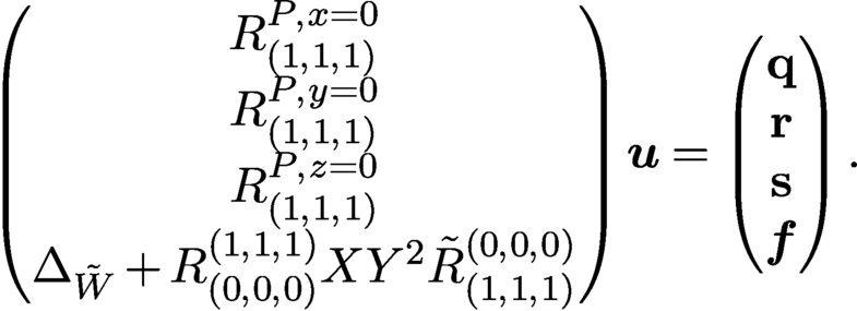 $$ \begin{align*} \begin{pmatrix}R_{(1,1,1)}^{P,x=0}\\ R_{(1,1,1)}^{P,y=0}\\ R_{(1,1,1)}^{P,z=0}\\ \Delta_{\tilde W} + R_{(0,0,0)}^{(1,1,1)} X Y^2 \tilde R_{(1,1,1)}^{(0,0,0)}\end{pmatrix} \boldsymbol{u} = \begin{pmatrix}\mathbf q\\ \mathbf r\\ \mathbf s\\ \boldsymbol{f}\end{pmatrix}. \end{align*} $$
Neumann and Robin conditions can be incorporated by writing the PDE as a system of first-order PDEs, reducing these conditions to Dirichlet.
6.6 p-finite element methods
The Beuchler and Schöberl (Reference Beuchler and Schöberl2006) p-FEM on a triangle was originally constructed directly using Jacobi polynomial relationships to evaluate the corresponding inner products. Instead, as in Section 5.3, we use the quasimatrix notation to manipulate recurrence relationships and thereby construct the p-FEM discretization. While we present the construction on a triangle, it is straightforward to derive a similar method on rectangles and disks.
Following the one-dimensional construction in Section 5.3, we write u and v in terms of weighted OPs on the right-angled triangle as
 $$ \begin{align*} u =xyz \boldsymbol{P}^{(1,1,1)} \boldsymbol{u} \quad\text{and}\quad v = x y z \boldsymbol{P}^{(1,1,1)} \boldsymbol{v}, \end{align*} $$
where
 $z = 1-x-y$
. Then we have
 $$ \begin{align*} \langle \nabla v, \nabla u\rangle = \boldsymbol{v}^{\top} (\nabla w \boldsymbol{P}^{(1,1,1)})^{\top} \nabla x y z \boldsymbol{P}^{(1,1,1)} \boldsymbol{u}. \end{align*} $$
But we also have
 $$ \begin{align*} \nabla xyz \boldsymbol{P}^{(1,1,1)} = \begin{pmatrix}\partial_x xyz \boldsymbol{P}^{(1,1,1)}\\ \partial_y xyz \boldsymbol{P}^{(1,1,1)}\end{pmatrix} = \begin{pmatrix}\boldsymbol{P}^{(0,0,0)} W_{x,(1,1,1)}^{(0,0,0)}\\ \boldsymbol{P}^{(0,0,0)} W_{y,(1,1,1)}^{(0,0,0)}\end{pmatrix} . \end{align*} $$
Lowering down to
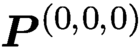 $\boldsymbol {P}^{(0,0,0)}$
, we arrive at a sparse discretization of the weak Laplacian:
 $$ \begin{align*} & (\nabla xyz \boldsymbol{P}^{(1,1,1)})^{\top} \nabla xyz \boldsymbol{P}^{(1,1,1)} \\ &\quad = (W_{x,(1,1,1)}^{(0,0,0)})^{\top} M W_{x,(1,1,1)}^{(0,0,0)} + (W_{y,(1,1,1)}^{(0,0,0)})^{\top} M W_{y,(1,1,1)}^{(0,0,0)} {,} \end{align*} $$
where
 $$ \begin{align*} {M = M_{(0,0,0)} = (\boldsymbol{P}^{(0,0,0)})^{\top} \boldsymbol{P}^{(0,0,0)}} \end{align*} $$
is the diagonal mass matrix corresponding to Legendre polynomials on the triangle; see Proposition B.1. This discretization is symmetric and banded-block-banded with the same sparsity structure as the ultraspherical spectral method, as depicted in Figure 6.3.
6.6.1 Example: ‘good’ and ‘bad’ Helmholtz equations
A nice feature of p-FEM is that it preserves symmetry and positive definiteness, with the latter allowing for efficient Cholesky factorizations. To demonstrate this, we consider the inhomogeneous, variable coefficient Helmholtz equation
 $$ \begin{align} {u^{\prime\prime} + k (1+x y^2) u = 1} \end{align} $$
with zero Dirichlet conditions. When
 $k < 0$
, we call this the ‘good’ Helmholtz equation as it is symmetric positive definite (SPD) and forms boundary layers. In contrast, for
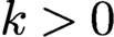 $k> 0$
, the solution is highly oscillatory, and the operator is not positive definite but is still self-adjoint. For
 $k = 0$
, this reduces to the Poisson equation.
In Figure 6.4 we depict solutions for
 $k= -50^2,0,50^2$
showing the transition from boundary layers to oscillations. In Figure 6.5 we show the coefficients for
 $k = -200^2, 0, 200^2$
, which show that the corner singularities drive algebraic decay. At the same time, the boundary layers and oscillations generate slow decay of a different nature. Thus, for moderate k, it is the corner singularities that dictate convergence. In Figure 6.6 we show the timings in building, factorizing and inverting the system. For
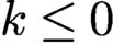 $k \leq 0$
the operator is symmetric negative definite, and a Cholesky factorization is used, while for
 $k> 0$
the operator is only symmetric and an
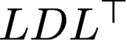 $LDL^{\top }$
factorization is used. We use SuiteSparse to compute the factorizations, which demonstrates an apparent better complexity for Cholesky factorizations, though this may be lost for higher N.
The ‘good’ with
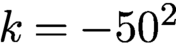 $k=-50^2$
(a), Poisson with
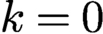 $k = 0$
(b) and ‘bad’ with
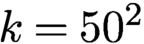 $k = 50^2$
(c) solutions to the inhomogeneous Helmholtz equation (6.4).
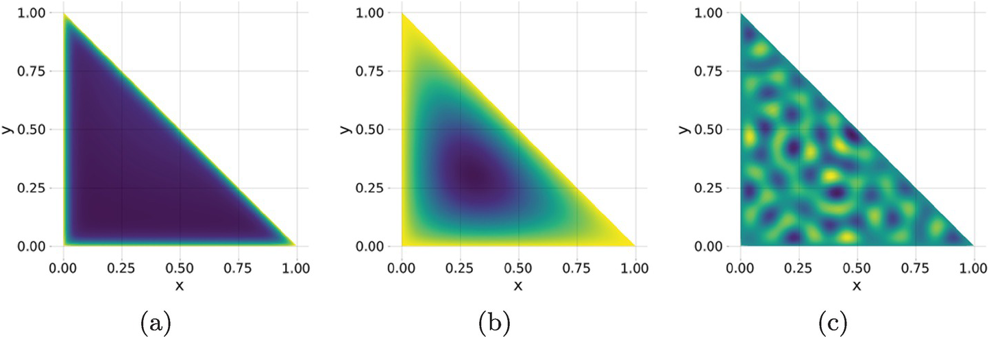
The coefficients for the ‘good’ with
 $k = -200^2$
(a), Poisson with
 $k = 0$
(b) and ‘good’ with
 $k = 200^2$
(c) solutions to the inhomogeneous Helmholtz equation (6.4).
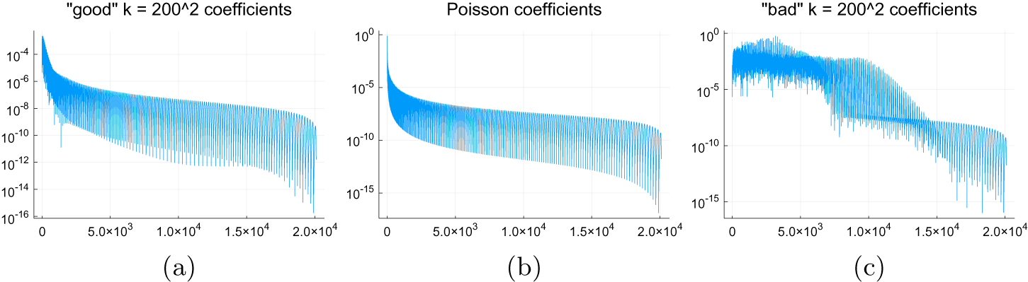
The timings for the ‘good’ with
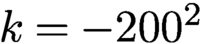 $k = -200^2$
(a), Poisson with
 $k = 0$
(b) and ‘bad’ with
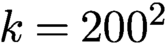 $k = 200^2$
(c) solutions to build, factorize and invert the inhomogeneous Helmholtz equation (6.4). For
 $k \leq 0$
the operator is symmetric negative definite and a Cholesky factorization is used, while for
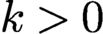 $k> 0$
the operator is only symmetric and an
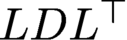 $LDL^{\top }$
factorization is used.
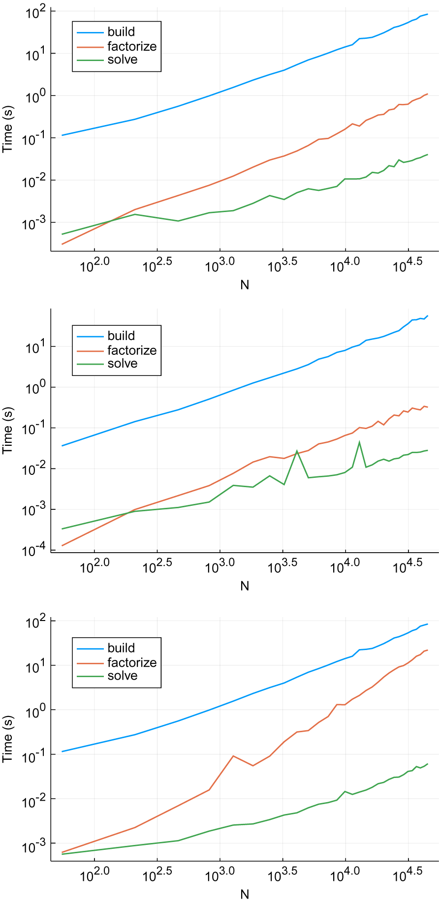
6.7 Domain decomposition
The tools developed lead naturally to a method for solving PDEs on triangle meshes. For the ultraspherical spectral method, this is achieved by imposing continuity in value and derivative over the boundary and reformulating the problem to a system of first-order PDEs. We refer the reader to Olver et al. (Reference Olver, Townsend and Vasil2019) for further details. Figure 6.7 demonstrates these techniques on a Helmholtz equation on a polygon, by subdividing into triangles and imposing continuity up to normal derivatives between each element.
A solution to the Helmholtz equation on a polygon. Figure reproduced from Olver et al. (Reference Olver, Townsend and Vasil2019) with permission. Copyright © 2019 Society for Industrial and Applied Mathematics. All rights reserved.
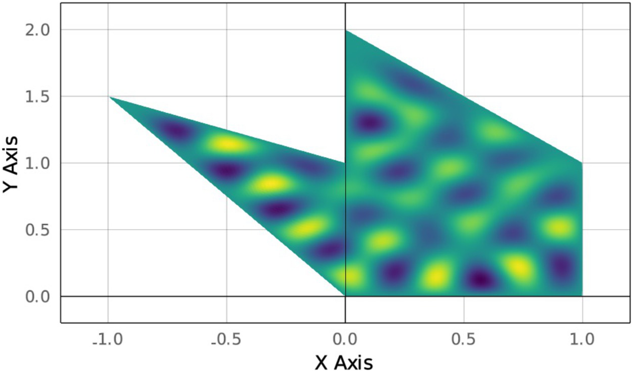
For the p-FEM, this is achieved by using the basis
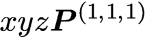 $x y z \boldsymbol {P}^{(1,1,1)}$
in each element as the bubble functions. Face bubble functions are then added between adjoining elements: for example, if we have two triangles, one on top of the other with adjoining edge from
 $(0,0)$
to
 $(1,0)$
, on the interface we have
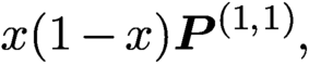 $$ \begin{align*} x (1-x) \boldsymbol{P}^{(1,1)}, \end{align*} $$
which can be extended to the triangles as
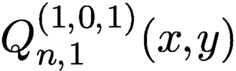 $Q_{n,1}^{(1,0,1)}(x,y)$
, which vanishes on the other two edges. This extension can then be differentiated and converted as appropriate. We refer the reader to Beuchler and Schöberl (Reference Beuchler and Schöberl2006) for more details.
7 Singular integral equations
Singular integral equations arise in potential theory, boundary integral reformulations of partial differential equations, and elsewhere. Conventional numerical methods typically involve discretization of the geometry using either quadrature rules (à la Nyström method) or collocation points, though these methods must deal with singularities in the integrals. A recent success story along these lines is the quadrature-by-expansion (QBX) method of Klöckner, Barnett, Greengard and O’Neil (Reference Klöckner, Barnett, Greengard and O’Neil2013).
As an alternative in two dimensions (i.e. one-dimensional singular integral equations corresponding to two-dimensional PDEs), we advocate using weighted OPs to calculate the singular integrals exactly via recurrence relationships. Cauchy transforms of weighted OPs satisfy the same recurrence relationship as the OPs themselves, which has been used successfully in numerical computing going back to Elliott (Reference Elliott1982) and Gautschi and Wimp (Reference Gautschi and Wimp1987). Less well known is that this is applicable for logarithmic singularities as well. Slevinsky and Olver (Reference Slevinsky and Olver2017) used these relationships, which show that singular integral operators are banded on a single interval, to construct an ultraspherical spectral method for solving singular integral equations. Multiple scattered plates can also be tackled using low-rank techniques, and more complicated smooth arcs using suitable change-of-variables formulas.
7.1 Cauchy and Hilbert transforms
The Cauchy transform over a contour
 $\Gamma $
is denoted by
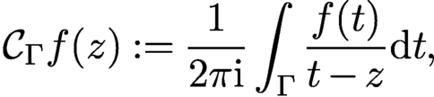 $$ \begin{align} {\mathcal C}_\Gamma f(z) := \displaystyle \frac{1 }{ 2 \pi {\mathrm{i}}} \int_\Gamma \displaystyle \frac{f(t) }{ t - z}{\mathrm{d}} t, \end{align} $$
which is analytic for
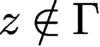 $z \notin \Gamma $
. Provided it has well-defined left and right limits (which is the case for reasonable functions f, e.g. smooth functions times Jacobi weights on
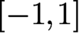 $[-1,1]$
), we use the notation
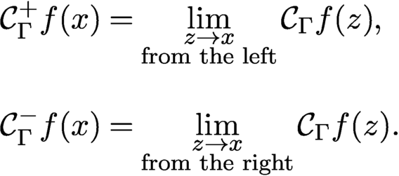 $$ \begin{align*} {\mathcal C}_\Gamma^+ f(x) & = \lim_{{\substack{z \rightarrow x \\ \text{from the left}}}} {\mathcal C}_\Gamma f(z), \\[10pt] {\mathcal C}_\Gamma^- f(x) & = \lim_{{\substack{z \rightarrow x \\ \text{from the right}}}} {\mathcal C}_\Gamma f(z). \end{align*} $$
We omit the subscript
 $\Gamma $
when it is implied by the context.
Since Cauchy transforms are themselves just integrals, they can be discretized via a quadrature rule. That is,
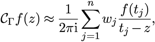 $$ \begin{align} {\mathcal C}_\Gamma f(z) \approx \displaystyle \frac{1 }{ 2 \pi {\mathrm{i}}} \sum_{j=1}^n w_j \displaystyle \frac{f(t_j) }{ t_j - z}, \end{align} $$
where
 $\{t_j\}$
and
 $\{w_j\}$
are quadrature nodes and weights for the contour
 $\Gamma $
. However, this is not a good idea for Cauchy transforms as they are singular integrals. In particular, the quantity on the left-hand side of (7.2) has a branch cut while the right-hand side of (7.2) has poles. We may need to evaluate the singular integral on or near
 $\Gamma $
, where the quadrature rule is not accurate. We visualize this using a phase portraitFootnote
8
in the style of Wegert (Reference Wegert2012) in Figure 7.1. The true Cauchy transform has a branch cut on the interval, whereas Gauss quadrature results in poles along the branch cut.
The Cauchy transform of
 ${\mathrm {e}}^x$
over
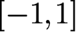 $[-1,1]$
computed using Legendre polynomials (a) compared to Gauss–Legendre quadrature (b). The Legendre polynomial-based approximation is uniformly accurate to roughly machine precision up to and on the interval. In contrast, the quadrature-based approach is not accurate on the contour itself, and has introduced artificial poles.
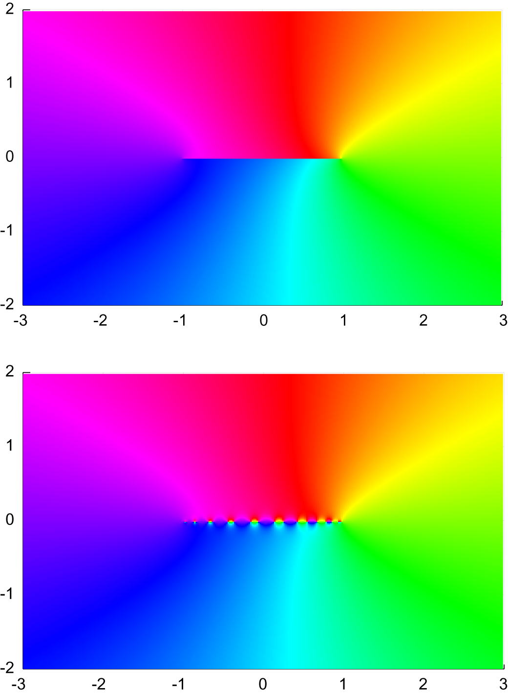
As an alternative, we propose first expanding the integrand f in (7.1) in a weighted OP basis. Once an expansion is known, we have a natural approximation to the Cauchy transform:
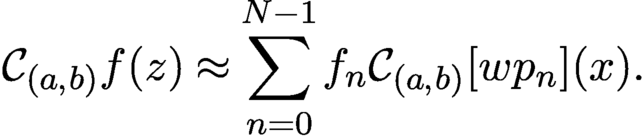 $$ \begin{align*} {\mathcal C}_{(a,b)} f(z) \approx \sum_{n=0}^{N-1} f_n {\mathcal C}_{(a,b)}[w p_n](x). \end{align*} $$
The approximation on the right has a jump on the interval of orthogonality
 $[a,b]$
matching the true Cauchy transform. In fact, in a certain sense, we achieve uniform convergence (though we omit details), and therefore we can approximate the Cauchy transform up to and on the jump.
The calculation of a general Cauchy transform is reduced to one involving the generation of weighted OPs. Fortunately, Cauchy transforms satisfy a recurrence relationship that makes them straightforward to evaluate. Let
 $$ \begin{align*} C_n(z) := {\mathcal C}_{(a,b)}[p_n w](z). \end{align*} $$
Then we have
 $$ \begin{align*} z C_0(z) &= a_0 C_0(z) + b_0 C_1(z) - \displaystyle \frac{1 }{ 2 \pi {\mathrm{i}}} \int_a^b w(x) {{\mathrm{d}}x}, \\ z C_n(z) &= c_n C_{n-1}(z) + a_n C_n(z) + b_n C_{n+1}(z), \quad n\geq 1. \end{align*} $$
This well-known formula (see e.g. Gautschi Reference Gautschi1981b ) is derived by the following simple calculation:
 $$ \begin{align*} z C_n(z) &= \displaystyle \frac{1 }{ 2 \pi {\mathrm{i}}} \int_a^b \displaystyle \frac{(z -x) p_n(x) w(x) }{ x -z} {{\mathrm{d}}x} + \int_a^b \displaystyle \frac{x p_n(x) w(x) }{ x -z} {{\mathrm{d}}x} \\ &= -\displaystyle \frac{1 }{ 2 \pi {\mathrm{i}}} \int_a^b p_n(x) w(x) {{\mathrm{d}}x} + c_n C_{n-1}(z) + a_n C_n(z) + b_n C_{n+1}(z). \end{align*} $$
Note that the integral term is zero when
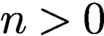 $n> 0$
.
The key feature of this recurrence is that if we know
 $C_0(z) ={\mathcal C}w(z)$
and
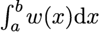 $\int _a^b w(x) {{\mathrm {d}}x}$
, then we can determine
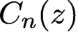 $C_n(z)$
by solving the following lower-triangular system using forward substitution:
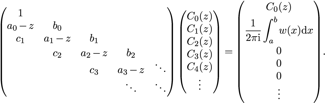 $$ \begin{align*} \begin{pmatrix} 1 \\ a_0-z & b_0 \\ c_1 & a_1-z & b_1 \\[2pt] &c_2 & a_2-z & b_2 \\[-3pt] && c_3 & a_3-z &\ddots\\ &&&\ddots & \ddots \end{pmatrix} \begin{pmatrix}C_0(z) \\ {C}_1(z) \\ {C}_2(z) \\ {C}_3(z) \\ C_4(z)\\ \vdots \end{pmatrix} = \begin{pmatrix}C_0(z) \\[3pt] \displaystyle \frac{1 }{ 2 \pi {\mathrm{i}}} \int_a^b w(x) {{\mathrm{d}}x} \\[8pt] 0 \\0 \\ 0\\ \vdots \end{pmatrix}\!. \end{align*} $$
This recurrence-based approach also extends to the Hilbert transform Footnote 9 given by
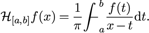 $$ \begin{align} {\mathcal H}_{[a,b]} f(x) = \displaystyle \frac{1 }{ \pi} {\int\!\!\!\!\!\!-}_a^b \displaystyle \frac{f(t) }{ x-t} {{\mathrm{d}}t}. \end{align} $$
By the Plemelj theorem, the Hilbert and Cauchy transforms are related by (Muskhelishvili Reference Muskhelishvili1953, Trogdon and Olver Reference Trogdon and Olver2016)
 $$ \begin{align*} {\mathcal C}^+ - {\mathcal C}^- = I,\quad {\mathcal C}^+ + {\mathcal C}^- = {\mathrm{i}} {\mathcal H}. \end{align*} $$
Therefore, the recurrence relationships for Cauchy transforms of OPs immediately imply one for Hilbert transforms of OPs. Let
 $$ \begin{align*} H_n(z) := {\mathcal H}[p_n w](z). \end{align*} $$
Then we have
 $$ \begin{align*} x H_0(x) &= a_0 H_0(x) + b_0 H_1(x) + \displaystyle \frac{1 }{ \pi} \int_a^b w(x) {{\mathrm{d}}x},\\[-3pt] x H_n(x) &= c_n H_{n-1}(x) + a_n H_n(x) + b_n H_{n+1}(x), \quad n\geq 1. \end{align*} $$
7.1.1 Example: Hilbert transforms of Chebyshev polynomials
Consider the Hilbert transform of the Chebyshev polynomial
 $T_n$
, that is,
 $$ \begin{align*} {H_n(x) = \displaystyle \frac{1 }{ \pi} {\int\!\!\!\!\!\!-}_{-1}^1 \displaystyle \frac{T_n(t) }{ (x-t)\sqrt{1-t^2}} {{\mathrm{d}}t}.} \end{align*} $$
The recurrence relationship satisfied by
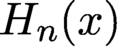 $H_n(x)$
is
 $$ \begin{align*} x H_0(x) = H_1(x) +1, \quad x H_n(x) = \displaystyle \frac{H_{n-1}(x) }{ 2} + \displaystyle \frac{H_n(x) }{ 2}, \quad n\geq 1. \end{align*} $$
In this case we have
 $H_0(x) = {\mathcal H}[(1-t^2)^{-1/2}](x) = 0.$
Therefore we have
 $$ \begin{align*} H_1(x)= -1, \quad H_2(x) = -2x, \quad H_{n+1}(x) = 2xH_n(x) - H_{n-1}(x). \end{align*} $$
This is precisely the three-term recurrence relationship satisfied by the Chebyshev polynomials (of the second kind). Due to the values for
 $H_0$
and
 $H_1$
, we find that
 $H_n(x) = -U_{n-1}(x)$
for
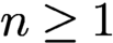 $n\geq 1$
. In quasimatrix notation, we have
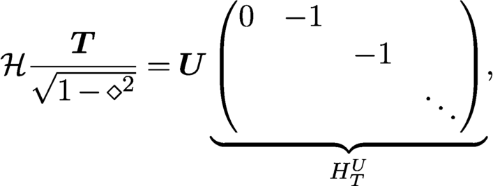 $$ \begin{align*} {\mathcal H} \displaystyle \frac{\boldsymbol{T} }{ \sqrt{1-\diamond^2}} = \boldsymbol{U} \underbrace{\begin{pmatrix}0 & -1\\ && -1 \\ &&&\ddots \end{pmatrix}}_{H_T^U}\!{,} \end{align*} $$
where
 $\diamond $
denotes the ‘dummy’ variable.
A related formula holds for the Hilbert transform of Chebyshev polynomials of the second kind, where the fact that
 ${\mathcal H}[\sqrt {1-\diamond ^2}](x) = 1$
leads to
 ${\mathcal H}[\sqrt {1-\diamond ^2} U_n] = T_{n+1}(x)$
for
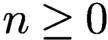 $n\geq 0$
. In quasimatrix notation, we have
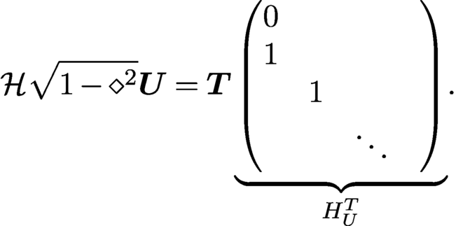 $$ \begin{align*} {\mathcal H} \sqrt{1-\diamond^2} \boldsymbol{U} = \boldsymbol{T} \underbrace{\begin{pmatrix}0 \\ 1\\ & 1 \\ && \ddots & \end{pmatrix}}_{H_U^T}\!. \end{align*} $$
7.2 Inverting shifted Jacobi operators and Cauchy transforms
While forward recurrence is an effective approach for calculating Cauchy transforms, it can run into numerical stability issues if the evaluation point is far from
 $[a,b]$
: Cauchy transforms and OPs satisfy the same recurrence relationship (they are the minimal and maximal solutions, respectively) apart from the initial conditions. Any small perturbation to the initial condition for the minimal solution will pick up the maximal solution, which blows up as
 $n \rightarrow \infty $
. On the other hand,
 $C_n(z) \rightarrow 0$
as
 $n \rightarrow \infty $
for z off the support of w.
There are effective methods for calculating minimal solutions to recurrence relationships. We have
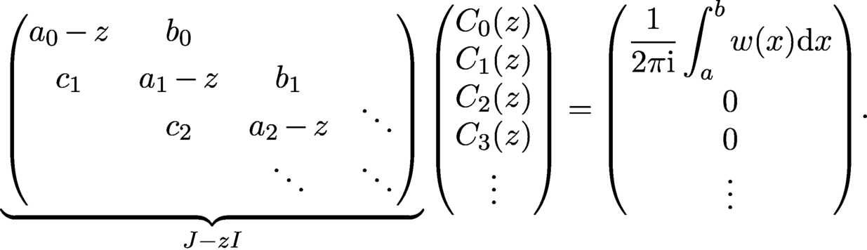 $$ \begin{align} \underbrace{\begin{pmatrix} a_0-z & b_0 \\[3pt] c_1 & a_1-z & b_1 \\[-4pt] & c_2 & a_2-z &\ddots\\ &&\ddots & \ddots \end{pmatrix}}_{J - z I} \begin{pmatrix}C_0(z) \\ C_1(z) \\ {C}_2(z) \\ {C}_3(z) \\ \vdots \end{pmatrix} = {\begin{pmatrix} \displaystyle \frac{1}{2\pi {\mathrm{i}}} \int_a^b w(x) {{\mathrm{d}}x} \\[8pt] 0 \\0 \\ \vdots \end{pmatrix}\!.} \end{align} $$
The operator
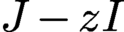 $J -z I$
is invertible in
 $\ell ^2$
(assuming J is bounded) when z is not on the spectrum of J, which is precisely the support of the weight, the interval
 $[a,b]$
. This means that the Cauchy transform is the unique solution to (7.4). As discussed in Section 5, there are multiple ways of solving an infinite-dimensional linear system such as (7.4), with Olver’s algorithm being particularly attractive as it is fast, stable and adaptive.
There is a remaining question of when to use forward recurrence or directly inverting
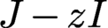 $J - z I$
. As z approaches
 $[a,b]$
, the decay rate of
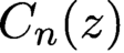 $C_n(z)$
degenerates, which requires computing an increasing number of terms to achieve convergence. In lockstep, the forward recurrence becomes increasingly stable to use. In practice we find that the following heuristic works well: if one requires the first
 $C_0(z),\ldots ,C_N(z)$
for a specified value N, use forward recurrence if N is in a Bernstein ellipse with radii proportional to
 $1/N$
; otherwise, invert
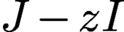 $J-zI$
.
7.3 Log transforms
From the Green’s function of the Laplacian, it is natural to consider integrals with a logarithmic kernel. If
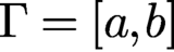 $\Gamma = [a,b]$
, then the log transform is defined by
 $$ \begin{align*}{\mathcal L} f(z) = \displaystyle \frac{1 }{ \pi }\int_a^b f(t) \log | z - t| {{\mathrm{d}}t}{,}\end{align*} $$
where now we assume f is real-valued. It turns out that logarithmic singular integrals satisfy a simple recurrence relationship for weighted classical orthogonal polynomials, which we show by relating them to Cauchy transforms.
For
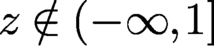 $z \notin (-\infty ,1]$
, we use the following formula:
 $$ \begin{align*} v(z) = {\text{Re}\,} \displaystyle \frac{1 }{ \pi} \int_a^b f(t) \log ( z - t) {{\mathrm{d}}t}. \end{align*} $$
(Note that the integrand avoids the branch cut of
 $\log z$
.) To extend this to
 $z\in (-\infty ,-1]$
(or more generally,
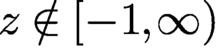 $z \notin [-1,\infty )$
), we can use the alternative expression given by
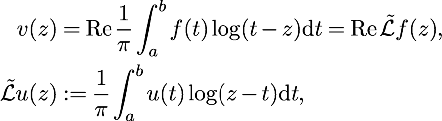 $$ \begin{align*} v(z) & = {\text{Re}\,} \displaystyle \frac{1 }{ \pi} \int_a^b f(t) \log (t-z) {{\mathrm{d}}t} = {\text{Re}\,} \tilde {\mathcal L} f(z),\\ \tilde {\mathcal L} u(z) & := \displaystyle \frac{1 }{ \pi} \int_a^b u(t) \log (z-t) {{\mathrm{d}}t}, \end{align*} $$
which follows from the fact that
 $\log |z-t| = \log |t-z|$
.
To evaluate
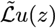 $\tilde {\mathcal L} u(z)$
in the complex plane we use the following expressionFootnote
10
in terms of Cauchy transforms:
 $$ \begin{align} \tilde {\mathcal L} u(z) = \displaystyle \frac{\log(z-a) }{ \pi} \int_a^b u(x) {{\mathrm{d}}x} +2 {\mathrm{i}} {\mathcal C} U(z), \quad U(x) = \int_x^b u(t) {{\mathrm{d}}t}. \end{align} $$
As the indefinite integral of classical orthogonal polynomials is also orthogonal, we arrive at a closed-form expression in terms of Cauchy transforms of orthogonal polynomials.
7.3.1 Example: log kernel of Legendre, Chebyshev and Jacobi polynomials
Consider
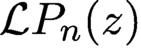 ${\mathcal L} P_n(z)$
. For
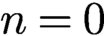 $n = 0$
we have
 $$ \begin{align*} \tilde {\mathcal L} 1(z) = \displaystyle \frac{2 \log(z+1) }{ \pi} + 2 {\mathrm{i}} {\mathcal C}[x-1](z). \end{align*} $$
For
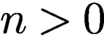 $n> 0$
the definite integral is zero due to orthogonality and we have an explicit expression for the indefinite integral from Proposition A.6, which gives us
 $$ \begin{align*} \tilde {\mathcal L} P_n(z) = -\displaystyle \frac{{\mathrm{i}} }{ n} {\mathcal C}[(1-\diamond^2) P_{n-1}^{(1,1)}](z), \quad n\geq 1. \end{align*} $$
Taking the real part of
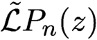 $\tilde {\mathcal L} P_n(z)$
gives
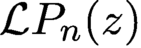 ${\mathcal L} P_n(z)$
for all n.
For Chebyshev polynomials, we have for
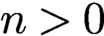 $n> 0$
, using Proposition A.16,
 $$ \begin{align*} \int_x^1 \displaystyle \frac{{T_n (t)}}{ \sqrt{1-t^2}} {{\mathrm{d}}t} = -\displaystyle \frac{U_{n-1}(x) }{ n} \sqrt{1-x^2} \end{align*} $$
so that
 $$ \begin{align*} \tilde {\mathcal L} \biggl[\dfrac{T_n }{ \sqrt{1-\diamond^2}}\biggr](z) = -\displaystyle \frac{2 {\mathrm{i}} }{ n+1} {\mathcal C}\bigl[\sqrt{1-\diamond^2} U_{n-1}\bigr](z). \end{align*} $$
We are left with the
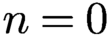 $n=0$
case, but this can be calculated explicitly as
 $$ \begin{align*} {\mathcal L} [(1-\diamond^2)^{-1/2}](z) = - \log {|J_+^{-1}(z)|} - \log 2 \end{align*} $$
using the fact that
 $$ \begin{align*} \int^z \displaystyle \frac{1 }{ \sqrt{z-1} \sqrt{z+1}} {{\mathrm{d}}z} = - \log J_+^{-1}(z), \end{align*} $$
where
 $J_+^{-1}(z) = z - \sqrt {z-1} \sqrt {z+1}$
is a pre-image of the Joukowsky transform
 $z\mapsto (z+z^{-1})/2$
.
A nice consequence of this is the following beautiful formula for evaluating on the interval
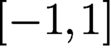 $[-1,1]$
:
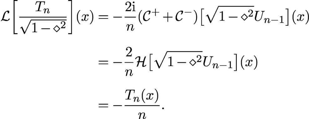 $$ \begin{align*} {\mathcal L}\biggl[\displaystyle \frac{T_n }{ \sqrt{1-\diamond^2}}\biggr] (x) & = -\displaystyle \frac{2 {\mathrm{i}} }{ n} ({\mathcal C}^+ + {\mathcal C}^-)\bigl[\sqrt{1-\diamond^2} U_{n-1}\bigr] (x) \\[6pt] &= -\displaystyle \frac{2 }{ n} {\mathcal H} \bigl[\sqrt{1-\diamond^2} U_{n-1}\bigr](x) \\[6pt] & = -\displaystyle \frac{{T_n (x)}}{ n}. \end{align*} $$
For the
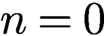 $n=0$
case we have
 $$ \begin{align*} {\mathcal L} [(1-\diamond^2)^{-1/2}] (x) = - \log 2. \end{align*} $$
Putting everything together, we arrive atFootnote 11
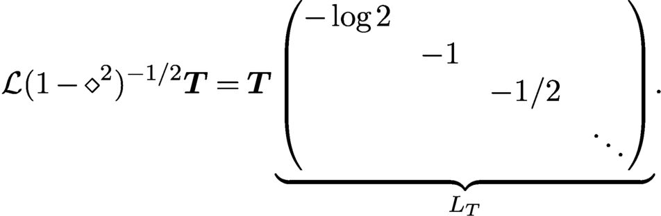 $$ \begin{align*} {\mathcal L} (1-\diamond^2)^{-1/2} \boldsymbol{T} = \boldsymbol{T} \underbrace{\begin{pmatrix}-\log 2 \\ & -1 \\ && -1/2 \\ &&& \ddots \end{pmatrix}}_{{L_T}}\!. \end{align*} $$
Finally, we find that the relationship
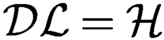 ${\mathcal D} {\mathcal L} = {\mathcal H}$
translates to
 $$ \begin{align*} {\mathcal H} {\mathcal L} (1-\diamond^2)^{-1/2} \boldsymbol{T} = {\mathcal D} {\mathcal L} (1-\diamond^2)^{-1/2} \boldsymbol{T} = {\mathcal D} \boldsymbol{T} L_T = \boldsymbol{U} D_T^U L_T = \boldsymbol{U} H_T^U. \end{align*} $$
Extension to other Jacobi polynomials is straightforward, though the
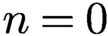 $n = 0$
case often involves hypergeometric functions:
 $$ \begin{align} {\mathcal L}_{\mathbb{I}}w^{(\alpha,\beta)}(z) & = \displaystyle \frac{2^{\alpha+\beta+1}{\mathrm B}(\alpha+1,\beta+1) }{ \pi} \bigg\{\log(z-1)\\ & \quad\, +\dfrac{\alpha+1}{\alpha+\beta+2}\bigg(\dfrac{2}{z-1}\bigg) {}_{3}F_{2}\bigg(\begin{array}{c} 1,1,\alpha+2\\2,\alpha+\beta+3\end{array}; \dfrac{2}{1-z}\bigg)\bigg\},\nonumber\\[-10pt]\nonumber \end{align} $$
which comes from integrating the Cauchy transforms of the Jacobi weight, and where
 ${\mathrm B}$
is the Beta function (Olver et al. Reference Olver, Lozier, Boisvert and Clark2010, §5.12). This integration essentially follows from
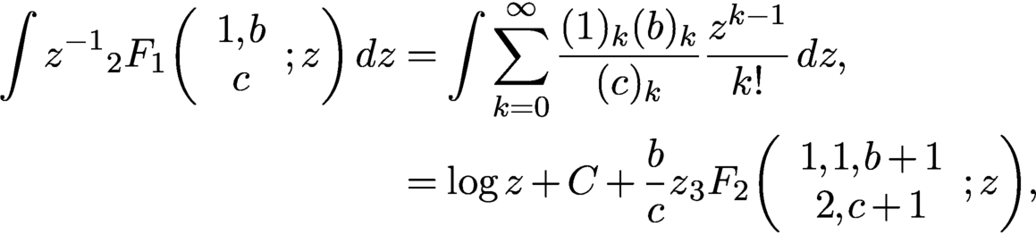 $$ \begin{align*} \int z^{-1}{}_{2}F_{1}\bigg(\begin{array}{c}1,b\\c\end{array};z\bigg){\mathrm\,d} z & = \int\sum_{k=0}^\infty \dfrac{(1)_k(b)_k}{(c)_k}\dfrac{z^{k-1}}{k!}{\mathrm\,d} z,\\ & = \log z + C + \dfrac{b}{c}z {}_{3}F_{2}\bigg(\begin{array}{c}1,1,b+1\\2,c+1\end{array};z\bigg), \end{align*} $$
where the constant is determined by the asymptotic behaviour at infinity.
Since generalized hypergeometric functions are challenging to compute near the branch cut, we identify this particular one with a partial derivative with respect to a parameter of a Gaussian hypergeometric function. Together with forward-mode automatic differentiation, this avoids numerical difficulties near the branch cut:
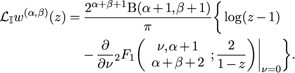 $$ \begin{align*} {\mathcal L}_{\mathbb{I}}w^{(\alpha,\beta)}(z) & = \displaystyle \frac{2^{\alpha+\beta+1}{\mathrm B}(\alpha+1,\beta+1) }{ \pi} \bigg\{\log(z-1)\\ & \quad\, -\dfrac{\partial}{\partial \nu} {}_{2}F_{1}\bigg(\begin{array}{c} \nu,\alpha+1\\\alpha+\beta+2\end{array}; \dfrac{2}{1-z}\bigg)\bigg|_{\nu=0}\bigg\}.\nonumber \end{align*} $$
This formula is the result of taking the limit as
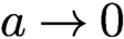 $a\to 0$
below and using Olver et al. (Reference Olver, Lozier, Boisvert and Clark2010, §15.5.3) and l’Hôpital’s rule:
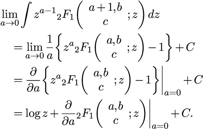 $$ \begin{align*} &\lim_{a\to0}\int z^{a-1}{}_{2}F_{1}\bigg(\begin{array}{c}a+1,b\\c\end{array};z\bigg){\mathrm\,d} z \\ & \quad = \lim_{a\to0}\dfrac{1}{a}\bigg\{z^a {}_{2}F_{1}\bigg(\begin{array}{c}a,b\\c\end{array};z\bigg)-1\bigg\} + C \\ &\quad = \dfrac{\partial}{\partial a}\bigg\{z^a{}_{2}F_{1}\bigg(\begin{array}{c}a,b\\c\end{array};z\bigg)-1\bigg\}\bigg|_{a=0} + C \\ &\quad = \log z + \dfrac{\partial}{\partial a}{}_{2}F_{1}\bigg(\begin{array}{c}a,b\\c\end{array};z\bigg)\bigg|_{a=0} + C. \end{align*} $$
7.4 Ultraspherical spectral methods for singular integral operators
There is a natural way of discretizing singular integral operators using sparse matrices (Slevinsky and Olver Reference Slevinsky and Olver2017). On a single interval this involves using the following quasimatrix relationships:
 $$ \begin{align*} {\mathcal H} (1-\diamond^2)^{-1/2} \boldsymbol{T} = \boldsymbol{U} H_T^U \quad\text{and}\quad {\mathcal L} (1-\diamond^2)^{-1/2} \boldsymbol{T} = \boldsymbol{T} L_T. \end{align*} $$
Note that this also gives a way of calculating hyper-singular integrals. For example,
 $$ \begin{align*} {\mathcal D} {\mathcal H} (1-\diamond^2)^{-1/2} \boldsymbol{T} = \boldsymbol{C}^{(2)} D_U^{(2)} H_T^U. \end{align*} $$
7.4.1 Example: the potential field of a metal sheet
As a simple example, consider the solution of the following Laplace equation, where
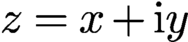 $z = x + {\mathrm {i}} y$
:
-
(1)
$v_{xx} + v_{yy} = 0 $
for
$z \notin [-1,1] \cup \{{\mathrm {i}} \epsilon \}$
, -
(2)
$ v(x,y) = \log |z - {\mathrm {i}} \epsilon | + O({1}) $
as
$z \rightarrow {\mathrm {i}} \epsilon $
, -
(3)
$ v(x,y) = o(1) $
as
$z \rightarrow \infty $
, and -
(4)
$ v(x,0) = \kappa $
for
$-1 < x < 1$
, where
$\kappa $
is an unknown constant.



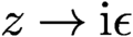

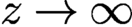
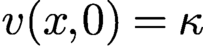


This equation models the potential field of a unit charge located at
 ${\mathrm {i}} \epsilon $
with a metal sheet that has no net charge placed on
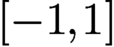 $[-1,1]$
. As an ansatz for v, we write
 $$ \begin{align*} v(z) = {\mathcal L} u(z) + \log|z - {\mathrm{i}} \epsilon|, \end{align*} $$
which reduces the problem to one involving the following singular integral equation:
 $$ \begin{align*} v(x,0) = {\mathcal L} u(x) = \kappa - \log|x - {\mathrm{i}} \epsilon|, \quad -1 < x < 1,\quad \int_a^b u(x) = 0. \end{align*} $$
By writing
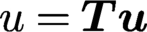 $u = \boldsymbol {T} \boldsymbol {u}$
, this becomes an almost diagonal linear system
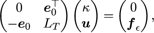 $$ \begin{align} \begin{pmatrix}0 & \boldsymbol{e}_0^{\top}\\ -\boldsymbol{e}_0 & L_T \end{pmatrix} \begin{pmatrix}\kappa \\ \boldsymbol{u}\end{pmatrix} = \begin{pmatrix}0\\ \boldsymbol{f}_\epsilon\end{pmatrix}, \end{align} $$
where
 $-\log |x - {\mathrm {i}} \epsilon | = \boldsymbol {T}(x) \boldsymbol {f}_\epsilon $
. Analyticity ensures that
 $\boldsymbol {f}_\epsilon $
has
 $N = O({1/\epsilon })$
coefficients above a prescribed tolerance, which can be calculated in
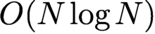 $O({N \log N})$
time, using the Chebyshev transform described in Section 4.1. The coefficients
 $\boldsymbol {u}$
are then determined by solving (7.7), which costs
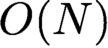 $O({N})$
operations. Finally, we can evaluate
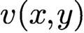 $v(x,y)$
pointwise using the expressions involving the Cauchy transform, which in turn is achieved via the recurrence relationship. We demonstrate this example in Figure 7.2, which depicts the solution with
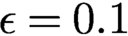 $\epsilon = 0.1$
and shows the number of coefficients needed to resolve the solution for different choices of
 $\epsilon $
, demonstrating the necessity of fast algorithms.
The solution to the Laplace equation with a single point source at
 $0.2 {\mathrm {i}}$
as described in Section 7.4.1 (a), and the coefficients of the solution for
 $\epsilon =0.1,0.01,0.001$
(b). This figure demonstrates the benefits of an
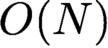 $O({N})$
algorithm when the forcing term is challenging to resolve.
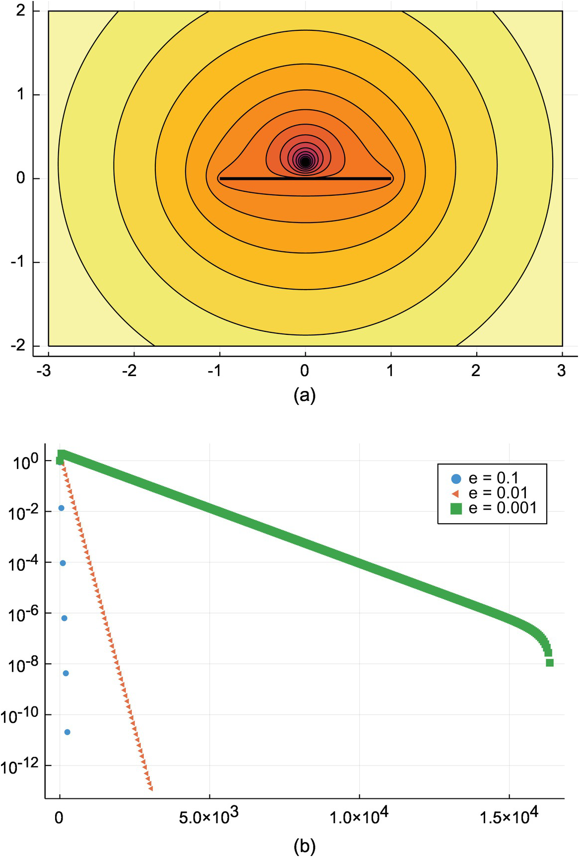
7.4.2 Other kernels
This framework also supports more general kernels such as those arising in elliptic PDEs, with the Helmholtz equation being the canonical case. In this setting, we are guaranteed that the kernel can be written as
 $$ \begin{align*} K_1(x,y) \log|x-y| + \displaystyle \frac{K_2(x,y) }{ x - y} + K_3(x,y), \end{align*} $$
where integration against this kernel is understood in the principal value sense. At this point, we approximate
 $K_m$
by a low-rank function approximation
 $$ \begin{align*} K_m(x,y) \approx \sum_{j=1}^r a_j^m(x) b_j^m(y), \quad m = 1,2,3, \end{align*} $$
where, for simplicity, we assume that the rank, r, does not depend on m. A low-rank approximation of
 $K_m$
can be computed using a singular value decomposition or other low-rank techniques for functions (Townsend and Trefethen Reference Townsend and Trefethen2013). Setting
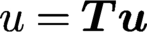 $u = \boldsymbol {T} \boldsymbol {u}$
, we have the following expression for
 $K_1$
:
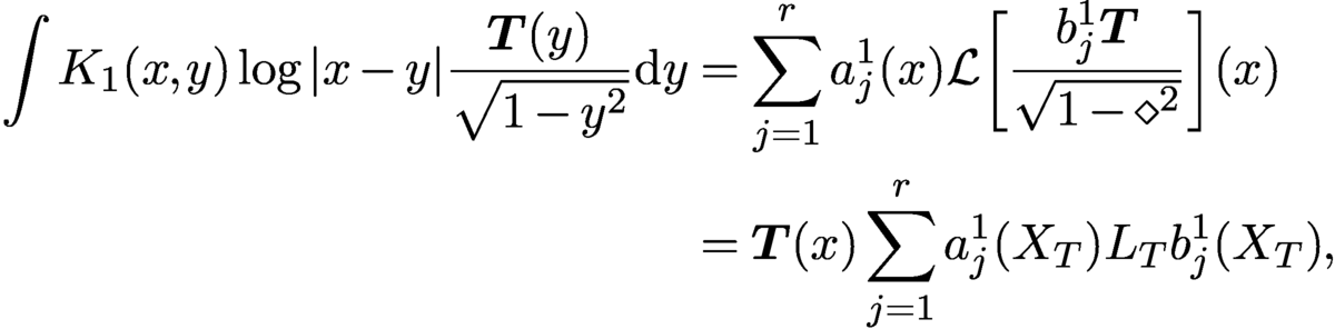 $$ \begin{align*} \int K_1(x,y) \log|x-y| \displaystyle \frac{{\boldsymbol{T} (y)}}{ \sqrt{1-y^2}} {{\mathrm{d}}y} & = \sum_{j=1}^r a_j^1(x) {\mathcal L}\biggl[\displaystyle \frac{b_j^1 \boldsymbol{T} }{ \sqrt{1-\diamond^2}}\biggr](x) \\ & = \boldsymbol{T}(x) \sum_{j=1}^r a_j^1(X_T) L_T b_j^1(X_T), \end{align*} $$
where
 $X_T$
is again the multiplication-by-x operator corresponding to the Chebyshev polynomials
 $\boldsymbol {T}$
. The other kernels are handled similarly, leading to the discretization
 $$ \begin{align*} \boldsymbol{U} \sum_{j=1}^r [R_T^U a_j^1(X_T) L_T b_j^1(X_T) + a_j^2(X_U) H_T^U b_j^1(X_T) + a_j^3(X_U) \boldsymbol{e}_0 \Sigma_T b_j^3(X_T)]. \end{align*} $$
The bandwidth of the discretization depends on the polynomial degree of
 $a_j^m$
and
 $b_j^m$
for
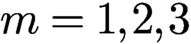 $m = 1,2,3$
. If
 $a_j^m$
and
 $b_j^m$
for
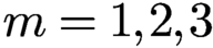 $m = 1,2,3$
are all of degree
 $\leq d$
, then the number of sub/super-diagonals is precisely d.
7.4.3 Example: Helmholtz on an interval
In Figure 7.3(a) we demonstrate an acoustic scattering analogue of the example presented in Section 7.4.1, now with a large number of point scatterers on a Bernstein ellipse surrounding
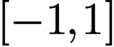 $[-1,1]$
. That is, we wish to solve
 $$ \begin{align*} v_{xx} + v_{yy} + k^2 v = 0 \quad \text{for } z \notin [-1,1] \cup \Gamma_\epsilon, \end{align*} $$
where
 $\Gamma _\epsilon $
consists of the set of point sources on the Bernstein ellipse. An increasing number of coefficients are needed to resolve the solution as the point sources approach the interval, but the resulting banded system can be solved in
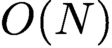 $O(N)$
complexity. This example originally appeared in Slevinsky and Olver (Reference Slevinsky and Olver2017), which also includes timings showing the
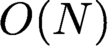 $O(N)$
complexity, where N is the total degrees of freedom needed to resolve the solution.
Acoustic scattering off an interval with many nearby point scatterers (a) and off a metal sheet model of Great Britain (b). Figure reproduced from Slevinsky and Olver (Reference Slevinsky and Olver2017) with permission. Copyright © 2017 Elsevier.
7.5 Multiple segments
So far we have described a systematic approach to solving singular integral equations on
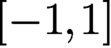 $[-1,1]$
with a similar construction being viable on the unit circle with Laurent series. Similarly, any affine transformation of a line-segment embedded in
 ${\mathbb R}^2$
(or equivalently in
 ${\mathbb C}$
) is straightforward. To solve SIEs posed on multiple intervals/circles, we discretize them in a block-wise manner.
As a simple example, suppose we want to solve Laplace’s equation on the complement of two intervals
 $\Gamma _{-1} := [-2,-1]$
and
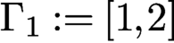 $\Gamma _1 := [1,2]$
and determine an expansion of the solution in the form
 $$ \begin{align*} u(x) = \begin{cases} \sum_{k=0}^\infty u_k (1-(2x+3)^2)^{-1/2} T_k(2x+3) & -1 < x < -2,\\[5pt] \sum_{k=0}^\infty v_k (1-(2x-3)^2)^{-1/2} T_k(2x-3) & 1 < x < 2. \end{cases} \end{align*} $$
Define
 $\boldsymbol {T}_{-1}(x) := \boldsymbol {T}(2x+3)$
and
 $\boldsymbol {T}_1(x) := \boldsymbol {T}(2x-3)$
to be the mapped Chebyshev polynomials with corresponding weights
 $w_{-1}(x) = (1-(2x+3)^2)^{-1/2}$
and
 $w_2(x) = (1-(2x-3)^2)^{-1/2}$
. Using a block-wise version of the quasimatrix notation, we want to solve
 $$ \begin{align*} \begin{pmatrix}{\mathcal L}_{\Gamma_{-1}} & {\mathcal L}_{\Gamma_{1}} |_{\Gamma_{-1}} \\ {\mathcal L}_{\Gamma_{-1}} |_{\Gamma_{1}} & {\mathcal L}_{\Gamma_{1}} \end{pmatrix} \begin{pmatrix} w_{-1} \boldsymbol{T}_{-1} & \\ & w_1 \boldsymbol{T}_1\end{pmatrix} \begin{pmatrix}\boldsymbol{u}_{-1}\\ \boldsymbol{u}_1\end{pmatrix} = \begin{pmatrix}\boldsymbol{T}_{-1} \boldsymbol{f}_{-1}\\ \boldsymbol{T}_{1} \boldsymbol{f}_1\end{pmatrix}. \end{align*} $$
As
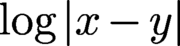 $\log |x - y|$
is a Hilbert–Schmidt operator when
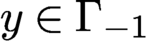 $y \in \Gamma _{-1}$
and
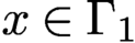 $x \in \Gamma _1$
, it is clear we have
 $$ \begin{align*} {\mathcal L}_{\Gamma_{-1}} |_{\Gamma_{1}} w_{-1} \boldsymbol{T}_{-1} = \boldsymbol{T}_1 L_{T_{-1}}^{T_1}, \end{align*} $$
where
 $L_{T_{-1}}^{T_1}$
is a compact operator in appropriate spaces (in fact, any algebraically decaying space). Thus we can effectively approximate it by a finite-dimensional matrix
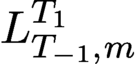 $L_{T_{-1},m}^{T_1}$
. The entries can be calculated via a variety of means such as a tensor product constructors or exploiting the recurrence relationship. Here we use the following approximation:
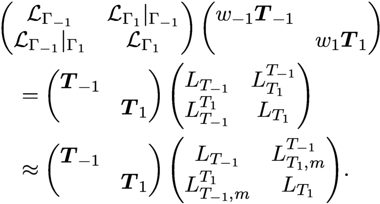 $$ \begin{align*} & \begin{pmatrix} {\mathcal L}_{\Gamma_{-1}} & {\mathcal L}_{\Gamma_{1}} |_{\Gamma_{-1}} \\ {\mathcal L}_{\Gamma_{-1}} |_{\Gamma_{1}} & {\mathcal L}_{\Gamma_{1}} \end{pmatrix} \begin{pmatrix} w_{-1} \boldsymbol{T}_{-1} & \\ & w_1 \boldsymbol{T}_1\end{pmatrix}\\ &\quad = \begin{pmatrix} \boldsymbol{T}_{-1} & \\ & \boldsymbol{T}_1\end{pmatrix} \begin{pmatrix} L_{T_{-1}} & L_{T_1}^{T_{-1}} \\ L_{T_{-1}}^{T_1} & L_{T_1}\end{pmatrix} \\ &\quad \approx \begin{pmatrix} \boldsymbol{T}_{-1} & \\ & \boldsymbol{T}_1\end{pmatrix} \begin{pmatrix} L_{T_{-1}} & L_{T_1,m}^{T_{-1}} \\ L_{T_{-1},m}^{T_1} & L_{T_1}\end{pmatrix}\!. \end{align*} $$
The resulting approximation is a finite-dimensional perturbation of a block-diagonal system, and therefore requires only
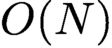 $O({N})$
operations to solve if the right-hand side has N non-zero entries.
The extension to many intervals is also possible. As an example, Figure 7.3(b) shows the acoustic scattering off many metal wires. Note that the complexity does depend on the geometry: the closer the intervals are to each other the larger m must be, and the total perturbation from diagonal typically grows with the number of intervals. Hierarchical matrix methods may provide an attractive way around this issue.
7.6 Other geometries
It is also possible to calculate Cauchy transforms over smooth arcs by approximating them using a degree d polynomial map
 $p \colon [-1,1] \rightarrow \Gamma $
, which is one-to-one. By using an explicit change-of-variable formula found in Olver (Reference Olver2012) and Trogdon and Olver (Reference Trogdon and Olver2016), we have
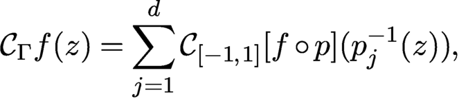 $$ \begin{align*} {\mathcal C}_\Gamma f(z) = \sum_{j=1}^d {\mathcal C}_{[-1,1]}[f \circ p](p_j^{-1}(z)), \end{align*} $$
where
 $p_1^{-1}(z), \ldots , p_d^{-1}(z)$
are the d pre-images of p. That is,
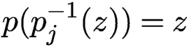 $p(p_j^{-1}(z)) = z$
. This leads to an expression
 $$ \begin{align*} {\mathcal H}_\Gamma f(s) = {\mathcal H}_{[-1,1]}[f \circ p](p^{-1}(s)) + \text{compact}, \end{align*} $$
where
 $p^{-1} \colon \Gamma \rightarrow [-1,1]$
. This shows that the ultraspherical spectral method for SIEs extends naturally to the mapped basis
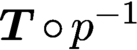 $\boldsymbol {T} \circ p^{-1}$
:
 $$ \begin{align*} {\mathcal H}_\Gamma (\boldsymbol{T} \circ p^{-1}) =( \boldsymbol{U} \circ p^{-1}) [H_T^U + \text{compact}]. \end{align*} $$
The log kernel can be handled similarly using the expressionFootnote 12
 $$ \begin{align*} {\mathcal L}_\Gamma f(z) = \sum_{j=1}^d {\mathcal L}_{[-1,1]} \{(f \circ p) {|p'|}\}{(p_j^{-1}(z))} + \log M \int_\Gamma f {\mathrm{d}} s, \end{align*} $$
where
 $p(z) = M z^d + O({z^{d-1}})$
. What remains unclear is how to handle geometries with corners.
7.7 Fractional differential equations
Orthogonal polynomials have nice recurrence relationships for fractional derivatives, which have been used in the construction of collocation schemes (Zayernouri and Karniadakis Reference Zayernouri and Karniadakis2014, Chen, Shen and Wang Reference Chen, Shen and Wang2016), achieving spectral accuracy when the solution is smooth. Hale and Olver (Reference Hale and Olver2018) considered equations involving one-sided fractional integral operators and fractional differential equations of Riemann–Liouville or Caputo type of rational order. This has the interesting feature of considering an expansion in multiple types of singularities at the same time; for example, the solution looks like
 $$ \begin{align*} u(x) = f(x) + \sqrt{x} g(x), \end{align*} $$
where f and g are smooth, and the approximation is achieved using suitably chosen orthogonal expansion bases. Extensions to fractional Laplacians also appear to be feasible. For brevity we refer the readers to the existing publications, but please stay tuned to new publications as this is evolving rapidly.
On the sphere, fractional differential operators have representations in terms of spherical harmonic expansions, which have been successfully used in combination with fast spherical harmonic transforms (Slevinsky, Montanelli and Du Reference Slevinsky, Montanelli and Du2018) to compute solutions to fractional evolution equations.
8 Conclusions
Despite over a hundred years of research, there are many directions for future work on OPs.
-
(1) Semiclassical orthogonal polynomials. These are becoming increasingly of interest in applications to frames (Huybrechs Reference Huybrechs2010), computations on geometries defined by quadratic curves (Olver and Xu Reference Olver and Xu2019b , Olver and Xu Reference Olver and Xu2020b , Olver and Xu Reference Olver and Xu2020a ) including solving PDEs on light cones (Olver and Xu Reference Olver and Xu2019a ) and disk slices and trapeziums (Snowball and Olver Reference Snowball and Olver2020). We anticipate that semiclassical OPs will become increasingly important in applications involving non-standard geometries.
-
(2) Multivariate orthogonal polynomials that are not constructed by tensorization or by Koornwinder’s method (which implies they are separable in some coordinate system). This makes transforms much more expensive as even direct non-separable transforms in d dimensions cost
${O} (N^{2d})$
for
$N^d$
degrees of freedom. With separability in all d dimensions, the direct cost is only
${O} (N^{d+1})$
. -
(3) Full
$hp$
-adaptivity in spectral element methods. For small p, effective h adaptivity is prevalent and effective (Karniadakis and Sherwin Reference Karniadakis and Sherwin2013). In this review we have focused on large p, where sparsity in the discretization lends itself to effective p-adaptive schemes. What remains open is how to synthesize the two regimes effectively. -
(4) Eigenproblems with continuous spectra. Orthogonal polynomials simultaneously solve differential eigenvalue problems with discrete spectra and are eigenfunctions of Jacobi operators with continuous spectra. This hints at the possibility of their use in solving differential equations with continuous spectra without discretizing the spectrum itself. Promising work along this avenue includes that of Webb (Reference Webb2017).
-
(5) Spectral methods for non-local analogues of calculus operators (Du, Gunzburger, Lehoucq and Zhou Reference Du, Gunzburger, Lehoucq and Zhou2012, Du, Gunzburger, Lehoucq and Zhou Reference Du, Gunzburger, Lehoucq and Zhou2013).
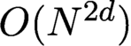

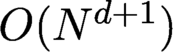

A Classical orthogonal polynomial recurrencerelationships
A.1 Jacobi
The results in this appendix hold when
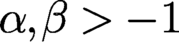 $\alpha ,\beta>-1$
. Throughout this appendix, ‘DLMF’ refers to the NIST Handbook of Mathematical Functions (Olver, Lozier, Boisvert and Clark Reference Olver, Lozier, Boisvert and Clark2010).
Proposition A.1 (mass matrix (DLMF, Table 18.3.1)).
We have
 $$ \begin{align*} ({\boldsymbol{P}}^{(\alpha,\beta)})^{\top} (1-x)^\alpha (1+x)^\beta {\boldsymbol{P}}^{(\alpha,\beta)} = M_{(\alpha,\beta)}, \end{align*} $$
where
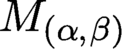 $M_{(\alpha ,\beta )}$
is the diagonal matrix satisfying
 $$ \begin{align*} (M_{(\alpha,\beta)})_{n,n} = 2^{\alpha + \beta + 1} \displaystyle \frac{\Gamma(n+\alpha+1) \Gamma(n+\beta+1) }{ (2n+\alpha+\beta+1) \Gamma(n+\alpha+\beta+1) n!}. \end{align*} $$
Proposition A.2 (reflection).
For the reflection operator
 $$ \begin{align*} {\mathcal R}f(x) := f(-x) {,} \end{align*} $$
we have
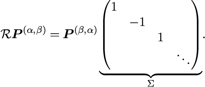 $$ \begin{align*} {\mathcal R} {\boldsymbol{P}}^{(\alpha,\beta)} = {\boldsymbol{P}}^{(\beta,\alpha)} \underbrace{\begin{pmatrix} 1 \\ & -1 \\ && 1 \\ &&&\ddots \end{pmatrix}}_{\Sigma}\!. \end{align*} $$
Proposition A.3 (conversion (DLMF, 18.9.5)).
For Jacobi polynomials the conversion is given by
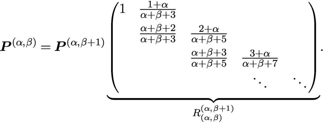 $$ \begin{align*} {\boldsymbol{P}}^{(\alpha,\beta)} = {\boldsymbol{P}}^{(\alpha,\beta+1)} \underbrace{\begin{pmatrix} 1 & \frac{1+\alpha}{\alpha+\beta+3} & & \\[5pt] & \frac{\alpha+\beta+2}{\alpha+\beta+3} & \frac{2+\alpha}{\alpha+\beta+5} & \\[5pt] & & \frac{\alpha+\beta+3}{\alpha+\beta+5} & \frac{3+\alpha}{\alpha+\beta+7} \\ &&& \ddots & \ddots \end{pmatrix}}_{R_{(\alpha,\beta)}^{(\alpha,\beta+1)}}\!. \end{align*} $$
We also have
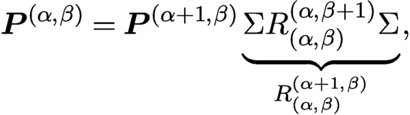 $$ \begin{align*} {\boldsymbol{P}}^{(\alpha,\beta)} = {\boldsymbol{P}}^{(\alpha+1,\beta)} \underbrace{ \Sigma R_{(\alpha,\beta)}^{(\alpha,\beta+1)} \Sigma}_{R_{(\alpha,\beta)}^{(\alpha+1,\beta)}}, \end{align*} $$
where
 $\Sigma $
was defined in Proposition A.2. The conversion operator
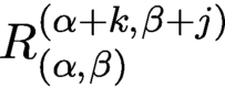 $R_{(\alpha ,\beta )}^{(\alpha +k,\beta +j)}$
for integers
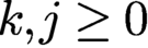 $k,j \geq 0$
can be defined by composing conversions together; for example,
 $$ \begin{align*} {R_{(\alpha,\beta)}^{(\alpha+k,\beta+j)} := R_{(\alpha+k,\beta+j-1)}^{(\alpha+k,\beta+j)} \cdots R_{(\alpha+k,\beta)}^{(\alpha+k,\beta+1)} R_{(\alpha+k-1,\beta)}^{(\alpha+k,\beta)} \cdots R_{(\alpha,\beta)}^{(\alpha+1,\beta)}.} \end{align*} $$
Proposition A.4 (weighted conversion (DLMF, 18.9.5)).
For Jacobi polynomials the weighted conversion is given by
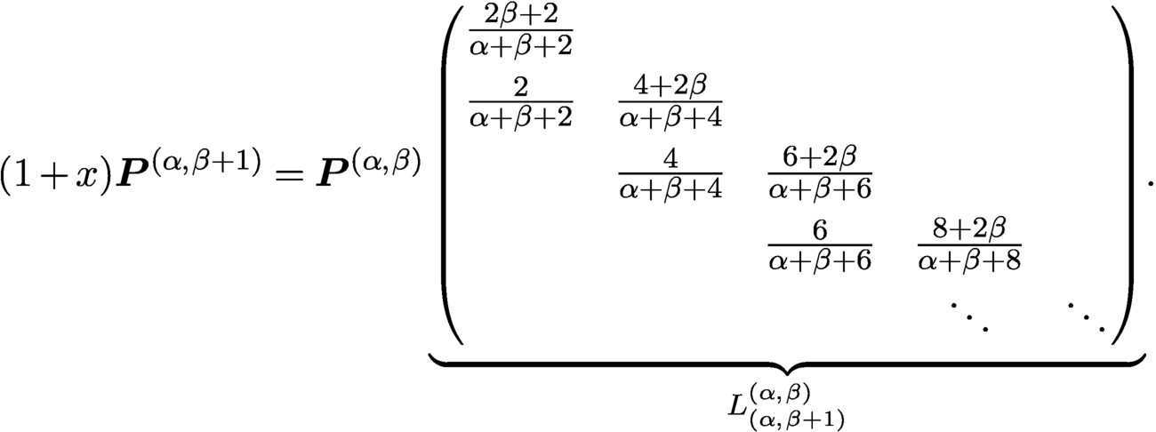 $$ \begin{align*} (1+x) {\boldsymbol{P}}^{(\alpha,\beta+1)} = {\boldsymbol{P}}^{(\alpha,\beta)} \underbrace{\begin{pmatrix} \frac{2\beta+2}{\alpha+\beta+2} & & & \\[5pt] \frac{2}{\alpha+\beta+2} & \frac{4+2\beta}{\alpha+\beta+4} & & \\[5pt] & \frac{4}{\alpha+\beta+4} & \frac{6+2\beta}{\alpha+\beta+6} & \\[5pt] & & \frac{6}{\alpha+\beta+6} & \frac{8+2\beta}{\alpha+\beta+8} \\ &&& \ddots & \ddots \end{pmatrix}}_{L_{(\alpha,\beta+1)}^{(\alpha,\beta)}}\!. \end{align*} $$
We also have
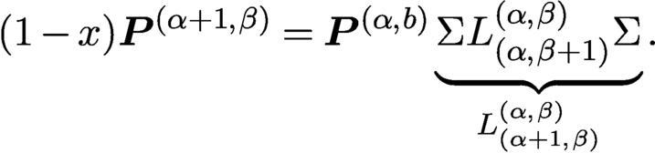 $$ \begin{align*} (1-x) {\boldsymbol{P}}^{(\alpha+1,\beta)} = {\boldsymbol{P}}^{(\alpha,b)} \underbrace{ \Sigma L_{(\alpha,\beta+1)}^{(\alpha,\beta)} \Sigma}_{L_{(\alpha+1,\beta)}^{(\alpha,\beta)}}. \end{align*} $$
The weighted conversion operator
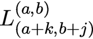 $L_{(a+k,b+j)}^{(a,b)}$
for integers
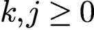 $k,j \geq 0$
can be defined by composing weighted conversions together; for example,
 $$ \begin{align*} L_{(\alpha+k,\beta+j)}^{(\alpha,\beta)} := L_{(\alpha+1,\beta)}^{(\alpha,\beta)} \cdots L_{(\alpha+k,\beta)}^{(\alpha+k-1,\beta)} L_{(\alpha+k,\beta+1)}^{(\alpha+k,\beta)} \cdots L_{(\alpha+k,\beta+j)}^{(\alpha+k,\beta+j-1)}. \end{align*} $$
Proposition A.5 (differentiation (DLMF, 18.9.15)).
For the derivative operator
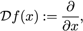 $$ \begin{align*}{\mathcal D} f (x) :=\displaystyle \frac{\partial }{ \partial x} {,} \end{align*} $$
we have
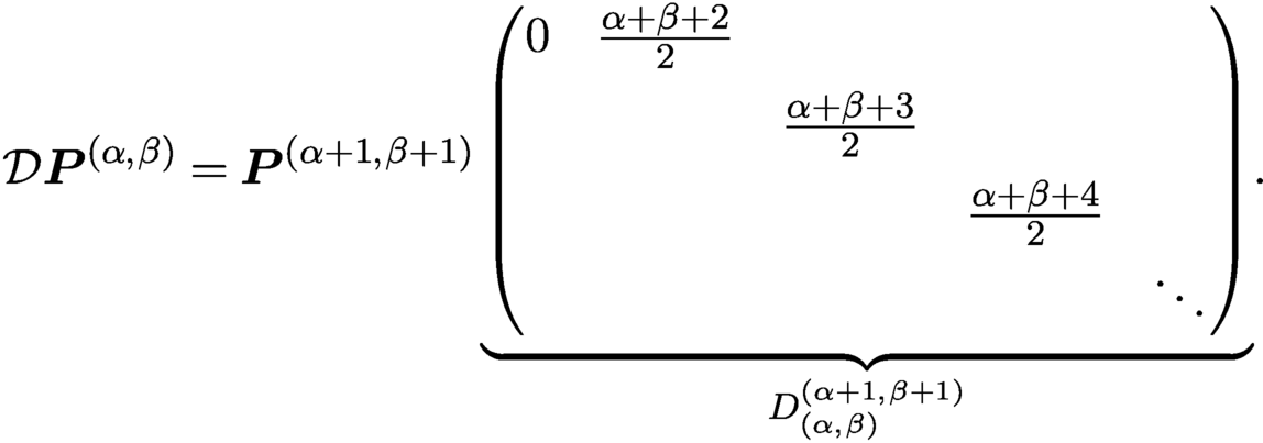 $$ \begin{align*} {\mathcal D} {\boldsymbol{P}}^{(\alpha,\beta)} = {\boldsymbol{P}}^{(\alpha+1,\beta+1)} \underbrace{\begin{pmatrix} 0 & \frac{\alpha+\beta+2}{2} & & \\[5pt] & & \frac{\alpha+\beta+3}{2} & \\[5pt] & & & \frac{\alpha+\beta+4}{2} \\ & & & & \ddots \end{pmatrix}}_{D_{(\alpha,\beta)}^{(\alpha+1,\beta+1)}}\!. \end{align*} $$
Proposition A.6 (weighted differentiation (DLMF, 18.9.16)).
The weighted differentiation operator is given by
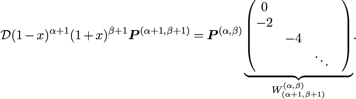 $$ \begin{align*} {\mathcal D} (1-x)^{\alpha+1} (1+x)^{\beta+1} \boldsymbol{P}^{(\alpha+1,\beta+1)} = \boldsymbol{P}^{(\alpha,\beta)} \underbrace{\begin{pmatrix} 0 \\ -2 \\ & -4 \\ && \ddots & \end{pmatrix}}_{W_{(\alpha+1,\beta+1)}^{(\alpha,\beta)}}\!. \end{align*} $$
Proposition A.7 (one-sided weighted differentiation.).
The one-sided weighted differentiation operators are given by
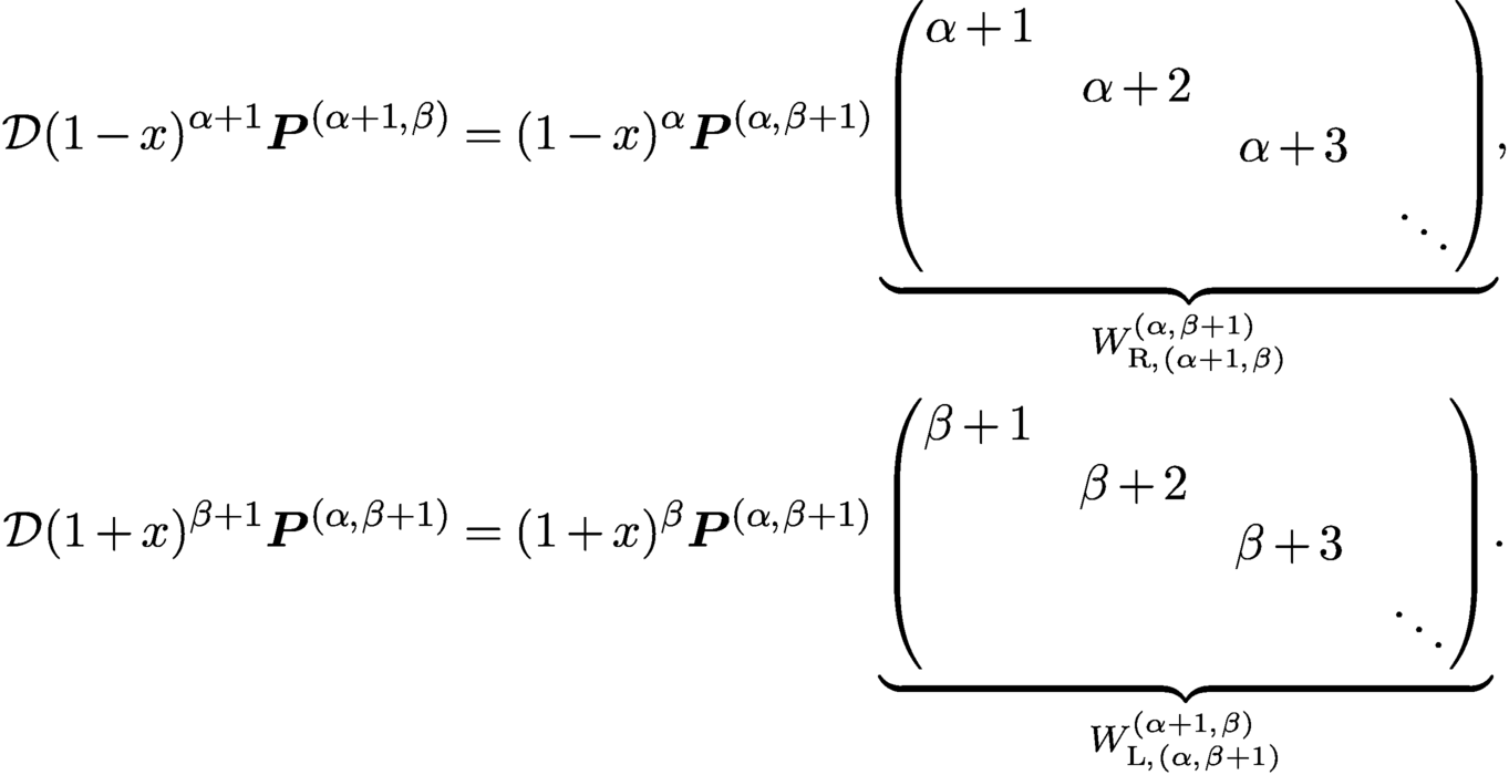 $$ \begin{align*} {\mathcal D} (1-x)^{\alpha+1} \boldsymbol{P}^{(\alpha+1,\beta)} & = (1-x)^{\alpha} \boldsymbol{P}^{(\alpha,\beta+1)} \underbrace{\begin{pmatrix} \alpha+1 \\ & \alpha+2 \\ && \alpha+3 \\ &&& \ddots \end{pmatrix}}_{W_{{\mathrm R},(\alpha+1,\beta)}^{(\alpha,\beta+1)}}\!, \\ {\mathcal D} (1+x)^{\beta+1} \boldsymbol{P}^{(\alpha,\beta+1)} & = (1+x)^\beta \boldsymbol{P}^{(\alpha,\beta+1)} \underbrace{\begin{pmatrix} \beta+1 \\ & \beta+2 \\ && \beta+3 \\ &&& \ddots \end{pmatrix}}_{W_{{\mathrm L},(\alpha,\beta+1)}^{(\alpha+1,\beta)}}\!. \end{align*} $$
Proof. Equivalent to (DLMF, 15.5.4, 15.5.6), as outlined in Olver, Townsend and Vasil (Reference Olver, Townsend and Vasil2020). □
A.2 Ultraspherical
The results in this section hold when
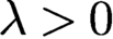 $\lambda>0$
.
Proposition A.8 (mass matrix (DLMF, Table 18.3.1)).
We have
 $$ \begin{align*} (\boldsymbol{C}^{(\lambda)})^{\top} (1-x^2)^{\lambda-1/2} \boldsymbol{C}^{(\lambda)} = M_{(\lambda)}, \end{align*} $$
where
 $M_{(\lambda )}$
is the diagonal matrix satisfying
 $$ \begin{align*} (M_{(\lambda)})_{n,n} = \displaystyle \frac{2^{1-2 \lambda} \pi \Gamma(n+2 \lambda) }{ (n+\lambda) \Gamma(\lambda)^2 n!}. \end{align*} $$
Proposition A.9 (conversion (DLMF, 18.9.7)).
We have
 $$ \begin{align*} \boldsymbol{C}^{(\lambda)} = \boldsymbol{C}^{(\lambda+1)} \underbrace{\begin{pmatrix} 1 & 0 & -\frac{\lambda}{2+\lambda} & \\[5pt] & \frac{\lambda}{1+\lambda} & 0 & -\frac{\lambda}{3+\lambda} \\[5pt] & & \frac{\lambda}{2+\lambda} & 0 & -\frac{\lambda}{5+\lambda} \\ & & & \ddots & \ddots & \ddots \end{pmatrix} }_{R_{(\lambda)}^{(\lambda+1)}} \end{align*} $$
for the conversion between ultraspherical polynomials. By composing conversions, we have
 $R_{(\lambda )}^{(\lambda +m)} = R_{(\lambda +m-1)}^{(\lambda +m)} \cdots R_{(\lambda )}^{(\lambda +1)}$
.
Proposition A.10 (weighted conversion (DLMF, 18.9.8)).
We have
 $$ \begin{align*} (1-x^2) \boldsymbol{C}^{(\lambda+1)} = \boldsymbol{C}^{(\lambda)}L_{(\lambda+1)}^{(\lambda)}, \end{align*} $$
for the weighted conversion between ultraspherical polynomials, where the entries of
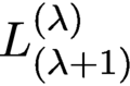 $L_{(\lambda +1)}^{(\lambda )}$
are determined by the recurrence
 $$ \begin{align*} & 4\lambda(n+\lambda+1)(1-x^{2})C^{(\lambda+1)}_{n}(x)\\ &\quad =-(n+1)(n+2)C^{ (\lambda)}_{n+2}(x)+(n+2\lambda)(n+2\lambda+1)C^{(\lambda)}_{n} (x). \end{align*} $$
By composing weighted conversions, we have
 $L_{(\lambda +m)}^{(\lambda )} = L_{(\lambda +1)}^{(\lambda )} \cdots L_{(\lambda +m)}^{(\lambda +m-1)}$
.
Proposition A.11 (differentiation (DLMF, 18.9.19)).
For the derivative operator
 ${\mathcal D}$
, we have
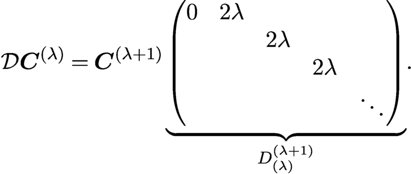 $$ \begin{align*} {\mathcal D} \boldsymbol{C}^{(\lambda)} = \boldsymbol{C}^{(\lambda+1)} \underbrace{\begin{pmatrix}0 & 2\lambda\\ && 2\lambda \\ &&& 2\lambda \\ &&&& \ddots\end{pmatrix}}_{D_{(\lambda)}^{(\lambda+1)}}\!. \end{align*} $$
We also use
 $D_{(\lambda )}^{(\lambda +m)} = D_{(\lambda +m-1)}^{(\lambda +m)} \cdots D_{(\lambda )}^{(\lambda +1)}$
.
A.3 Chebyshev
Proposition A.12 (mass matrix (DLMF, Table 18.3.1)).
We have
 $$ \begin{align*} \boldsymbol{T}^{\top} (1-x^2)^{-1/2} \boldsymbol{T} = M_T, \quad \boldsymbol{U}^{\top} (1-x^2)^{1/2} \boldsymbol{U} = M_U, \end{align*} $$
where
 $M_T$
and
 $M_U$
are diagonal matrices satisfying
 $$ \begin{align*} (M_T)_{0,0} & = \pi , \quad (M_T)_{n,n} = \pi / 2, \quad n> 0, \\ (M_U)_{n,n} & = \pi / 2, \quad n \geq 0. \end{align*} $$
Combining the conversion between Jacobi and Chebyshev/ultraspherical polynomials, we have the following.
Proposition A.13 (conversion (DLMF, 18.9.9, 18.9.11)).
We have
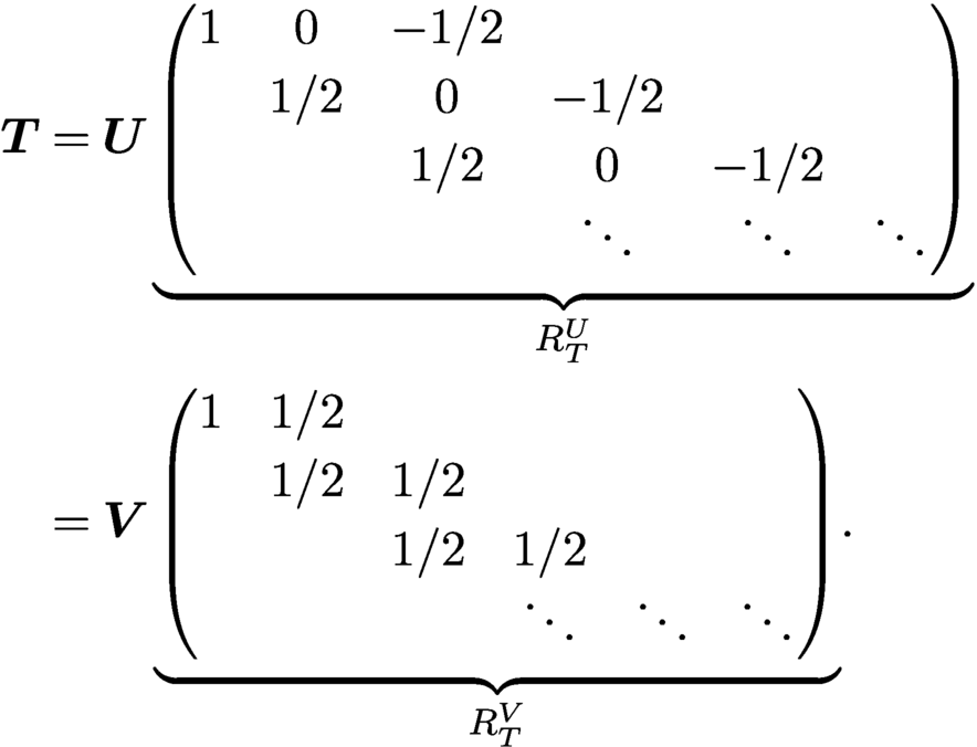 $$ \begin{align*} \boldsymbol{T} & = \boldsymbol{U} \underbrace{ \begin{pmatrix} 1 & 0 & -1/2 \\[2pt] & 1/2 & 0 & -1/2 \\[2pt] && 1/2 & 0 & -1/2 \\[-3pt] &&&\ddots & \ddots & \ddots \end{pmatrix}}_{R_T^U}\\ & = \boldsymbol{V} \underbrace{ \begin{pmatrix} 1 & 1/2 \\[2pt] & 1/2 & 1/2 \\[2pt] && 1/2 & 1/2 \\[-3pt] &&&\ddots & \ddots & \ddots \end{pmatrix}}_{R_T^V}\!. \end{align*} $$
We also use
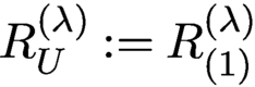 $R_U^{(\lambda )} := R_{(1)}^{(\lambda )}$
and
 $R_T^{(\lambda )} = R_U^{(\lambda )} R_T^U$
.
Proposition A.14 (weighted conversion (DLMF, 18.9.10)).
For the weighted conversion between Chebyshev polynomials we have
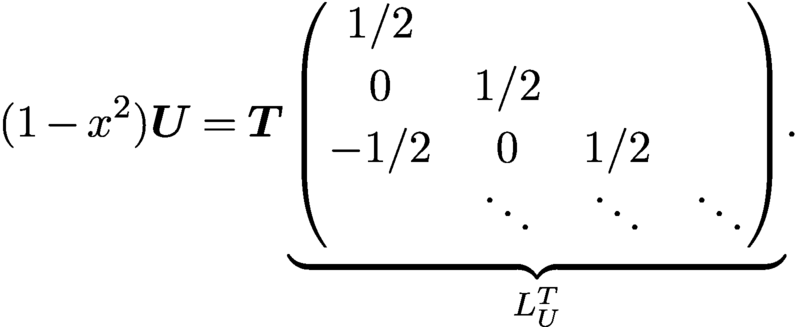 $$ \begin{align*} (1-x^2) \boldsymbol{U} = \boldsymbol{T} \underbrace{ \begin{pmatrix}1/2 \\[2pt] 0 & 1/2 \\[2pt] -1/2 & 0 & 1/2 \\[-3pt] &\ddots & \ddots & \ddots \end{pmatrix}}_{L_U^T}\!. \end{align*} $$
We also have
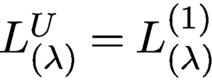 $L_{(\lambda )}^U = L_{(\lambda )}^{(1)}$
and
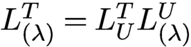 $L_{(\lambda )}^T = L_U^T L_{(\lambda )}^U$
.
Proposition A.15 (differentiation (DLMF, 18.9.21)).
The differentiation operator between Chebyshev polynomials is given by
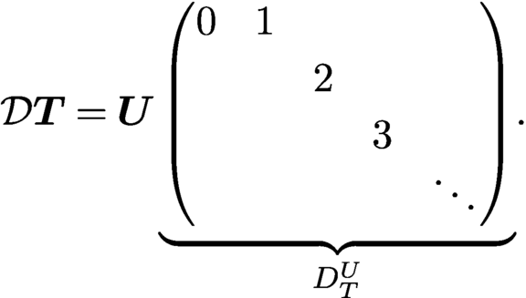 $$ \begin{align*} {\mathcal D} \boldsymbol{T} = \boldsymbol{U} \underbrace{\begin{pmatrix}0 & 1 \\[2pt] && 2 \\[2pt] &&& 3 \\[-3pt] &&&& \ddots\end{pmatrix}}_{D_T^U}\!. \end{align*} $$
We also have
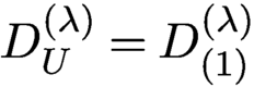 $D_U^{(\lambda )} = D_{(1)}^{(\lambda )}$
and
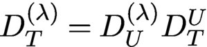 $D_T^{(\lambda )} = D_U^{(\lambda )} D_T^U$
.
Proposition A.16 (weighted differentiation (DLMF, 18.9.22)).
The weighted differentiation operator for Chebyshev polynomials is givenby
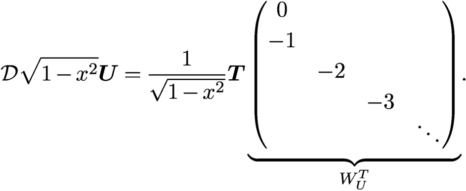 $$ \begin{align*} {\mathcal D} \sqrt{1-x^2} \boldsymbol{U} = \displaystyle \frac{1 }{ \sqrt{1-x^2}} \boldsymbol{T} \underbrace{\begin{pmatrix}0\\[2pt] -1 \\[2pt] & -2 \\[2pt] && -3 \\[-3pt] &&& \ddots\end{pmatrix}}_{W_U^T}\!. \end{align*} $$
We also have
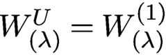 $W_{(\lambda )}^U = W_{(\lambda )}^{(1)}$
and
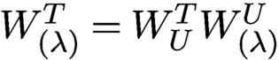 $W_{(\lambda )}^T = W_U^T W_{(\lambda )}^U$
.
Proposition A.17 (integration).
Let
 ${\mathcal Q}$
denote the indefinite integration operator normalized so that the zeroth Chebyshev coefficient vanishes. That is,
 $$ \begin{align*} {\mathcal D}{\mathcal{Q}} = {\mathcal I},\quad \int_{-1}^1 \displaystyle \frac{({\mathcal Q} f)(x) }{ \sqrt{1-x^2}} {{\mathrm{d}}x} = 0. \end{align*} $$
Then we have
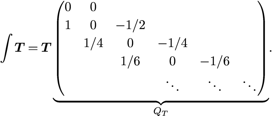 $$ \begin{align*} \int \boldsymbol{T} = \boldsymbol{T} \underbrace{\begin{pmatrix} 0 & 0 \\[2pt] 1 & 0 & -1/2 \\[2pt] & 1/4 & 0 & -1/4 \\[2pt] && 1/6 & 0 & -1/6 \\[2pt] & & & \ddots & \ddots & \ddots \end{pmatrix} }_{Q_T}\!. \end{align*} $$
Proof. This follows from the relation
 $$ \begin{align*} {\mathcal{Q}} \boldsymbol{T} Q_T = \boldsymbol{U} D_T^U Q_T {,} \end{align*} $$
and observing that
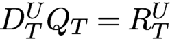 $D_T^U Q_T = R_T^U$
.□
A.4 Laguerre
We use a tilde above operators for Laguerre polynomials to avoid confusion with ultraspherical polynomials. The results in this section hold when
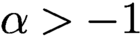 ${\alpha>-1}$
.
Proposition A.18 (mass matrix (DLMF, Table 18.3.1)).
We have
 $$ \begin{align*} (\boldsymbol{L}^{(\alpha)})^{\top} x^\alpha \,{\mathrm{e}}^{-x} \boldsymbol{L}^{(\alpha)} = \tilde M_{(\alpha)}, \end{align*} $$
where
 $\tilde M_{(\alpha )}$
is the diagonal matrix satisfying
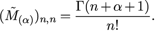 $$ \begin{align*} (\tilde M_{(\alpha)})_{n,n} = \displaystyle \frac{\Gamma(n+\alpha+1) }{ n!}. \end{align*} $$
Proposition A.19 (conversion).
We have
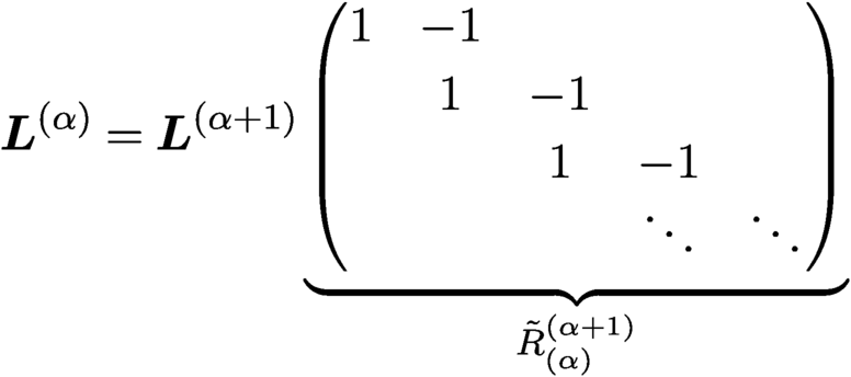 $$ \begin{align*} \boldsymbol{L}^{(\alpha)} = \boldsymbol{L}^{(\alpha+1)} \underbrace{\begin{pmatrix} 1 & -1 \\[2pt] & 1 & -1 \\[2pt] & & 1 & -1 \\[-3pt] & & & \ddots & \ddots \end{pmatrix} }_{\tilde R_{(\alpha)}^{(\alpha+1)}} \end{align*} $$
for the conversion operator between Laguerre polynomials. We also have
 $\tilde R_{(\alpha )}^{(\alpha +m)} = \tilde R_{(\alpha +m-1)}^{(\alpha +m)} \cdots \tilde R_{(\alpha )}^{(\alpha +1)}$
.
Proposition A.20 (weighted conversion).
For the weighted conversion operator we have
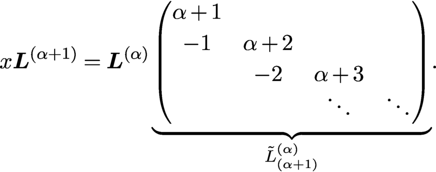 $$ \begin{align*} x \boldsymbol{L}^{(\alpha+1)} = \boldsymbol{L}^{(\alpha)} \underbrace{\begin{pmatrix} \alpha+1 \\[2pt] -1 & \alpha+2 \\[2pt] &-2 & \alpha+3 \\[-3pt] &&\ddots & \ddots \end{pmatrix} }_{\tilde L_{(\alpha+1)}^{(\alpha)}}\!. \end{align*} $$
We also have
 $\tilde L_{(\alpha +m)}^{(\alpha )} = \tilde L_{(\alpha +1)}^{(\alpha )} \cdots \tilde L_{(\alpha +m)}^{(\alpha +m-1)}$
.
Proposition A.21 (differentiation (DLMF, 18.9.23)).
The differentiation operator for Laguerre is given by
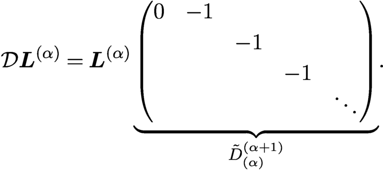 $$ \begin{align*} {\mathcal D} \boldsymbol{L}^{(\alpha)} = \boldsymbol{L}^{(\alpha)} \underbrace{\begin{pmatrix}0 & -1 \\[2pt] && -1 \\[2pt] &&& -1 \\[-3pt] &&&& \ddots\end{pmatrix}}_{\tilde D_{(\alpha)}^{(\alpha+1)}}\!. \end{align*} $$
Proposition A.22 (weighted differentiation (DLMF, 18.9.24)).
The weighted differentiation operator for Laguerre is given by
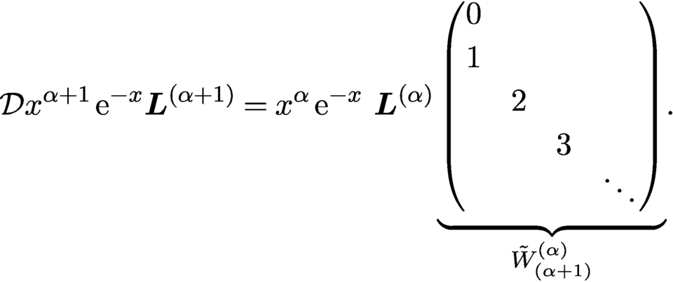 $$ \begin{align*} {\mathcal D} x^{\alpha+1} \,{\mathrm{e}}^{-x} \boldsymbol{L}^{(\alpha+1)} =x^{\alpha} \,{\mathrm{e}}^{-x} \ \boldsymbol{L}^{(\alpha)} \underbrace{\begin{pmatrix}0 \\[2pt] 1 \\[2pt] & 2 \\[2pt] && 3 \\[-3pt] &&& \ddots\end{pmatrix}}_{\tilde W_{(\alpha+1)}^{(\alpha)}}\!. \end{align*} $$
A.5 Hermite
Proposition A.23 (mass matrix (DLMF, Table 18.3.1)).
We have
 $$ \begin{align*} \boldsymbol{H} ^{\top} \,{\mathrm{e}}^{-x^2} \boldsymbol{H} = M_H, \end{align*} $$
where
 $M_H$
is the diagonal matrix satisfying
 $(M_H)_{n,n} =\sqrt {\pi } 2^n n!$
.
Proposition A.24 (differentiation (DLMF, 18.9.25)).
The differentiation operator for Hermite is given by
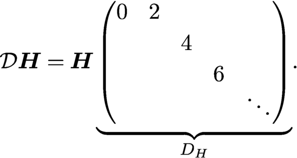 $$ \begin{align*} {\mathcal D} \boldsymbol{H} = \boldsymbol{H} \underbrace{\begin{pmatrix}0 & 2 \\[2pt] && 4 \\[2pt] &&& 6 \\[-3pt] &&&& \ddots\end{pmatrix}}_{D_H}\!. \end{align*} $$
Proposition A.25 (weighted differentiation (DLMF, 18.9.26)).
The weighted differentiation operator for Hermite is given by
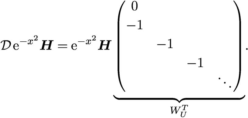 $$ \begin{align*} {\mathcal D} \,{\mathrm{e}}^{-x^2} \boldsymbol{H} = {\mathrm{e}}^{-x^2} \boldsymbol{H} \underbrace{\begin{pmatrix}0\\[2pt] -1 \\[2pt] & -1 \\[2pt] && -1 \\[-3pt] &&& \ddots\end{pmatrix}}_{W_U^T}\!. \end{align*} $$
A.6 Associated Legendre polynomials
The associated Legendre polynomials satisfy the relationship
 $$ \begin{align*} P_n^m(x) = ({1 / 2})_m (-2)^m (1-x^2)^{m/2} C_{n-m}^{(m+1/2)}(x) \end{align*} $$
or, in quasimatrix notation, we have
 $$ \begin{align*} \boldsymbol{P}^m = ({1 / 2})_m (-2)^m (1-x^2)^{m/2} \boldsymbol{C}^{(m+1/2)}. \end{align*} $$
We thus inherit the recurrence relationships from the ultraspherical polynomials; for example,
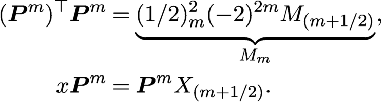 $$ \begin{align} (\boldsymbol{P}^m)^{\top} \boldsymbol{P}^m &= \underbrace{({1 / 2})_m^2 (-2)^{2m} M_{(m+1/2)}}_{M_m}, \notag \\ x \boldsymbol{P}^m &= \boldsymbol{P}^m X_{(m+1/2)}. \end{align} $$
B Multivariate orthogonal polynomial and their recurrence relationships
B.1 Jacobi polynomials on the triangle
Here, we outline the recurrence relationships for
 $$ \begin{align*} P_{n,k}^{(a,b,c)}(x,y) := P_{n-k}^{(2k+b+c+1,a)}(2x-1) (1-x)^k P_k^{(c,b)}\biggl(\displaystyle \frac{2y }{ 1-x}-1\biggr), \end{align*} $$
which are derived by Xu (Reference Xu2017) and Olver et al. (Reference Olver, Townsend and Vasil2020). Here,
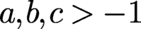 $a,b,c>-1$
and
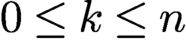 $0\leq k\leq n$
. We define
 $z := 1-x-y$
and
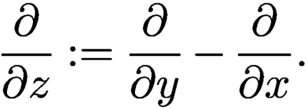 $$ \begin{align*} \displaystyle \frac{\partial }{ \partial z} := \displaystyle \frac{\partial }{ \partial y} - \displaystyle \frac{\partial }{ \partial x}.\end{align*} $$
Proposition B.1 (mass matrix (Dunkl and Xu Reference Dunkl and Xu2014)).
We have
 $$ \begin{align*} (\boldsymbol{P}^{(a,b,c)})^{\top} x^a y^b z^c \boldsymbol{P}^{(a,b,c)} = M_{(a,b,c)}, \end{align*} $$
where
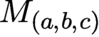 $M_{(a,b,c)}$
is a diagonal matrix whose diagonal is a block-vector. The kth entry of the nth block is given by
 $$ \begin{align*} & \displaystyle \frac{1 }{ 2^{2k+a+2b+2c+3}} (M_{(2k+b+c+1,a)})_{n-k,n-k} (M_{(c,b)})_{k,k} \\ & \! = \! \displaystyle\frac{\Gamma(n+k+b+c+2) \Gamma(n-k+a+1) \Gamma(k+b+1) \Gamma(k+c+1) }{(2n+a+b+c+2) (2k+b+c+1) \Gamma(n+k+a+b+c+2)\Gamma(k+b+c+1) (n-k)! k!}. \end{align*} $$
Corollary B.2 (Olver et al. Reference Olver, Townsend and Vasil2020, Corollary 1).
The following recurrence relations for the partial derivatives hold:
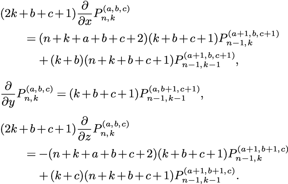 $$ \begin{align*} & \begin{aligned} & (2k+b+c+1) \displaystyle \frac{\partial }{ \partial x} P_{n,k}^{(a,b,c)} \\ & \qquad = (n+k+a+b+c+2)(k+b+c+1){P}_{n-1,k}^{(a+1,b,c+1)} \notag\\ & \qquad\quad\, + (k+b)(n+k+b+c+1){P}_{n-1,k-1}^{(a+1,b,c+1)}, \end{aligned}\\[6pt] & \displaystyle \frac{\partial }{ \partial y} P_{n,k}^{(a,b,c)} = (k + b + c + 1) {P}_{n-1,k-1}^{(a,b+1,c+1)},\\[3pt] &\begin{aligned} &(2k+b+c+1){\displaystyle \frac{\partial }{ \partial z}} P_{n,k}^{(a,b,c)} \\ & \qquad = -(n+k+a+b+c+2) (k+b+c+1) {P}_{n-1,k}^{(a+1,b+1,c)} \notag \\ &\qquad\quad\, + (k+c)(n+k+b+c+1) {P}_{n-1,k-1}^{(a+1,b+1,c)}. \end{aligned}\\[-20pt] \end{align*} $$
They give the entries of sparse matrices satisfying
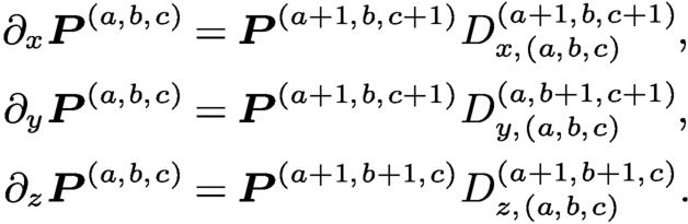 $$ \begin{align*} \partial_x \boldsymbol{P}^{(a,b,c)} & = \boldsymbol{P}^{(a+1,b,c+1)} D_{x,(a,b,c)}^{(a+1,b,c+1)}, \\[0pt] \partial_y \boldsymbol{P}^{(a,b,c)} & = \boldsymbol{P}^{(a+1,b,c+1)} D_{y,(a,b,c)}^{(a,b+1,c+1)}, \\[0pt] \partial_z \boldsymbol{P}^{(a,b,c)} & = \boldsymbol{P}^{(a+1,b+1,c)} D_{z,(a,b,c)}^{(a+1,b+1,c)}. \end{align*} $$
Each matrix is block-super-diagonal with diagonal (
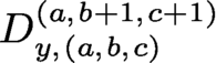 $D_{y,(a,b,c)}^{(a,b+1,c+1)}$
) or upper-bidiagonal (
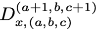 $D_{x,(a,b,c)}^{(a+1,b,c+1)}$
and
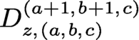 $ D_{z,(a,b,c)}^{(a+1,b+1,c)}$
) blocks.
Corollary B.3 (Olver et al. Reference Olver, Townsend and Vasil2020, Corollary 2).
The following recurrence relations for the weighted partial derivatives hold:
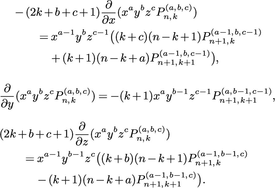 $$ \begin{align*} &\begin{aligned} & -(2k+b+c+1)\displaystyle \frac{\partial }{ \partial x} (x^a y^b z^c P_{n,k}^{(a,b,c)}) \\ & \qquad = x^{a-1}y^b z^{c-1}\big( (k+c)(n-k+1){P}_{n+1,k}^{(a-1,b,c-1)} \\ &\qquad\quad\, + (k+1)(n-k+a){P}_{n+1,k+1}^{(a-1,b,c-1)}\big), \end{aligned}\end{align*}\begin{align*}& \displaystyle \frac{\partial }{ \partial y}(x^a y^b z^c P_{n,k}^{(a,b,c)}) = -(k+1)x^ay^{b-1} z^{c-1} {P}_{n+1,k+1}^{(a,b-1,c-1)},\\[6pt] &\begin{aligned} &(2k+b+c+1) {\displaystyle \frac{\partial }{ \partial z}} (x^a y^b z^c P_{n,k}^{(a,b,c)}) \\ &\qquad = x^{a-1}y^{b-1} z^c \big((k+b)(n-k+1){P}_{n+1,k}^{(a-1,b-1,c)} \\ &\qquad\quad\, - (k+1)(n-k+a){P}_{n+1,k+1}^{(a-1,b-1,c)}\big). \end{aligned} \end{align*} $$
They give the entries of sparse matrices satisfying
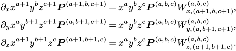 $$ \begin{align*} {\partial_x} x^{a+1} y^b z^{c+1} \boldsymbol{P}^{(a+1,b,c+1)} & = x^a y^b z^c \boldsymbol{P}^{(a,b,c)} W_{x,(a+1,b,c+1)}^{(a,b,c)}, \\ {\partial_y} x^{a} y^{b+1} z^{c+1} \boldsymbol{P}^{(a,b+1,c+1)} & = x^a y^b z^c \boldsymbol{P}^{(a,b,c)} W_{y,(a,b+1,c+1)}^{(a,b,c)}, \\ {\partial_z} x^{a+1} y^{b+1} z^{c} \boldsymbol{P}^{(a+1,b+1,c)} & = x^a y^b z^c \boldsymbol{P}^{(a,b,c)} W_{z,(a+1,b+1,c)}^{(a,b,c)}. \end{align*} $$
Each matrix is block-sub-diagonal with diagonal (
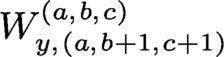 $W_{y,(a,b+1,c+1)}^{(a,b,c)}$
) or lower-bidiagonal (
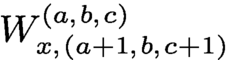 $W_{x,(a+1,b,c+1)}^{(a,b,c)}$
and
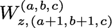 $W_{z,(a+1,b+1,c)}^{(a,b,c)}$
) blocks.
Corollary B.4 (Olver et al. Reference Olver, Townsend and Vasil2020, Corollary 3).
The following recurrence relations for conversions hold:
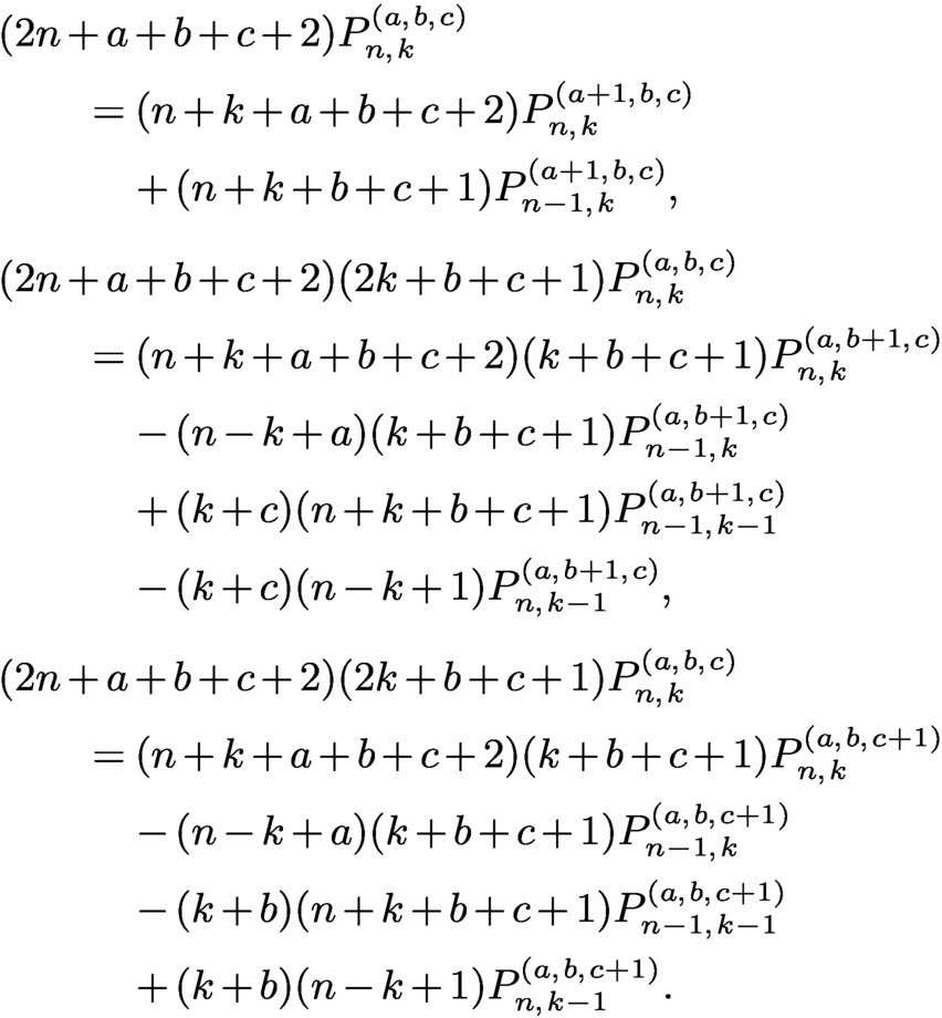 $$ \begin{align*} &\begin{aligned} & (2n+a+b+c+2)P_{n,k}^{(a,b,c)} \\ &\qquad = (n+k+a+b+c+2){P}_{n,k}^{(a+1,b,c)} \\ & \qquad\quad\, + (n+k+b+c+1){P}_{n-1,k}^{(a+1,b,c)}, \end{aligned}\\[3pt] & \begin{aligned} &(2n+a+b+c+2)(2k+b+c+1)P_{n,k}^{(a,b,c)}\\ & \qquad = (n+k+a+b+c+2)(k+b+c+1){P}_{n,k}^{(a,b+1,c)} \\ &\qquad\quad\, - (n-k+a)(k+b+c+1){P}_{n-1,k}^{(a,b+1,c)}\\ &\qquad\quad\, +(k+c)(n+k+b+c+1){P}_{n-1,k-1}^{(a,b+1,c)}\\ &\qquad\quad\, -(k+c)(n-k+1) {P}_{n,k-1}^{(a,b+1,c)}, \end{aligned}\\[3pt] & \begin{aligned} & (2n+a+b+c+2)(2k+b+c+1)P_{n,k}^{(a,b,c)}\\ &\qquad = (n+k+a+b+c+2)(k+b+c+1){P}_{n,k}^{(a,b,c+1)} \\ &\qquad\quad\, - (n-k+a)(k+b+c+1){P}_{n-1,k}^{(a,b,c+1)}\\ &\qquad\quad\, -(k+b)(n+k+b+c+1){P}_{n-1,k-1}^{(a,b,c+1)}\\ &\qquad\quad\, +(k+b)(n-k+1){P}_{n,k-1}^{(a,b,c+1)}. \end{aligned} \end{align*} $$
They give the entries of sparse matrices satisfying
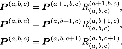 $$ \begin{align*} \boldsymbol{P}^{(a,b,c)} & = \boldsymbol{P}^{(a+1,b,c)} R_{(a,b,c)}^{(a+1,b,c)}, \\ \boldsymbol{P}^{(a,b,c)} & = \boldsymbol{P}^{(a,b+1,c)} R_{(a,b,c)}^{(a,b+1,c)}, \\ \boldsymbol{P}^{(a,b,c)} & = \boldsymbol{P}^{(a,b,c+1)} R_{(a,b,c)}^{(a,b,c+1)}. \end{align*} $$
Each matrix is block-upper-bidiagonal with diagonal (
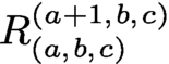 $R_{(a,b,c)}^{(a+1,b,c)}$
) or upper-bidiagonal (
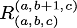 $R_{(a,b,c)}^{(a,b+1,c)}$
and
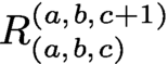 $R_{(a,b,c)}^{(a,b,c+1)}$
) blocks.
Corollary B.5 (Olver et al. Reference Olver, Townsend and Vasil2020, Corollary 4).
The following recurrence relations for lowering operators hold:
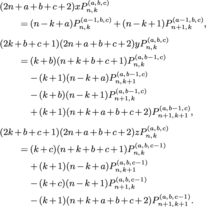 $$ \begin{align*} & \begin{aligned} & (2n+a+b+c+2) x P_{n,k}^{(a,b,c)} \\ &\qquad = (n-k+a) {P}_{n,k}^{(a-1,b,c)} +(n-k+1) {P}_{n+1,k}^{(a-1,b,c)}, \end{aligned}\\[3pt] & \begin{aligned} & (2k+b+c+1)(2n+a+b+c+2) y P_{n,k}^{(a,b,c)}\\ & \qquad = (k+b)(n+k+b+c+1){P}_{n,k}^{(a,b-1,c)}\\ &\qquad\quad\, -(k+1)(n-k+a){P}_{n,k+1}^{(a,b-1,c)}\\ &\qquad\quad\, - (k+b)(n-k+1){P}_{n+1,k}^{(a,b-1,c)}\\ &\qquad\quad\, + (k+1)(n+k+a+b+c+2){P}_{n+1,k+1}^{(a,b-1,c)}, \end{aligned}\\[3pt] & \begin{aligned} & (2 k + b + c+1) (2n + a + b + c + 2)z P_{n,k}^{(a,b,c)} \\ &\qquad = (k + c)(n + k + b + c + 1){P}_{n,k}^{(a,b,c-1)} \\ &\qquad\quad\, + (k + 1)(n - k + a) {P}_{n,k+1}^{(a,b,c-1)}\\ &\qquad\quad\, - (k + c) (n - k + 1){P}_{n+1,k}^{(a,b,c-1)} \\ &\qquad\quad\, - (k + 1)(n + k + a + b + c + 2){P}_{n+1,k+1}^{(a,b,c-1)}. \end{aligned} \end{align*} $$
They give the entries of sparse matrices satisfying
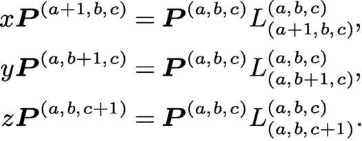 $$ \begin{align*} x \boldsymbol{P}^{(a+1,b,c)} & = \boldsymbol{P}^{(a,b,c)} L_{(a+1,b,c)}^{(a,b,c)}, \\ y \boldsymbol{P}^{(a,b+1,c)} & = \boldsymbol{P}^{(a,b,c)} L_{(a,b+1,c)}^{(a,b,c)}, \\ z \boldsymbol{P}^{(a,b,c+1)} & = \boldsymbol{P}^{(a,b,c)} L_{(a,b,c+1)}^{(a,b,c)}. \end{align*} $$
Each matrix is block-lower-bidiagonal with diagonal (
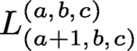 $L_{(a+1,b,c)}^{(a,b,c)}$
) or lower-bidiagonal (
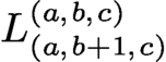 $L_{(a,b+1,c)}^{(a,b,c)}$
and
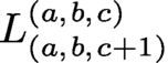 $L_{(a,b,c+1)}^{(a,b,c)}$
) blocks.
B.2 Dirichlet polynomials on the triangle
Imposing Dirichlet conditions requires a special basis, which we denote by
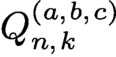 $Q_{n,k}^{(a,b,c)}$
, and forms the quasimatrix
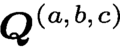 $\boldsymbol {Q}^{(a,b,c)}$
. It is related to negative parameter OPs on the triangle, which are also Sobolev OPs; see Xu (Reference Xu2017). We define
 $\tilde P(x) = P(2x-1)$
to be the shifted Legendre polynomials (Legendre polynomials transplanted onto
 $[0,1]$
.)
Definition B.6. The following polynomials vanish at
 $x = 0$
apart from when
 $k=n$
:
 $$ \begin{align*} Q_{n,k}^{(1,0,0)}(x,y) &:= x P_{n-1,k}^{(1,0,0)}(x,y), \quad 0\leq k \leq n-1, \\ Q_{n,n}^{(1,0,0)}(x,y) &:= P_{n,n}(x,y). \end{align*} $$
The following polynomials vanish at
 $y = 0$
apart from when
 $k=0$
:
 $$ \begin{align*} Q_{n,0}^{(0,1,0)}(x,y) &:= \tilde P_n^{(0,0)}(x), \\ Q_{n,k}^{(0,1,0)}(x,y) &:= y P_{n-1,k-1}^{(0,1,0)}(x,y), \quad 1\leq k\leq n. \end{align*} $$
The following polynomials vanish at
 $z = 0$
(i.e.
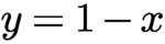 $y = 1-x$
) apart from when
 $k=0$
:
 $$ \begin{align*} Q_{n,0}^{(0,0,1)}(x,y) &:= \tilde P_n^{(0,0)}(x), \\ Q_{n,k}^{(0,0,1)}(x,y) &:= z P_{n-1,k-1}^{(0,0,1)}(x,y), \quad 1\leq k\leq n. \end{align*} $$
The following polynomials vanish at
 $x = 0$
and
 $y = 0$
apart from when
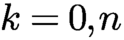 $k = 0, n$
:
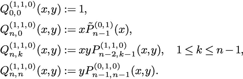 $$ \begin{align*} Q_{0,0}^{(1,1,0)}(x,y) &:= 1, \\ Q_{n,0}^{(1,1,0)}(x,y) &:= x \tilde P_{n-1}^{(0,1)}(x), \\ Q_{n,k}^{(1,1,0)}(x,y) &:= x y P_{n-2,k-1}^{(1,1,0)}(x,y), \quad 1\leq k\leq n-1, \\ Q_{n,n}^{(1,1,0)}(x,y) &:= y P_{n-1,n-1}^{(0,1,0)}(x,y). \end{align*} $$
The following polynomials vanish at
 $x = 0$
and
 $z = 0$
apart from when
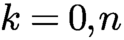 $k = 0, n$
:
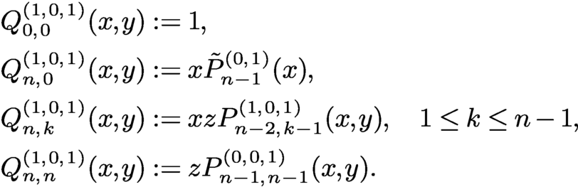 $$ \begin{align*} Q_{0,0}^{(1,0,1)}(x,y) &:= 1, \\ Q_{n,0}^{(1,0,1)}(x,y) &:= x \tilde P_{n-1}^{(0,1)}(x), \\ Q_{n,k}^{(1,0,1)}(x,y) &:= x z P_{n-2,k-1}^{(1,0,1)}(x,y), \quad 1\leq k\leq n-1,\\ Q_{n,n}^{(1,0,1)}(x,y) &:= z P_{n-1,n-1}^{(0,0,1)}(x,y). \end{align*} $$
The following polynomials vanish at
 $y = 0$
and
 $z = 0$
apart from when
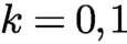 $k = 0, 1$
:
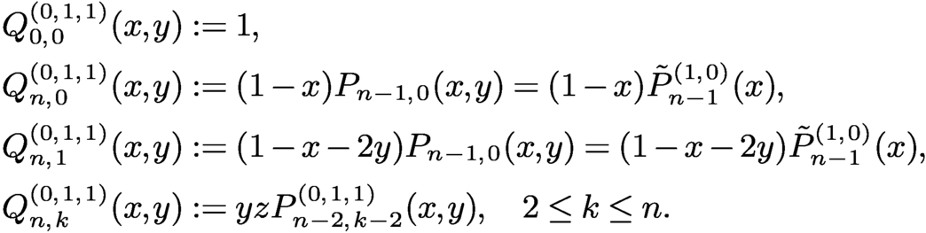 $$ \begin{align*} Q_{0,0}^{(0,1,1)}(x,y) &:= 1, \\ Q_{n,0}^{(0,1,1)}(x,y) &:= (1-x)P_{n-1,0}(x,y) = (1-x)\tilde P_{n-1}^{(1,0)}(x), \\ Q_{n,1}^{(0,1,1)}(x,y) &:= (1-x-2y) P_{n-1,0}(x,y) =(1-x-2y) \tilde P_{n-1}^{(1,0)}(x), \\ Q_{n,k}^{(0,1,1)}(x,y) &:= y z P_{n-2,k-2}^{(0,1,1)}(x,y), \quad 2\leq k\leq n. \end{align*} $$
The following polynomials vanish at
 $x = 0$
,
 $y = 0$
and
 $z = 0$
apart from when
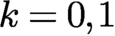 $k = 0,1$
, and
 $ n$
:
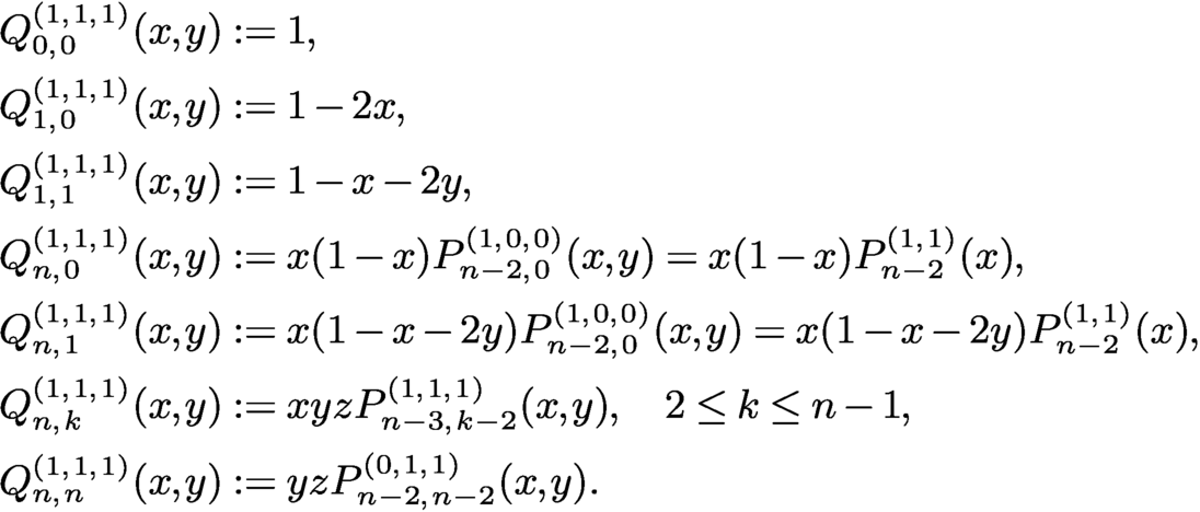 $$ \begin{align*} Q_{0,0}^{(1,1,1)}(x,y) &:= 1, \\ Q_{1,0}^{(1,1,1)}(x,y) &:= 1-2x, \\ Q_{1,1}^{(1,1,1)}(x,y) &:= 1-x-2y, \\ Q_{n,0}^{(1,1,1)}(x,y) &:= x (1-x) P_{n-2,0}^{(1,0,0)}(x,y) = x(1-x) P_{n-2}^{(1,1)}(x), \\ Q_{n,1}^{(1,1,1)}(x,y) &:=x (1-x-2y) P_{n-2,0}^{(1,0,0)}(x,y) = x (1-x-2y) P_{n-2}^{(1,1)}(x), \\ Q_{n,k}^{(1,1,1)}(x,y) &:= x y z P_{n-3,k-2}^{(1,1,1)}(x,y), \quad 2\leq k\leq n-1, \\ Q_{n,n}^{(1,1,1)}(x,y) &:= y z P_{n-2,n-2}^{(0,1,1)}(x,y). \end{align*} $$
Proposition B.7 (conversion (Olver et al. Reference Olver, Townsend and Vasil2019, Corollary C.1–3)).
The following recurrence relationships hold:
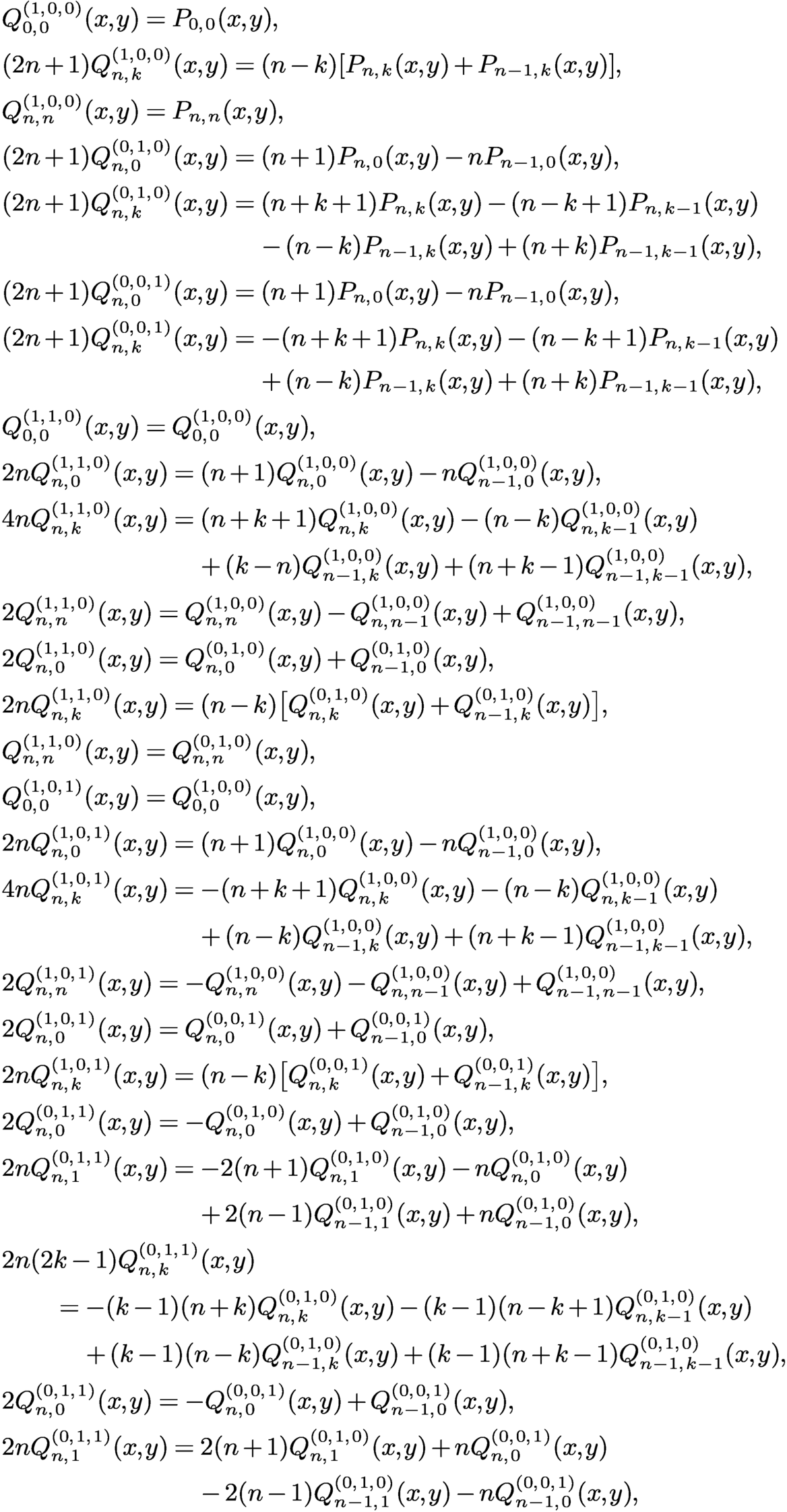
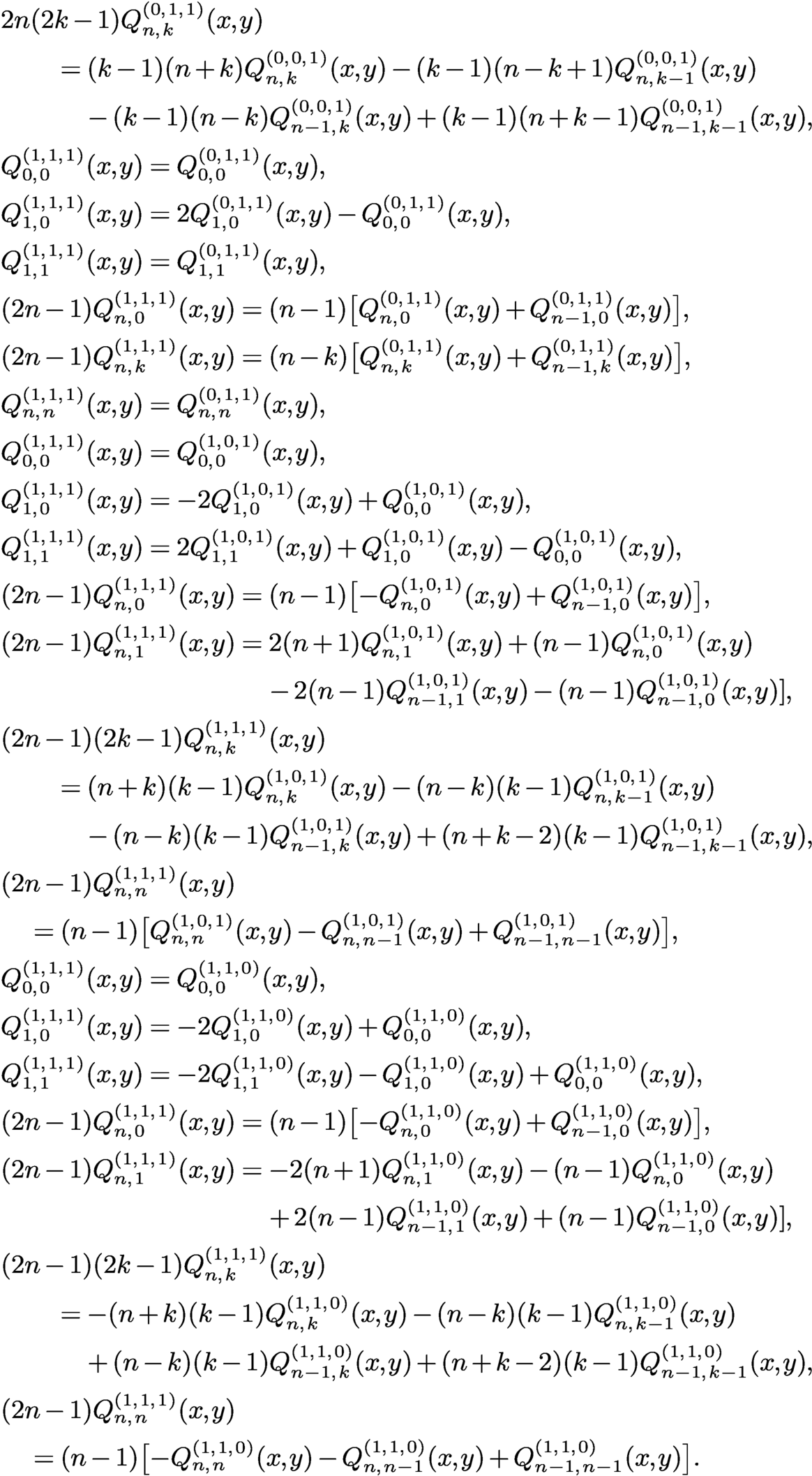 $$ \begin{align*} & Q_{0,0}^{(1,0,0)}(x,y) = P_{0,0}(x,y), \\ & (2n+1)Q_{n,k}^{(1,0,0)}(x,y) = (n-k)[P_{n,k}(x,y) + P_{n-1,k}(x,y) ],\\ & Q_{n,n}^{(1,0,0)}(x,y) = P_{n,n}(x,y), \\ & (2n+1)Q_{n,0}^{(0,1,0)}(x,y) = (n+1)P_{n,0}(x,y)-nP_{n-1,0}(x,y), \\ &\begin{aligned} (2n+1)Q_{n,k}^{(0,1,0)}(x,y) & = (n+k+1) P_{n,k}(x,y) -(n-k+1) P_{n,k-1}(x,y)\\ & \quad\, -(n-k)P_{n-1,k}(x,y)+(n+k) P_{n-1,k-1}(x,y), \end{aligned}\\ & (2n+1)Q_{n,0}^{(0,0,1)}(x,y) = (n+1)P_{n,0}(x,y)-nP_{n-1,0}(x,y), \\ &\begin{aligned} (2n+1)Q_{n,k}^{(0,0,1)}(x,y) & = -(n+k+1) P_{n,k}(x,y)-(n-k+1) P_{n,k-1}(x,y) \\ & \quad\, +(n-k)P_{n-1,k}(x,y)+(n+k) P_{n-1,k-1}(x,y), \end{aligned}\\ & Q_{0,0}^{(1,1,0)}(x,y) = Q_{0,0}^{(1,0,0)}(x,y), \\ & 2n Q_{n,0}^{(1,1,0)}(x,y) = (n+1)Q_{n,0}^{(1,0,0)}(x,y)- n Q_{n-1,0}^{(1,0,0)}(x,y), \\ &\begin{aligned} 4n Q_{n,k}^{(1,1,0)}(x,y) & = (n+k+1)Q_{n,k}^{(1,0,0)}(x,y)-(n-k)Q_{n,k-1}^{(1,0,0)}(x,y)\\ & \quad\, +(k-n)Q_{n-1,k}^{(1,0,0)}(x,y)+(n+k-1)Q_{n-1,k-1}^{(1,0,0)}(x,y), \end{aligned}\\ & 2Q_{n,n}^{(1,1,0)}(x,y) = Q_{n,n}^{(1,0,0)}(x,y)-Q_{n,n-1}^{(1,0,0)}(x,y)+Q_{n-1,n-1}^{(1,0,0)}(x,y) {,} \\ & 2 Q_{n,0}^{(1,1,0)}(x,y) = Q_{n,0}^{(0,1,0)}(x,y)+ Q_{n-1,0}^{(0,1,0)}(x,y), \\ & 2n Q_{n,k}^{(1,1,0)}(x,y) = (n-k)\bigl[Q_{n,k}^{(0,1,0)}(x,y)+Q_{n-1,k}^{(0,1,0)}(x,y)\bigr],\\ & Q_{n,n}^{(1,1,0)}(x,y) = Q_{n,n}^{(0,1,0)}(x,y) {,} \\ & Q_{0,0}^{(1,0,1)}(x,y) = Q_{0,0}^{(1,0,0)}(x,y), \\ & 2n Q_{n,0}^{(1,0,1)}(x,y) = (n+1)Q_{n,0}^{(1,0,0)}(x,y)- n Q_{n-1,0}^{(1,0,0)}(x,y), \\ &\begin{aligned} 4n Q_{n,k}^{(1,0,1)}(x,y) & = -(n+k+1)Q_{n,k}^{(1,0,0)}(x,y)-(n-k)Q_{n,k-1}^{(1,0,0)}(x,y)\\ & \quad\, +(n-k)Q_{n-1,k}^{(1,0,0)}(x,y)+(n+k-1)Q_{n-1,k-1}^{(1,0,0)}(x,y), \end{aligned}\\ & 2Q_{n,n}^{(1,0,1)}(x,y) = -Q_{n,n}^{(1,0,0)}(x,y)-Q_{n,n-1}^{(1,0,0)}(x,y)+Q_{n-1,n-1}^{(1,0,0)}(x,y){,} \\ & 2 Q_{n,0}^{(1,0,1)}(x,y) = Q_{n,0}^{(0,0,1)}(x,y)+ Q_{n-1,0}^{(0,0,1)}(x,y), \\ & 2n Q_{n,k}^{(1,0,1)}(x,y) = (n-k)\bigl[Q_{n,k}^{(0,0,1)}(x,y)+Q_{n-1,k}^{(0,0,1)}(x,y)\bigr],\\ & 2 Q_{n,0}^{(0,1,1)}(x,y) = -Q_{n,0}^{(0,1,0)}(x,y)+ Q_{n-1,0}^{(0,1,0)}(x,y), \\ &\begin{aligned} 2n Q_{n,1}^{(0,1,1)}(x,y) & = -2(n+1)Q_{n,1}^{(0,1,0)}(x,y)-n Q_{n,0}^{(0,1,0)}(x,y)\\ &\quad\, + 2(n-1)Q_{n-1,1}^{(0,1,0)}(x,y) +n Q_{n-1,0}^{(0,1,0)}(x,y), \end{aligned}\\ &\begin{aligned} & 2n(2k-1) Q_{n,k}^{(0,1,1)}(x,y) \\ & \qquad = -(k-1)(n+k) Q_{n,k}^{(0,1,0)}(x,y)-(k-1)(n-k+1)Q_{n,k-1}^{(0,1,0)}(x,y)\\ & \qquad\quad\, +(k-1)(n-k) Q_{n-1,k}^{(0,1,0)}(x,y)+(k-1)(n+k-1)Q_{n-1,k-1}^{(0,1,0)}(x,y){,} \end{aligned}\\ & 2 Q_{n,0}^{(0,1,1)}(x,y) = -Q_{n,0}^{(0,0,1)}(x,y)+ Q_{n-1,0}^{(0,0,1)}(x,y), \\ &\begin{aligned} 2n Q_{n,1}^{(0,1,1)}(x,y) & = 2(n+1)Q_{n,1}^{(0,1,0)}(x,y)+n Q_{n,0}^{(0,0,1)}(x,y)\\ & \quad\, -2(n-1)Q_{n-1,1}^{(0,1,0)}(x,y) -n Q_{n-1,0}^{(0,0,1)}(x,y), \end{aligned}\\ &\begin{aligned} & 2n(2k-1) Q_{n,k}^{(0,1,1)}(x,y) \\ &\qquad = (k-1)(n+k)Q_{n,k}^{(0,0,1)}(x,y) -(k-1)(n-k+1)Q_{n,k-1}^{(0,0,1)}(x,y)\\ & \qquad\quad\, -(k-1)(n-k)Q_{n-1,k}^{(0,0,1)}(x,y) +(k-1)(n+k-1)Q_{n-1,k-1}^{(0,0,1)}(x,y) {,} \end{aligned}\\ & Q_{0,0}^{(1,1,1)}(x,y) = Q_{0,0}^{(0,1,1)}(x,y), \\ & Q_{1,0}^{(1,1,1)}(x,y) = 2Q_{1,0}^{(0,1,1)}(x,y) -Q_{0,0}^{(0,1,1)}(x,y), \\ & Q_{1,1}^{(1,1,1)}(x,y) = Q_{1,1}^{(0,1,1)}(x,y), \\ & (2n-1)Q_{n,0}^{(1,1,1)}(x,y) = (n-1)\bigl[Q_{n,0}^{(0,1,1)}(x,y) +Q_{n-1,0}^{(0,1,1)}(x,y)\bigr], \\ & (2n-1)Q_{n,k}^{(1,1,1)}(x,y) = (n-k)\bigl[Q_{n,k}^{(0,1,1)}(x,y) +Q_{n-1,k}^{(0,1,1)}(x,y)\bigr], \\ & Q_{n,n}^{(1,1,1)}(x,y) = Q_{n,n}^{(0,1,1)}(x,y){,} \\ & Q_{0,0}^{(1,1,1)}(x,y) = Q_{0,0}^{(1,0,1)}(x,y), \\ & Q_{1,0}^{(1,1,1)}(x,y) = -2Q_{1,0}^{(1,0,1)}(x,y) +Q_{0,0}^{(1,0,1)}(x,y), \\ & Q_{1,1}^{(1,1,1)}(x,y) = 2Q_{1,1}^{(1,0,1)}(x,y)+Q_{1,0}^{(1,0,1)}(x,y)-Q_{0,0}^{(1,0,1)}(x,y), \\ & (2n-1)Q_{n,0}^{(1,1,1)}(x,y) = (n-1)\bigl[-Q_{n,0}^{(1,0,1)}(x,y) +Q_{n-1,0}^{(1,0,1)}(x,y)\bigr], \\ &\begin{aligned} (2n-1)Q_{n,1}^{(1,1,1)}(x,y) & = 2 (n+1)Q_{n,1}^{(1,0,1)}(x,y) +(n-1) Q_{n,0}^{(1,0,1)}(x,y) \\ & \quad\, -2(n-1) Q_{n-1,1}^{(1,0,1)}(x,y) -(n-1)Q_{n-1,0}^{(1,0,1)}(x,y)], \end{aligned}\\ &\begin{aligned} & (2n-1)(2k-1)Q_{n,k}^{(1,1,1)}(x,y) \\ & \qquad= (n+k)(k-1) Q_{n,k}^{(1,0,1)}(x,y) -(n-k)(k-1)Q_{n,k-1}^{(1,0,1)}(x,y)\\ & \qquad\quad\, -(n-k)(k-1) Q_{n-1,k}^{(1,0,1)}(x,y) +(n+k-2)(k-1)Q_{n-1,k-1}^{(1,0,1)}(x,y), \end{aligned}\\ &\begin{aligned} & (2n-1)Q_{n,n}^{(1,1,1)}(x,y) \\ & \quad = (n-1) \bigl[Q_{n,n}^{(1,0,1)}(x,y)-Q_{n,n-1}^{(1,0,1)}(x,y)+Q_{n-1,n-1}^{(1,0,1)}(x,y)\bigr]{,} \end{aligned}\\ & Q_{0,0}^{(1,1,1)}(x,y) = Q_{0,0}^{(1,1,0)}(x,y), \\ & Q_{1,0}^{(1,1,1)}(x,y) = -2Q_{1,0}^{(1,1,0)}(x,y) +Q_{0,0}^{(1,1,0)}(x,y), \\ & Q_{1,1}^{(1,1,1)}(x,y) = -2Q_{1,1}^{(1,1,0)}(x,y)-Q_{1,0}^{(1,1,0)}(x,y)+Q_{0,0}^{(1,1,0)}(x,y), \\ & (2n-1)Q_{n,0}^{(1,1,1)}(x,y) = (n-1)\bigl[-Q_{n,0}^{(1,1,0)}(x,y) +Q_{n-1,0}^{(1,1,0)}(x,y)\bigr], \\ &\begin{aligned} (2n-1)Q_{n,1}^{(1,1,1)}(x,y) & = -2 (n+1)Q_{n,1}^{(1,1,0)}(x,y) -(n-1) Q_{n,0}^{(1,1,0)}(x,y) \\ & \quad\, +2(n-1) Q_{n-1,1}^{(1,1,0)}(x,y) +(n-1)Q_{n-1,0}^{(1,1,0)}(x,y)], \end{aligned}\\ &\begin{aligned} &(2n-1)(2k-1)Q_{n,k}^{(1,1,1)}(x,y) \\ & \qquad = -(n+k)(k-1) Q_{n,k}^{(1,1,0)}(x,y) -(n-k)(k-1)Q_{n,k-1}^{(1,1,0)}(x,y) \\ & \qquad\quad\, +(n-k)(k-1) Q_{n-1,k}^{(1,1,0)}(x,y) +(n+k-2)(k-1)Q_{n-1,k-1}^{(1,1,0)}(x,y), \end{aligned}\\ &\begin{aligned} &(2n-1)Q_{n,n}^{(1,1,1)}(x,y) \\ & \quad = (n-1) \bigl[-Q_{n,n}^{(1,1,0)}(x,y)-Q_{n,n-1}^{(1,1,0)}(x,y)+Q_{n-1,n-1}^{(1,1,0)}(x,y)\bigr]. \end{aligned} \end{align*} $$
These define the conversion operators
 $$ \begin{align*} \boldsymbol{Q}^{(a,b,c)} = \boldsymbol{P}^{(0,0,0)} \tilde R_{(a,b,c)}^{(0,0,0)}. \end{align*} $$
Proposition B.8 (derivatives (Olver et al. Reference Olver, Townsend and Vasil2019, Corollary C.4)).
The following recurrence relationships hold:
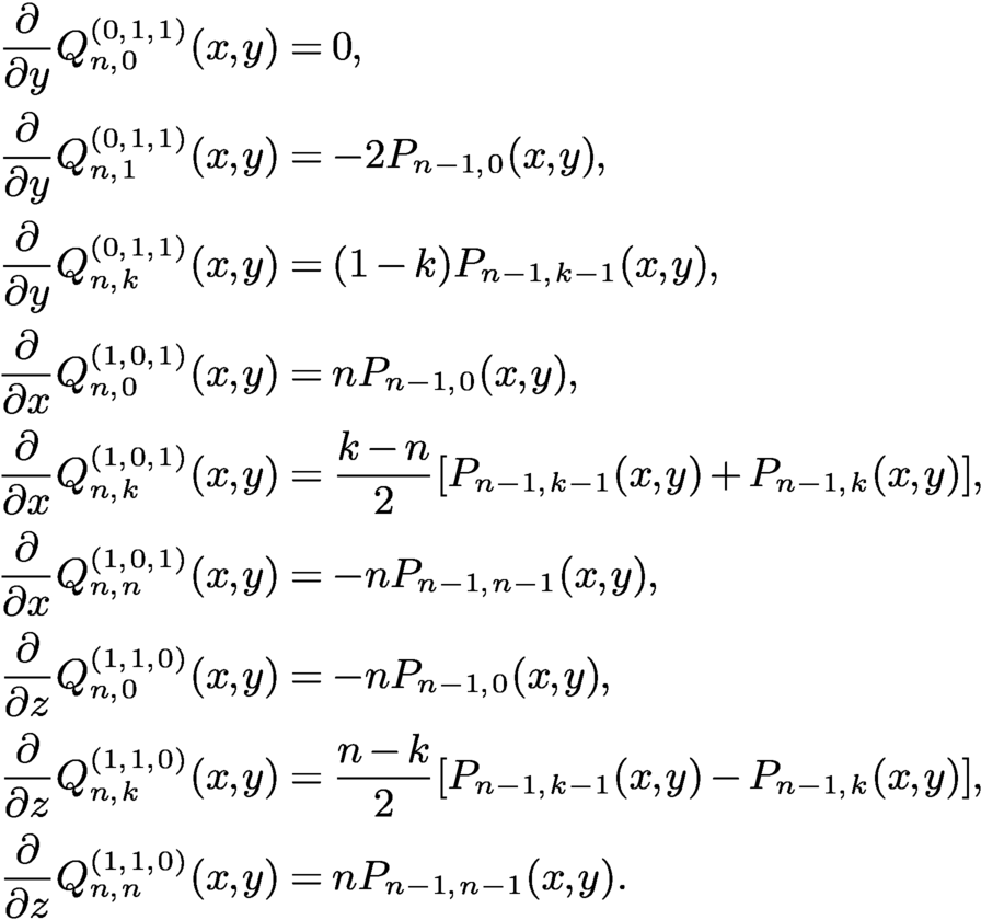 $$ \begin{align*} \displaystyle \frac{\partial }{ \partial y} Q_{n,0}^{(0,1,1)}(x,y) & = 0, \\ \displaystyle \frac{\partial }{ \partial y} Q_{n,1}^{(0,1,1)}(x,y) & = -2 P_{n-1,0}(x,y), \\ \displaystyle \frac{\partial }{ \partial y} Q_{n,k}^{(0,1,1)}(x,y) & = (1-k) P_{n-1,k-1}(x,y), \\ \displaystyle \frac{\partial }{ \partial x} Q_{n,0}^{(1,0,1)}(x,y) & = n P_{n-1,0}(x,y), \\ \displaystyle \frac{\partial }{ \partial x} Q_{n,k}^{(1,0,1)}(x,y) & = \displaystyle \frac{k-n }{ 2} [{P_{n-1,k-1}(x,y) +P_{n-1,k}(x,y)}],\\ \displaystyle \frac{\partial }{ \partial x} Q_{n,n}^{(1,0,1)}(x,y) & = -n P_{n-1,n-1}(x,y), \\ \displaystyle \frac{\partial }{ \partial z} Q_{n,0}^{(1,1,0)}(x,y) & = -n P_{n-1,0}(x,y), \\ \displaystyle \frac{\partial }{ \partial z} Q_{n,k}^{(1,1,0)}(x,y) & = \displaystyle \frac{n-k }{ 2} [{P_{n-1,k-1}(x,y) - P_{n-1,k}(x,y)}],\\ \displaystyle \frac{\partial }{ \partial z} Q_{n,n}^{(1,1,0)}(x,y) & = n P_{n-1,n-1}(x,y). \end{align*} $$
These define the derivative operators
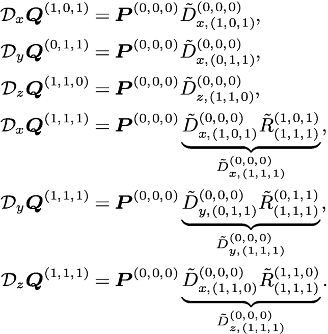 $$ \begin{align*} {\mathcal D}_x \boldsymbol{Q}^{(1,0,1)} & = \boldsymbol{P}^{(0,0,0)} \tilde D_{x,(1,0,1)}^{(0,0,0)}, \\ {\mathcal D}_y \boldsymbol{Q}^{(0,1,1)} & = \boldsymbol{P}^{(0,0,0)} \tilde D_{x,(0,1,1)}^{(0,0,0)}, \\ {\mathcal D}_z \boldsymbol{Q}^{(1,1,0)} & = \boldsymbol{P}^{(0,0,0)} \tilde D_{z,(1,1,0)}^{(0,0,0)}, \\ {\mathcal D}_x \boldsymbol{Q}^{(1,1,1)} & = \boldsymbol{P}^{(0,0,0)} \underbrace{\tilde D_{x,(1,0,1)}^{(0,0,0)} \tilde R_{(1,1,1)}^{(1,0,1)}}_{\tilde D_{x,(1,1,1)}^{(0,0,0)}}, \\ {\mathcal D}_y \boldsymbol{Q}^{(1,1,1)} & = \boldsymbol{P}^{(0,0,0)} \underbrace{\tilde D_{y,(0,1,1)}^{(0,0,0)} \tilde R_{(1,1,1)}^{(0,1,1)}}_{\tilde D_{y,(1,1,1)}^{(0,0,0)}}, \\ {\mathcal D}_z \boldsymbol{Q}^{(1,1,1)} & = \boldsymbol{P}^{(0,0,0)} \underbrace{\tilde D_{x,(1,1,0)}^{(0,0,0)} \tilde R_{(1,1,1)}^{(1,1,0)}}_{\tilde D_{z,(1,1,1)}^{(0,0,0)}}. \end{align*} $$
Proposition B.9 (restriction (Olver et al. Reference Olver, Townsend and Vasil2019, Proposition B.2)).
The restriction operator to
 $x = 0$
is given by
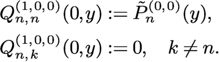 $$ \begin{align*} Q_{n,n}^{(1,0,0)}(0,y) &:= \tilde P_{n}^{(0,0)}(y), \\ Q_{n,k}^{(1,0,0)}(0,y) &:= 0, \quad k \neq n. \end{align*} $$
The restriction operator to
 $y = 0$
is given by
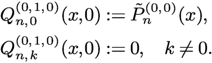 $$ \begin{align*} Q_{n,0}^{(0,1,0)}(x,0) &:= \tilde P_{n}^{(0,0)}(x), \\ Q_{n,k}^{(0,1,0)}(x,0) &:= 0, \quad k \neq 0. \end{align*} $$
The restriction operator to
 $z = 0$
is given by
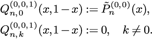 $$ \begin{align*} Q_{n,0}^{(0,0,1)}(x,1-x) &:= \tilde P_{n}^{(0,0)}(x), \\ Q_{n,k}^{(0,0,1)}(x,1-x) &:= 0, \quad k \neq 0. \end{align*} $$
We denote these as
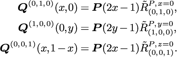 $$ \begin{align*} \boldsymbol{Q}^{(0,1,0)}(x,0) &= \boldsymbol{P}(2x-1)\tilde R_{(0,1,0)}^{P,x=0}, \\ \boldsymbol{Q}^{(1,0,0)}(0,y) &= \boldsymbol{P}(2y-1) \tilde R_{(1,0,0)}^{P,y=0}, \\ \boldsymbol{Q}^{(0,0,1)}(x,1-x) &= \boldsymbol{P}(2x-1) \tilde R_{(0,0,1)}^{P,z=0}. \end{align*} $$
These then give
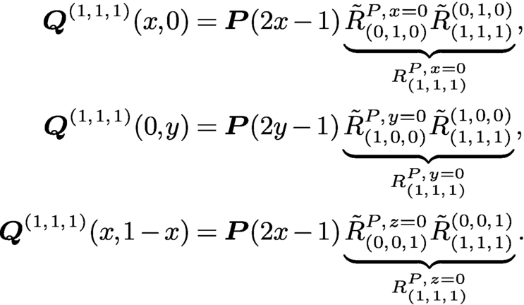 $$ \begin{align*} \boldsymbol{Q}^{(1,1,1)}(x,0) &= \boldsymbol{P}(2x-1) \underbrace{ \tilde R_{(0,1,0)}^{P,x=0} \tilde R_{(1,1,1)}^{(0,1,0)}}_{R_{(1,1,1)}^{P,x=0}}, \\ \boldsymbol{Q}^{(1,1,1)}(0,y) &= \boldsymbol{P}(2y-1) \underbrace{ \tilde R_{(1,0,0)}^{P,y=0} \tilde R_{(1,1,1)}^{(1,0,0)}}_{R_{(1,1,1)}^{P,y=0}}, \\ \boldsymbol{Q}^{(1,1,1)}(x,1-x) &= \boldsymbol{P}(2x-1) \underbrace{ \tilde R_{(0,0,1)}^{P,z=0} \tilde R_{(1,1,1)}^{(0,0,1)}}_{R_{(1,1,1)}^{P,z=0}}. \end{align*} $$
C Semiclassical orthogonal polynomials
Given a family of classical orthogonal polynomials
 $$ \begin{align*} p_{n+1}(x) = (A_nx+B_n)p_n(x) - C_np_{n-1}(x),\quad p_0(x) = 1, \end{align*} $$
the associated orthogonal polynomials are those polynomials with the same initial conditions that use the classical recurrence coefficients with indices offset by
 $c\in \mathbb {N}$
units:
 $$ \begin{align*} p_{n+1}(x;c) = (A_{n+c}x+B_{n+c})p_n(x;c) - C_{n+c}p_{n-1}(x;c). \end{align*} $$
They too satisfy a linear homogeneous differential equation (Zarzo, Ronveaux and Godoy Reference Zarzo, Ronveaux and Godoy1993):
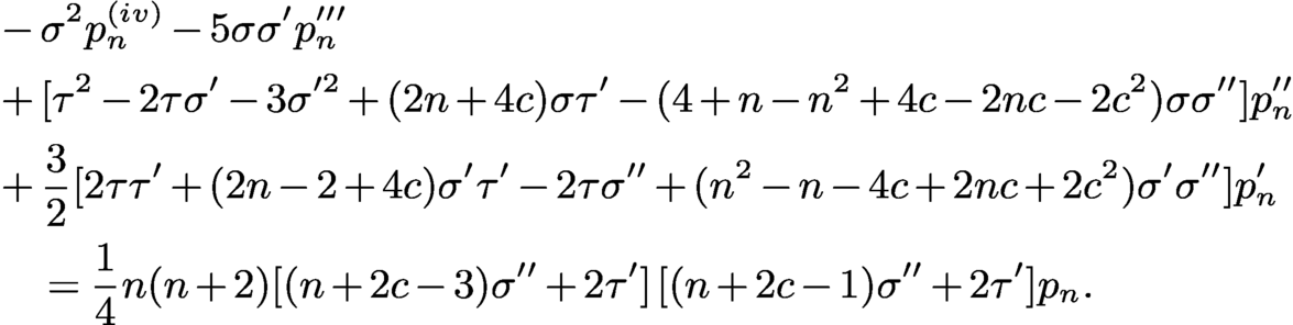 $$ \begin{align*} & -\sigma^2 p_n^{\mathrm (iv)} - 5\sigma \sigma' p_n^{\prime\prime\prime}\\ & + [\tau^2-2\tau\sigma'-3\sigma^{\prime{2}}+(2n+4c)\sigma\tau'-(4+n-n^2+4c-2nc-2c^2)\sigma\sigma^{\prime\prime}] p_n^{\prime\prime}\nonumber\\ & + \displaystyle \frac{3}{2}[2\tau\tau' + (2n-2+4c)\sigma'\tau'-2\tau\sigma^{\prime\prime} + (n^2-n-4c+2nc+2c^2)\sigma'\sigma^{\prime\prime}] p_n'\nonumber\\ & \quad = \displaystyle \frac{1}{4} n(n+2)[(n+2c-3)\sigma^{\prime\prime}+2\tau']\, [(n+2c-1)\sigma^{\prime\prime}+2\tau']p_n\nonumber. \end{align*} $$
Associated orthogonal polynomials have applications through their diagonalization of the following Stieltjes transforms (Erdélyi et al. Reference Erdélyi1953, vol. 2, p. 162 (6)):
 $$ \begin{align*} p_n(x;c+1) = \dfrac{1}{A_c\int_D \mathrm{d}\mu(t;c)}\int_D\dfrac{p_{n+1}(x;c)-p_{n+1}(t;c)}{x-t}{\mathrm\,d}\mu(t;c). \end{align*} $$
(Generalized) co-recursive orthogonal polynomials are related to the associated orthogonal polynomials. They too satisfy fourth-order linear homogeneous differential equations, though we refer the interested reader to Ronveaux and Marcellán (Reference Ronveaux and Marcellán1989) and in particular to Ronveaux, Zarzo and Godoy (Reference Ronveaux, Zarzo and Godoy1995) for their coefficients.
Konoplev orthogonal polynomials (Konoplev Reference Konoplev1961) are another semiclassical case that are orthogonal with respect to
 $L^2([-1,1],|x|^\gamma (1-x^2)^\alpha {\mathrm \,d}x)$
. They are the polynomial eigenfunctions of
 $$ \begin{align*} \{(1-x^2)^{-\alpha}|x|^{2-\gamma}(-{\mathcal D})[|x|^\gamma(1-x^2)^{\alpha+1}{\mathcal D}] + \delta_n\gamma\} u = n(n+2\alpha+\gamma+1)x^2 u, \end{align*} $$
where
 $\delta _n = (1-(-1)^n)/2$
. Note that there is a sign error in Konoplev (Reference Konoplev1961). Konoplev orthogonal polynomials are an example where the weight is a product of algebraic factors. Other examples arise when the domain is a subset of
 $[-1,1]$
. It is also possible to develop a linear differential equation with polynomial coefficiesnts for these orthogonal polynomials (Magnus Reference Magnus1995).
Bochner (Reference Bochner1929) and Krall (Reference Krall1938) characterized orthogonal polynomial systems that are solutions of linear differential eigenvalue problems with polynomial coefficients independent of the degree. Their generalized polynomials are all orthogonal with respect to measures of classical orthogonal polynomials with added Dirac distributions at the endpoints. They may satisfy fourth, sixth or infinite-order linear differential eigenvalue problems.
D Notation
D.1 Continuous operators
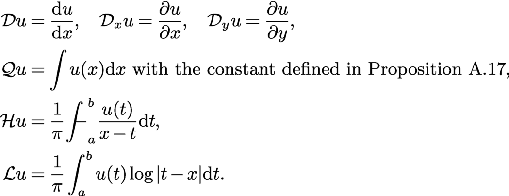 $$ \begin{align*} {\mathcal D} u & = \displaystyle \frac{{\mathrm{d}} u }{ {{\mathrm{d}}x}} ,\quad {\mathcal D}_x u = \displaystyle \frac{\partial u }{ \partial x}, \quad {\mathcal D}_y u = \displaystyle \frac{\partial u }{ \partial y}, \\ {\mathcal Q} u & = \int u(x) {{\mathrm{d}}x} \text{ with the constant defined in Proposition~A.17} ,\\ {\mathcal H} u & = \displaystyle \frac{1 }{ \pi} {\int\!\!\!\!\!\!-}_a^b \displaystyle \frac{u(t) }{ x - t} {{\mathrm{d}}t}, \\ {\mathcal L} u & = \displaystyle \frac{1 }{ \pi} \int_a^b u(t) \log|t-x| {{\mathrm{d}}t}. \end{align*} $$
D.2 Univariate
Quasimatrix notation:
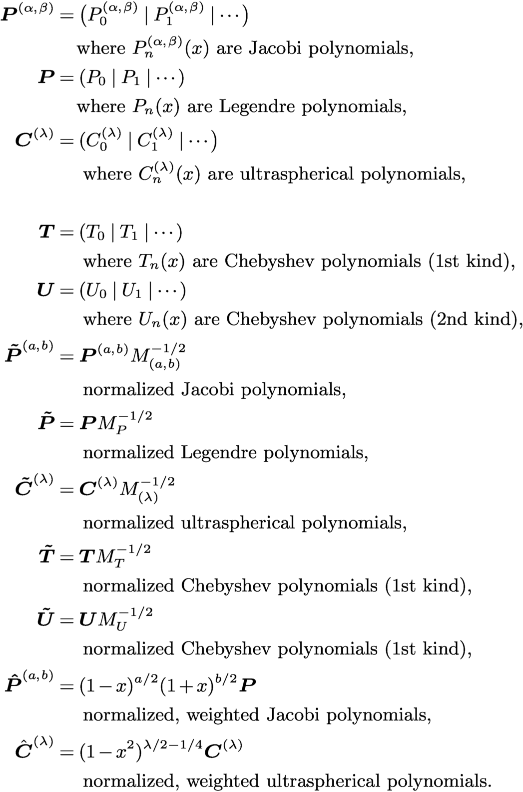 $$ \begin{align*} \boldsymbol{P}^{(\alpha,\beta)} & = \big(P_{0}^{(\alpha,\beta)} \mid P_{1}^{(\alpha,\beta)} \mid \cdots\big) \\ &\quad\, \text{where } P_n^{(\alpha,\beta)}(x) \text{ are Jacobi polynomials,} \\ \boldsymbol{P} &= (P_0 \mid P_1\mid \cdots) \\ &\quad\, \text{where } P_n(x) \text{ are Legendre polynomials,} \\ \boldsymbol{C}^{(\lambda)} &= (C_{0}^{(\lambda)} \mid C_{1}^{(\lambda)} \mid \cdots\big) \\ &\quad~\, \text{where } C_n^{(\lambda)}(x) \text{ are ultraspherical polynomials,} \\ \\ \boldsymbol{T} &= (T_0 \mid T_1 \mid \cdots) \\ &\quad~\, \text{where } T_n(x) \text{ are Chebyshev polynomials (1st kind),} \\ \boldsymbol{U} &= (U_0 \mid U_1 \mid \cdots) \\ &\quad~\, \text{where } U_n(x) \text{ are Chebyshev polynomials (2nd kind),} \\ \boldsymbol{\tilde P}^{(a,b)} &= \boldsymbol{P}^{(a,b)} M_{(a,b)}^{-1/2} \\ &\quad~\, \text{normalized Jacobi polynomials,} \\ \boldsymbol{\tilde P} &= \boldsymbol{P} M_P^{-1/2} \\ &\quad~\, \text{normalized Legendre polynomials,} \\ \boldsymbol{\tilde C}^{(\lambda)} &= \boldsymbol{C}^{(\lambda)} M_{(\lambda)}^{-1/2} \\ &\quad~\, \text{normalized ultraspherical polynomials,} \\ \boldsymbol{\tilde T} &= \boldsymbol{T} M_T^{-1/2} \\ &\quad~\, \text{normalized Chebyshev polynomials (1st kind),} \\ \boldsymbol{\tilde U} &= \boldsymbol{U} M_U^{-1/2} \\ &\quad~\, \text{normalized Chebyshev polynomials (1st kind),} \\ \boldsymbol{\hat P}^{(a,b)} &= (1-x)^{a/2} (1+x)^{b/2} \boldsymbol{P} \\ &\quad~\, \text{normalized, weighted Jacobi polynomials,} \\ \hat{\boldsymbol{C}}^{(\lambda)} &= (1-x^2)^{\lambda/2-1/4} \boldsymbol{C}^{(\lambda)} \\ &\quad~\, \text{normalized, weighted ultraspherical polynomials.} \end{align*} $$
Multiplication operators:
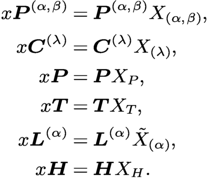 $$ \begin{align*} x \boldsymbol{P}^{(\alpha,\beta)} & = \boldsymbol{P}^{(\alpha,\beta)} X_{(\alpha,\beta)}, \\ x \boldsymbol{C}^{(\lambda)} & = \boldsymbol{C}^{(\lambda)} X_{(\lambda)}, \\ x \boldsymbol{P} & = \boldsymbol{P} X_P {,} \\ x \boldsymbol{T} & = \boldsymbol{T} X_T, \\ x \boldsymbol{L}^{(\alpha)} & = \boldsymbol{L}^{(\alpha)} \tilde X_{(\alpha)}, \\ x \boldsymbol{H} & = \boldsymbol{H} X_H. \end{align*} $$
Conversion operators:
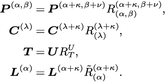 $$ \begin{align*} \boldsymbol{P}^{(\alpha,\beta)} & = \boldsymbol{P}^{(\alpha+\kappa,\beta+\nu)} R_{(\alpha,\beta)}^{(\alpha+\kappa,\beta+\nu)}, \\ \boldsymbol{C}^{(\lambda)} & = \boldsymbol{C}^{(\lambda+\kappa)} R_{(\lambda)}^{(\lambda+\kappa)}, \\ \boldsymbol{T} & = \boldsymbol{U} R_T^U, \\ \boldsymbol{L}^{(\alpha)} & = \boldsymbol{L}^{(\alpha+\kappa)} \tilde R_{(\alpha)}^{(\alpha+\kappa)}. \end{align*} $$
Weighted conversion operators:
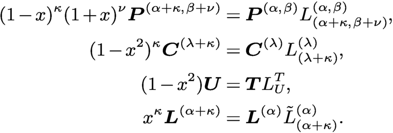 $$ \begin{align*} (1-x)^\kappa (1+x)^\nu \boldsymbol{P}^{(\alpha+\kappa,\beta+\nu)} & = \boldsymbol{P}^{(\alpha,\beta)} L_{(\alpha+\kappa,\beta+\nu)}^{(\alpha,\beta)}, \\ (1-x^2)^\kappa \boldsymbol{C}^{(\lambda+\kappa)} & = \boldsymbol{C}^{(\lambda)} L_{(\lambda+\kappa)}^{(\lambda)}, \\ (1-x^2) \boldsymbol{U} & = \boldsymbol{T} L_U^T, \\ x^\kappa \boldsymbol{L}^{(\alpha+\kappa)} & = \boldsymbol{L}^{(\alpha)} \tilde L_{(\alpha+\kappa)}^{(\alpha)}. \end{align*} $$
Differentiation operators:
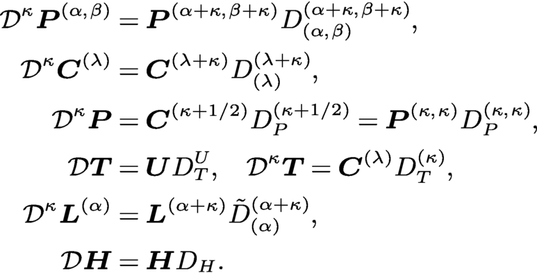 $$ \begin{align*} {\mathcal D}^\kappa \boldsymbol{P}^{(\alpha,\beta)} & = \boldsymbol{P}^{(\alpha+\kappa,\beta+\kappa)} D_{(\alpha,\beta)}^{(\alpha+\kappa,\beta+\kappa)}, \\ {\mathcal D}^\kappa \boldsymbol{C}^{(\lambda)} & = \boldsymbol{C}^{(\lambda+\kappa)} D_{(\lambda)}^{(\lambda+\kappa)}, \\ {\mathcal D}^\kappa \boldsymbol{P} & = \boldsymbol{C}^{(\kappa+1/2)} D_P^{(\kappa+1/2)} = \boldsymbol{P}^{(\kappa,\kappa)} D_P^{(\kappa,\kappa)} {,} \\ {\mathcal D} \boldsymbol{T} & = \boldsymbol{U} D_T^U, \quad {\mathcal D}^\kappa \boldsymbol{T} = \boldsymbol{C}^{(\lambda)} D_T^{(\kappa)} {,} \\ {\mathcal D}^\kappa \boldsymbol{L}^{(\alpha)} & = \boldsymbol{L}^{(\alpha+\kappa)} \tilde D_{(\alpha)}^{(\alpha+\kappa)}, \\ {\mathcal D} \boldsymbol{H} & = \boldsymbol{H} D_H. \end{align*} $$
Weighted differentiation operators:
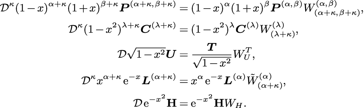 $$ \begin{align*} {\mathcal D}^\kappa (1-x)^{\alpha+\kappa} (1+x)^{\beta+\kappa} \boldsymbol{P}^{(\alpha+\kappa,\beta+\kappa)} & = (1-x)^{\alpha} (1+x)^{\beta} \boldsymbol{P}^{(\alpha,\beta)} W_{(\alpha+\kappa,\beta+\kappa)}^{(\alpha,\beta)},\\ {\mathcal D}^\kappa (1-x^2)^{\lambda+\kappa} \boldsymbol{C}^{(\lambda+\kappa)} & = (1-x^2)^{\lambda} \boldsymbol{C}^{(\lambda)} W_{(\lambda+\kappa)}^{(\lambda)},\\ {\mathcal D} \sqrt{1-x^2} \boldsymbol{U} & = \displaystyle \frac{\boldsymbol{T} }{ \sqrt{1-x^2}} W_U^T, \\ {\mathcal D}^\kappa x^{\alpha+\kappa} \,{\mathrm{e}}^{-x} \boldsymbol{L}^{(\alpha+\kappa)} & = x^\alpha \,{\mathrm{e}}^{-x} \boldsymbol{L}^{(\alpha)} \tilde W_{(\alpha+\kappa)}^{(\alpha)},\\ {\mathcal D} \,{\mathrm{e}}^{-x^2} \mathbf H & = {\mathrm{e}}^{-x^2} \mathbf H W_H. \end{align*} $$
One-sided weighted differentiation operators:
 $$ \begin{align*} {\mathcal D}^\kappa (1-x)^{\alpha+\kappa} \boldsymbol{P}^{(\alpha+\kappa,\beta)} & = (1-x)^{\alpha} \boldsymbol{P}^{(\alpha,\beta+\kappa)} W_{{\mathrm L},(\alpha,\beta)}^{(\alpha,\beta+\kappa)}, \\ {\mathcal D} (1+x)^{\beta+\kappa} \boldsymbol{P}^{(\alpha,\beta+\kappa)} & = (1+x)^\beta \boldsymbol{P}^{(\alpha+\kappa,\beta)} W_{{\mathrm R},(\alpha,\beta)}^{(\alpha+\kappa,\beta)}. \end{align*} $$
Singular integral operators:
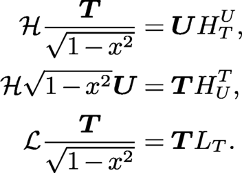 $$ \begin{align*} {\mathcal H} \displaystyle \frac{\boldsymbol{T} }{ \sqrt{1-x^2}} & = \boldsymbol{U} H_T^U, \\ {\mathcal H} \sqrt{1-x^2} \boldsymbol{U} & = \boldsymbol{T} H_U^T, \\ {\mathcal L} \displaystyle \frac{\boldsymbol{T} }{ \sqrt{1-x^2}} & = \boldsymbol{T} L_T. \end{align*} $$
D.3 Bivariate orthogonal polynomials
Quasimatrix notation:
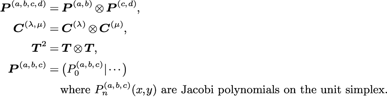 $$ \begin{align*} \boldsymbol{P}^{(a,b,c,d)} & = \boldsymbol{P}^{(a,b)} \otimes \boldsymbol{P}^{(c,d)}, \\ \boldsymbol{C}^{(\lambda,\mu)} & = \boldsymbol{C}^{(\lambda)} \otimes \boldsymbol{C}^{(\mu)}, \\ \boldsymbol{T}^{2} & = \boldsymbol{T} \otimes \boldsymbol{T}, \\ \boldsymbol{P}^{(a,b,c)} & = \big(P_0^{(a,b,c)}|\cdots \big) \\ &\quad~\,\!\!\! \text{where } P_n^{(a,b,c)}(x,y) \text{ are Jacobi polynomials on the unit simplex.} \end{align*} $$
Multiplication operators:
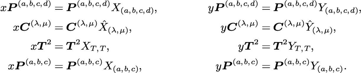 $$ \begin{align*} x \boldsymbol{P}^{(a,b,c,d)} & = \boldsymbol{P}^{(a,b,c,d)} X_{(a,b,c,d)}, & \quad y \boldsymbol{P}^{(a,b,c,d)} &= \boldsymbol{P}^{(a,b,c,d)} Y_{(a,b,c,d)}, \\ x \boldsymbol{C}^{(\lambda,\mu)} & = \boldsymbol{C}^{(\lambda,\mu)} \hat X_{(\lambda,\mu)}, & y \boldsymbol{C}^{(\lambda,\mu)} &= \boldsymbol{C}^{(\lambda,\mu)} \hat Y_{(\lambda,\mu)}, \\ x \boldsymbol{T}^2 & = \boldsymbol{T}^2 X_{T,T}, & y \boldsymbol{T}^2 &= \boldsymbol{T}^2 Y_{T,T}, \\ x \boldsymbol{P}^{(a,b,c)} & = \boldsymbol{P}^{(a,b,c)} X_{(a,b,c)}, & y \boldsymbol{P}^{(a,b,c)} &= \boldsymbol{P}^{(a,b,c)} Y_{(a,b,c)}. \end{align*} $$
Conversion operators:
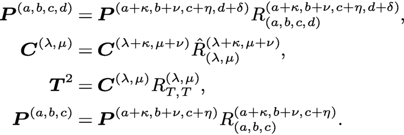 $$ \begin{align*} \boldsymbol{P}^{(a,b,c,d)}& = \boldsymbol{P}^{(a+\kappa,b+\nu,c+\eta,d+\delta)} R_{(a,b,c,d)}^{(a+\kappa,b+\nu,c+\eta,d+\delta)}, \\ \boldsymbol{C}^{(\lambda,\mu)}& = \boldsymbol{C}^{(\lambda+\kappa,\mu+\nu)} \hat R_{(\lambda,\mu)}^{(\lambda+\kappa,\mu+\nu)}, \\ \boldsymbol{T}^2 & = \boldsymbol{C}^{(\lambda,\mu)} R_{T,T}^{(\lambda,\mu)}, \\ \boldsymbol{P}^{(a,b,c)} & = \boldsymbol{P}^{(a+\kappa,b+\nu,c+\eta)} R_{(a,b,c)}^{(a+\kappa,b+\nu,c+\eta)}. \end{align*} $$
Weighted conversion operators (
 $z = 1-x-y$
):
 $$ \begin{align*} x^\kappa y^\nu z^\eta \boldsymbol{P}^{(a+\kappa,b+\nu,c+\eta)} = \boldsymbol{P}^{(a,b,c)} L_{(a+\kappa,b+\nu,c+\eta)}^{(a,b,c)} {.} \end{align*} $$
Differentiation operators (
 ${\mathcal D}_z = {\mathcal D}_y - {\mathcal D}_x$
,
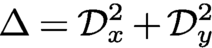 $\Delta = {\mathcal D}_x^2 + {\mathcal D}_y^2$
):
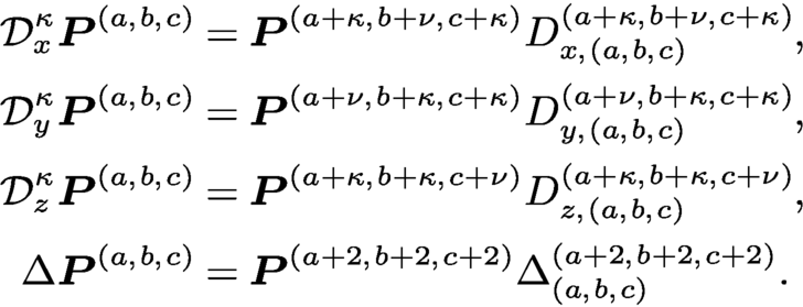 $$ \begin{align*} {\mathcal D}_x^\kappa\boldsymbol{P}^{(a,b,c)} & = \boldsymbol{P}^{(a+\kappa,b+\nu,c+\kappa)} D_{x,(a,b,c)}^{(a+\kappa,b+\nu,c+\kappa)}, \\ {\mathcal D}_y^\kappa\boldsymbol{P}^{(a,b,c)} & = \boldsymbol{P}^{(a+\nu,b+\kappa,c+\kappa)} D_{y,(a,b,c)}^{(a+\nu,b+\kappa,c+\kappa)}, \\ {\mathcal D}_z^\kappa\boldsymbol{P}^{(a,b,c)} & = \boldsymbol{P}^{(a+\kappa,b+\kappa,c+\nu)} D_{z,(a,b,c)}^{(a+\kappa,b+\kappa,c+\nu)}, \\ \Delta \boldsymbol{P}^{(a,b,c)} & = \boldsymbol{P}^{(a+2,b+2,c+2)} \Delta_{(a,b,c)}^{(a+2,b+2,c+2)}. \end{align*} $$
Weighted differentiation operators (
 $z = 1-x-y$
,
 ${\mathcal D}_z = {\mathcal D}_y - {\mathcal D}_x$
,
 $\Delta = {\mathcal D}_x^2 + {\mathcal D}_y^2$
):
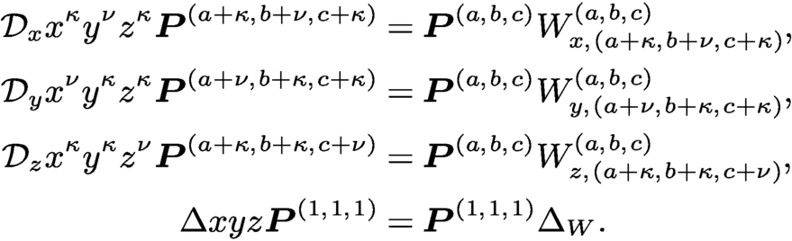 $$ \begin{align*} {\mathcal D}_x x^\kappa y^\nu z^\kappa \boldsymbol{P}^{(a+\kappa,b+\nu,c+\kappa)} & = \boldsymbol{P}^{(a,b,c)} W_{x,(a+\kappa,b+\nu,c+\kappa)}^{(a,b,c)}, \\ {\mathcal D}_y x^\nu y^\kappa z^\kappa \boldsymbol{P}^{(a+\nu,b+\kappa,c+\kappa)} & = \boldsymbol{P}^{(a,b,c)} W_{y,(a+\nu,b+\kappa,c+\kappa)}^{(a,b,c)}, \\ {\mathcal D}_z x^\kappa y^\kappa z^\nu \boldsymbol{P}^{(a+\kappa,b+\kappa,c+\nu)} & = \boldsymbol{P}^{(a,b,c)} W_{z,(a+\kappa,b+\kappa,c+\nu)}^{(a,b,c)}, \\ \Delta x y z \boldsymbol{P}^{(1,1,1)} & = \boldsymbol{P}^{(1,1,1)} \Delta_W. \end{align*} $$