


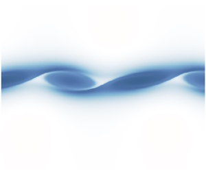





1. Introduction
Kelvin–Helmholtz instability (KHI) is believed to be important in geophysical flows found in both the oceans (Smyth & Moum Reference Smyth and Moum2012) and atmosphere (Fukao et al. Reference Fukao, Luce, Mega and Yamamoto2011; Sun et al. Reference Sun2015). Of particular importance is the generation of abyssal oceanic turbulence by the break down of shear instabilities, which is an area of significant uncertainty in climate modelling (Gregg et al. Reference Gregg, D'Asaro, Riley and Kunze2018). Direct observations in the atmosphere, such as of sheared clouds, are relatively straightforward to perform, whereas only a few studies have observed Kelvin–Helmholtz billows in the abyssal ocean (Van Haren & Gostiaux Reference Van Haren and Gostiaux2010). Amongst other parameters, the Prandtl number  $Pr:=\nu /\kappa$ (the ratio of kinematic viscosity
 $\nu$ to thermal diffusivity
 $\kappa$) involved in these two settings is different, making it important to understand any resulting differences in the dynamics. In the atmosphere,
 $Pr \simeq 0.7$ whereas in the ocean
 $Pr \simeq 7$ and when the diffusion of salt is important (described by a diffusivity
 $\kappa _s$), the equivalent Schmidt number
 $Sc := \nu /\kappa _s \simeq 700$ (Thorpe Reference Thorpe2005).
Several simple models of stratified mixing layers have been proposed which exhibit KHI. The two most commonly used, the Drazin (Reference Drazin1958) and Holmboe (unpublished lecture notes 1960) models, are both found to be linearly stable in the inviscid case when the minimum gradient Richardson number  $Ri_m$ (as defined below) is greater than one quarter. This observation led to the celebrated Miles–Howard theorem (Howard Reference Howard1961; Miles Reference Miles1961), which shows that inviscid flows are always linearly stable when the gradient Richardson number is everywhere greater than one quarter. A longstanding challenge has been to determine whether significant nonlinear dynamics is also precluded for
 $Ri_m > 1/4$.
With viscosity, the Prandtl number enters the problem and there is a body of evidence suggesting this parameter has a significant impact on the behaviour of KHI (Klaassen & Peltier Reference Klaassen and Peltier1985a; Salehipour, Peltier & Mashayek Reference Salehipour, Peltier and Mashayek2015; Rahmani, Seymour & Lawrence Reference Rahmani, Seymour and Lawrence2016) and stratified turbulence generally (Brucker & Sarkar Reference Brucker and Sarkar2007). In particular, it has been shown that the bifurcation of KHI near (minimum gradient) Richardson number  $1/4$ is subcritical when
 $Pr>1$ and supercritical when
 $Pr<1$ (Brown, Rosen & Maslowe Reference Brown, Rosen and Maslowe1981; Churilov & Shukhman Reference Churilov and Shukhman1987; Lott & Teitelbaum Reference Lott and Teitelbaum1992; Mkhinini, Dubos & Drobinski Reference Mkhinini, Dubos and Drobinski2013). (In this paper we use the dynamical systems convention that ‘subcritical’ refers to the stable region
 $Ri_m>Ri_c$ and ‘supercritical’ to the unstable region
 $Ri_m<Ri_c$.) Despite this, most simulations studying the nonlinear behaviour of KHI have concentrated on the degenerate value
 $Pr=1$ (Klaassen & Peltier Reference Klaassen and Peltier1985b; Caulfield & Peltier Reference Caulfield and Peltier2000; Mashayek & Peltier Reference Mashayek and Peltier2011; Kaminski, Caulfield & Taylor Reference Kaminski, Caulfield and Taylor2017), which allows a coarser computational grid to be used compared with higher
 $Pr$.
Although the effect of  $Pr$ on the sub/supercriticality of the bifurcation is well documented, this gives only a weakly nonlinear understanding beyond classical linear stability analyses, and cannot predict the full nonlinear effects. It could be the case that full turbulence is possible through subcritical transition for flows with high minimum Richardson numbers, substantially above
 $1/4$, where turbulence is usually assumed to be suppressed (Thorpe Reference Thorpe2005), or it could be that non-trivial, nonlinear states do not exist in flows with
 $Ri_m$ significantly larger than
 $1/4$, and that the behaviour is simple and transient, as was found for
 $Pr=1$ (Parker, Caulfield & Kerswell Reference Parker, Caulfield and Kerswell2019). Below, we argue for the former scenario by presenting direct evidence that two-dimensional finite-amplitude billow-like states exist for
 $Ri_m \gtrsim 0.4$ – i.e. substantially above
 $1/4$ – for
 $Pr \gtrsim 2.3$ and indirect evidence that this situation continues below this threshold. Importantly, this implies that complicated temporal dynamics is possible for flows generally considered inert due to a lack of a Kelvin–Helmholtz linear instability.
To establish this key result, the paper proceeds as follows. In § 2, the equations of our forced model and numerical methods are briefly presented while in § 3, bifurcation diagrams of the forced two-dimensional flow are given for  $Pr \in \{0.7, 3,7\}$, and the differences and continuous change between these two values are discussed. Finally, § 4 compares the time evolution of the forced and the equivalent unforced systems by performing a two-dimensional direct numerical simulation (DNS) of the flow at various Richardson numbers, before concluding remarks are made in § 5.
2. Methods
We study the Boussinesq equations for velocity  $\boldsymbol {u}$ and buoyancy
 $b$
 \begin{gather} \frac{\partial \boldsymbol{u}}{\partial t} + \boldsymbol{u}\boldsymbol{\cdot}\boldsymbol{\nabla}\boldsymbol{u} ={-}\boldsymbol{\nabla} p + Ri_b b \boldsymbol{e}_z + \frac{1}{Re} \nabla^2 \boldsymbol{u}, \end{gather}
 \begin{gather}\frac{\partial b}{\partial t} + \boldsymbol{u}\boldsymbol{\cdot} \boldsymbol{\nabla} b = \frac{1}{RePr} \nabla^2 b, \end{gather}
 \begin{gather}\boldsymbol{\nabla}\boldsymbol{\cdot}\boldsymbol{u} = 0. \end{gather}
The non-dimensional parameters are the Reynolds number  $Re$, quantifying the relative importance of inertia to viscosity, the Prandtl number
 $Pr$, quantifying the relative importance of diffusion of buoyancy to viscosity, and the bulk Richardson number
 $Ri_b$, quantifying the relative importance of buoyancy to shear. With a gravitational acceleration
 $g$, shear layer depth
 $2d^*$, velocity difference
 $2 U^*$, reference density
 $\rho ^*$, reference density gradient
 $\Delta \rho ^*/d^*$ and diffusivities
 $\nu$ and
 $\kappa$ for momentum and density respectively, these are calculated as
 \begin{equation} Re:=U^{*}d^{*}/\nu, \quad Pr:=\nu/\kappa \quad \textrm{and} \quad Ri_b:=\frac{g\Delta\rho^* d^{*}}{\rho^* {U^*}^2}. \end{equation}
In this paper we consider the evolution of perturbations away from the flow  $\boldsymbol {u} = \tanh {z} \boldsymbol {e}_x$,
 $b=z$. This is the so-called ‘Drazin model’ of a mixing layer, for which weakly nonlinear analyses have been performed (Churilov & Shukhman Reference Churilov and Shukhman1987). Unlike the perhaps more commonly considered ‘Holmboe model’ with
 $b=\tanh {z}$, the Drazin model does not exhibit the viscous Holmboe instability discussed in Parker, Caulfield & Kerswell (Reference Parker, Caulfield and Kerswell2020), which would complicate our picture. Using the Drazin model, the gradient Richardson number of the flow
 $Ri_g$ is bounded below by
 $Ri_b$, since
 \begin{equation} Ri_g (z) := Ri_b \frac{\textrm{d}b/\textrm{d}z}{\left(\textrm{d}u/\textrm{d}z\right)^2} \geq Ri_m=Ri_b=Ri_g(0). \end{equation}
Therefore, for this flow, the dynamically significant minimum gradient Richardson number  $Ri_m$ corresponds to the bulk Richardson number
 $Ri_b$ which appears as a coupling parameter in the governing equations. Furthermore, the Miles–Howard theorem thus implies linear stability for
 $Ri_b>1/4$ at infinite
 $Re$.
For finite  $Re$, these choices of velocity and buoyancy profiles are not steady solutions of (2.1), but will diffuse away on an
 $O(Re)$ time scale. Nevertheless, the background profiles can be considered steady for the perturbation dynamics over a shorter time scale. Therefore, when finding bifurcation diagrams (which require a non-decaying base state from which finite amplitude states can bifurcate), we study solutions of the related forced equations
 \begin{gather} \frac{\partial \boldsymbol{u}}{\partial t} + \boldsymbol{u}\boldsymbol{\cdot}\boldsymbol{\nabla}\boldsymbol{u} + \tanh{z} \frac{\partial \boldsymbol{u}}{\partial x} + w \,\mathrm{sech}^2 z ={-}\boldsymbol{\nabla} p + Ri_b b \boldsymbol{e}_z + \frac{1}{Re} \nabla^2 \boldsymbol{u}, \end{gather}
 \begin{gather}\frac{\partial b}{\partial t} + \boldsymbol{u}\boldsymbol{\cdot} \boldsymbol{\nabla} b + \tanh{z} \frac{\partial b}{\partial x} + w = \frac{1}{RePr} \nabla^2 b, \end{gather}
 \begin{gather}\boldsymbol{\nabla}\boldsymbol{\cdot}\boldsymbol{u} = 0, \end{gather}
where now  $\boldsymbol {u}$,
 $b$ and
 $p$ represent the (possibly large) disturbances away from the background flow. Throughout, we take
 $Re=1000$ which is relatively low compared with most modern DNSs, (see for example Salehipour et al. Reference Salehipour, Peltier and Mashayek2015) but the high
 $Pr$ combined with the computational intensity of the state tracking means that higher
 $Re$ are not at present feasible. This limitation is discussed in § 5.
The equations are solved on a two-dimensional domain periodic in the  $x$ direction with length
 $L_x$. Stress-free boundary conditions are imposed at
 $z=\pm L_z$. Both the solution of these equations and the finding and tracking of states and bifurcations largely uses the procedures presented in Parker et al. (Reference Parker, Caulfield and Kerswell2019). The key difference is that the non-uniform vertical grid has been modified to give a broader region of high resolution in the centre of the domain, in that we now use grid points located at
 \begin{equation} z_n = \frac{L_z}{3}\left[2\left(\frac{2n-N_z-1}{N_z-1}\right)^7 +\left(\frac{2n-N_z-1}{N_z-1}\right)\right]. \end{equation}
States are converged using Newton-generalised minimal residual (GMRES), then followed as parameters vary using pseudo-arclength continuation. The bifurcation analysis of § 3 uses a grid with  $N_x=64$ horizontal grid points and
 $N_z=512$ vertical grid points, which was shown to be sufficiently accurate by reconverging some of the points at
 $N_x=256$,
 $N_z=768$. For the DNSs of § 4, for which much more complex spatial structures are possible,
 $N_x=256$ and
 $N_z=768$ are used.
For a state  $X=(\boldsymbol {u},b)$, we define the (energy-like) norm
 \begin{equation} \left\|X\right\|:=\sqrt{\frac{1}{L_x}\int_{{-}L_z}^{L_z}\,\textrm{d}z \int_{0}^{L_x}\,{\textrm{d}x} \left(|\boldsymbol{u}|^2 + Ri_b b^2\right)}. \end{equation}
We also define a second function  $m(X)$ of a given state, a measure of the component of the vertical velocity in the first Fourier mode
 \begin{equation} m(X):=\frac{1}{L_x}\int_{{-}L_z}^{L_z}\,\textrm{d}z \int_{0}^{L_x}\,{\textrm{d}x} \;u_z \sin{\frac{2 {\rm \pi}x}{L_x}}. \end{equation}
3. Bifurcation diagrams
Figure 1 shows the linear stability, calculated using a code from Smyth & Carpenter (Reference Smyth and Carpenter2019), of the flows considered. The shape of the stability boundary is very close to the inviscid analytical result  $Ri_b=k^2(1-k^2)$ (Drazin Reference Drazin1958), which is overlaid. One curious difference is the presence of bands of instability at low wavenumbers. These have non-zero phase speed, and are similar to the ‘Holmboe instability’ mentioned in passing by Smyth & Peltier (Reference Smyth and Peltier1989) for a linear stratification and piecewise linear shear. The exact structure of these unstable bands is highly sensitive to the domain height, and they are believed to be caused by a resonance between discretised internal waves and the shear. This diagram varies little as
 $Pr$ is changed. However, as we demonstrate below, the nonlinear behaviour is strongly affected by
 $Pr$.
Linear stability diagrams of the flow at  $Re=1000$ for (a)
 $Pr=0.7$, (b)
 $Pr=7$, given as contours of the growth rate
 $\sigma$ plotted against the wavenumber
 $k$ and
 $Ri_b$, where the fastest growing mode of the form
 $\exp ({\textrm {i}k(x-ct) + \sigma t}) \hat {\boldsymbol {u}}(z)$ has been found. The vertical line marks the wavenumber corresponding to a mode-1 disturbance in our domain of length
 $2\sqrt {2} {\rm \pi}$. Note that mode-
 $n$,
 $n\geq 2$, are all stable for all
 $Ri_b$. The dashed line shows the stability boundary calculated by Drazin (Reference Drazin1958) for
 $Re\to \infty$. Here, as with all the nonlinear calculations, the domain half-height is
 $L_z=10$.

Henceforth we concentrate on the case of a domain of fixed streamwise length  $L_x=2\sqrt {2}{\rm \pi}$. This is the wavelength of the marginally unstable mode at
 $Ri_b=1/4$ in the inviscid, unbounded case, which is little modified in our viscous domain of finite height. The associated wavenumber
 $k_1:=1/\sqrt {2}$ is marked on figure 1 as a vertical line. For
 $0.7 \leq Pr \leq 7$ the critical Richardson number
 $Ri_c$ is close to, but slightly less than
 $1/4$ due to viscous effects:
 $Ri_c\approx 0.246$ for
 $Pr=0.7$ and
 $Ri_c\approx 0.248$ for
 $Pr=7$. Note that, for this choice of domain size, only mode-1 disturbances (i.e. those which have one wavelength in the domain) are linearly unstable, as any mode with
 $k\geq 2k_1$ (and therefore any mode with two or more wavelengths in the domain) is linearly stable. A domain height of
 $L_z=10$ was chosen, as this was assumed to be sufficiently large compared with
 $L_x$ that the behaviour at large
 $Ri_b$ is not significantly altered, while still being computationally efficient. At low
 $Ri_b$, this choice of
 $L_z$ becomes significant, as discussed a little later.
Figure 2 shows the primary branch of steady Kelvin–Helmholtz (KH) states at  $Pr=0.7$ which bifurcates from the background flow at
 $Ri_b\approx 0.246$, in agreement with the linear stability analysis of figure 1(a). The branch was found to be stable at
 $Ri_b=0.24$, and a state was converged here using a simple timestepper. The rest of the branch was traced out using pseudo-arclength continuation. The pitchfork bifurcation is clearly supercritical, in agreement with weakly nonlinear theory. Figure 2 also shows the bifurcation curve at
 $Pr=1$ described in Parker et al. (Reference Parker, Caulfield and Kerswell2019). This is close to the degenerate case between super- and sub-criticality; it can just be made out that this case is very slightly subcritical.
Bifurcation diagram for the Drazin model with a domain width of  $2\sqrt {2}{\rm \pi}$, with
 $Re=1000$ and
 $Pr=0.7$ (blue) and
 $Pr=1$ (pink). The line represents a steady state solution with magnitude shown on the vertical axis. The crosses mark points reconverged at a higher resolution.

Figure 3 shows the much more complicated situation at  $Pr=7$. The pitchfork bifurcation
 $P_0$ at
 $Ri_b\approx 0.247$ of the background flow is subcritical, in agreement with weakly nonlinear theory. The state which arises is therefore unstable, and was converged by a conventional edge-tracking procedure (e.g. Schneider, Eckhardt & Yorke Reference Schneider, Eckhardt and Yorke2007). Edge tracking was performed at
 $Ri_b=0.26$, applying interval bisection with initial conditions of the upper branch state with wavenumber
 $k=k_1$ (see below), scaled to have lower amplitudes. At
 $P_1$, two symmetric branches of wavenumber
 $k_1$, which differ in phase by
 ${\rm \pi} /2$, collide to give a state with wavenumber
 $k_2:=2k_1$. The saddle-node bifurcations
 $S_1$,
 $S_2$ and
 $S_3$ indicate the location of this mode-2 branch.
(a) As for figure 2, but with  $Pr=7$. (b) The same data, showing the contribution of the first Fourier mode in the streamwise direction to the states. The blue lines show states with wavenumber
 $k_1:=1/\sqrt {2}$, in agreement with the linear instability of the background flow. The red lines show states with wavenumber
 $k_2:=2k_1$, which arise at the pitchfork bifurcation
 $P_1$. The crosses mark points reconverged at a higher resolution.

Separately to this, a stable upper branch state from  $Pr=3$ (where the system gives a simpler subcritical bifurcation, see below) was continued up in
 $Pr$ to give rise to the mode-1 states of wavenumber
 $k_1$ which join at the pitchfork
 $P_2$. At this value of
 $Pr$, none of this branch is stable. In fact, numerous other pitchfork and Hopf bifurcations, the precise locations of which were not determined, were found to exist on all branches, so that only a small section of the
 $k_2$ branch is stable. These secondary bifurcations give rise to the complex and apparently chaotic behaviour of the system discussed in § 4. A systematic stability analysis of all the states in the figures was not performed, but none of a sample of states at
 $Pr=7$ was found to be stable using a simple Arnoldi algorithm (see Parker et al. Reference Parker, Caulfield and Kerswell2019).
As the states in figures 2 and 3 are traced to lower  $Ri_b$ and their amplitude and therefore physical extent becomes sufficiently large, the states begin to ‘feel’ the effects of the boundaries at
 $z={\pm }L_z={\pm }10$. At this point, the structure changes dramatically, with the branches folding back to higher
 $Ri_b$, and the results are no longer physically relevant to unbounded flows. We have therefore chosen to exclude these sections from the diagrams. In an unbounded or sufficiently tall domain, the unstable states presumably continue past
 $Ri_b=0$, as the unstratified KHI saturates as a finite amplitude ‘billow’, although whether this also occurs for the
 $k_2$ branch is unclear.
Figure 4 depicts three low-amplitude states on the branch between the pitchfork bifurcations  $P_0$ and
 $P_1$. Figure 4(a) is relatively close to the primary pitchfork
 $P_0$, and shows a clear mode-1 structure of wavenumber
 $k_1$, in agreement with the unstable eigenmode of the background flow, which the structure closely resembles. Figure 4(b) is further along the branch and there is now a noticeable mode-2 signal, manifesting as a structure emerging between the two ‘billows’. The amplitude has also increased. There is a natural transition therefore between the eigenmode and the pure mode-2 structure at
 $P_1$, as shown in figure 4(c). A similar transition, at significantly higher amplitude, with structures much more closely resembling classic KH billows, is observed on the upper branch, as
 $Ri_b$ increases towards
 $P_2$ (figure 5).
Vorticity fields of the steady perturbation states at  $Pr=7$ on the mode-1 branch connecting
 $P_0$ and
 $P_1$; (a)
 $Ri_b\approx 0.3$, (b)
 $Ri_b\approx 0.4$, (c) at
 $P_1$,
 $Ri_b\approx 0.41$. Here, and in all other such figures, two domain widths have been plotted to show the periodic structure.

Vorticity fields on the upper mode-1 ( $k=k_1$) branch at
 $Pr=7$; (a)
 $Ri_b\approx 0.34$, (b)
 $Ri_b\approx 0.38$, (c) at
 $P_2$,
 $Ri_b\approx 0.39$.

Figure 6 shows the mode-2 structures, i.e. those with wavenumber  $k_2$, at the three saddle-node bifurcation points. They are all qualitatively different.
 $S_1$ and
 $S_3$, in figures 6(a) and 6(c) respectively, are both highly reminiscent of classical KH billows, with a clear elliptical vortex. At
 $S_1$ the billows are significantly separated spatially, but at
 $S_3$ they are much more closely backed, but still with a distinctive ‘braid’ region connecting them. At
 $S_2$, a low-amplitude state intermediate between
 $S_1$ and
 $S_3$, the structure is different again, and much less familiar.
Vorticity fields of the mode-2 ( $k=k_2$) steady states at
 $Pr=7$ at the saddle-node bifurcations (a)
 $S_1$, (b)
 $S_2$, (c)
 $S_3$.

The bifurcation points labelled in figure 3 can themselves be converged using a Newton-GMRES method, and tracked as  $Pr$ is varied, in a way identical to the tracking of bifurcation points as
 $Re$ varies in Parker et al. (Reference Parker, Caulfield and Kerswell2019). The basic (mode-1) saddle-node bifurcation found in that paper, which we call
 $S_0$, was continued to larger values of
 $Pr$ just as those of figure 3 were continued to smaller values of
 $Pr$. The primary pitchfork
 $P_0$, which exists for
 $Pr<1$ too, can be found using this method or from linear stability analysis of the background flow. The results are shown in figure 7;
 $S_1$ and
 $S_3$ were found to be difficult to converge and continue, due to the presence of several marginally stable eigenvalues nearby, but were located directly at
 $Pr=7$ and
 $Pr=3$;
 $S_0$ could not be continued beyond
 $Pr=3.8$, and there is no obvious bifurcation point which corresponds to
 $S_0$ in figure 3;
 $P_1$,
 $P_2$ and
 $S_2$ all stopped converging below
 $Pr=2.3$ and they appear to collide and disappear.


To clarify the situation, the intermediate value  $Pr=3$ was studied in detail (figure 8). The main (mode-1) branch, with
 $k=k_1$ and which connects to the fundamental pitchfork
 $P_0$, is a simple subcritical curve, extending up to
 $Ri_b\approx 0.3$. Completely disconnected from this, extending to higher
 $Ri_b$, is a mode-2 loop (with
 $k=k_2$), which is a continuation of the similar curve shown in figure 3. There is also a mode-1 branch (
 $k=k_1$) connected to this, which links
 $P_1$ and
 $P_2$. Between
 $Pr=3$ and
 $Pr=7$, this mode-1 branch collides with the fundamental mode-1 branch to give the situation in figure 3. Below
 $Pr=3$, it appears that this disconnected curve closes at
 $Pr\approx 2.3$, although the picture is incomplete, since the behaviour of the states at high amplitude is unknown. The most natural explanation would be that the
 $k_2$ branch is a closed loop, but no evidence of this has been found up to amplitudes for which the finite vertical domain size becomes important and obscures the results.
As for figure 3, but with  $Pr=3$.

4. Direct numerical simulations
As mentioned in § 2, the (2.4) are an approximation for large but finite  $Re$, which ignores the fact that the background profiles diffuse. This is not a problem for rapidly changing perturbations to the background flow, but many of the connections between the steady states found in § 3 appear to be very slow dynamically. In particular, although the KHI grows rapidly from small disturbances to the background, it took exceptionally long time integrations, of non-dimensional times an order of magnitude larger than
 $Re$, before the billow states were steady enough for the Newton iteration to converge on the stable states. For this reason, it is unwise to draw conclusions about the unforced system directly from the results of § 3. The steady states of the forced system do not correspond to steady states in the unforced system, and a bifurcation analysis in the same way is not possible. Therefore, we explore the behaviour of the unforced system (2.1) using (two-dimensional) direct numerical simulation.
DNSs started from randomly perturbed states may follow chaotic trajectories and visit states much more spatially complex than the simple steady states discussed in § 3. Therefore, a much higher resolution is required to avoid ‘ringing’ artifacts and be confident that the equations are being solved accurately. It was found to be sufficient to use  $256$ horizontal modes and
 $768$ grid points vertically. All the simulations are performed at
 $Re=1000$, with a domain half-height
 $L_z=10$, in agreement with the calculations of the previous section.
4.1. DNS of exact states
We directly compare DNS of states found in § 3, with and without the background forcing and an additional perturbation. Our aim is to determine how much the forcing affects the dynamics, rather than a complete characterisation of the dynamics without forcing. Therefore, we concentrate on one choice of parameters, for which we have a number of interesting exact states,  $Pr=7$ and
 $Ri_b=0.3$. We initialise the flows with the
 $k=k_1$ and
 $k=k_2$ states at
 $Ri_b=0.3$ which both have
 $\|X\|\approx 0.75$. To these we add a random perturbation of energy
 $\frac {1}{2}\|X\|^2=0.001$.
The results are shown in figures 9–12, as well as the supplemental movies available at https://doi.org/10.1017/jfm.2021.125. As expected, the forced, unperturbed simulations (figures 9c–12c) show perfectly steady states. Without the artificial forcing (figures 9a–12a), the states gradually decay, with only slow changes in form. This suggests that the dynamics of the forced system is, in some sense, orthogonal to the diffusion of the background flow. When a perturbation is added to the  $k_2$ state, chaotic behaviour develops in both the unforced (figures 11b and 12b) and forced (figures 11d and 12d) cases. This takes the form of a
 $k_1$ billow, although of a significantly higher amplitude that the
 $k_1$ steady state. This is an example of a ‘billow pairing’ subharmonic instability (Winant & Browand Reference Winant and Browand1974; Klaassen & Peltier Reference Klaassen and Peltier1989). In the perturbed simulations of the
 $k_1$ steady state, there is no such energetic activity, suggesting that the state is fairly stable. A linear stability analysis shows that it is in fact weakly unstable, perhaps explaining why, in the unforced case, a
 $k_2$ billow is beginning to develop at the end of the
 $t=100$ time window. Overall, good agreement between the forced and unforced cases is observed, and the differences can be attributed to the obvious decay of energy, as well as the random nature of the perturbations.
Total vorticity field of simulations at time  $t=20$ for the
 $k_1$ exact state at
 $Pr=7$,
 $Ri=0.3$. (a) Unforced, unperturbed. (b) Unforced, perturbed. (c) Forced, unperturbed. (d) Forced, perturbed.

Vorticity at  $t=100$ for the
 $k_1$ exact state at
 $Pr=7$,
 $Ri=0.3$. (a) Unforced, unperturbed. (b) Unforced, perturbed. (c) Forced, unperturbed. (d) Forced, perturbed.

Vorticity at  $t=20$ for the
 $k_2$ exact state at
 $Pr=7$,
 $Ri=0.3$. (a) Unforced, unperturbed. (b) Unforced, perturbed. (c) Forced, unperturbed. (d) Forced, perturbed.

Vorticity at  $t=100$ for the
 $k_2$ exact state at
 $Pr=7$,
 $Ri=0.3$. (a) Unforced, unperturbed. (b) Unforced, perturbed. (c) Forced, unperturbed. (d) Forced, perturbed.

4.2. DNS of random initial conditions
In the previous subsection, the initial conditions in the unforced simulations were billow structures, so it is no surprise that billows are observed later in the simulations. However, from those results, it is not clear that KH billows can develop ‘naturally’ (i.e. from random perturbations of sufficient amplitude) in the subcritical regions of parameter space, in what might be called a nonlinear KH instability. Therefore, here we additionally perform DNS using completely random, large-amplitude perturbations to the one-dimensional background flow.
Eight different simulations were performed. We study the cases of  $Pr=0.7$ and
 $Pr=7$, modelling air and water;
 $Ri_b=0.1$ and
 $Ri_b=0.3$ for the supercritical and subcritical regions; and initial disturbance wavenumbers
 $k_1$, for which the linear instability is approximately maximised, and
 $k_2$, for which no linear instability is predicted but for which we found nonlinear steady states. The simulations of (2.1) are started from the Drazin model plus a random perturbation,
 \begin{equation} \boldsymbol{u} = \tanh{z} \boldsymbol{e}_x + \boldsymbol{u}',\quad b = z + b', \end{equation}
where the perturbation  $X=(\boldsymbol {u}',b')$ has components only in the first
 $42$ Fourier modes horizontally (with even-numbered modes only for
 $k_2$) and first four Hermite polynomials vertically, as in Parker et al. (Reference Parker, Caulfield and Kerswell2020). This perturbation is entirely random, and does not correspond to the modes found by bifurcation analysis, except insofar as the streamwise wavelength of the disturbances are the same, as they are required to be by the periodic boundary conditions imposed on all domains considered here. The initial perturbations are scaled to have amplitude
 $\|X\|=0.3$, a relatively large disturbance, which is significantly greater than that of the lowest branch of states in figure 3, and therefore should be sufficient to push the dynamical system out of the basin of attraction of the laminar background flow. Due to the random nature of the initial conditions, it is possible that no instability is detected even when the parameters are favourable. The results presented here represent a single realisation of the random initial conditions, and since reasonable agreement was found with our bifurcation results, no attempt has been made to more systematically sample the possible results.
The relative phases and amplitudes of the individual Fourier modes within the initial conditions are likely to have a significant impact on which structures ultimately develop, in a situation such as that at  $Pr=7$, where several different steady states are known to exist in the forced model. One particular consequence of choosing the initial conditions in this way is that the random perturbation in general adds a mean streamwise velocity to the flow, so that billows appear to propagate through the domain. These do not represent intrinsically moving structures, but are merely a symmetry of the system which was suppressed in the previous section.
For perturbations with  $k=k_2$ at
 $Pr=0.7$, no significant nonlinear behaviour was observed at either value of
 $Ri_b$. Figures 13(a) and 13(c) both show S-shaped vorticity streaks characteristic of the transient, linear Orr mechanism at
 $t=20$. By
 $t=100$, as shown in figures 14(a) and 14(c), these have diffused away to give simple shear layers, which are slightly asymmetric due to the random nature of the initial perturbations. These results are unsurprising, since no linear instability exists at this wavelength and we did not detect any nonlinear modes at this
 $Pr$ either.
Total vorticity field of the unforced flow at time  $t=20$ for the Drazin model plus a random perturbation. Parameter values:
 $Re=1000$,
 $Pr=0.7$. For (a)
 $Ri_b=0.1$,
 $k=k_2$, (b)
 $Ri_b=0.1$,
 $k=k_1$, (c)
 $Ri_b=0.3$,
 $k=k_2$, (d)
 $Ri_b=0.3$,
 $k=k_1$.

Vorticity at  $Re=1000$ and
 $Pr=0.7$ at
 $t=100$. For (a)
 $Ri_b=0.1$,
 $k=k_2$, (b)
 $Ri_b=0.1$,
 $k=k_1$, (c)
 $Ri_b=0.3$,
 $k=k_2$, (d)
 $Ri_b=0.3$,
 $k=k_1$.

For perturbations with  $k=k_1$ at
 $Pr=0.7$, long-lived, nonlinear billow structures are observed at both
 $Ri_b=0.1$ (figures 13b and 14b) and
 $Ri_b=0.3$ (figures 13d and 14d). The former is to be expected since a linear instability exists, but the latter is more surprising, as the base flow is linearly stable and the results of § 3 show the bifurcation to be a simple supercritical one. The existence of a finite-amplitude steady state in the forced model should be expected to imply non-trivial dynamics in the unforced simulations, but the converse is not necessarily true. We speculate further on this case in § 5.
The  $k=k_2$ simulation at
 $Pr=7$ and
 $Ri_b=0.3$ shows what we believe to be the most novel result reported here, namely that Kelvin–Helmholtz-like billows can exist in domains too narrow to support a linear instability. Figures 15(c) and 16(c) show the slow development of a higher-amplitude state, which is very similar to the exact solution shown in figure 6(a). Figure 15(a) with
 $Ri_b=0.1$ appears to show only the results of the Orr mechanism on the initial perturbation, but by
 $t=100$ shown in figure 16(a) one can just discern a long-lived, low-amplitude structure which is reminiscent of the lower branch of solutions found in § 3, as shown in figure 6(b).
Vorticity at  $Re=1000$ and
 $Pr=7$ at
 $t=20$. For (a)
 $Ri_b=0.1$,
 $k=k_2$, (b)
 $Ri_b=0.1$,
 $k=k_1$, (c)
 $Ri_b=0.3$,
 $k=k_2$, (d)
 $Ri_b=0.3$,
 $k=k_1$.

Vorticity at  $Re=1000$ and
 $Pr=7$ at
 $t=100$. For (a)
 $Ri_b=0.1$,
 $k=k_2$, (b)
 $Ri_b=0.1$,
 $k=k_1$, (c)
 $Ri_b=0.3$,
 $k=k_2$, (d)
 $Ri_b=0.3$,
 $k=k_1$.

Figures 15(b) and 16(b) show the large billow which develops at  $Pr=7$ and
 $Ri_b=0.1$. This is despite the fact that we also found steady states with double this wavenumber in the forced model, but since all the states we found at these parameters were unstable, it is difficult to draw conclusions. Similarly at
 $Ri_b=0.3$ in figures 15(d) and 16(d), a small billow of wavenumber
 $k_1$ is observed. It could be the case that the initial perturbation determines whether a mode-1 or mode-2 structure develops in the wider domain, since the initial amplitude is rather large and the results are noisy, or this could be evidence that the mode-1 structure is, in some sense, more stable.
Since in this unforced version the background flow diffuses away, the energy in the perturbation to this background, i.e. the energy in the billow states, is also expected to diffuse away. Figures 17 and 18 show the evolution of the total energy of the perturbation  $\frac {1}{2}\|X\|^2$ for these simulations. Although in several cases there is an initial growth of energy before it decreases, there is no one clear energy level or steady state to which the state is attracted, and so direct comparison with the amplitudes on the bifurcation diagrams in § 3 is not fruitful. The
 $k_1$ simulations show wavy lines at large energy, in agreement with the simulations in § 4.1, for which chaotic
 $k_1$ billows were found – in that case triggered by perturbing
 $k_2$ exact states. The simulations restricted to
 $k_2$ instead show slow decay, regardless of whether long-lived billow states develop or not, indicating that the clear
 $k_2$ structures visible in the simulations are potentially less physically relevant than the
 $k_1$ structures.
Perturbation energy from unforced DNS at  $Pr=0.7$, as depicted in figures 13 and 14. Blue:
 $Ri_b=0.1$, pink:
 $Ri_b=0.3$. Solid:
 $k=k_1$, dashed:
 $k=k_2$.

Perturbation energy from unforced DNS at  $Pr=7$, as depicted in figures 15 and 16. Blue:
 $Ri_b=0.1$, pink:
 $Ri_b=0.3$. Solid:
 $k=k_1$, dashed:
 $k=k_2$.

Movies of all eight of these simulations are available in the supplementary material. In the movies, a clear distinction is visible between the strongly unstable cases, with  $k=k_1$, for which the initial billow growth leads to energetic and chaotic behaviour, and the remaining cases, for which the initial structures, if they develop at all, merely diffuse away without any strong overturning. We note again that in some situations the billows are observed to propagate through the domain; this is not evidence of a Holmboe wave type instability with phase speed significantly different from the mean flow speed, but rather a consequence of the large-amplitude initial perturbation having a net effect on the mean flow.
5. Conclusion
This paper presents a systematic study of the nonlinear behaviour of the Drazin model of a two-dimensional finite Reynolds number stratified shear layer – a hyperbolic tangent shear and constant density gradient – at three different values of  $Pr$, using both the tracking of exact coherent structures in the forced system and DNSs of the forced and unforced systems.
In the  $Pr=0.7$ case, we found a simple, supercritical pitchfork bifurcation, with the resulting steady-state Kelvin–Helmholtz billows increasing in amplitude as (minimum) Richardson number is decreased, so far as we could track them. This agrees with weakly nonlinear results which predict a supercritical bifurcation for
 $Pr<1$. Despite the fact that we have found no finite-amplitude steady states at
 $Ri_b>1/4$ when
 $Pr=0.7$, the unforced simulations of § 4 showed clear nonlinear billow-like structures at
 $Ri_b=0.3$. This could mean that there are additional steady states which are either connected to the primary instability by a bifurcation of the upper branch, or disconnected, perhaps through a homotopic continuation of the disconnected states found at
 $Pr=3$ (see figure 8). It could also be the case that these structures appear on trajectories which do not have an associated steady state, but rather represent an excitable system, for which the base state is stable but fast/slow dynamics nevertheless allows rapid transient growth. The observation of this structure means we are unable to state categorically whether significant nonlinear behaviour – which could lead to turbulence and mixing in the three-dimensional case – is likely to occur for
 $Ri_b>1/4$ in gases, although these results and the work of Kaminski et al. (Reference Kaminski, Caulfield and Taylor2017) are highly suggestive that there is more to discover at
 $Pr\lesssim 1$.
We observed a strongly subcritical pitchfork bifurcation in the flow modelling water with  $Pr=7$, as expected from the weakly nonlinear predictions. Significantly, states were found to exist well above
 $Ri_b=0.5$. Moreover, the fact that the mode-1 structure bifurcates in a superharmonic instability into a hitherto-unknown mode-2 structure implies that billow structures exist at wavelengths which are linearly stable. In § 4, we demonstrated good agreement between the forced model used for the bifurcation diagrams, and an unforced model, which may be seen as more realistic for geophysical flows (the other approximations notwithstanding). In particular, we observed that random initial conditions can trigger both
 $k_1$ and
 $k_2$ billows at both
 $Ri_b=0.1$ and
 $Ri_b=0.3$. These results clearly indicate that in oceanic flows, the Miles–Howard criterion for linear stability does not preclude complicated mixing dynamics on times short compared to viscous diffusion.
The transition between  $Pr=0.7$ and
 $Pr=7$ was studied in the forced model, to understand how the structures relate to one another. Both
 $Pr=1$ and
 $Pr=3$ show the primary branch of billow states to be a simple subcritical one, but at
 $Pr=3$, disconnected mode-1 states were also found, connecting to the mode-2 states at
 $Pr=7$, and apparently disappearing below
 $Pr=2.3$. Increasing the Prandtl number above
 $3$, the disconnected mode-1 branch collides at some point (
 ${<}7$) with the primary mode-1 branch to fundamentally change the mode-1 solution topology. Given this microcosm of behaviour, it is entirely plausible that (a) further loops of mode-1 solutions exist off the mode-2 branch and survive down below
 $Pr \approx 2.3$ as well as (b) the mode-2 branch itself reaches to much lower
 $Pr$. In fact, it is not inconceivable that the mode-2 branch exists at
 $Pr=1$ but is not at all connected to the primary mode-1 branch of KHI tracked in Parker et al. (Reference Parker, Caulfield and Kerswell2019).
The results presented here add to a body of literature considering the dependence on  $Pr$ of the behaviour of KHI, with possible consequences in oceanographic applications. Previous authors have found that mixing efficiency decreases with
 $Pr$ when
 $Re$ and
 $Ri_b$ are kept fixed; Brucker & Sarkar (Reference Brucker and Sarkar2007) showed this for a DNS initialised with turbulence and Salehipour et al. (Reference Salehipour, Peltier and Mashayek2015) for an idealised KH billow. No clear reason for this is known, although it has been suggested it could be attributed to higher stratification near the centreline, reduced length scales, or higher isotropy, as
 $Pr$ is increased. The existence of the
 $k=k_2$ structures we have found at higher
 $Pr$ is further evidence of these reduced length scales, in addition to shorter-wavelength secondary instabilities documented by Salehipour et al. (Reference Salehipour, Peltier and Mashayek2015).
It should be clear that there are numerous natural extensions to the present study. It would be of interest to see how the results vary with  $Re$, as
 $Re=1000$ is much lower than in geophysically relevant flows. It is assumed that if complex behaviour exists at
 $Re=1000$ for given
 $Pr$ and
 $Ri_b$, it will also do so for higher
 $Re$ – in Parker et al. (Reference Parker, Caulfield and Kerswell2019) it was shown that increasing
 $Re$ corresponds to an increase in the maximum
 $Ri_b$ of steady states, at least for
 $Pr=1$. Much higher values of
 $Pr$, as would be relevant to salt-stratified water, could also be an area for future study. Our results suggest that the dynamics only gets more complex with increasing
 $Pr$, and higher
 $Ri_b$ can give rise to steady states. Increasing either
 $Re$ or
 $Pr$ significantly would require a finer discretisation of the domain, necessitating either much more computational resources or a different strategy from that pursued here.
We focussed on the case of a fixed domain size corresponding to one wavelength of the most unstable mode at  $Ri_b=1/4$ (see figure 1). This leaves the possibility of different behaviour at different wavelengths, but also more importantly ignores the interplay of different wavelengths of instability with one another. The subharmonic ‘pairing’ instability of KH billows is widely documented in laboratory experiments and computational simulations, and has not been studied here as the behaviour cannot be captured in our short domain. Previous authors (Mashayek & Peltier Reference Mashayek and Peltier2011; Salehipour et al. Reference Salehipour, Peltier and Mashayek2015) have demonstrated that such subharmonic merging instabilities are suppressed at sufficiently high
 $Re$, which may explain why they are not observed in geophysical applications. The short domain size also means we capture only one discretised unstable wavelength rather than a range, and there could be significant interaction between these, leading to important dynamics (see, for example, Scinocca & Ford Reference Scinocca and Ford2000). This gap between idealised simulations of single KH billows and the messy turbulence seen in geophysical fluid dynamics (GFD) settings and larger DNS studies remains an important area for future research.
Even at the parameters we studied, much remains unclear. To what other states do the secondary bifurcations give rise? Hopf bifurcations were detected, so periodic orbits as well as steady states are expected. What new dynamics does a third, spanwise dimension add to the flow? Certainly all two-dimensional states we have found will exist in three dimensions, but many more secondary instabilities will exist and we expect those states found to be stable in two dimensions to become unstable in three. From DNSs, three-dimensional flows prone to primary KHI are known to behave very differently, quickly breaking down into turbulence, without long-lived coherent billows; most of the mixing associated with KHI is due to this billow breakdown in three dimensions. There is no guarantee that the states we have found in two dimensions will be sufficiently stable to be realisable in three dimensions. Nevertheless, the existence of the structures implies the possibility for complex behaviour and mixing in geophysical flows at these parameters even if billows do not directly develop.
Supplementary movies
Supplementary material and movies are available at https://doi.org/10.1017/jfm.2021.125.
Acknowledgements
The data used to generate figures 2, 3, 7 and 8 are available at https://doi.org/10.17863/CAM.64232. The DNS and continutation source code can be found at https://github.com/Jezz0r/Stratiflow.
Funding
J.P.P. was supported by an EPSRC DTA studentship.
Declaration of interests
The authors report no conflict of interest.


 Open access

