1. INTRODUCTION
Satellite Formation Flying (SFF) refers to a technology that involves more than two satellites flying together for a specified mission. Compared to a single satellite, a cluster of satellites working in unison endows various advantages over a single satellite (Bauer et al., Reference Bauer, Bristow, Carpenter, Garrison, Hartman, Lee, Long, Kelbel, Lu, How, Busse, Axelrad and Moreau2001; Wei et al., Reference Wei, Park and Park2013), such as the ability to improve reliability and flexibility (Kristiansen and Nicklasson, Reference Kristiansen and Nicklasson2009), be real-time reconfigurable and have easier expandability. All these characteristics can satisfy the design requirements of low-cost efficient missions both now and in the future (Alfriend et al., Reference Alfriend, Breger, Gurfil, Vadali and How2010). Hence, SFF has become an ideal technology for astronomical observations, communications and meteorology, especially for large-scale distributed sensing applications (radar, interferometry, imaging, etc) as it can be an effective platform for large-scale space measurement. For such applications, the satellites in SFF must have accurate attitude synchronisation estimation in order to obtain high precision. Accurate attitude plays an important role in the control and maintenance of satellite formation configurations, and this can directly affect the success of space missions. There has been a great deal of research on the dynamic models and control laws (Cao et al., Reference Cao, Chen and Misra2014; Shan, Reference Shan2008; Liu et al., Reference Liu, Shan and Sun2007; Cao and Misra, Reference Cao and Misra2015). However, attitude synchronisation estimation for SFF has not yet received sufficient attention.
For current space missions, optical sensors, such as star-trackers or Charge-Coupled Device (CCD) cameras, have been widely used in attitude estimation systems due to their accurate measurements and excellent performance. It has been shown that CCD cameras have unique advantages over more traditional sensors. They can provide accurate relative estimation information for SFF, which creates a possibility for autonomic and accurate synchronisation attitude estimation without the support of a ground control system (Cao et al., Reference Cao, Li, Han and Li2016). For instance, if the ground control centre can communicate and control one of a cluster of satellites, then the others could observe and sequentially estimate their own attitude for SFF synchronisation using CCD cameras. It is anticipated that this technology could significantly reduce the communication burden and improve overall work efficiency, which is very much in accord with the development trend of future SFF.
However, many difficulties hinder estimation accuracy during the sequential synchronisation process. The first problem is that it is almost impossible to establish an accurate nonlinear mathematical model for attitude estimation. There are various perturbations from space that act on the cluster of satellites, which cannot be modelled accurately (Cao and Li, Reference Cao and Li2016; Cao et al., Reference Cao, Chen, Zhang, Li and Misra2017), such as Earth non-spherical perturbation, atmospheric drag and other unknown model errors. In addition, the attitude dynamics model is sometimes employed instead of an inertial gyro to estimate the angular velocity, which will also inevitably introduce model errors. The more serious problem is the accumulation of such model errors from the first satellite to the final satellite if the attitude synchronisation estimation is implemented by using the measurements from the CCD cameras sequentially. How to extract the useful attitude information from the CCD cameras and reduce the error transfer is an urgent and difficult issue for estimation technology. Therefore, a new improved ST-SP-PVSF has been proposed for attitude synchronisation estimation.
The Kalman filter (Kalman, Reference Kalman1960) and its various forms (Julier and Uhlmann, Reference Julier and Uhlmann2000; Norgaard et al., Reference Norgaard, Poulsen and Ravn2000; Arasaratnam and Haykin, Reference Arasaratnam and Haykin2009) is the basis of modem estimation theory, and has been widely used to handle linear or nonlinear systems for state and parameter estimations (Garcia-Fernandez et al., Reference Garcia-Femandez, Morelande, Grajal and Lennart2015; Cao et al., Reference Cao, Chen and Sheng2012). However, it has limitations due to the assumptions that the model errors and measurement noises are treated as white-Gaussian noises. Such assumptions do not always hold true in real applications (Simon, Reference Simon2006; De Ruiter, Reference De Ruiter2010), especially for the nonlinear model errors in SFF. Many model errors exist for SFF, such as the Earth non-spherical perturbation, atmospheric drag perturbation, solar radiation pressure and other unknown model errors. These unknown model errors are difficult to establish and measure, and they are often strongly nonlinear and with a high degree of uncertainty. Therefore, the real-time Predictive Filter (PF) for such problems (unknown model errors) was derived based on the research work of Lu (Reference Lu1994; Reference Lu1995) and further developed by Crassidis et al. (Reference Crassidis, Mason and Mook1993) and Crassidis and Markley (Reference Crassidis and Markley1997a; Reference Crassidis and Markley1997b). Then, its several forms were extended by sigma-point strategies to improve its estimate precision (Cao et al., Reference Cao, Zhang, Chen and Zhao2014; Reference Cao, Chen and Misra2015). However, the model error weighting matrix in the PF can only be chosen based on previous experiences and experiments. This shortcoming reduces its practicability and robustness, which restricts its application. A novel Smooth Variable Structure Filter (SVSF) was presented by Habibi (Reference Habibi2007) and further developed by Gadsden et al. (Reference Gadsden, Al-Shabi, Arasaratnam and Habibi2014) and Al-Shabi et al. (Reference Al-Shabi, Gadsden and Habibi2013). SVSF technology is based on the algorithm structure of the Kalman filter with sliding mode concepts, which can be applied on both linear or nonlinear systems and measurements. However, it can only be applied to estimate a system with a linear measurement equation. For nonlinear measurement equations, a linearization technique must be used to satisfy the SVSF, with a consequent loss of measurement accuracy.
The contribution of this work is the presentation of a novel Strong Tracking Sigma-Point Predictive Variable Structure Filter (ST-SP-PVSF), which is the latest research achievement based on the Adaptive Predictive Variable Structure Filter (APVSF), using the sequence orthogonal principle and sigma-point strategy. We will show that the proposed ST-SP-PVSF has the advantages of APVSF in updating the system model without using a precise system representation. Moreover, the ST-SP-PVSF can capture the high order information of the model errors, to update the system model with higher precision. Furthermore, the new filter strategy overcomes the constraint of choosing the limit boundary layer ψlim it in the APVSF by the design of a sequence orthogonal principle, which enhances its adaptability and robustness. Therefore, it is expected that the proposed new method is more suitable for attitude synchronisation estimation of SFF with various kinds of uncertainties, parameters variations, perturbations and so on.
The organisation of this paper is as follows. In Section 2, the mathematical model for attitude synchronisation estimation of the SFF is given and the APVSF algorithm is reviewed. In Section 3, the sequence orthogonal principle is introduced into the design of the APVSF to release the constraint of limit boundary layer, to enhance its robustness. Then, the sigma-point strategy is employed to extend the APVSF with better estimation precision. In Section 4, numerical simulations are performed to compare with an Unscented Kalman Filter (UKF) and APVSF to demonstrate the accuracy and robustness of the proposed method, which also illustrates that the ST-SP-PVSF theory is more suitable for attitude synchronisation estimation. Some conclusions are drawn in the final section.
2. REVIEW OF ATTITUDE SYNCHRONISATION EQUATIONS AND APVSF
2.1. Review of attitude synchronisation equations
First, the relative attitude motion of SFF with two satellites is derived. Then, the relative attitude of the cluster satellites in the SFF can also be obtained. In this paper, the Inertial frame (I), the Relative Motion frame (RM) and the Body Fixed frame (BF) have been considered. In addition, it should be noted that aN denotes the vector a expressed in frame N, and  $\dot{{\bi a}}|_{N}$ denotes the time derivative of the vector a in the frame N.
As in Cao et al. (Reference Cao, Li, Han and Li2016), the relative rotational dynamical model is given under the assumption that the satellite communicating with the ground station is labelled with number “1”, the desired control attitude is represented by “0”, and the other satellites are labelled “2,3···n” sequentially from the near to far end. Therefore, the symbol i → j, i,j = 0, 1 , 2 ··· n, i ≠ j represents the relative variables between satellite i and satellite j. In addition, quaternions are employed to describe the relative attitude. Therefore, the relative rotational dynamics between any two satellites of the SFF can be expressed by
 $$\eqalign{ \dot{{\bi {q}}}_{i\rightarrow j} &= {1 \over 2}{\bi \Omega}({\bi \omega}_{i\rightarrow j}){\bi {q}}_{i\rightarrow j}= {1 \over 2}{\bi {E}}_{1}({\bi {q}}_{i\rightarrow j}){\bi \omega}_{i\rightarrow j} \cr \dot{{\bi \omega}}_{i\rightarrow j}&={\bi {J}}_{i}^{-1}({\bi {T}}_{i}-({\bi \omega}_{i\rightarrow j}+{\bi {A}}({\bi {q}}_{i\rightarrow j}){\bi \omega}_{o}^{RM})\times {\bi {J}}_{i}({\bi \omega}_{i\rightarrow j}+{\bi {A}}({\bi {q}}_{i\rightarrow j}){\bi \omega}_{o}^{RM})) \cr & \quad -{\bi {A}}({\bi {q}}_{i\rightarrow j})\dot{{\bi \omega}}_{o}^{RM}-({\bi {A}}({\bi {q}}_{i\rightarrow j}){\bi \omega}_{o}^{RM})\times{\bi \omega}_{i\rightarrow j}+{\bi {J}}_{i}^{-1}{\bi {d}}_{i}}$$
where, q = [q1, q2, q3, q4]T and ω = [ω 1, ω 2, ω 3]T are the relative attitude quaternions and the angular velocity of the BF frame with respect to the RM frame. Ji is the inertia tensor of the deputy, Ti is the external torque and di represents the uncertain model errors of the system and perturbations from space, which is not restricted to be Gaussian.  ${\bi \omega}_{o}^{RM}$ is the angular velocity of the chief satellite (RM) with respect to the inertial frame, in the form of ωo = [ω ox, 0, ω oz],T. Ω(ω) and E1(q) are defined by
 $${\bi \Omega}({\bi \omega})=\left[\matrix{ 0 & -{\bi \omega}^{T} \cr {\bi \omega} & -[{\bi \omega}\times] }\right],\quad {\bi {E}}_{1}({\bi {q}})=\left[\matrix{ -q_{24}^{T} \cr q_{1}I_{3\times 3}+[q_{24}\times] }\right],\quad [{\bi \omega}\times]=\left[\matrix{ 0 & -\omega_{3} & \omega_{2} \cr \omega_{3} & 0 & -\omega_{1} \cr -\omega_{2} & \omega_{1} & 0 }\right]$$
A(q) is the transformation matrix from the RM frame to the BF frame, and can be expressed as
 $${\bi {A}}({\bi {q}})=\left[\matrix{ q_{1}^{2}+q_{2}^{2}-q_{3}^{2}-q_{4}^{2} & 2(q_{2}q_{3}+q_{1}q_{4}) & 2(q_{2}q_{4} -q_{1}q_{3}) \cr 2(q_{2}q_{3}-q_{1}q_{4}) & q_{1}^{2}-q_{2}^{2}+q_{3}^{2}-q_{4}^{2} & 2(q_{1}q_{2}+q_{3}q_{4}) \cr 2(q_{2}q_{4}+q_{1}q_{3}) & 2(q_{3}q_{4}-q_{1}q_{2}) & q_{1}^{2}-q_{2}^{2}-q_{3}^{2}+q_{4}^{2} }\right]$$
The relative attitude between the satellites can be observed or measured by a CCD camera. For most CCD cameras, the measurement model can be described as follows:
 $$\left\{ \matrix{ \phi=\phi'+v_{\phi} \cr \theta=\theta'+v_{\theta} \cr \psi=\psi'+v_{\psi}} \right.$$
where, ϕ, θ, ψ are the output relative attitude angles from the measurement data of the CCD camera,  $\phi',\theta',\psi'$ are the actual relative attitude angles and v ϕ, v θ, v ψ are the measurement noise under the assumption of Gaussian white noise. To maintain the consistency between the system states and the measurement model, the measurement model can be expressed by a multiplicative quaternion-error measurement model as follows:
 $${\bi {y}}={\bi {h}}({\bi {X}})={\bi {q}}_{i\rightarrow j}={\bi {q}}_{i\rightarrow j}^{\prime}\otimes \Delta {\bi {q}}_{i\rightarrow j}$$
where qi→j is the measurement-relative quaternion with the noise,  ${\bi {q}}_{i\rightarrow j}^{\prime}$ is the true quaternion and
 $\triangle {\bi {q}}_{i\rightarrow j}$ is the quaternion error from the measurement noise. It is clear that the relationship h, y ∈ ℝ4 × 1 exists. It is assumed that the output of the CCD vision measurement unit gives the relative attitude information directly, and has the facility to transfer the relative attitude angles to the quaternions.
2.2. Review of APVSF
In this subsection, a nonlinear discrete-time mathematical model is first given with model errors. Then, the Adaptive Predictive Variable Structure Filter (APVSF) algorithm is derived in detail.
 $$\eqalign{ {\bi {x}}_{k+1}&={\bi {f}}({\bi {x}}_{k})+{\bi {g}}({\bi {x}}_{k}){\bi {d}}_{k} \cr {\bi {y}}_{k}&={\bi {h}}({\bi {x}}_{k})+{\bi {v}}_{k} }$$
where k ∈ N 0 is the discrete time, f(•) ∈ ℝn is a sufficiently differentiable vector field and ℝn is the real n-dimensional vector space, xk ∈ ℝn is the system state vector, dk ∈ ℝp is the model error vector which can be non-Gaussian and g(•) ∈ ℝn × p is the model error distribution matrix, which determines how the model error is introduced into the plant dynamics. Furthermore, y k ∈ ℝm is the measurement vector, h(•) ∈ ℝm is a sufficiently differentiable vector field and vk ∈ ℝm represents the measurement noise vector, which is assumed to be white-noise Gaussian with zero-mean and covariance Rk.
Based on the above mathematical model, the algorithm process of APVSF is reviewed and explained in detail. For simplicity, the APVSF algorithm can be divided into three parts, as follows:
(1) The first step is to update the smoothing boundary layer.
(7)where, the symbol “∧” represents the estimated state and $$\eqalign{ {\bi {e}}_{y_{k+1/k}}&={\bi {y}}_{k+1}-\hat{{\bi {y}}}_{k}-{\bi {Z}}[\hat{{\bi {x}}}_{k}] \cr {\bi {P}}_{k+1/k}&={\bi {F}}_{k}{\bi {P}}_{k}{\bi {F}}_{k}^{T},\quad {\bi {S}}_{k+1}={\bi {H}}_{k+1}{\bi {P}}_{k+1/k}{\bi {H}}_{k+1}^{T}+{\bi {R}}_{k+1} \cr {\bi \psi}_{k+1}^{-1}&=\overline{{\bi {A}}}^{-1}{\bi {N}}^{-1}{\bi {P}}_{k+1/k}{\bi {H}}_{k+1}^{T}{\bi {S}}_{k+1}^{-1} }$$$\overline{{\bi {A}}}=diag({\bi {A}})$. $\hat{{\bi {y}}}_{k},\hat{{\bi {x}}}_{k}$ are the estimate results of the measurement and system states, respectively. Pk+1/k and Pk+1 are the a priori and a posteriori state error covariance. eyk+1/k and eyk+1 are the a priori and a posteriori measurement error. ψk+1 is the estimate variable of the smoothing boundary layer.The other process variable matrices are given with their mathematical expressions as follows:
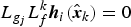
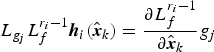
(8)where r i satisfies$$\eqalign{ &{\bi {F}}_{k}={\partial {\bi {f}} \over \partial {\bi {x}}}|_{x=\hat{x}_{k}},\quad {\bi {H}}_{k}={\partial {\bi {h}} \over \partial {\bi {x}}}|_{x=\hat{x}_{k}},\quad {\bi {A}}=(|{\bi {e}}_{y_{k+1/k}}|+\gamma|{\bi {e}}_{y_{k}}|) \cr &{\bi {N}}(\hat{{\bi {x}}}_{k})={\bi {g}}(\hat{{\bi {x}}}_{k})\{{\bi {U}}[\hat{{\bi {x}}}_{k}]\}^{-1},\quad {\bi {Z}}_{i}[\hat{{\bi {x}}}_{k}]=\sum_{l=1}^{r_i}{1 \over l!}L_{f}^{l}({\bi {h}}_{i}),\quad i=1,2,\cdots,m \cr &{\bi {U}}_{ij}[\hat{{\bi {x}}}_{k}]=L_{g_{j}}L_{f}^{r_i-1}{\bi {h}}_{i}[\hat{{\bi {x}}}_{k}],\quad i=1,2,\cdots,m,\quad j=1,2,\cdots,p }$$$L_{g_{j}}L_{f}^{k}{\bi {h}}_{i}(\hat{{\bi {x}}}_{k})=0$, where $i=1,2,\cdots,m,\ j=1,2,\cdots p$, and k i′ < r i−1, and $L_{g_{j}}L_{f}^{r_{i}-1}{\bi {h}}_{i}(\hat{{\bi {x}}}_{k})={\partial L_{f}^{r_{i}-1} \over \partial \hat{{\bi {x}}}_{k}}g_{j}$, where i = 1, 2,···, m and j = 1, 2,···p, are not all identically zero, which is the lowest order of the derivative of ${\bi {h}}_{i}(\hat{{\bi {x}}}_{k})$ in which any component of dk first appears arising from a successive differentiation and substitution for x i on the right hand side of Equation (6). Note that {ri} can also be interpreted as the set of the relative degrees of the system.
(2) The second step is to update the state estimate. We choose the boundary layer by comparing the adaptive boundary layer ψk+1 with the limit boundary layer ψlim it.
If ψk+1 < ψlim it holds good:
(9)$$\eqalign{ &\hat{{\bi {x}}}_{k+1/k}={\bi {f}}(\hat{{\bi {x}}}_{k}) \cr &\hat{{\bi {x}}}_{k+1}=\hat{{\bi {x}}}_{k+1/k}+{\bi {K}}_{k+1}{\bi {e}}_{y_{k+1/k}} \cr &{\bi {K}}_{k+1}={\bi {g}}(\hat{{\bi {x}}}_{k})\{{\bi {U}}[\hat{{\bi {x}}}_{k}]\}^{-1}\ {\it diag}\ [{\bi {A}} \bullet {sat}({\bi {e}}_{y_{k+1/k}},\hat{\bi {\psi}}_{k+1})][{diag}({\bi {e}}_{y_{k+1/k}})]^{-1} \cr &{\bi {A}}=(|{\bi {e}}_{y_{k+1/k}}|+\gamma|{\bi {e}}_{y_{k}}|)}$$If ψk+1 > ψlim it holds good:
(10)where$$\eqalign{ &\hat{{\bi {x}}}_{k+1/k}={\bi {f}}(\hat{{\bi {x}}}_{k}) \cr &\hat{{\bi {x}}}_{k+1}=\hat{{\bi {x}}}_{k+1/k}+{\bi {K}}_{k+1}{\bi {e}}_{y_{k+1/k}} \cr &{\bi {K}}_{k+1}={\bi {g}}(\hat{{\bi {x}}}_{k})\{{\bi {U}}[\hat{{\bi {x}}}_{k}]\}^{-1}\ {\it diag}\ [{\bi {A}}\bullet {sat}({\bi {e}}_{y_{k+1/k}},{\bi \psi}_{\lim it})][{diag}({\bi {e}}_{y_{k+1/k}})]^{-1} \cr &{\bi {A}}=(|{\bi {e}}_{y_{k+1/k}}|+\gamma|{\bi {e}}_{y_{k}}|)}$$$\hat{{\bi {x}}}_{k+1/k}$ and $\hat{{\bi {x}}}_{k+1}$ are the a priori and a posteriori estimation state and Kk+1 is the gain matrix of the APVSF. “sat” is a vector of the saturation function, defined as follows
(11)$$\eqalign{ sat ({\bi {e}}_{y_{k+1/k}},\psi)&=[sat(e_{y1_{k+1/k}},\psi_{1})\cdots\cdots {\it sat} (e_{yn_{k+1/k}},\psi_{n})]^{T} \cr sat (e_{yi_{k+1/k}},\psi_{i})&=\left\{ \matrix{ e_{yi_{k+1/k}}/\psi_{i},\ e_{yi_{k+1/k}}\leq\psi_{i} \hfill \cr sign (e_{yi_{k+1/k}}),\ e_{yi_{k+1/k}}\geq\psi_{i} }\right.}$$(3) The third step is to update the covariance.
(12)It can be noted that the state estimation update in Equations (9) and (10) needs to adopt the numerical integral method. The algorithm process of APVSF is the basis for the further development of ST-SP-PVSF. More details can be found in Cao et al. (Reference Cao, Li, Han and Li2016).$${\bi {P}}_{k+1}=({\bi {I}}-{\bi {K}}_{k+1}{\bi {H}}_{k+1}){\bi {P}}_{k+1/k}({\bi {I}}-{\bi {K}}_{k+1}{\bi {H}}_{k+1})^{T}+{\bi {K}}_{k+1}{\bi {R}}_{k+1}{\bi {K}}_{k+1}^{T}$$







3. STRONG TRACKING SIGMA-POINT PREDICTIVE VARIABLE STRUCTURE FILTER
In this section, the derivation of ST-SP-PVSF can be divided into three subsections. The first part is to introduce the sequence orthogonal principle into the APVSF for the improvement of robustness, which can also overcome the constraint of choosing the limit boundary layer ψlim it. Then, several sigma-point sampling strategies are employed to extend the above algorithm, such as the Unscented Transform (UT) strategy, cubature rule and Stirling's polynomial interpolation, which can enhance the estimate precision by capturing the second central moment's information on the model errors. Finally, the complete algorithm process of the ST-SP-PVSF is given and then used for the simulations in Section 4.
3.1. The design of sequence orthogonal principle
The mathematical expression of the sequence orthogonal principle is as follows (Zhou et al., Reference Zhou, Sun and Xi1993)
 $$\eqalign{ E({\bi \varepsilon}_{k+j}{\bi \varepsilon}_{k}^{T})&=0,\quad k=1,2,\cdots, \enspace j=1,2,\cdots \cr {\bi \varepsilon}_{k}&={\bi {y}}_{k}-\hat{{\bi {y}}}_{k/k-1} }$$
Any estimation errors can be shown in the output residual sequence εk. Then, the output residual is used to adjust the gain matrix by satisfying Equation (13), to orthogonalise all the output residuals for better accuracy.
The sequence orthogonal principle is applied by introducing the fading factors into the a priori state error covariance, which can weaken the effects of old observations and enhance the efficiency of new observations to improve the filtering robustness. Thus, the a priori state error covariance with the fading factor is updated as
 $${\bi {P}}_{k+1/k}={\bf \lambda}_{k+1}{\bi {F}}_{k}{\bi {P}}_{k}{\bi {F}}_{k}^{T}+{\bi {Q}}_{k}$$
where  ${\bf \lambda}_{k+1}=diag[\lambda_{k+1}^{1},\lambda_{k+1}^{2},\cdots,\lambda_{k+1}^{n}]$ is the multiple fading factor matrix and
 $\lambda_{k+1}^{i}\geq 1(i=1,2,\cdots,n)$ is the single fading factor which coincides with the different state variables. Qk is the positive definite symmetric matrix of white Gaussian process noise.
If the condition  ${\rm O}[|\tilde{{\bi {x}}}_{k}|^{2}]\leq {\rm O}[|\tilde{{\bi {x}}}_{k}|]$ is satisfied, then the following equation holds for the residual series
 $$\eqalign{ & E({\bi \varepsilon}_{k+j}{\bi \varepsilon}_{k}^{T})\approx {\bi {H}}_{k+j}{\bi {F}}_{k+j,k+j-1}({\bi {I}}-{\bi {K}}_{k+j-1}{\bi {H}}_{k+j-1})\bullet \cdots \cr &\bullet {\bi {F}}_{k+3,k+2}({\bi {I}}-{\bi {K}}_{k+2}{\bi {H}}_{k+2}){\bi {F}}_{k+2,k+1}({\bi {I}}-{\bi {K}}_{k+1}{\bi {H}}_{k+1}){\bi {F}}_{k+1,k}E[({\bi {x}}_{k}-\hat{{\bi {x}}}_{k}){\bi \varepsilon}_{k}^{T}] }$$
The estimate errors of system state and measurement can be described as
 $$\eqalign{ {\bi {x}}_{k+1}-\hat{{\bi {x}}}_{k+1}&={\bi {x}}_{k+1}-\hat{{\bi {x}}}_{k+1/k}-{\bi {K}}_{k+1}{\bi \varepsilon}_{k+1}=\tilde{{\bi {x}}}_{k+1/k}-{\bi {K}}_{k+1}{\bi \varepsilon}_{k+1} \cr {\bi \varepsilon}_{k+1}&={\bi {y}}_{k+1}-\hat{{\bi {y}}}_{k+1/k}={\bi {H}}_{k+1}\hat{{\bi {x}}}_{k+1/k}+{\bi {v}}_{k+1} }$$
Substitution of Equation (16) into Equation (15) and rearranging the terms, yields an equation with the assumption that  $\tilde{{\bi {x}}}_{k+1/k}$ is uncorrelated with
 ${\bi {v}}_{k}$, as follows
 $$\eqalign{ E[({\bi {x}}_{k+1}-\hat{{\bi {x}}}_{k+1}){\bi \varepsilon}_{k+1}^{T}]&=E[(\tilde{{\bi {x}}}_{k+1/k}-{\bi {K}}_{k+1}{\bi \varepsilon}_{k+1}){\bi \varepsilon}_{k+1}^{T}] \cr &=E[\tilde{{\bi {x}}}_{k+1/k}({\bi {H}}_{k+1}\hat{{\bi {x}}}_{k+1/k}+{\bi {v}}_{k+1})^{T}]-{\bi {K}}_{k+1}E[{\bi \varepsilon}_{k+1}{\bi \varepsilon}_{k+1}^{T}] \cr &={\bi {P}}_{k+1/k}{\bi {H}}_{k+1}^{T}-{\bi {K}}_{k+1}{\bi {V}}_{k+1} \cr {\bi {V}}_{k+1}&=E({\bi \varepsilon}_{k+1}{\bi \varepsilon}_{k+1}^{T}) }$$
Considering the sequence orthogonal principle in Equation (13), the above sufficient condition can be formulated as
 $$E[({\bi {x}}_{k+1}-\hat{{\bi {x}}}_{k+1}){\bi \varepsilon}_{k+1}^{T}]={\bi {P}}_{k+1/k}{\bi {H}}_{k+1}^{T}-{\bi {K}}_{k+1}{\bi {V}}_{k+1}=0$$
It is obvious that if the uncertainty model errors, perturbations or estimation errors exist, their impact effects will be projected into the residuals εk+1, which will be exhibited in Vk+1 to break the equivalence in Equation (13). In the other words, the output residual sequence is not orthogonal. Therefore, the multiple fading factor matrix is introduced to adjust the gain matrix Kk+1 to satisfy Equation (13). Another expression of gain matrix Kk+1 in APVSF is given here for further derivation when the smoothing boundary layer relationship ψk+1 ≤ ψlim it is satisfied:
 $${\bi {K}}_{k+1}={\bi {N}}\bullet \overline{A}\bullet{\bi \psi}_{k+1}^{-1}={\bi {P}}_{k+1/k}{\bi {H}}_{k+1}^{T}({\bi {H}}_{k+1}{\bi {P}}_{k+1/k}{\bi {H}}_{k+1}^{T}+{\bi {R}}_{k+1})^{-1}$$
inserting this into Equation (18) and rearranging the terms as follows yields
 $$\eqalign{ {\bi {P}}_{k+1/k}{\bi {H}}_{k+1}^{T}-{\bi {P}}_{k+1/k}{\bi {H}}_{k+1}^{T}({\bi {H}}_{k+1}{\bi {P}}_{k+1/k}{\bi {H}}_{k+1}^{T}+{\bi {R}}_{k+1})^{-1}{\bi {V}}_{k+1} \cr ={\bi {P}}_{k+1/k}{\bi {H}}_{k+1}^{T}({\bi {I}}-({\bi {H}}_{k+1}{\bi {P}}_{k+1/k}{\bi {H}}_{k+1}^{T}+{\bi {R}}_{k+1})^{-1}{\bi {V}}_{k+1})=0 }$$
Thus, another equivalent condition of Equation (18) can be derived as
 $${\bi {I}}-({\bi {H}}_{k+1}{\bi {P}}_{k+1/k}{\bi {H}}_{k+1}^{T}+{\bi {R}}_{k+1})^{-1}{\bi {V}}_{k+1}=0$$
Then, the a priori state error covariance with the fading factor Equation (14) can be substituted into the above equation.
 $${\bi {H}}_{k+l}{\bi \lambda}_{k+l}{\bi {F}}_{k}{\bi {P}}_{k}{\bi {F}}_{k}^{T}{\bi {H}}_{k+l}^{T} ={\bi {V}}_{k+1}-{\bi {R}}_{k+1}-{\bi {H}}_{k+1}{\bi {Q}}_{k}{\bi {H}}_{k+1}^{T}$$
In order to avoid the serious regulating effect of a fading factor, the weakening factor β is introduced into Equation (22) to smooth the state estimation, as
 $${\bi {H}}_{k+l}{\bi \lambda}_{k+1}{\bi {F}}_{k}{\bi {P}}_{k}{\bi {F}}_{k}^{T}{\bi {H}}_{k+1}^{T}\ ={\bi {V}}_{k+1}-\beta {\bi {R}}_{k+1}-{\bi {H}}_{k+1}{\bi {Q}}_{k}{\bi {H}}_{k+1}^{T}$$
The weakening factor needs to satisfy β ≥ 1, which can be chosen by experience or calculated by using the following rule
 $$\beta=\min\left(\sum_{k=1}^L\sum_{i=1}^n|{\bi {x}}_{i,k}-\hat{{\bi {x}}}_{i,k}|\right)$$
where L is the number of simulation steps. It can reflect the cumulative errors in the filtering process.
Then, to calculate the trace on the both sides of the Equation (23) and rearranging the terms, yields equations as follows
 $$\eqalign{ &tr[{\bi \lambda}_{k+1}{\bi {M}}_{k+1}]=tr[{\bi {N}}_{k+1}] \cr &{\bi {N}}_{k+1}={\bi {V}}_{k+1}-\beta {\bi {R}}_{k+1}-{\bi {H}}_{k+1}{\bi {Q}}_{k}{\bi {H}}_{k+1}^{T} \cr &{\bi {M}}_{k+1}={\bi {F}}_{k}{\bi {P}}_{k}{\bi {F}}_{k}^{T}{\bi {H}}_{k+1}^{T}{\bi {H}}_{k+1} }$$
According to the prior knowledge of the object, the proportional relationship between the multiple fading factors can be designed as
 $$\eqalign{ &\lambda_{k+1}^{1}:\lambda_{k+1}^{2}:\cdots:\lambda_{k+1}^{n}=\alpha_{1}:\alpha_{2}:\cdots:\alpha_{n} \cr &\lambda_{k+1}^{i}=\alpha_{i}c_{k+1},\ i=1,2,\cdots,n }$$
where αi ≥ 1 is a constant chosen based on experience. c k+1 is an undetermined factor. Hence, the general algorithm of the multiple fading factors can be designed as
 $$\lambda_{k+1}^{i}= \left\{ \matrix{ \alpha_{i}c_{k+1}, &\alpha_{i}c_{k+1}>1 \cr 1 \hfill&\alpha_{i}c_{k+1}\leq 1 }\right.$$
inserting into Equation (25), we can obtain the expanding expression as
 $$\eqalign{ tr[{\bi \lambda}_{k+1}{\bi {M}}_{k+1}]&=tr\left\{\left[\matrix{ \lambda_{k+1}^{1} & 0 & \cdots & 0 \cr 0 & \lambda_{k+1}^{2} & \cdots & 0 \cr \vdots &\vdots &\ddots & \vdots \cr 0 & 0 & \cdots & \lambda_{k+1}^{n} }\right]{\bi {M}}_{k+1}\right\} \cr &=tr\left\{\left[\matrix{ \alpha_{1}c_{k+1} & 0 & \cdots & 0 \cr 0 & \alpha_{2}c_{k+1} & \cdots & 0 \cr \vdots &\vdots &\ddots & \vdots \cr 0 & 0 & \cdots & \alpha_{n}c_{k+1} }\right]{\bi {M}}_{k+1}\right\}=tr[{\bi {N}}_{k+1}] }$$
Therefore, the undetermined factor c k+1 can be computed as
 $$c_{k+1}={tr[{\bi {N}}_{k+1}] \over \sum^n_{i=1}\alpha_i{\bi {M}}^{ii}_{k+1}}$$
Additionally, the actual values of residual matrix Vk+1 cannot be obtained directly, and they need to be estimated using the following formula
 $${\bi V}_{k+1}= \left\{ \matrix{ {\bi \varepsilon}_1{\bi \varepsilon}^{T}_1 \hfill & k=1 \cr {\rho{\bi {V}}_{k}+{\bi \varepsilon}_{k}{\bi \varepsilon}_{k}^{T} \over 1+\rho}, & k\geq 2} \right.$$
The parameter ρ is the forgetting factor with a limitation of 0 < ρ ≤ 1, and is usually set to 0.95. Until now, the orthogonal sequence principle has been applied to the APVSF, which plays an important role in adjusting the gain matrix in order to satisfy Equation (13).
3.2. The extension of the sigma-point sampling strategy
On the basis of the above, several sigma-point sampling strategies have been used to extend the above filter algorithm, such as the UT strategy (Julier and Uhlmann, Reference Julier and Uhlmann2000), cubature rule (Arasaratnam and Haykin, Reference Arasaratnam and Haykin2009) and Stirling's polynomial interpolation (Norgaard et al., Reference Norgaard, Poulsen and Ravn2000). For simplicity, this part is derived in the general form, but in the process of application, the different sampling strategies can be used or replaced. Before the introduction of the fading factor, all the covariances are given with the symbol “′”. Therefore, the a priori state error covariance  ${\bi {P}}_{k+1/k}^{\prime}$, the a priori measurement error covariance
 ${\bi {P}}_{yy, k+1}^{\prime}$ and the cross covariance
 ${\bi {P}}_{xy,k+1}^{\prime}$ are expressed as
 $$\eqalign{ {\bi {P}}_{k+1/k}^{\prime}&=E\{[{\bi {x}}_{k+1}-\hat{{\bi {x}}}_{k+1/k}][{\bi {x}}_{k+1}-\hat{{\bi {x}}}_{k+1/k}]^{T}\} \cr {\bi {P}}_{yy, k+1}^\prime &=E\{[{\bi {y}}_{k+1}-\hat{{\bi {y}}}_{k+1/k}][{\bi {y}}_{k+1}-\hat{{\bi {y}}}_{k+1/k}]^{T}\} \cr {\bi {P}}_{xy,k+1}^\prime&=E\{[{\bi {x}}_{k+1}-\hat{{\bi {x}}}_{k+1/k}][{\bi {y}}_{k+1}-\hat{{\bi {y}}}_{k+1/k}]^{T}\} \cr {\bi {P}}_{k+1/k}^\prime &={\bi {F}}_{k}{\bi {P}}_{k}{\bi {F}}_{k}^{T}+{\bi {Q}}_{k} }$$
According to the assumption in Equation (6),  $\tilde{{\bi {x}}}_{k+1/k}$ is uncorrelated with vk, and the covariance
 ${\bi {P}}_{yy, k+1}^{\prime}$ and
 ${\bi {P}}_{xy,k+1}^{\prime}$ can be expressed, respectively as
 $$\eqalign{ {\bi {P}}_{yy, k+1}^\prime &=E\{[{\bi {y}}_{k+1}-\hat{{\bi {y}}}_{k+1/k}][{\bi {y}}_{k+1}-\hat{{\bi {y}}}_{k+1/k}]^{T}\} \cr &=E\{[{\bi {H}}_{k+1}({\bi {x}}_{k+1}-\hat{{\bi {x}}}_{k+1/k})+{\bi {v}}_{k+1}][{\bi {H}}_{k+1}({\bi {x}}_{k+1}-\hat{{\bi {x}}}_{k+1/k})+{\bi {v}}_{k+1}]^{T}\} \cr &={\bi {H}}_{k+1}E\{[{\bi {x}}_{k+1}-\hat{{\bi {x}}}_{k+1/k}][{\bi {x}}_{k+1}-\hat{{\bi {x}}}_{k+1/k}]^{T}\}{\bi {H}}_{k+1}^{T}+E[{\bi {v}}_{k+1}{\bi {v}}_{k+1}^{T}] \cr &={\bi {H}}_{k+1}{\bi {P}}_{k+1/k}^\prime {\bi {H}}_{k+1}^{T}+{\bi {R}}_{k+1} }$$
 $$\eqalign{ P_{\eta,k+1}^{\prime}&=E\{[{\bi {x}}_{k+1}-\hat{{\bi {x}}}_{k+1/k}][{\bi {y}}_{k+1}-\hat{{\bi {y}}}_{k+1/k}]^{T}\} \cr &=E\{[{\bi {x}}_{k+1}-\hat{{\bi {x}}}_{k+1/k}][{\bi {H}}_{k+1}({\bi {x}}_{k+1}-\hat{{\bi {x}}}_{k+1/k})+{\bi {v}}_{k+1}]^{T}\} \cr &={\bi {P}}_{k+1/k}^\prime {\bi {H}}_{k+1}^{T} }$$
If Pk+1/k stands for the a priori state error covariance with the fading factor λk+1, the matrix  ${\bi {P}}_{k+1/k}^{\prime} $ can instead be
 ${\bi {P}}_{k+1/k}$ and the relevant covariance can be redefined as
 $$\eqalign{ {\bi {P}}_{yy, k+1}&={\bi {H}}_{k+1}{\bi {P}}_{k+1/k}{\bi {H}}_{k+1}^{T}+{\bi {R}}_{k+1} \cr {\bi {P}}_{xy, k+1}&={\bi {P}}_{k+1/k}{\bi {H}}_{k+1}^{T} }$$
This is because the Rk+1 is the positive definite symmetric matrix; thus, the covariance matrices Pk+1/k and  ${\bi {P}}_{k+1/k}^{\prime} $ can be inverted. In addition, the Jacobian matrix of measurement equation Hk+1 cannot be propagated by sigma-points, which can be replaced by the equivalent matrices of covariance matrices Pk+1/k and
 ${\bi {P}}_{k+1/k}^{\prime}$. Therefore, Hk+1 can be redefined as
 $$\eqalign{ {\bi {H}}_{k+1}&=[{\bi {P}}_{xy, k+1}^\prime]^{T}[{\bi {P}}_{k+1/k}^\prime]^{-1} \cr {\bi {H}}_{k+1}&=[{\bi {P}}_{xy, k+1}]^{T}[{\bi {P}}_{k+1/k}]^{-1} }$$
We then substitute Equations (34) and (35) into Equations (12) and (19), and rearrange all the terms. The adjusted gain matrix Kk+1 and the a posteriori state error covariance Pk+1 can be equivalently expressed as
 $$\eqalign{ {\bi {K}}_{k+1}&={\bi {P}}_{xy,k+1}{\bi {P}}_{yy, k+1}^{-1} \cr {\bi {P}}_{k+1}&={\bi {P}}_{k+1/k}-{\bi {K}}_{k+1}{\bi {P}}_{k+1/k}{\bi {K}}_{k+1}^{T} }$$
Similarly, the matrices Nk+1 and Mk+1 can be updated with respect to the above results as
 $$\eqalign{ {\bi {N}}_{k+1}&={\bi {V}}_{k+1}-{\bi {R}}_{k+1}-[{\bi {P}}_{xy,k+1}^\prime]^{T}[{\bi {P}}_{k+1/k}^\prime]^{-1}{\bi {Q}}_{k}[{\bi {P}}_{k+1/k}^\prime]^{-1}[{\bi {P}}_{xy,k+1}^\prime]\cr {\bi {M}}_{k+1}&={\bi {F}}_{k}{\bi {P}}_{k}{\bi {F}}_{k}^{T}{\bi {H}}_{k+1}^{T}{\bi {H}}_{k+1}={\bi {H}}_{k+1}[{\bi {P}}_{k+1/k}^\prime-{\bi {Q}}_{k}]{\bi {H}}_{k+1}^{T}\cr &={\bi {H}}_{k+1}{\bi {P}}_{k+1/k}^\prime {\bi {H}}_{k+1}^{T}-{\bi {H}}_{k+1}{\bi {Q}}_{k}{\bi {H}}_{k+1}^{T}={\bi {H}}_{k+1}{\bi {P}}_{k+1/k}^\prime {\bi {H}}_{k+1}^{T}+{\bi {R}}_{k+1}-{\bi {V}}_{k+1}+{\bi {N}}_{k+1}\cr &={\bi {P}}_{yy, k+1}^\prime -{\bi {V}}_{k+1}+{\bi {N}}_{k+1} }$$
Now, all the variable matrices can be calculated and propagated by the different kinds of covariance or gain matrices, which are prepared for the extension by the sigma points. This is because all the covariances can be computed from the sigma points.
3.3. The algorithm process of ST-SP-PVS
Based on the above work, the orthogonal sequence principle is successfully applied to improve the APVSF with the ability for strong tracking of the residual estimate errors. Then, the improved method is extended by the sigma-point strategies for second order estimation precision. This novel filtering methodology is named Strong Tracking Sigma-Point Predictive Variable Structure Filter (ST-SP-PVSF), and can directly show its technical characteristics. Additionally, it is significant to emphasise the sigma-point sampling strategy. Any sampling strategies that calculate the covariance to propagate the variables can be adopted to extend and be used in the ST-SP-PVSF.
In this subsection, the cubature rule is employed to implement the ST-SP-PVSF algorithm process as an example. The other sampling strategies (UT strategy or Stirling's polynomial interpolation) can also be used in a similar way. With respect to the above achievements and discussions, the filtering algorithm for ST-SP-PVSF can be described as follows
(1) The first step is to set the initial values and chose the sigma points.
(38)$$\left\{ \matrix{ \hat{{\bi {x}}}_{0}=E({\bi {x}}_{0})\hfill \cr {\bi {P}}_{x,0}=Var({\bi {x}}_{0})=E[({\bi {x}}_{0}-\hat{{\bi {x}}}_{0})({\bi {x}}_{0}-\hat{{\bi {x}}}_{0})^{T}] }\right.$$

The cubature rule is used to calculate the sigma points, which can be generated through the use of  $(\hat{{\bi {x}}}_{k},{\bi {P}}_{x,k})$ by the Cholesky decomposition method.
 $$\eqalign{ {\bi {P}}_{xk}&=S_{k}S_{k}^{T}\cr & S_{k}=[\matrix{ \sigma_{k1} &\sigma_{k2} &\cdots &\sigma_{kn}}] }$$
The relevant sigma points are expressed as
 $$\left\{ \matrix{ \xi_{i,k}=\hat{{\bi {x}}}_{k}+\sqrt{n}\sigma_{k_i}=\hat{{\bi {x}}}_{k}+\hat{\sigma}_{k_i}\hfill \cr \xi_{i+n,k}=\hat{x}_{k}-\sqrt{n}\sigma_{k_i}=\hat{{\bi {x}}}_{k}-\hat{\sigma}_{k_i}} \right. \quad , i=1,2,\cdots,n$$
(2) The second step is the time update. Each sigma-point ξik(i = 1, ···, 2n) is propagated through the nonlinear function of f(•) to generate the a priori state estimate
$\hat{{\bi {x}}}_{k+1/k}$ with the a priori state error covariance ${\bi {P}}_{k+1/k}^{\prime} $ without the fading factor, as
(41)According the design of ST-SP-PVSF, a multiple fading factor matrix is introduced into the above equation. The updated a priori state error covariance is given as$$\eqalign{ \hat{{\bi {x}}}_{i,k+1/k}&={\bi {f}}(\xi_{i,k}),\quad \hat{{\bi {x}}}_{k+1/k}=\sum_{i=1}^{2n}W_{i}^{m}\hat{{\bi {x}}}_{i,k+1/k}\cr {\bi {P}}_{k+1/k}^\prime &=\sum_{i=1}^{2n}W_{i}^{m}(\hat{{\bi {x}}}_{i,k+1/k}-\hat{{\bi {x}}}_{k+1/k})(\hat{{\bi {x}}}_{i,k+1/k}-\hat{{\bi {x}}}_{k+1/k})^{T}+{\bi {Q}}_{k} }$$(42)$${\bi {P}}_{k+1/k}={\bi \lambda}_{k+1}\sum_{i=1}^{2n}W_{i}^{m}(\hat{{\bi {x}}}_{i,k+1/k}-\hat{{\bi {x}}}_{k+1/k})(\hat{{\bi {x}}}_{i,k+1/k}-\hat{{\bi {x}}}_{k+1/k})^{T}+{\bi {Q}}_{k}$$(3) The third step is to calculate the multiple fading factor matrix. Utilising the a priori state estimate and error covariance
$(\hat{{\bi {x}}}_{k+1/k},{\bi {P}}_{k+1/k}^{\prime})$ to generate the new sigma points $\hat{x}_{i,k+1/k}^{\prime} (i=1,\cdots,2n)$. The relevant measurement error covariance and cross covariance can be expressed as
(43)Then, the multiple fading factor matrix λk+1 can be computed as$$\eqalign{ \hat{{\bi {y}}}_{i,k+1/k}^\prime &={\bi {h}}(\hat{{\bi {x}}}_{i,k+1/k}^{\prime}),\quad \hat{{\bi {y}}}_{k+1/k}^\prime =\sum_{i=1}^{2n}W_{i}^{m}\hat{{\bi {y}}}_{i,k+1/k}^\prime \cr {\bi {P}}_{yy,k+1}^\prime&=\sum_{i=1}^{2n}W_{i}^{m}(\hat{{\bi {y}}}_{i,k+1/k}^\prime -\hat{y}_{k+1/k}^\prime)(\hat{{\bi {y}}}_{i,k+1/k}^\prime -\hat{{\bi {y}}}_{k+1/k}^\prime)^{T}+{\bi {R}}_{k+1}\cr {\bi {P}}_{xy,k+1}^\prime&=\sum_{i=1}^{2n}W_{i}^{m}(\hat{{\bi {x}}}_{i,k+1/k}^\prime -\hat{{\bi {x}}}_{k+1/k}^\prime)(\hat{{\bi {y}}}_{i,k+1/k}^\prime -\hat{{\bi {y}}}_{k+1/k}^\prime)^{T} }$$(44)$$\eqalign{ &{\bi \lambda}_{k+1}=diag[\lambda_{k+1}^{1}\quad \lambda_{k+1}^{2}\quad \cdots\quad \lambda_{k+1}^{n}] \cr &\lambda_{k+1}^{i}= \left\{ \matrix{ \alpha_{i}c_{k+1}\cr 1 }, \matrix{ \alpha_{i}c_{k+1}>1 \cr \alpha_{i}c_{k+1}\leq 1 } \quad c_{k+1}={tr[{\bi {N}}_{k+1}] \over \sum_{i=1}^n\alpha_{i}M_{k+1}^{ii}} \right. \cr &{\bi {N}}_{k+1}={\bi {V}}_{k+1}-{\bi {R}}_{k+1}-[{\bi {P}}_{xy,k+1}^\prime]^{T}[{\bi {P}}_{k+1/k}^\prime ]^{-1}{\bi {Q}}_{k}[{\bi {P}}_{k+1/k}^\prime ]^{-1}[{\bi {P}}_{xy,k+1}^\prime ]\cr &{\bi {M}}_{k+1}={\bi {P}}_{yy, k+1}^\prime -{\bi {V}}_{k+1}+{\bi {N}}_{k+1}\cr &{\bi {V}}_{k+1}= \left\{ \matrix{ {\bi \varepsilon}_{1}{\bi \varepsilon}_{1}^{T} \cr {\rho{\bi {V}}_{k}+{\bi \varepsilon}_{k+1}{\bi \varepsilon}_{k+1}^{T} \over 1+\rho} }, \quad \matrix{ k=1 \cr k\geq 2 } \right.}$$(4) The fourth step is to update the state estimate. The new set of sigma points
$\hat{{\bi {x}}}_{i,k+1/k}(i=1,\cdots,2n)$ can also be computed by $(\hat{{\bi {x}}}_{k+1/k},{\bi {P}}_{k+1/k})$, which can be used to update the gain matrix and the system state variables.
(45)It is obvious that the limit boundary layer ψlim it is not necessary when compared with the APVSF. Then, the final posterior state estimate and covariance can be propagated as$$\eqalign{ {\bi \psi}_{i,k+1}&=(\overline{{\bi A}}_{i}^{-1}{\bi N}_{i}^{-1}{\bi {P}}_{k+1/k}{\bi {H}}_{i,k+1}^{T}{\bi {S}}_{i,k+1}^{-1})^{-1},\quad {\bi {S}}_{i,k+1}={\bi {H}}_{i,k+1}{\bi {P}}_{k+1/k}{\bi {H}}_{i,k+1}^T +{\bi {R}}_{k+1} \cr {\bi {K}}_{i,k+1}&={\bi {N}}_{i}\overline{{\bi {A}}}_{i}\hat{{\bi \psi}}^{-1}_{i,k+1},\quad {\bi {e}}_{y_{i,k+1/k}}={\bi {y}}_{k+1}-\hat{{\bi {y}}}_{k_i},\ -{\bi {Z}}[\hat{{\bi {x}}}_{i,k+1/k}]\cr \hat{{\bi {x}}}_{i,k+1/k+1}&=\hat{{\bi {x}}}_{i,k+1/k}+{\bi {K}}_{i,k+1}{\bi {e}}_{y_{i,k+1/k}} }$$(46)$$\eqalign{ \hat{{\bi {x}}}_{k+1}&=\sum_{i=1}^{2n}W_{i}^{m} \hat{{\bi {x}}}_{i,k+1/k+1}\cr {\bi {P}}_{k+1}&=\sum_{i=1}^{2n}W_{i}^{m}(\hat{{\bi {x}}}_{i,k+1/k+1}-\hat{{\bi {x}}}_{k+1})(\hat{{\bi {x}}}_{i,k+1/k+1}-\hat{{\bi {x}}}_{k+1})^{T} }$$










The recursive filtering algorithm for the ST-SP-PVSF is completely designed above, and is used for numerical simulation in the following section.
4. NUMERICAL SIMULATIONS
In this section, the proposed ST-SP-PVSF is simulated to evaluate its performance compared with the APVSF for attitude synchronisation estimation in the SFF. Another comparison is also given with the traditional Unscented Kalman Filter (UKF), which is in widespread use in many fields with excellent filtering performance. Note that the simulation figures of the attitude and the angular velocity are all error graphs of the actual values and the estimated values.
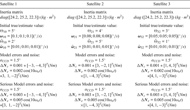
The numerical simulation conditions are as follows: the relative attitude is assumed to be described by  ${\bi {q}}=[\cos{\Theta \over 2}\quad {\sqrt{3} \over 3}\sin{\Theta \over 2}\quad {\sqrt{3} \over 3}\sin{\Theta \over 2}\quad {\sqrt{3} \over 3}\sin{\Theta \over 2}]^{T}$, the mean square of measurement noise is represented by σCCD with Gaussian white noise. The actual model error of this system is assumed to be composed of d = ΔNc+ΔNe and it is assumed that ΔNc is the constant component and ΔNe is the periodic component. The period angular velocity of the model error is ωo = 0.066°/s, and the sampling interval is set as Δt = 0.5s. In addition, it is assumed that the satellite formation consists of small satellites and the unit of the y-axis is degrees or degrees per second in all the simulation figures, respectively.The simulation parameters are given in Table 1.
System simulation parameters.

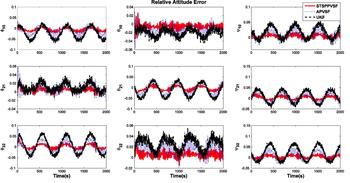
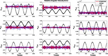
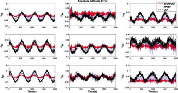
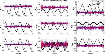
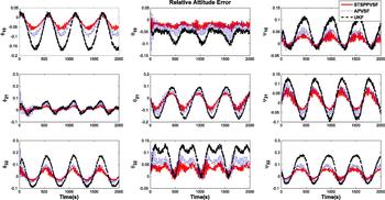
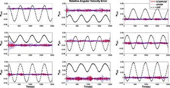
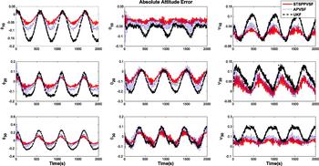
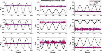
In this section, the ST-SP-PVSF, the APVSF and the UKF are compared with simulation results depicted in Figures 1–4, which show the relative/absolute attitude and angular velocity estimate errors in the synchronisation process for SFF. It is obvious that the three types of filters have similar estimate trends for the attitude estimation accuracy in Figure 1 and Figure 3. However, the proposed method and APVSF have better accuracy than the traditional UKF. It can be seen that the ST-SP-PVSF is more stable and converges faster to zero than the other two filters. From the relative/absolute angular velocity estimate results in Figures 2 and 4, the simulation results by using UKF have serious deviations and fluctuations, which are caused by the periodic model errors introduced into the simulation process. By contrast, the estimate errors of the ST-SP-PVSF and the APVSF converge to a small region around the true state trajectories without the obvious fluctuations. It is illustrated that these two methods have the ability to inhibit the unknown model errors by updating the modelling accuracy. In addition, the proposed ST-SP-PVSF is given with the theoretical advantages of the orthogonal sequence principle and sigma point strategy, which has the better performance in robustness and estimate accuracy than the APVSF. Furthermore, for the ST-SP-PVSF, it is unnecessary to choose the limit boundary layer when compared with the APVSF, which improves its autonomy and flexibility for applications in different fields.
Relative attitude estimation error.

Relative angular velocity estimation error.

Absolute attitude estimation error.

Absolute angular velocity estimation error.

Similarly, when we improve the level of the model errors, the simulation results (Figures 5–8) will show more significant differences between the proposed method and the traditional UKF. For serious model errors, especially when periodic model errors exist, the UKF has no ability to deal with such perturbations, which has obvious disadvantages compared with the proposed method. Of course, the ST-SP-PVSF still has the best filtering performance, which is also the aim of the theoretical research in this paper.
The estimation error of the relative attitude with serious model errors.

The estimation error of the relative angular velocity with serious model errors.

The estimation error of the absolute attitude with serious model errors.

The estimation error of the absolute angular velocity with serious model error.

5. CONCLUSIONS
In this paper, a mathematical model of attitude synchronisation and the APVSF algorithm were reviewed. Then, the orthogonal sequence principle was used to improve the traditional APVSF; on which basis, the sigma point sampling strategy is further employed to extend this method to propose the ST-SP-PVSF. It is shown that the proposed method has better robustness and eliminates the restriction of limit boundary layer. In addition, it can also capture the second central moment's information of the model errors, which can enhance the estimate precision compared with the APVSF. Finally, numerical comparisons with the classical UKF and APVSF have been included for attitude synchronisation estimation with the measurement noises and model errors, in order to verify the performance of the proposed ST-SP-PVSF.
ACKNOWLEDGMENTS
This research work was funded by the National Natural Science Foundation of China (no. 61503414 and no.11402257), the State Key Laboratory of Geo-information Engineering (no. SKLGIE2016-Z-3-l) and the State Key Laboratory of Astronautic Dynamics Foundation (ADL) (no. 2016ADL-DW0202). The authors express their gratitude to the editors and reviewers for their valuable comments that can help to enhance the quality of this paper.