





1. Introduction
Flow-induced vibration (FIV) is a critical problem in many fields and can lead to a wide range of consequences, both detrimental and beneficial. On the negative side, FIV can cause fatigue damage and even catastrophic structural failure in engineering systems such as bridges (Song et al. Reference Song, Kim, Kwon and Choi2022). Conversely, FIV is also exploited for energy harvesting (Bos & Wellens Reference Bos and Wellens2021; Ma & Zhou Reference Ma and Zhou2022) or flow sensing (Li et al. Reference Li, Fan, Li, He, Qiao, Shi, Yan, Liu, Liu and Sun2020).
Two well-known forms of FIV involving bluff bodies are vortex-induced vibration (VIV) and galloping (Blevins Reference Blevins1977; Naudascher & Rockwell Reference Naudascher and Rockwell2012). Vortex-induced vibration develops from the unsteady vortex shedding dynamics of the bluff body and occurs when the frequency of vortex shedding synchronises with the natural frequency of the system. Vortex-induced vibration is typically self-limiting, with the oscillation amplitude remaining of the order of the characteristic dimension of the bluff body. Galloping, on the other hand, arises when a small transverse motion of a non-circular bluff body generates aerodynamic forces that further amplify the motion. This can result in large-amplitude oscillations, with the amplitude typically increasing with flow velocity. An important parameter in characterising VIV and galloping is the reduced velocity
 $U_r$
, defined as
 $U_r = U_\infty /(f_0 d)$
, where
 $U_\infty$
is the free-stream velocity,
 $f_0$
is the natural frequency of the system and
 $d$
is a characteristic length of the bluff body. Reduced velocity serves as a non-dimensional measure of flow speed relative to the structural dynamics. It effectively indicates how significant vortex shedding unsteadiness is in influencing the structural response. Specifically, it compares the vortex shedding frequency, given by
 $f_{\textit{VS}} = St \, U_\infty / d$
(where
 $St$
is the Strouhal number of the considered bluff body), with the system’s natural frequency: unsteadiness is important for small values of the reduced velocity (typically
 $U_r\lt 20$
) while quasi-steady aerodynamics is expected to hold for large values of the reduced velocity. It therefore plays a crucial role in determining the onset and nature of oscillations. For instance, VIV typically manifests within a narrow band of reduced velocity, most commonly between 5 and 8 for two-dimensional bluff bodies (Blevins Reference Blevins1990). In contrast, galloping can occur over a much broader range of values of
 $U_r$
, with its onset dependent on the mass and damping characteristics of the system (Parkinson & Brooks Reference Parkinson and Brooks1961).
In many practical situations, FIV occurs in pendulum-like systems. Examples include underwater towed bodies (Buckham et al. Reference Buckham, Nahon, Seto, Zhao and Lambert2003), suspended loads lifted by helicopters (Oktay & Sultan Reference Oktay and Sultan2013), objects moved by towing cranes (Jin et al. Reference Jin, Liu, Zheng and Chen2020) and cable transport cabins (Myskiw et al. Reference Myskiw, Haffner, Paillé, Borée and Sicot2024). A large volume of studies have been dedicated to understanding the dynamic behaviour of such systems using simple geometries in fluid environments, particularly in water flow. In a two-dimensional (2-D) setting, Orchini et al. (Reference Orchini, Kellay and Mazzino2015) explored the dynamics of a rigid pendulum in a soap film flow and attributed the resulting oscillatory motion to galloping instability. The VIV of a positively buoyant, tethered 2-D circular cylinder has been studied through both numerical simulations (Ryan et al. Reference Ryan, Pregnalato, Thompson and Hourigan2004, Reference Ryan, Thompson and Hourigan2007) and experiments (Carberry & Sheridan Reference Carberry and Sheridan2007). These studies demonstrated an abrupt shift from in-line to transverse oscillations as the free-stream velocity increased. This phenomenon strongly depends on the mass ratio, defined as the ratio between the mass of the body and the mass of the displaced fluid. In three-dimensional (3-D) settings, the VIV behaviour of a tethered sphere is more complicated, driven by several distinct wake modes (Govardhan & Williamson Reference Govardhan and Williamson1997, Reference Govardhan and Williamson2005; Lee et al. Reference Lee, Hourigan and Thompson2013; Rajamuni et al. Reference Rajamuni, Thompson and Hourigan2020; Kovalev et al. Reference Kovalev, Eshbal and Van Hout2022).
When a pendulum system is coupled with air flow, it was found in Myskiw et al. (Reference Myskiw, Haffner, Paillé, Borée and Sicot2024) that a cube pendulum is potentially subject to galloping instability, over a range of static yaw angles. The stability of the system was found to be well predicted by the quasi-steady theory (Den Hartog Reference Den Hartog1932). At low reduced velocities, an unsteady phase delay between the wake and the pendulum dynamics was also identified. However, a prediction of the response of the pendulum system was not proposed, and the classical quasi-steady prediction method proposed by Parkinson & Brooks (Reference Parkinson and Brooks1961) – which assumes instantaneous force response – is not applicable in this context.
Based on the facilities and prior experience of our laboratory, we investigate the FIV of a pendulum system with one degree of freedom, free to oscillate in a plane perpendicular to the incoming air flow. The pendulum system consists of a thin square plate mounted at the free end, oriented normal to the incoming airflow, with a variable-length splitter plate attached downstream. The combined assembly is referred to here as a T-shaped body and is designed to trigger and study galloping. This configuration is inspired by prior studies on 2-D cylinders with splitter plates (Nakamura et al. Reference Nakamura, Hirata and Kashima1994; Assi & Bearman Reference Assi and Bearman2015).
While the set-up may appear somewhat unconventional, we believe that it represents the simplest geometry capable of generating galloping while enabling the exploration of a wide parametric space for systematic investigation. Using 3-D printing technology and miniature pressure sensors, we are able to measure the pressure distribution on the splitter plate – an aspect that, to the best of our knowledge, has not been previously addressed in similar set-ups, neither with static nor elastically mounted bluff bodies. This capability allows for a more detailed understanding of the underlying FIV mechanisms. Furthermore, the set-up holds potential for energy harvesting applications, especially in situations where usable space is limited, restricting the use of traditional devices such as wind turbines.
The paper is structured as follows: § 2 first details the wind tunnel, T-shaped pendulum arrangement and measurement methodology. Based on static measurements, the modelling of the pendulum dynamics, the prediction of its stability and the description of the wake dynamics are then presented in § 3. The general features of the experimental characterisation of the pendulum dynamics are subsequently detailed in § 4. The pendulum is shown to undergo galloping instability, and the amplitude and frequency of its oscillations are derived within the quasi-static framework. The aerodynamic forces acting on the pendulum are then examined in detail in § 5 to assess the validity of the quasi-static approach. This is followed by an investigation of the unsteady aerodynamic phenomena observed at low reduced velocities in § 6. A simplified model, based on a Van der Pol oscillator, is subsequently presented in § 7. Finally, concluding remarks are provided in § 8.
2. Experimental set-ups
2.1. Wind tunnel facility and model geometry
All experiments take place in a closed-loop wind tunnel at ENS de Lyon. The test section has a square cross-section of
 $51 \times 51$
cm
 $^2$
and extends 4 m in length. Under most operating conditions, the incoming flow has a turbulence intensity of 3 %. The geometry of the T-shaped body is shown in the isometric view in figure 1
 $(a)$
. The body consists of two rectangular plates perpendicular to each other: a thin square plate at the front and a splitter plate at the rear. The front plate is made from a 1 mm thick printed circuit board (PCB). The splitter plate is 3-D-printed with a thickness of 2.6 mm using acrylonitrile butadiene styrene-like photopolymer resin, which has a density of 1.1 g cm
 $^{-3}$
. The width (height) of the square plate is
 $d = 45$
mm. Two groups of experiments using the T-shaped body in the wind tunnel are conducted and detailed respectively in the next two subsections.
Schematics of the experimental set-ups in the test section of the wind tunnel.
 $(a{-}d)$
Pendulum system: isometric view
 $(a)$
, side view
 $(b)$
, back view
 $(c)$
,
 $e_\phi -e_r$
projection view (
 $d$
, top) and
 $x-e_\phi$
projection view (
 $d$
, bottom).
 $(e{-}f)$
Motion-control system: isometric view
 $(e)$
, back view (
 $f$
, top) and top view (
 $f$
, bottom).
 $(g{-}h)$
The
 $x-e_r$
projection
 $(g)$
and isometric
 $(h)$
views explaining the pressure measurements for
 $l_p = 35\, \rm {mm}$
. The specific cases at
 $\phi =0^\circ$
and
 $\beta =0^\circ$
are chosen respectively for panels
 $(a)$
and
 $(e)$
for better presentations.

Figure 1. Long description
Panel A: A diagram showing an isometric view of a pendulum system with an air bushing, encoder, and T-shaped body. The system is oriented along the x, y, and z axes with a free-stream velocity U∞. Panel B: A side view of the pendulum system showing the orientation and dimensions. Panel C: A back view of the pendulum system highlighting the angle φ and the forces acting on it. Panel D: Projection views explaining pressure measurements for the pendulum system at different angles. Panel E: An isometric view of the motion-control system with an encoder and stepper motor. Panel F: A back view of the motion-control system showing the orientation and forces. Panel G: Top and side views of the motion-control system with specific dimensions and sensor placements. Panel H: A detailed view of the pressure sensors and square plate setup for pressure measurements.
2.2. Main experiments: pendulum system and control parameters
As sketched in figure 1
 $(a)$
, we consider first the T-shaped body in a pendulum system. The side and back views of the experimental set-up inside the test section are illustrated in figures 1
 $(b)$
and 1
 $(c)$
, respectively. A Cartesian coordinate system is established with
 $x$
aligned along the flow direction,
 $y$
oriented horizontally and
 $z$
directed vertically. An air-bushing system (OAV Labs OAVTB16i04) is installed at the centre of a cross-sectional plane, positioned 2 m downstream of the inlet of the test section. This system allows frictionless rotation of a shaft aligned with the direction of the wind. Perpendicular to this shaft, a 2 mm diameter steel rod extends in the cross-sectional plane. At the end of the rod, the T-shaped body is fixed. The T-shaped body is positioned to have the square plate always vertical to the mean free stream, and the splitter plate always vertical to the direction of motion. The static yaw angle of the T-shaped body is therefore always zero. Together, these components form a one-degree-of-freedom pendulum, allowed to swing in a plane perpendicular to the direction of the mean free stream. A cylindrical coordinate system
 $(r, x, \phi )$
is defined, with its origin
 $O$
at the pivot point. The angle
 $\phi$
is the angle between the vertical axis
 $z$
and the rod. The pendulum system has a blockage ratio of 1.3 %, which is sufficiently low to disregard any blockage effects. Moreover, the distance from the centre of rotation
 $O$
to the centre of the square plate is adjusted to
 $L=142.5$
mm to neglect the wall effect, since the distance from the T-shaped body to the wind tunnel wall always exceeds twice the width
 $d$
of the body (Ramamurthy & Lee Reference Ramamurthy and Lee1973; Ruiz et al. Reference Ruiz, Sicot, Brizzi, Laumonier, Borée and Gervais2009).
Based on the experimental set-up described above, we focus on two independent control parameters.
The first one is the length of the splitter plate
 $l_p$
. Five different lengths
 $l_p=[$
15, 25, 35, 45, 55] mm (
 $l_p/d=[0.33,0.56,0.78,1,1.22]$
) are considered. The mass of the splitter plate increases with
 $l_p$
. Therefore, the total mass of the pendulum
 $m$
, the distance between the centre of rotation
 $O$
and the centre of mass
 $G$
of the pendulum
 $l$
, the moment of inertia
 $J$
and the natural oscillation frequency at small amplitude
 $f_0= ({1}/{2\pi })\sqrt { {mgl}/{J}}$
, all vary with
 $l_p$
. We summarise these parameters in table 1.
Variations of the properties of the pendulum system with the splitter-plate length.

Table 1. Long description
A table with five rows and six columns comparing pendulum system properties with varying splitter-plate lengths. The columns are labeled Splitter-plate length l_p (mm), Total mass m (g), Distance from the pivot to the centre of mass l (mm), Moment of inertia J (kg cm^2), Natural oscillation frequency at small amplitude f_0 (Hz), and Columns of pressure taps and number of plates N. The rows present the following data: Row 1: Splitter-plate length l_p (mm), 15; Total mass m (g), 12.02; Distance from the pivot to the centre of mass l (mm), 119.3; Moment of inertia J (kg cm^2), 1.93; Natural oscillation frequency at small amplitude f_0 (Hz), 1.36; Columns of pressure taps and number of plates N, 1. Row 2: Splitter-plate length l_p (mm), 25; Total mass m (g), 13.39; Distance from the pivot to the centre of mass l (mm), 121.7; Moment of inertia J (kg cm^2), 2.21; Natural oscillation frequency at small amplitude f_0 (Hz), 1.35; Columns of pressure taps and number of plates N, 2. Row 3: Splitter-plate length l_p (mm), 35; Total mass m (g), 14.63; Distance from the pivot to the centre of mass l (mm), 123.5; Moment of inertia J (kg cm^2), 2.46; Natural oscillation frequency at small amplitude f_0 (Hz), 1.35; Columns of pressure taps and number of plates N, 3. Row 4: Splitter-plate length l_p (mm), 45; Total mass m (g), 16.00; Distance from the pivot to the centre of mass l (mm), 125.1; Moment of inertia J (kg cm^2), 2.74; Natural oscillation frequency at small amplitude f_0 (Hz), 1.35; Columns of pressure taps and number of plates N, 4. Row 5: Splitter-plate length l_p (mm), 55; Total mass m (g), 17.43; Distance from the pivot to the centre of mass l (mm), 126.5; Moment of inertia J (kg cm^2), 3.03; Natural oscillation frequency at small amplitude f_0 (Hz), 1.34; Columns of pressure taps and number of plates N, 5.
The second control parameter is the free-stream velocity
 $U_{\infty }$
. This parameter is obtained by measuring dynamic pressure, atmospheric pressure and temperature at a point 30 cm upstream from the pendulum, employing a Pitot tube and a thermocouple. In this work, the value of
 $U_{\infty }$
ranges from 1.2 to 5.4 m s
 $^{-1}$
. This corresponds to a Reynolds number of
 $ \textit{Re}=U_\infty d /\nu \in [0.3, 1.5] \times 10^{4}$
(with
 $\nu$
the kinematic viscosity of air at working temperature) based on the width of the square plate
 $d$
. In what follows, we will express
 $U_\infty$
in the normalised form as the reduced velocity
 $U_r=U_\infty /(f_0 d)$
, which varies in the range
 $U_r\in [20,89]$
. The characteristic length for
 $U_r$
is chosen as the width (or height) of the square plate
 $d$
, since the characteristic scale of the flow separation region is anticipated to be governed by
 $d$
.
2.3. Supplementary experiments: motion-control system
Complementary to the first group of experiments, the T-shaped body is also mounted in a motion-control system that allows for fine control of the yaw angle. As sketched in figure 1
 $(e)$
, the T-shaped body, located at the centre of the test section, is attached to a stepper motor via the cylindrical rod. The assembly is installed such that the rod is aligned with the vertical axis
 $z$
. Consequently, the yaw angle
 $\beta$
of the body relative to the incoming flow
 $U_\infty$
can be prescribed by the motor, as illustrated in the back and top views of the system in figure 1
 $(f)$
. The motor is controlled in open loop using an ESP32 microcontroller and a TMC5160 driver, while the yaw angle
 $\beta$
is monitored by a digital rotary encoder (AMS AS5047P, 14-bit resolution) integrated into the stepper motor, providing an angular accuracy of
 $0.1^\circ$
.
This motion-control system is used in the following two situations. First, for each of the five splitter-plate lengths
 $l_p/d$
, the system is used to statically orient the T-shaped body at prescribed yaw angles
 $\beta$
in the range
 $\beta \in [-90, 90]^\circ$
(hereafter denoted as static measurements). All measurements reported in this configuration are performed at a free-stream velocity of
 $U_\infty$
= 5.4 m s
 $^{-1}$
. This velocity corresponds to a Reynolds number
 $ \textit{Re} = U_\infty d/\nu = 1.5 \times 10^{4}$
, based on the width
 $d$
of the square plate. Preliminary tests not shown here for brevity indicated no measurable Reynolds-number dependence in the Reynolds-number range considered for the main experiments using the pendulum set-up. Second, for the medium splitter-plate length,
 $l_p/d = 0.78$
, the motor is also driven dynamically following a sinusoidal profile to model the free-oscillation behaviour and allowing for time-resolved flow and pressure measurements (hereafter denoted as dynamically forced measurements). The specific parameters for this case will be provided later in the article.
2.4. Measurement techniques
2.4.1. Pendulum angle measurements
For the main experiments conducted based on the pendulum system, the instantaneous pendulum angle
 $\phi (t)$
is recorded using a contactless digital encoder (Netzer DS-25 with 17-bit resolution). This contactless sensor is integrated into the air-bushing system. The accuracy of the angle measurements is below
 $0.02^\circ$
. The data acquisitions are performed at a sampling rate of 1800 Hz. For cases requiring statistical analysis, recordings are made over a duration of 120 s after the system attains steady state. This interval covers approximately 160 natural oscillation cycles of the pendulum, which ensures sufficient statistical convergence.
From the measured instantaneous pendulum angle
 $\phi (t)$
, we derive several variables as illustrated in figure 1
 $(d)$
. When the pendulum rotates with an angular velocity of
 $\dot \phi (t)$
, the local linear velocity and the associated yaw angle vary along the body, increasing linearly with the distance from the pivot. In this paper, we consider an equivalent mean linear velocity evaluated at the geometric centre of the T-shaped body. This reference point approximates the aerodynamic centre for a bluff body dominated by a pressure force. Under this approximation, the representative linear velocity of the T-shaped body is
 $L\dot \phi (t)$
. This additional relative motion between the T-shaped body and the ambient air flow results in an apparent velocity having a magnitude of
 $U(t)=\sqrt {U_\infty ^2+(L\dot \phi (t))^2}$
and an instantaneous dynamic yaw angle
 $\beta (t)=\arctan (L\dot \phi (t)/U_\infty )$
. In the remainder of this article, we will demonstrate the importance of the dynamic yaw angle
 $\beta$
on the stability of the T-shaped body pendulum and on the features of the motion perpendicular to the wind. Indeed, the dynamic yaw angle
 $\beta$
controls the value of the aerodynamic coefficient, as detailed below in § 3. As a consequence, the aerodynamic variables may equivalently be expressed as a function of time
 $t$
or as a function of the instantaneous dynamic yaw angle
 $\beta (t)$
as
 $U(t)=\sqrt {U_\infty ^2+(L\dot \phi (t))^2} = U_\infty \sqrt {1+\tan ^2(\beta )}$
.
2.4.2. Surface pressure measurements
For both groups of experiments, the instantaneous surface pressure difference
 $\Delta P (t) =P_L(t)-P_R(t)$
between the left-hand side (
 $L$
) and the right-hand side (
 $R$
) surfaces of the splitter plate is measured at evenly distributed locations
 $(x, r)$
over the splitter plate, depicted as black dots in figure 1
 $(g)$
. The pressure difference is measured using four miniature digital differential pressure sensors (Sensirion SDP32 with 16-bit resolution) mounted on the PCB that also serves as the square front plate, as illustrated in figure 1
 $(h)$
. Each sensor has a measurement range of
 $\pm 125$
Pa with an accuracy of 3 % of the reading. The frequency response of the pressure measurement system is verified to be flat within the frequency range considered in this study (
 $f_{\textit{max}}=120$
Hz). Four pairs of pressure taps (1 mm in diameter), vertically aligned at the same streamwise location
 $x$
, are connected to the pressure inlets of the sensors via a custom-designed 3-D printed internal tubing (maximum 6 cm in length) within the splitter plate. The system thus allows the simultaneous measurement of the differential pressure of a column of four locations. The number of columns
 $N$
required to fully cover the splitter plate, increases with the splitter-plate length
 $l_p$
(
 $N=1$
for
 $l_p=15$
mm,
 $N=3$
for
 $l_p=35$
mm, as shown in figure 1
 $g$
and summarised in table 1). As a consequence, for a given length of the splitter length
 $l_p$
, the total pressure difference map for
 $N$
columns requires the 3-D printing of
 $N$
different splitter plates, as shown in figure 1
 $(h)$
for
 $l_p = 35\, \rm {mm}$
,
 $N=3$
.
The instantaneous pressure measurements at different locations
 $\Delta P (x,r,t)$
are expressed in the form of the pressure coefficient
 \begin{align} \Delta C_{p} =\frac {\Delta P}{0.5\rho U_\infty ^2}. \end{align}
Pressure measurements are acquired at a sampling frequency of 1800 Hz over a duration of 120 s for the pendulum experiments (i.e. synchronously with angular measurements) and the dynamically forced experiments, and 30 s for the static experiments. The pressure data are used to estimate the aerodynamic force in the direction of motion, using the method described in what follows.
For a given splitter-plate length
 $l_p$
, we divide the splitter plate into
 $N$
columns in the streamwise direction
 $x$
. Projecting in the direction of motion
 $e_\phi$
, each column has a surface size of
 $S_i$
, as sketched in figure 1
 $(g)$
. We note that
 $S_1$
(the most upstream part) is slightly bigger to take into account the slanted surfaces of the splitter plate. The instantaneous aerodynamic force in the direction of motion
 $F_{\phi i}(t)$
contributed by each part can be calculated by integrating the
 $\Delta P (x,r,t)$
distribution over its surface. This integral is further approximated as a summation of discrete values obtained from the four measurement locations on each column
 \begin{align} F_{\phi i} \approx - S_i \sum _{j=1}^4 \Delta P_{j,i}, \end{align}
where
 $\Delta P_{j,i}$
is the local pressure difference at the
 $i$
th column. The force
 $F_{\phi i}$
is further expressed in terms of the partial force coefficient
 $C_{\phi i}$
defined as
 \begin{align} C_{\phi i} =\frac {F_{\phi i}}{0.5\rho U_\infty ^2d^2}. \end{align}
Finally, the force acting on the full splitter plate is estimated as the sum of the
 $N$
partial aerodynamic forces
 $F_{\phi i}$
. As the
 $N$
acquisitions were obtained during different runs, the summation must be done with care, and can only be done during the saturated phase of the instability (see § 4). Since the pressure and the angle measurements are synchronised, phase-averaged partial force coefficients are defined as
 $\tilde {C}_{\phi i}(\beta )$
for a given value of
 $\beta$
. The total phase-averaged force coefficient is estimated as
 $ \tilde {C}_\phi (\beta )=\sum _{i=1}^N \tilde {C}_{\phi i}(\beta )$
.
The accuracy of the estimation of the average aerodynamic force derived from integrated pressure measurements was evaluated using a dedicated test bench (see Appendix A). The T-shaped body is placed with the splitter plate perpendicular to the wind and the pendulum allowed to rotate in the streamwise direction as in Gayout et al. (Reference Gayout, Bourgoin and Plihon2021). The equilibrium pendulum angle is set by a balance between the weight and the aerodynamic force. As the splitter-plate length increases (and hence the number of pressure taps increases), the difference between the real aerodynamic force and the integrated pressure measurements decreases from 8 % to 1 %. For the medium splitter-plate length
 $l_p/d = 0.78$
, which is the main configuration examined in this study, the error in the estimated aerodynamic force obtained from the pressure measurements remains below 1 %. This level of accuracy is sufficient for the objectives of the present work.
2.4.3. Velocity measurements
For the supplementary experiments conducted based on the motion-control system, the near-wake velocity field of the T-shaped body is measured using particle image velocimetry (PIV). Flow seeding is introduced downstream and recirculated through the wind tunnel in a closed loop. Tracer particles are generated by atomising mineral oil, yielding a mean particle diameter of approximately 1
 $\mu$
m. The PIV system comprises two LASERTREE diode lasers (5 W, 450 nm) and a Phantom V12 high-speed camera. A single 2-D field of view, located in a horizontal plane at mid-height of the T-shaped body and as illustrated in figure 1
 $(e)$
, is used to capture the streamwise (
 $u_x$
) and horizontal (
 $u_y$
) velocity components. The field of view spans
 $x/d \in [-0.5, 3]$
and
 $y/d \in [-1.5, 1.5]$
. The sampling rate for the camera ranges between 1 and 2 kHz, selected according to the magnitude of the free-stream velocity
 $U_\infty$
. For static cases, approximately 5000 image pairs are acquired. For dynamically forced cases, roughly 50 000 image pairs are recorded. Using the angular evolution from the motion-control system, the images are phase binned into 64 phases, resulting in at least 700 image pairs per phase for processing and ensemble averaging. This is satisfactory for statistical convergence of mean statistics. All images are analysed using the PIVlab toolbox (Stamhuis & Thielicke Reference Stamhuis and Thielicke2014). A final interrogation window of
 $16 \times 16$
pixels with 50 % overlap is applied, yielding a vector spacing of
 $0.027\,d$
.
3. Quasi-steady modelling of the swing dynamics of the pendulum
Before investigating the detailed dynamics of the pendulum, in this section we first introduce the quasi-steady framework (Den Hartog Reference Den Hartog1932; Blevins Reference Blevins1990) used to model the system. On this basis, a linear stability analysis is then performed to predict the onset of instability. Finally, the detailed pressure and velocity measurements obtained under static conditions, on which the quasi-steady model is based, are examined in detail.
3.1. Equation of motion in the quasi-steady approximation
As the reduced velocity
 $U_r$
in this work is sufficiently high (
 $U_r\gt 20$
), it is possible to apply the quasi-steady approximation (Den Hartog Reference Den Hartog1932; Blevins Reference Blevins1990) for the estimate of the aerodynamic forces. In this approximation, the aerodynamic force component in the direction of motion
 $F_\phi$
(see figure 1
 $d$
) can be written as
 \begin{align} F^{{QS}}_{\phi }=0.5 \rho U^2(\beta ) d^2 C^0_{\phi }(\beta ), \end{align}
where
 $C^0_\phi$
is the static force coefficient, which uniquely depends on the angle of yaw
 $\beta$
, and
 $U(\beta )$
is the apparent wind velocity. Here,
 $\beta$
implicitly depends on time
 $t$
. For simplicity, we define the quasi-steady aerodynamic coefficient
 \begin{align} C_\phi ^{{QS}}(\beta )=\frac {U^2(\beta )}{U_\infty ^2}C_{\phi }^0(\beta )= \big(1+\tan ^2(\beta ) \big)C_{\phi }^0(\beta ) \end{align}
such that the aerodynamic force simply writes
 \begin{align} F^{{QS}}_{\phi } = 0.5 \rho U^2_{\infty } d^2 C^{{QS}}_{\phi }(\beta ). \end{align}
The static coefficient
 $C_{\phi }^0(\beta )$
is determined from the pressure estimated force measurements (see (2.2), (2.3)) on a static T-shaped body at various yaw angles and for all the investigated splitter lengths using the motion-control system (see § 2.3 for details of the system). In figure 2
 $(a)$
,
 $C_{\phi }^0(\beta )$
is shown as a function of the yaw angle
 $\beta$
for different
 $l_p/d$
configurations. For all the
 $l_p/d$
configurations,
 $C_{\phi }^0$
is an odd function of
 $\beta$
and presents a qualitatively similar evolution. As
 $\beta$
increases from
 $0^\circ$
,
 $C_{\phi }^0$
first increases, and then decreases until reaching a plateau at large yaw angles
 $\beta \gt 60^{\circ }$
. The physical mechanisms driving the evolution will be investigated in the next subsection with the help of pressure and velocity measurements. Furthermore, figure 2
 $(b)$
shows
 $C_\phi ^{{QS}}(\beta )$
for different
 $l_p/d$
configurations, computed using
 $C^0_\phi$
. Throughout the paper, the positive root of
 $C_\phi ^{{QS}}$
(which are also roots of
 $C_{\phi }^0$
), denoted as
 $\beta _X$
, will be used as a critical parameter.
Evolution of the mean lateral force coefficient
 $C_{\phi }^0$
 $(a)$
and the quasi-steady lateral force coefficient
 $C_{\phi }^{{QS}}$
 $(b)$
with the yaw angle
 $\beta$
for different splitter-plate lengths
 $l_p/d$
.

Figure 2. Long description
Panel A: A line graph shows the mean lateral force coefficient (Cφ) as a function of yaw angle (β) in degrees. The x-axis ranges from -90 to 90 degrees, and the y-axis ranges from -2.0 to 2.0. Different lines represent various splitter-plate lengths, indicated by a color gradient from light to dark red. The graph shows a trend where the force coefficient changes with the yaw angle, exhibiting a peak around 0 degrees and dips at negative and positive angles. Panel B: Another line graph displays the quasi-steady lateral force coefficient (Cφs) as a function of yaw angle (β) in degrees. The x-axis ranges from -60 to 60 degrees, and the y-axis ranges from -0.3 to 0.3. Similar to Panel A, different lines represent various splitter-plate lengths, indicated by a color gradient from light to dark red. This graph shows a more scattered distribution of data points, with a noticeable peak around 0 degrees and varying trends for different splitter-plate lengths.
Under the quasi-steady approximation, the aerodynamic torque from the T-shaped body then reads
 \begin{align} \varGamma _\phi ^{{QS}}= F^{{QS}}_{\phi }L. \end{align}
Taking into account the aerodynamic torque from the T-shaped body and the gravitational torque, the angular equation of motion of the pendulum in the quasi-steady approximation can therefore be written as
 \begin{align} J\ddot \phi =\varGamma _\phi ^{{QS}}-mgl\sin (\phi )=0.5\rho U_{\infty }^{2}d^2 C_\phi ^{{QS}}L-mgl\sin (\phi ). \end{align}
In this equation, we have neglected the damping from the friction of the air-bushing system and from the aerodynamic torque from the cylinder rod. They are estimated to be at least one order of magnitude smaller than the aerodynamic torque from the T-shaped body (the first term of the right-hand side of (3.5)) within the range of
 $U_\infty$
considered in this work. From this equation, the calculation of the natural frequency of the system considering the nonlinear stiffness from the gravitational term will be presented later in § 4.
The equation of motion, together with the expression of the quasi-steady force coefficient
 $C_\phi ^{{QS}}(\beta )$
(3.2), will be used in § 4 to explain the response and the dynamics of the system. The amplitude of the two right-hand side terms of (3.5), will be compared in § 4. The validity of the quasi-steady approximation will be examined post hoc in § 5. Finally, in § 7, we show that the dynamics of the T-shaped pendulum can be assimilated to a classical Van der Pol relaxation oscillator, which offers a well-referenced framework that remarkably captures the dynamics.
3.2. Linear stability analysis
A linear stability analysis allows us to infer the conditions for a galloping instability to develop, around the fixed points of the pendulum (
 $\phi =0$
and
 $\pi$
) (see Myskiw et al. Reference Myskiw, Haffner, Paillé, Borée and Sicot2024 for a detailed computation). If we consider a small angular displacement
 $\epsilon$
from the former fixed point
 $\phi =0$
(corresponding to the stable position of the pendulum at rest), (3.5) can be linearised as
 \begin{align} \ddot \epsilon +\frac {\rho U_{\infty }d^2L^2}{2J} H \dot \epsilon +\frac {mgl}{J}\epsilon =0 , \end{align}
where
 $H$
is the aerodynamic damping coefficient expressed as
 \begin{align} H = - \left .\frac {{\rm d} C_\phi ^{{QS}}}{{\rm d}\beta }\right |_{\beta =0}. \end{align}
The negative sign in the expression follows from the definitions of
 $C_\phi ^{{QS}}$
and
 $\beta$
, such that a positive slope of
 $C_\phi ^{{QS}}$
at
 $\beta =0$
produces negative aerodynamic damping. From the linearised equation, the stability condition of the system at
 $\phi =0$
depends on the sign of
 $H$
: the system is unstable if
 $H$
is negative. As shown in figure 2, the slope of
 $C_\phi ^{{QS}}$
at
 $\beta =0$
is positive for all configurations. Therefore, the damping coefficient
 $H$
is negative for all the configurations considered in this study. Consequently, the system is always unstable at the fixed point
 $\phi =0$
and is prone to galloping instability (Den Hartog Reference Den Hartog1932, Reference Den Hartog1956) when the friction from the bearing is neglected. A significant structural damping would stabilise the system, leading to a critical reduced velocity for the onset of galloping (Blevins Reference Blevins1990).
In addition, while this is not the focus of the present work, it is still interesting to discuss the stability at the fixed point
 $\phi =\pi$
. Considering a small angular displacement
 $\epsilon =\phi -\pi$
, (3.5) can be linearised as follows:
 \begin{align} \ddot \epsilon +\frac {\rho U_\infty d^2L^2}{2J} H \dot \epsilon -\frac {mgl}{J}\epsilon =0 . \end{align}
The system is thus also unstable at
 $\phi =\pi$
since the coefficients for the
 $\epsilon$
and the
 $\dot \epsilon$
terms are negative. The full nonlinear evolution of the system reaches a steady state that corresponds, in a set of preliminary experiments (not shown here), to a continuous rotation of the pendulum with the rotation speed mainly modulated by the gravity. This is similar to the observation reported in Bao et al. (Reference Bao, Plihon and Bourgoin2025). Since the system is symmetric, the direction of rotation of the final solution (clockwise or counter-clockwise) depends on the sign of the initial perturbation
 $\epsilon$
.
This predicted situation corresponds to the transition between an oscillatory state and a rotating state. Specifically, when the pendulum oscillates with a very large amplitude, reaching the top equilibrium position, it can pass this position and the system may then bifurcate into the rotating state. Since the problem involves aerodynamic loads, the effects of turbulence, either from the free stream or from the separated near wake, are now discussed. For the dynamics within each state, turbulence is not expected to have a dominant effect, except indirectly through its influence on the mean wake topology and the mean aerodynamic forces. This is because the inertial forces are much larger in magnitude than the aerodynamic forces, as demonstrated in Bao et al. (Reference Bao, Plihon and Bourgoin2025), and as will also be detailed in the present work. However, turbulence is expected to play a significant role in the transition between states. When the pendulum oscillates with large amplitudes near the top of its swing, the gravitational restoring torque is minimal, making the system highly sensitive to perturbations. Turbulent fluctuations in the incoming flow can generate instantaneous aerodynamic torques that slightly modify the peak amplitude of the oscillation. For sufficiently strong turbulence, these fluctuations may assist the pendulum in overcoming the gravitational restoring torque and initiating continuous rotation.
3.3. Surface pressure and wake measurements on the static T-shaped body
The surface pressure distribution on the splitter plate is further investigated in figure 3 for the specific medium splitter-plate length
 $l_p/d=0.78$
to gain a better understanding of the
 $C_{\phi }^0$
evolution in figure 2, which is deterministic in the dynamics of the pendulum under the quasi-steady approximation. The corresponding
 $C_{\phi }^0$
evolution is recalled in figure 3
 $(a)$
, and we focus on the pressure distribution at four critical
 $\beta$
values as highlighted by black circles: namely
 $\beta =[0,20,33,50]^\circ$
. These specific yaw angles are shown schematically in figure 3
 $(b)$
.
For a static T-shaped body with a splitter length
 $l_p/d=0.78$
:
 $(a)$
variation of
 $C_{\phi }^0$
with
 $\beta$
.
 $(b)$
Sketches illustrating the
 $\beta$
angle variation.
 $(c{-}d)$
Distributions of mean pressure difference
 $\Delta C_p^0$
 $(c)$
and standard deviation of pressure difference
 $\sigma _{\Delta C_{p}}$
 $(d)$
.
 $(e)$
Power spectral density (PSD) of the pressure fluctuations at the measurement location marked in
 $(d)$
. The
 $\beta$
cases considered in
 $(b{-}d)$
are
 $\beta =[0,20,33,50]^\circ$
and are marked by black circles in
 $(a)$
.

We examine first the distribution of mean pressure coefficient difference
 $\Delta C_p^0$
for the four cases in figure 3
 $(c)$
. At
 $\beta =0^\circ$
,
 $\Delta C_p^0$
equals zero at all the measurement locations due to the symmetry of the set-up and therefore of the mean flow topology. As
 $\beta$
increases up to
 $20^\circ$
,
 $\Delta C_p^0$
decreases uniformly on the splitter-plate surface, leading to the increase in the lateral force coefficient
 $C_{\phi }^0$
. As
 $\beta$
is gradually increased to
 $\beta _X=33^\circ$
(the root of
 $C_\phi ^0$
),
 $\Delta C_p^0$
gradually changes sign and becomes positive value near the trailing edge of the splitter plate. The increase of
 $\Delta C_p^0$
near the trailing edge is enhanced when
 $\beta$
is further increased to
 $50^\circ$
.
The standard deviation of the pressure coefficient difference
 $\sigma _{\Delta C_{p}}$
is shown in figure 3
 $(d)$
. For
 $\beta =0^\circ$
, relatively strong pressure fluctuations are observed near the trailing edge of the splitter plate. The power spectral density (PSD) of the pressure signal (see in figure 3
 $e$
) displays a dominant peak at a Strouhal number
 $St_d=0.12$
(
 $St_d=fd/U_{\infty }$
). The value
 $St_d=0.12$
was identified in Zhao et al. (Reference Zhao, Gao, Zhang, Guo, Li and Tian2021) as the vortex shedding frequency in the wake of a single square plate normal to a flow at low Reynolds numbers (
 $ \textit{Re}\sim 200$
). Furthermore, as
 $\beta$
gradually increases, slight changes in the spatial distribution of
 $\sigma _{\Delta C_{p}}$
are observed until
 $\beta =20^\circ$
, and strong pressure fluctuations are measured at the top and bottom corners of the trailing edge when
 $\beta =\beta _X=33^\circ$
. As
 $\beta$
further increases, the location of the strong pressure fluctuations moves upstream (see the case
 $\beta = 50^\circ$
). A peak in the PSD of the pressure fluctuations is observed at
 $St_d=0.6$
for
 $\beta = 50^\circ$
(see figure 3
 $e$
). In this configuration, the flow reattaches to the windward side, and an analogy can be made with a backward-facing step. Indeed, a beating mode near the end of the recirculation region of a backward-facing step was observed at
 $St = 0.3$
at a moderate Reynolds number (
 $ \textit{Re}\sim 6000$
) (Schäfer et al. Reference Schäfer, Breuer and Durst2009). This is in agreement with the peak of fluctuations observed here when the reference length
 $\mathcal{L}$
is set to
 $d/2$
(equivalent to the height of the step) for the Strouhal number
 $St_{\mathcal{L}}=f\mathcal{L}/U_{\infty }$
.
The spatial features of the pressure coefficients are now interpreted with the help of wake measurements. The mean streamwise velocity
 $\overline {u_x}/U_\infty$
distributions at the half-height of the T-shaped body for the four cases are shown in figure 4
 $(a)$
. The boundary of the mean recirculation region (
 $\overline {u_x}/U_\infty =0$
) is shown as dotted lines coloured in white. As
 $\beta$
increases from
 $0^\circ$
to
 $20^\circ$
, the trailing edge of the splitter plate gradually approaches the windward shear layer. Moreover, the windward shear layer appears significantly more curved than its leeward counterpart. As
 $\beta$
is further increased, the separated flow eventually reattaches on the splitter plate at
 $\beta =\beta _X=33^\circ$
, before separating again at the trailing edge. This phenomenon can be also visualised by the isolated recirculation region at the windward side. As
 $\beta$
further increases, the reattachment point moves further upstream. Such a physical process is similar to the one described in Assi & Bearman (Reference Assi and Bearman2015) for a 2-D circular cylinder fitted with a splitter plate at incidence to flow using PIV measurements.
Distributions of mean streamwise velocity
 $\overline {u_x}/U_\infty$
at half-height of the T-shaped body in the static situation. The boundary of the mean recirculation region
 $\overline {u_x}/U_\infty =0$
is shown as dotted lines coloured in white.
 $(a)$
The
 $l_p/d=0.78$
configuration at four different yaw angles
 $\beta$
.
 $(b)$
Three different
 $l_p/d$
configurations at the critical yaw angle
 $\beta _X$
(the positive root of
 $C_{\phi }^0$
(
 $C_\phi ^{{QS}}$
), see figure 2).

Figure 4. Long description
Panel A: Four heat maps showing mean streamwise velocity distributions at half-height of the T-shaped body in a static situation at different yaw angles. The x-axis represents the normalized streamwise distance (x/d), and the y-axis represents the normalized vertical distance (y/d). The color scale indicates the normalized mean streamwise velocity (u_x/U_infinity), ranging from low (blue) to high (red). The boundary of the mean recirculation region is shown as dotted white lines. The yaw angles are 0 degrees, 20 degrees, 33 degrees, and 50 degrees. Panel B: Three heat maps showing mean streamwise velocity distributions at the critical yaw angle (33 degrees) for three different configurations with varying normalized projection lengths (l_p/d) of 0.33, 0.78, and 1.22. The x-axis and y-axis are the same as in Panel A. The color scale is also the same, indicating the normalized mean streamwise velocity.
These interpretations based on wake measurements are now confirmed using the pressure measurements. At small yaw angles,
 $0^\circ \lt \beta \lt 33^\circ$
, the imbalance in curvature between the two shear layers is expected to induce a pressure force directed from the leeward to the windward side (Bradshaw Reference Bradshaw1973). This interpretation is in good agreement with the pressure measurements shown in figure 3
 $(c)$
. For higher yaw angles,
 $\beta \geqslant \beta _X=33^\circ$
, it is first necessary to recall that, in typical flow separation–reattachment situations, a peak in pressure fluctuations is generally observed near the flow reattachment location on the windward side (Robertson et al. Reference Robertson, Wedding, Peterka and Cermak1978). A strong pressure increase in the streamwise direction can also be measured at the windward side, driven by the favourable mean flow curvature downstream of the reattachment (Bradshaw Reference Bradshaw1973), as sketched in figure 3
 $(b)$
for cases
 $\beta =\beta _X=33^\circ$
and
 $\beta =50^\circ$
. These links between flow reattachment phenomena and pressure fields can be found in numerous reference studies, such as static bluff bodies at incidence to flow (Chen & Liu Reference Chen and Liu1999; Myskiw et al. Reference Myskiw, Haffner, Paillé, Borée and Sicot2024), or backward-facing steps (Heenan & Morrison Reference Heenan and Morrison1998; McQueen et al. Reference McQueen, Burton, Sheridan and Thompson2022), which are perhaps more relevant to the T-shaped body of the present study. Therefore, at
 $\beta \geqslant \beta _X=33^\circ$
, the flow reattachment measured before the trailing edge of the splitter plate (see figure 4) induces strong pressure fluctuations at the reattachment location. In addition, a pressure increase in the flow direction should also be observed. These two features are indeed in good agreement with the pressure data shown in figures 3
 $(c)$
and 3
 $(d)$
.
In summary, for the configuration highlighted above (
 $l_p/d=0.78$
), the analysis indicates that the continuous increase of
 $C_{\phi }^0$
with
 $\beta$
near
 $\beta =0^\circ$
, shown in figure 2
 $(a)$
, is driven by an imbalance in shear-layer curvature between the windward and leeward sides. This imbalance gives rise to the negative aerodynamic damping, thereby promoting the onset and development of the galloping instability. This mechanism is consistent with the observations and interpretations reported by Nakamura & Hirata (Reference Nakamura and Hirata1994) and Hu et al. (Reference Hu, Tse and Kwok2016) for the galloping oscillations of a square cylinder. In addition, our analysis also shows that the continuous decrease of
 $C_{\phi }^0$
with
 $\beta$
for
 $\beta \geqslant \beta _X$
, shown in figure 2
 $(a)$
, is driven by flow reattachment at the rear trailing edge of the splitter plate. This interpretation is further supported for different splitter-plate lengths
 $l_p/d$
through PIV measurements conducted at the corresponding
 $\beta _X$
. In figure 4
 $(b)$
, the distributions of
 $\overline {u_x}/U_\infty$
at mid-height of the T-shaped body are shown for three values of
 $l_p/d$
. For the cases
 $l_p/d=0.78$
and
 $1.22$
, the mean flow clearly reattaches at the splitter trailing edge, as indicated by the recirculation boundary
 $\overline {u_x}/U_\infty =0$
. In contrast, for the shortest splitter length,
 $l_p/d=0.33$
, the wake on the windward side appears strongly energised without any observable recirculation region. Given the relatively large yaw angle, 3-D flow structures originating from the edges of the front square plate are expected to exist and to contribute to the observed behaviour. Nonetheless, the downstream shear-layer development still appears to originate from the splitter trailing edge, suggesting that flow reattachment occurs at this location even in this extreme case.
4. General features of the swing dynamics of the pendulum
In this section, based on the quasi-steady model built in the last section, we analyse the swing dynamics across the parametric space
 $(l_p/d, U_r)$
, using the pendulum angle measurements. The amplitude and frequency responses are examined first, followed by an investigation in the energy exchange process between the pendulum and the flow.
4.1. Amplitude and frequency responses
Figure 5 provides an overview of the system behaviour, focusing on two representative cases of the configuration with the medium splitter-plate length
 $l_p/d=0.78$
at two different reduced velocities
 $U_r=20$
(left-hand side panels
 $a{-}c$
) and 52 (right-hand side panels
 $d{-}f$
). The time evolution of the pendulum angle
 $\phi (t)$
is first shown in figures 5
 $(a)$
and 5
 $(d)$
. The motion first displays an amplification phase where the amplitude of the oscillation of
 $\phi$
increases, followed by saturation. In the saturated phase, the oscillations are very regular, with a quasi-sinusoidal motion as displayed in the insets of figures 5
 $(a)$
and 5
 $(d)$
. The value of the reduced velocity
 $U_r$
has a dominant effect on the oscillation. In the amplification phase, the growth rate increases with
 $U_r$
. In the saturated phase, the amplitude of oscillation, defined as
 $\phi _{\textit{sat}}$
in the inserts of figures 5
 $(a)$
and 5
 $(d)$
, also increases with
 $U_r$
.
For the
 $l_p/d=0.78$
configuration at
 $U_r=20$
(left-hand side panels
 $a{-}c$
) and 52 (right-hand side panels
 $d{-}f$
):
 $(a{,}d)$
time evolution of the pendulum angle
 $\phi$
throughout the amplification and saturation phases.
 $(b{,}e)$
The norm of the wavelet transform
 $|\mathcal{W}_\phi |$
of the
 $\phi$
signal in
 $(a{,}d)$
,
 $|\mathcal{W}_\phi |$
is normalised by the maximum value at each time instance.
 $(c{,}f)$
Time evolution of the yaw angle
 $\beta$
calculated from the
 $\phi$
signal in
 $(a{,}d)$
.

The time evolution of the oscillation frequency
 $f$
for the two values of
 $U_r$
is analysed using the norm of the wavelet transform of
 $\phi (t)$
in figures 5
 $(b)$
and 5
 $(e)$
. At
 $U_r=20$
when the oscillation amplitude is always below
 $40^\circ$
throughout the amplification and saturation phases,
 $f$
remains nearly constant and is very close to the natural frequency of the pendulum in the small-angle approximation
 $f_0=({1}/{2\pi })\sqrt {{mgl}/{J}}$
. On the other hand, at
 $U_r=52$
, when the oscillation amplitude gradually increases in the amplification phase,
 $f$
is observed to gradually decrease.
The time evolution of the dynamic yaw angle
 $\beta$
, computed from the time series of
 $\phi$
as
 $\beta = \arctan (L\dot \phi /U_\infty )$
, is displayed in figures 5
 $(c)$
and 5
 $(f)$
. For several oscillation cycles in the saturated state, the time evolution of
 $\beta$
is displayed in the insets of figures 5
 $(a)$
and 5
 $(d)$
. At
 $U_r=20$
(and low value of the saturation amplitude
 $\phi _{\textit{sat}}$
), the dynamic yaw angle remains quasi-sinusoidal, while at larger values of
 $U_r$
(and thus higher value of the saturation amplitude
 $\phi _{\textit{sat}}$
), the time evolution of
 $\beta$
has a triangular shape and involves higher-order harmonics. Interestingly, while the amplitude
 $\phi _{\textit{sat}}$
of the pendulum oscillation in the saturated regime strongly depends on the reduced velocity
 $U_r$
, the amplitude
 $\beta _{\textit{sat}}$
of the dynamic yaw angle
 $\beta$
(defined in the inserts of figures 5
 $a$
and 5
 $d$
) weakly depends on
 $U_r$
. This feature is fully explained in the remainder of this section.
The evolution of the oscillation parameters in the saturated phase for various splitter lengths
 $l_p/d$
and reduced velocity
 $U_r$
is shown in figure 6. For a given length of the splitter
 $l_p/d$
, the amplitude of the pendulum oscillation
 $\phi _{\textit{sat}}$
increases with the reduced velocity
 $U_r$
(see figure 6
 $a$
). In accordance with the linear stability analysis in the quasi-steady approximation, all configurations are prone to the galloping instability. The amplitude of the pendulum oscillation
 $\phi _{\textit{sat}}$
increases with
 $U_r$
and for most cases, it is much larger than the characteristic length of the T-shaped body (see the ratio between the displacement distance and the width of the front square plate
 $L \phi _{\textit{sat}}/d$
in figure 6
 $a$
). A clear dependence of
 $\phi _{\textit{sat}}$
on
 $l_p/d$
is also observed: for a given value of
 $U_r$
, the oscillation amplitude
 $\phi _{\textit{sat}}$
decreases with increasing splitter lengths.
For the pendulum system in the saturation phase: variations of the amplitude of the pendulum angle
 $\phi _{\textit{sat}}$
 $(a)$
, of the amplitude of the dynamic yaw angle
 $\beta _{\textit{sat}}$
 $(b)$
and of the oscillation frequency
 $f/f_0$
 $(c)$
with the splitter-plate length
 $l_p/d$
and the reduced velocity
 $U_r$
. The relationship between
 $\phi _{\textit{sat}}$
and
 $f/f_0$
is shown in
 $(d)$
. In
 $(a)$
, the arrows denote the two representative cases focused in the present study.

Figure 6. Long description
The image contains four scatter plots. Panel A shows the relationship between the amplitude of the pendulum angle and the reduced velocity. The x-axis is labeled U_r and the y-axis is labeled φ_sat in degrees. There is a secondary y-axis on the right labeled Lφ_sat/d. The data points are color-coded based on the ratio l_p/d, with a color gradient from light red to dark red. Panel B shows the relationship between the amplitude of the dynamic yaw angle and the reduced velocity. The x-axis is labeled U_r and the y-axis is labeled β_sat in degrees. The data points are similarly color-coded based on the ratio l_p/d. Panel C shows the relationship between the oscillation frequency ratio and the reduced velocity. The x-axis is labeled U_r and the y-axis is labeled f/f0. Panel D shows the relationship between the oscillation frequency ratio and the amplitude of the pendulum angle. The x-axis is labeled φ_sat in degrees and the y-axis is labeled f/f0. A dashed line representing f_est/f0 is also present in Panel D.
Interestingly, for a given length of the splitter
 $l_p/d$
, the amplitude of the oscillation of the yaw angle,
 $\beta _{\textit{sat}}$
, very weakly evolves with
 $U_r$
, as shown in figure 6
 $(b)$
. Moreover,
 $\beta _{\textit{sat}}$
decreases with increasing splitter lengths. We will show in § 4.2 that saturation of the galloping instability is indeed set by the maximum value of the yaw angle
 $\beta$
during one oscillation, which, at leading order, is given by
 $\beta _X$
(see figure 2), the root of the quasi-steady aerodynamic coefficient
 $C^{{QS}}_\phi$
. Once the saturation amplitude of
 $\beta _{\textit{sat}}$
is predicted, we will also show that the amplitude of the oscillation
 $\phi _{\textit{sat}}$
is accurately determined by the constitutive relation linking
 $\beta$
and
 $\dot {\phi }$
.
Figure 6
 $(c)$
shows the variation of the normalised oscillation frequency
 $f/f_0$
with the reduced velocity
 $U_r$
for different
 $l_p/d$
configurations. It is observed that
 $f/f_0$
decreases with increasing
 $U_r$
. Subsequently, figure 6
 $(d)$
shows the evolution of
 $f/f_0$
as a function of
 $\phi _{\textit{sat}}$
, which collapses to a single curve for all values of
 $U_r$
and
 $l_p/d$
. This relationship between the frequency
 $f/f_0$
and the amplitude of oscillation
 $\phi _{\textit{sat}}$
can be understood by neglecting the effect of the aerodynamic force, such that the pendulum dynamics can be described by the equation
 $\ddot {\phi } = -(2\pi f_0)^2 \sin (\phi )$
. In this situation, the frequency of oscillation can be estimated using the complete elliptic integral of the first kind
 $K(k)$
as
 \begin{align} \frac {f_{\textit{est}}}{f_0}=\frac {\pi }{2K\left (\sin \left (\frac {\phi _{\textit{sat}}}{2}\right )\right )}, \end{align}
which depends solely on the oscillation amplitude
 $\phi _{\textit{sat}}$
. This equation is solved numerically and the evolution of
 $f_{\textit{est}}/f_0$
is shown as a dotted line in figure 6
 $(d)$
, and is in excellent agreement with the experimental data. Furthermore, the evolution of the instantaneous frequency during the amplification phase is also accurately captured by (4.1) for the two cases detailed in figure 5. The evolution of
 $f_{\textit{est}}/f_0$
calculated using the envelope amplitude of
 $\phi (t)$
and shown as a red dotted line in figures 5
 $(b)$
and 5
 $(e)$
is indeed in excellent agreement with the wavelet analysis.
The previous discussion regarding the evolution of the oscillation frequency suggests that the contribution of the aerodynamic torque term is much smaller than the gravitational torque term in the equation of motion (3.5). This can be verified by using the experimental data and examining separately the different terms in the equation of motion contributing to the acceleration of the system. The time evolution of the instantaneous angular acceleration
 $\ddot \phi (t)$
is shown in figures 7
 $(a)$
and 7
 $(c)$
, respectively, for the two representative cases. Furthermore, the instantaneous contribution of the aerodynamic torque to the angular acceleration is calculated as
 \begin{align} \ddot \phi _{\textit{aero}}=\ddot \phi - \frac {mgl}{J} \sin (\phi ), \end{align}
For the
 $l_p/d=0.78$
configuration at
 $U_r=20$
(left-hand side panels
 $a{-}b$
) and 52 (right-hand side panels
 $c{-}d$
):
 $(a{,}c)$
time evolution of the pendulum angular acceleration
 $\ddot \phi$
throughout the amplification and saturation phases.
 $(b{,}d)$
Instantaneous contribution of aerodynamic torque to the angular acceleration
 $\ddot \phi _{\textit{aero}}$
calculated from (4.2).

and is shown in figures 7
 $(b)$
and 7
 $(d)$
. For both cases, we note that the amplitude of
 $\ddot \phi _{\textit{aero}}$
is at least one order of magnitude smaller than that of
 $\ddot \phi$
. Therefore,
 $\ddot \phi$
is driven mostly by the gravity term. This is shown further in the zoomed-in views in figures 7
 $(a)$
and 7
 $(c)$
by comparing
 $\ddot \phi (t)$
with the instantaneous contribution of the gravity
 $-mgl \sin (\phi (t))/J$
in several oscillation cycles. The quasi-perfect superposition shows the leading role of gravity in the oscillation.
An important outcome of the frequency analysis is that the oscillation frequency remains very close to the natural frequency of the nonlinear pendulum over the entire range of parameters investigated. This observation indicates that the aerodynamic loading acts as a weak perturbation to the system dynamics, with a magnitude much smaller than the inertial and restoring forces. This weak fluid–structure coupling primarily results from the fact that the experiments are conducted in air, where the fluid density is low compared with the structural density. Consequently, the impact of the aerodynamic loading on the oscillation frequency remains negligible. In a denser medium such as water, the fluid–structure coupling would be fundamentally altered. For example, the much larger fluid density would lead to added-mass effects comparable to the structural inertia, thereby modifying the effective natural frequency of the system. As these effects are not relevant for the present study, they will be disregarded in the following.
4.2. Energy exchange between the pendulum and the flow
In this subsection, we focus on the energy exchange between the system and the flow and show that simple energetic arguments and basic properties of the nonlinear dependency of the aerodynamic coefficient
 $C_\phi ^{{QS}}$
with the yaw angle
 $\beta$
allow us to reasonably predict the amplitude of the oscillations
 $\beta _{\textit{sat}}$
and
 $\phi _{\textit{sat}}$
in the saturated phase (shown in figure 6).
We first examine the variation of the total mechanical energy of the system
 $E$
, defined as
 \begin{align} E= E_K+E_P=0.5J\dot \phi ^2+mgl(1-\cos (\phi )), \end{align}
where
 $E_K = 0.5J\dot \phi ^2$
and
 $E_P = mgl(1-\cos (\phi ))$
represent, respectively, the kinetic energy and potential energy of the system. The instantaneous total energy of the system
 $E(t)$
is shown for
 $l_p/d=0.78$
at four different reduced velocities
 $U_r$
in figure 8
 $(a)$
. For all four cases, the total energy
 $E$
gradually increases in the amplification phase and remains nearly constant in the saturated phase. The positive energy input from the flow to the pendulum can be attributed to the imbalance in the shear-layer curvature (see § 3.3), which produces an aerodynamic force component in phase with the structural velocity (Nakamura & Hirata Reference Nakamura and Hirata1994; Hu et al. Reference Hu, Tse and Kwok2016). Over each period of oscillation
 $T$
, we calculate the maximum kinetic energy
 $\max _T(E_K) = E_K(\phi =0^\circ )$
and the maximum potential energy
 $\max _T(E_P) = E_P(\phi =\pm \max _T(\phi ))$
, where
 $\max _T(\boldsymbol{\cdot })$
is the maximum over one period of oscillation
 $T$
. These two maximum values,
 $\max _T(E_K)$
and
 $\max _T(E_P)$
, are shown every ten oscillation periods as upper and lower triangles, respectively, in figure 8
 $(a)$
. The collapse with the total energy
 $E$
means that the energy balance between the kinetic and potential energy
 \begin{align} \max \nolimits _T(E_K) = \max \nolimits _T(E_P) , \end{align}
Time evolution of the total energy of the system
 $E$
for the
 $l_p/d=0.78$
configuration at four reduced velocities,
 $U_r$
. Peak values of the kinetic energy
 $\max _{T}(E_K)$
and of the potential energy
 $\max _T(E_P)$
in each cycle are shown as symbols, only every tenth peak is shown for clarity.

Figure 8. Long description
Panel A: A line graph shows the time evolution of the total energy of the system for four different reduced velocities. The horizontal axis represents normalized time (t/T0), and the vertical axis represents normalized energy (E/(2mgl)). The graph includes multiple lines, each representing a different reduced velocity (Ur) with values of 20, 30, 39, and 52. The lines show an increase in energy over time, with higher reduced velocities reaching higher energy levels. Symbols are used to indicate peak values of kinetic and potential energy in each cycle, with only every tenth peak shown for clarity. Panel B: A zoomed-in view of the line graph from Panel A, focusing on the time range from 150 to 155 normalized time units. This zoomed-in view highlights the detailed oscillatory behavior of the system’s energy, with annotations indicating the phases of the oscillations.
holds approximately for every oscillation cycle. This observation means that the energy input from the aerodynamic torque is very slow compared with the oscillation period
 $T$
. This decoupling between time scales in the energy exchange process primarily arises from the low fluid density relative to the structural density, as evidenced by the frequency analysis presented in the previous subsection. In denser media, for example in water, a faster energy transfer between the flow and the structure is expected.
Using the quasi-steady equation of motion (3.5), we derive the energy equation of the system
 \begin{align} \frac {{\rm d}E}{{\rm d}t}= \varGamma _\phi ^{{QS}}\dot {\phi }=0.5\rho U_{\infty }^{2}d^2 C_\phi ^{{QS}} L \dot {\phi }, \end{align}
describing the energy exchange process driving the variation in the total mechanical energy
 $E$
. We define the normalised aerodynamic power
 $P_{\textit{aero}}$
as
 \begin{align} P_{\textit{aero}}(t)=\frac {{\rm d}E/{\rm d}t}{0.5\rho U_{\infty }^{3}d^2}, \end{align}
which can be rewritten (using (4.5)) as
 \begin{align} P_{\textit{aero}}(t) = C_\phi ^{{QS}}\left (\beta (t)\right )\frac {L\dot \phi (t)}{U_{\infty }}=C_\phi ^{{QS}}\left (\beta (t)\right )\tan \left (\beta (t)\right ) \end{align}
and only varies in time through the temporal variation of the dynamic yaw angle
 $\beta (t)$
.
In the saturation state, the total energy reaches a plateau, as shown in figure 8
 $(a)$
, with small periodic oscillations (shown in the inset) around a constant mean value. This corresponds to a zero net energy input from the aerodynamic torque over one oscillation cycle
 \begin{align} \langle P_{\textit{aero}} \rangle _T=\frac {1}{T}\int _t^{t+T} P_{\textit{aero}}(t') {\rm d}t'=0, \end{align}
where
 $\langle \boldsymbol{\cdot }\rangle _T$
refers to the average over one oscillation period
 $T$
. In other words, the energy received from the flow over one oscillation period balances the energy lost to the flow over the same oscillation period. In the situations when the friction at the pivot is important, an energy input from the aerodynamic torque is required to balance the energy loss due to the structure damping of the system. This is neglected in our modelling as the friction from the air bearing is negligible.
In order to obtain an estimate of
 $\beta _{\textit{sat}}$
, the time integral in (4.8) is conveniently expressed as an integral over the yaw angle
 $\beta$
. In the saturation phase,
 $\beta$
varies symmetrically about
 $\beta =0^\circ$
within the range
 $[-\beta _{\textit{sat}},\beta _{\textit{sat}}]$
. Due to the symmetry of
 $P_{\textit{aero}}$
about
 $\beta =0^\circ$
(
 $P_{\textit{aero}}(-\beta )=P_{\textit{aero}}(\beta )$
), (4.8) may be written as
 \begin{align} \langle P_{\textit{aero}} \rangle _T=\frac {2}{T}\int _{-\beta _{\textit{sat}}}^{\beta _{\textit{sat}}} \frac {P_{\textit{aero}}(\beta )}{{\rm d}\beta /{\rm d}t} {\rm d}\beta =0. \end{align}
Figure 9
 $(a)$
shows the evolution of
 $P_{\textit{aero}}(\beta )$
as a function of
 $\beta$
for
 $l_p/d=0.78$
, with the experimentally measured values
 $\beta _{\textit{sat}}$
plotted as vertical green lines. The solution of (4.9) then allows us to predict
 $\beta _{\textit{sat}}$
, knowing the static measurements. Note that, for a given geometry (and thus a given evolution of
 $C_\phi ^{{QS}}(\beta )$
), the fact that
 $\beta _{\textit{sat}}$
does not depend on
 $U_r$
is readily understood from the fact that (4.9) has no
 $U_r$
-dependency. The exact computation of
 $\beta _{\textit{sat}}$
requires the knowledge of the time derivative
 ${\rm d}\beta /{\rm d}t$
. However, in the saturation phase at high reduced velocity,
 $\beta (t)$
can be assimilated to a triangular waveform with
 ${\rm d}\beta /{\rm d}t = 4 \beta _{\textit{sat}}/T$
(see the inset of figure 5
 $d$
), and (4.9) simplifies as
 \begin{align} \langle P_{\textit{aero}} \rangle _T \approx \frac {1}{2\beta _{\textit{sat}}}\int _{-\beta _{\textit{sat}}}^{\beta _{\textit{sat}}} P_{\textit{aero}}(\beta ) {\rm d}\beta . \end{align}
For the pendulum system in the saturation phase:
 $(a)$
relationship between the normalised instantaneous aerodynamic power
 $P_{\textit{aero}}$
with
 $\beta$
for the
 $l_p/d=0.78$
configuration under the quasi-steady context.
 $(b)$
Variation of
 $\beta _{\textit{sat}}$
with
 $U_r$
for all
 $l_p/d$
configurations. Here,
 $\beta _{\textit{sat}}$
is scaled by the critical zero-crossing yaw angle
 $\beta _X$
defined in figure 2.
 $(c)$
Prediction of the amplitude of oscillation
 $\phi _{\textit{sat}}$
based on
 $\beta _X$
.

Figure 9. Long description
Panel A: A line graph shows the relationship between normalized instantaneous aerodynamic power and yaw angle. The x-axis is labeled with yaw angle in degrees, and the y-axis is labeled with aerodynamic power. The graph includes multiple lines in different colors representing various configurations. Key points such as beta sub X and beta sub sat are marked with vertical dashed lines. Panel B: A scatter plot displays the variation of beta sub sat over beta sub X for different configurations. The x-axis is labeled with beta sub sat over beta sub X, and the y-axis is labeled with the same ratio. The color of the points indicates the ratio of l sub p over d. Panel C: A scatter plot shows the prediction of the amplitude of oscillation based on U sub r. The x-axis is labeled with U sub r, and the y-axis is labeled with the amplitude of oscillation in degrees. The color of the points indicates the ratio of l sub p over d, and a black line represents the beta sub X prediction.
In the saturation phase, the system receives energy from the flow when
 $P_{\textit{aero}}\gt 0$
(i.e.
 $|\beta |\lt \beta _X$
, highlighted by the red interval in figure 9
 $a$
), and transfers energy to the flow when
 $P_{\textit{aero}}\lt 0$
(i.e.
 $\beta _X\lt |\beta |\lt \beta _{\textit{sat}}$
, highlighted by the blue intervals in figure 9
 $a$
). The integrals of
 $P_{\textit{aero}}$
over these two sub-ranges balance each other
 \begin{align} \int _{0}^{\beta _{\text{X}}} P_{\textit{aero}}(\beta ) {\rm d}\beta + \int _{\beta _X}^{\beta _{\textit{sat}}} P_{\textit{aero}}(\beta ) {\rm d}\beta =0. \end{align}
This equation cannot be solved analytically to derive
 $\beta _{\textit{sat}}$
unless
 $C_\phi ^{{QS}}$
is approximated by a finite power expansion of
 $L\dot \phi /U_\infty$
(which will be discussed later in § 7). However, a rough estimate of
 $\beta _{\textit{sat}}$
can be obtained when noting the large gradient of
 $P_{\textit{aero}}$
with
 $\beta$
when
 $|\beta |\gt \beta _X$
. We thus expect
 $\beta _{\textit{sat}}$
to be only slightly higher than
 $\beta _X$
. Furthermore, the rapid loss of energy when
 $|\beta |\gt \beta _X$
could be attributed to the reattachment of the separated flow before the trailing edge of the splitter plate, as shown in § 3.3 based on the measurements on static T-shaped bodies. Therefore, the saturation of the system is driven by the flow reattachment phenomenon, which happens at a higher yaw angle
 $\beta$
for a shorter splitter-plate length
 $l_p/d$
.
Figure 9
 $(b)$
displays the ratio
 $\beta _{\textit{sat}}/\beta _X$
for all the data shown in figure 6, and clearly demonstrates the validity of the approximation
 $\beta _{\textit{sat}} \approx \beta _X$
. In short, the analysis of the energy balance using the quasi-steady approximation suggests that the dynamic yaw angle
 $\beta$
is a pertinent parameter for characterising the saturation of oscillation of the system. Based on this analysis, two key features of the amplitude of the dynamic yaw angle,
 $\beta _{\textit{sat}}$
, are proposed. First, it should remain constant as the reduced velocity
 $U_r$
is varied. Second, it should increase as the length of the splitter plate
 $l_p/d$
is decreased, and should be only slightly higher than
 $\beta _X$
, the root of
 $C^{{QS}}_\phi$
.
Once a prediction of the amplitude of the dynamic yaw angle
 $\beta _{\textit{sat}}$
is known, we may derive a prediction for the oscillation amplitude
 $\phi _{\textit{sat}}$
using the conservation of mechanical energy in each oscillation cycle (4.4) (and the constitutive relation between
 $\beta$
and
 $\dot \phi$
)
 \begin{align} \phi _{\textit{sat}}=\arccos \left (1-\frac {d^2U_r^2}{8\pi ^2L^2}\tan ^2(\beta _{\textit{sat}})\right ). \end{align}
Using the experimentally measured
 $\phi _{\textit{sat}}$
and
 $\beta _{\textit{sat}}$
values in the saturation phase (shown in figures 6
 $a$
and 6
 $b$
), this relation is examined and is found to be very accurately satisfied. The prediction of
 $\phi _{\textit{sat}}$
computed using (4.12) with the approximation
 $\beta _{\textit{sat}} \approx \beta _X$
is displayed in figure 9
 $(c)$
. The overall experimental trends observed for
 $\phi _{\textit{sat}}$
are successfully reproduced. However, although the error between the experimentally measured value of
 $\beta _{\textit{sat}}$
and
 $\beta _X$
is relatively small, this can lead to significantly larger errors for
 $\phi _{\textit{sat}}$
, especially when
 $\beta (t)$
deviates from a triangular waveform at low reduced velocity
 $U_r$
, and due to the inherent nonlinearity of the
 $\arccos$
function in (4.12).
In this section, we have described the dynamic behaviours of the system. The features of the oscillations of the system are dominated by the pendulum dynamics, where the flow only gradually and slowly adds energy to the system until the oscillations saturate. Furthermore, we have shown that this energy exchange process can be quantitatively explained, at first order, by the quasi-steady approach. The variation in amplitude response in the parameter space
 $(l_p/d, U_r)$
driven by an energy balance in the saturation phase is well interpreted. In what follows, a simplified analytical framework of the quasi-steady modelling is provided in § 7 and the limits of the quasi-steady approximation will be discussed in § 5.
5. Aerodynamic loads in the swing dynamics of the pendulum
Using the pendulum angle measurements, we have examined the general features of the oscillation dynamics of the system. With the aid of the quasi-steady model, we were able to analyse the behaviour and propose a predictive framework for the oscillations. In this section, we examine the instantaneous aerodynamic force acting on the pendulum using surface pressure measurements, and compare it with the corresponding quasi-steady aerodynamic force. The goal is to assess the validity of the quasi-steady approximation and quantify the extent to which its application is justified.
The aerodynamic force is analysed for the two representative cases in figure 10,
 $l_p/d=0.78$
at
 $U_r=20$
(left-hand side panels
 $a{-}d$
) and 52 (right-hand side panels
 $e{-}h$
). We show the time evolution of the dynamic yaw angle
 $\beta$
in figures 10
 $(a)$
and 10
 $(e)$
. The synchronised measurements of the partial aerodynamic force coefficient
 $C_{\phi 3}$
(contributed by the most downstream part of the splitter plate) are shown in figures 10
 $(b)$
and 10
 $(f)$
. For both cases, it is found that the amplitude of
 $C_{\phi 3}$
remains small during the beginning of the amplification phase, and increases notably in the latest phase of the amplification phase, approximately when the amplitude of the dynamic yaw angle reaches
 $25^\circ$
(
 $\sim 70\,\,\%$
of
 $\beta _{\textit{sat}}$
, marked by vertical solid lines in the figure).
For the
 $l_p/d=0.78$
configuration at
 $U_r=20$
(left-hand side panels
 $a{-}d$
) and 52 (right-hand side panels
 $e{-}h$
):
 $(a{,}e)$
time evolution of the dynamic yaw angle
 $\beta$
throughout the amplification and saturation phases.
 $(b{,}f)$
Synchronised measurements as
 $(a{,}e)$
of the partial force coefficient
 $C_{\phi 3}$
for the most downstream measurement locations.
 $(c{,}g)$
The norm of the wavelet transform for
 $C_{\phi 3}$
.
 $(d{,}h)$
The norm of the wavelet transform for the quasi-steady force coefficient
 $C_{\phi 3}^{{QS}}$
, the norms are normalised by the maximum value at each time instance.

The norm of the wavelet transform of the partial aerodynamic force coefficient
 $C_{\phi 3}$
is explored further in figures 10
 $(c)$
and 10
 $(g)$
. For both cases, as the oscillation amplitude increases, the wavelet transform displays three distinct regimes. At the beginning of the amplification phase, when
 $|\beta |\lt 5^\circ$
(
 $\sim 14\,\,\%$
of
 $\beta _{\textit{sat}}$
, marked by vertical dashed lines), the energy peaks in a band of frequency, at least twice as high as the oscillation frequency of the pendulum
 $f_0$
, which increases with
 $U_r$
. In this regime, the central frequency is constant when expressed in the form of the Strouhal number
 $St_d=fd/U_\infty \simeq 0.12$
(marked by a white horizontal dotted line in figures 10
 $c$
and 10
 $g$
). We note that the measurements on a static T-shaped body at a small static yaw angle also display a peak at
 $St_d\simeq 0.12$
(see figure 3
 $e$
in § 3.3). This suggests that, in this first regime, the dynamics of the force is driven by the vortex shedding frequency in the wake of the front plate. When the amplitude of oscillation increases (in the range
 $5^\circ$
to
 $25^\circ$
), a second regime is observed, for which most of the energy is observed at the pendulum oscillation frequency
 $f_{\textit{est}}/f_0$
shown by the red dashed lines in figures 10
 $(c)$
and 10
 $(g)$
(see (4.1) and the related descriptions). A third regime is observed in the latest phases of the amplification phase and during saturation (when
 $|\beta |\gt 25^\circ$
): a large amount of energy for the partial force coefficient is observed at the third harmonic of the pendulum frequency
 $3f_{\textit{est}}/f_0$
.
Using the time evolution of the dynamic yaw angle
 $\beta$
plotted in figures 10
 $(a)$
and 10
 $(e)$
and the static measurements, we calculate the time evolution of the quasi-steady partial force coefficient
 $C_{\phi 3}^{{QS}}$
using (3.2), and then derive the norm of its wavelet transform in figures 10
 $(d)$
and 10
 $(h)$
. In the first regime, when
 $|\beta |\lt 5^\circ$
,
 $C_{\phi 3}^{{QS}}$
do not display any significant energy at
 $St_d\simeq 0.12$
. This means that the beginning of the amplification phase is very complicated and cannot be simply described by the quasi-steady assumption, where the unsteady flow dynamics may play an important role. On the other hand, when
 $|\beta |\gt 5^\circ$
, the spectral content of
 $C_{\phi 3}^{{QS}}$
matches well with that of
 $C_{\phi 3}$
, especially for the high reduced velocity case
 $U_r=52$
. Therefore, the presence of the third harmonic of the oscillation frequency in the force signal may be explained within the quasi-steady framework. We suggest that the nonlinear coupling between the quasi-steady aerodynamic force and the dynamic yaw angle, as described in (3.2), is the underlying cause.
Since the dynamics of the pendulum is extremely regular in the saturation phase, it is possible to analyse in detail the spatial features of the aerodynamic force coefficients, although the measurements for each column of the pressure sensors were not acquired simultaneously. A detailed investigation of the aerodynamic force is presented in figure 11. We focus here on the representative case at
 $U_r=52$
. The time evolution of
 $\beta$
is shown in figure 11
 $(a)$
for several oscillation cycles, and the corresponding time evolution of the aerodynamic forces contributed by different parts of the splitter plate
 $C_{\phi i}$
is shown in figure 11
 $(b)$
(note that the synchronised measurements of
 $\beta$
for
 $C_{\phi 2}$
and
 $C_{\phi 3}$
are nearly identical to that for
 $C_{\phi 1}$
and are not shown for clarity). It is noticed first that all the variations in
 $C_{\phi i}$
are primarily driven by the variations in the dynamic yaw angle
 $\beta$
(therefore by the variations in the pendulum angle
 $\phi$
). On the other hand, the variations of the three partial force coefficients
 $C_{\phi i}$
are very different, both in amplitude and in phase. We calculate their individual aerodynamic power contribution through
 $P_{\textit{aeroi}}=C_{\phi i}({L\dot \phi }/{U_\infty })$
, which is plotted in figure 11
 $(c)$
. It is shown that the most upstream part of the splitter plate (represented by
 $C_{\phi 1}$
) mostly receives energy from the flow, whereas the most downstream part of the splitter plate (represented by
 $C_{\phi 3}$
) mainly gives energy to the flow. Therefore, in each oscillation cycle, the saturation phase not only corresponds to the temporal energy balance as introduced in § 4.2, but also relates to a spatial energy balance between different regions of the splitter plate. Moreover, the fact that the most downstream part mostly loses energy to the flow supports our suggestion that the saturation of oscillation is driven by the flow reattachment phenomenon, as the flow reattachment is expected to happen near the trailing edge of the splitter plate.
For the
 $l_p/d=0.78$
configuration at
 $U_r=52$
in the saturation phase:
 $(a)$
time evolution of the dynamic yaw angle
 $\beta$
in several oscillation cycles.
 $(b)$
Time evolution of the partial force coefficients
 $C_{\phi i}$
, phased-averaged data
 $\tilde {C_{\phi i}}$
are shown as lines coloured in black.
 $(c)$
Individual aerodynamic power contributions of
 $C_{\phi i}$
.

Figure 11. Long description
The image contains three panels labeled (a), (b), and (c). Panel A shows a line graph depicting the time evolution of the dynamic yaw angle in several oscillation cycles. The x-axis represents time normalized by T0, and the y-axis represents the yaw angle in degrees. Two lines, one red and one blue, represent different configurations. Panel B contains three line graphs showing the time evolution of the partial force coefficients. Each graph has the x-axis representing time normalized by T0 and the y-axis representing the partial force coefficients. The graphs are labeled Cφ1, Cφ2, and Cφ3. The red and blue lines represent experimental data, while the black lines represent phase-averaged data. Panel C contains three line graphs showing the individual aerodynamic power contributions. Each graph has the x-axis representing time normalized by T0 and the y-axis representing the aerodynamic power. The graphs are labeled Paero1, Paero2, and Paero3. The red and blue lines represent experimental data.
Based on the fact that
 $C_{\phi i}$
is primarily driven by the variation in
 $\beta$
, we calculate the phase-averaged partial aerodynamic force
 $\tilde {C_{\phi i}}$
using the signal of
 $\beta$
over 160 oscillation cycles. The data are binned in intervals of
 $\pm 1^\circ$
for
 $\beta$
, within which ensemble averaging is performed (see figure 11
 $b$
the evolution for 3 cycles, which shows that the phase-averaged partial aerodynamic force
 $\tilde {C_{\phi i}}$
correctly captures the low-frequency instantaneous evolution of
 $C_{\phi i}$
and filters the high-frequency noise).
The evolution of
 $\tilde {C_\phi }$
with
 $\beta$
is shown in figure 12 in the saturation phase, for
 $l_p/d=0.78$
at
 $U_r=20$
and 52. The red (blue) curve shows the evolution of
 $\tilde {C_\phi }$
for increasing (decreasing) values of
 $\beta$
. A remarkable effect of
 $U_r$
on the variation of
 $\tilde {C_\phi }$
is observed: at
 $U_r=52$
, the two curves nearly collapse, while a large hysteresis cycle is observed at
 $U_r=20$
. The large hysteresis cycle at
 $U_r=20$
is a clear signature of the unsteadiness of the force coefficient. It is instructive to compare the evolution of
 $\tilde {C_\phi }$
with the evolution of the quasi-steady force coefficient
 $C_\phi ^{{QS}}$
(given in (3.2)). At
 $U_r=52$
,
 $\tilde {C_\phi }$
is fairly well approximated by the quasi-steady approach. On the other hand, at
 $U_r=20$
, the quasi-steady approximation is valid only for
 $|\beta |\gt \beta _X$
. We recall that
 $|\beta |\gt \beta _X$
corresponds to a wake configuration where the separated mean flow reattaches before the trailing edge of the splitter plate (according to pressure measurements on the static T-shaped body). The deviation from the quasi-steady approximation, when
 $\beta$
lies in the range
 $[-\beta _X,\beta _X]$
, is reminiscent of the dynamic stall phenomenon observed for 2-D airfoils (McCrosky Reference McCrosky1981; Mulleners & Raffel Reference Mulleners and Raffel2013). The observation is very similar to the observation by Myskiw et al. (Reference Myskiw, Haffner, Paillé, Borée and Sicot2024) on a cube pendulum, who suggested an unsteady phase delay between the wake and the pendulum dynamics. The feature will be investigated in the next section using detailed measurements based on the motion-control system.
For the
 $l_p/d=0.78$
configuration at
 $U_r=20$
and 52 in the saturation phase: relationship between the phase-averaged force coefficient
 $\tilde {C_\phi }$
and the dynamic yaw angle
 $\beta$
, the quasi-steady response (3.2) is shown for comparison.

The examination of the variations of
 $\tilde {C_\phi }$
with
 $\beta$
has shown that the quasi-steady approximation is not valid for the lowest reduced velocity investigated here. This appears to contradict the results presented in § 4, which showed that the quasi-steady approach successfully explains the features of the instability for all reduced velocity values. To explain this contradiction, let us first recall the conclusions of § 4: the system dynamics is mainly driven by the gravitational torque, while the aerodynamic torque only influences the energy exchange process (discussed in § 4.2) on a time scale at least one order of magnitude higher than the oscillation time scale. Having this in mind, we now analyse the influence of the unsteadiness of the aerodynamic force. In the saturated phase, according to figure 8 and related discussions, the averaged aerodynamic power
 $\langle P_{\textit{aero}} \rangle _T$
for one oscillation cycle
 $T$
equals zero. In order to take into account the unsteadiness of the force coefficient, the energy balance given in (4.9) may be rewritten as
 \begin{align} \langle P_{\textit{aero}} \rangle _T=\frac {1}{T}\left (\int _{-\beta _{\textit{sat}}}^{\beta _{\textit{sat}}} C_\phi ^+(\beta ) \frac {\tan (\beta )}{{\rm d}\beta /{\rm d}t}{\rm d}\beta +\int _{\beta _{\textit{sat}}}^{-\beta _{\textit{sat}}} C_\phi ^-(\beta ) \frac {\tan (\beta )}{{\rm d}\beta /{\rm d}t} {\rm d}\beta \right )=0, \end{align}
where the quasi-steady force coefficient
 $C_\phi ^{{QS}}$
was replaced by
 $C_\phi ^{+}$
, the branch for increasing
 $\beta$
values (red curves in figure 12), and
 $C_\phi ^{-}$
, the branch for decreasing
 $\beta$
values (blue curves in figure 12). Furthermore, since
 $\beta$
(and therefore
 $\tan (\beta )$
and
 ${\rm d}\beta /{\rm d}t$
) is strictly symmetric over one oscillation cycle (see insets in figures 5
 $a$
and 5
 $d$
), (5.1) can be written as
 \begin{align} \langle P_{\textit{aero}} \rangle _T=\frac {2}{T}\int _{-\beta _{\textit{sat}}}^{\beta _{\textit{sat}}} 0.5\left (C_\phi ^+(\beta )+C_\phi ^-(\beta )\right ) \frac {\tan (\beta )}{{\rm d}\beta /{\rm d}t} {\rm d}\beta =0. \end{align}
Using this transformation, it is possible to examine the effect of the unsteadiness on the dynamics of the system by calculating an equivalent force coefficient
 $C_\phi ^e = 0.5 (C_\phi ^{+} + C_\phi ^{-} )$
, which incorporates the unsteadiness, as shown in the insets of figure 12. In both cases,
 $C_\phi ^e$
depends only on the yaw angle
 $\beta$
and shows a similar evolution to the quasi-steady force coefficient
 $C_\phi ^{ {QS}}$
. This suggests that the unsteadiness of the aerodynamic force has a very limited influence on the response of the system. Therefore, the system dynamics can be modelled within a quasi-steady framework in the present situation, even at low reduced velocities where its underlying assumptions are not strictly valid. The calculation of
 $C_\phi ^e$
therefore provides a systematic way to evaluate the validity of the quasi-steady assumption, rather than relying on an empirical threshold that may not apply universally.
We stress here that the observed collapse between
 $C_\phi ^{ {QS}}$
and
 $C_\phi ^e$
at small reduced velocity should be treated with caution. At high reduced velocity, the collapse can be explained by the fact that the two branches follow the quasi-steady evolution, since the wake response is much faster than the body motion. As the reduced velocity decreases, the two branches gradually depart from
 $C_\phi ^{ {QS}}$
, and such a collapse cannot be universally guaranteed. Importantly, the absence of a perfect collapse does not preclude the applicability of a quasi-steady description, but rather reflects increasing deviations from ideal quasi-steady behaviour.
Moreover, it is important to note that the interpretation is based on the measurements in air, which may not be applicable in denser fluids. For example, we have used the symmetry of
 $\beta$
(and therefore of
 $\tan (\beta )$
and
 ${\rm d}\beta /{\rm d}t$
) within a single oscillation cycle. In a denser fluid such as water, where the fluid forces become comparable to the inertial and restoring forces, this symmetry would no longer be valid. The observed variations in the force response would alter the oscillation profile and invalidate the current interpretation.
6. Mechanism of the hysteresis in aerodynamic force response: a delay in wake response
In this section, we focus on the hysteresis cycle in the aerodynamic force response observed for the small reduced velocity (see the case
 $l_p/d=0.78$
at
 $U_r=20$
in figure 12). The goal is to infer the origin of the hysteresis cycle from time-resolved measurements of the flow around the T-shaped body. However, due to practical constraints, 2-D velocity measurements are not easily accessible with the pendulum set-up. Therefore, PIV measurements were led using the motion-control system (see § 2.3) to impose a sinusoidal motion that reproduces the yaw angle evolution of the T-shaped body during the swing of the pendulum as
 \begin{align} \beta =\beta _{\textit{sat}} \sin (2\pi f t) , \end{align}
where the amplitude
 $\beta _{\textit{sat}}$
and frequency
 $f$
of the yaw angle variation are chosen from the results shown in figure 6 for the two representative cases (
 $U_r = 20$
and
 $U_r=52$
) in the saturation phase. Note that the motion-control system is restricted to sinusoidal motion, which accurately reproduces the actual yaw angle evolution of the pendulum for the lowest
 $U_r$
case, but only approximately reproduces the nearly triangular time evolution of the yaw angle of the pendulum at larger values of
 $U_r$
. This is not a strong limitation since we focus on the case
 $U_r=20$
in the following.
At the same time, synchronised pressure and velocity measurements are conducted. The pressure data are phase averaged relative to the value of
 $\beta$
for over 100 forcing cycles using bin averaging within intervals of
 $\pm 1^\circ$
. The resulting phase-averaged aerodynamic force coefficient
 $\tilde {C_\phi }$
is calculated, which is plotted against
 $\beta$
in figure 13 for the two representative cases.
Relationship between the phase-averaged force coefficient
 $\tilde {C_\phi }$
and the dynamic yaw angle
 $\beta$
in the modelled situation. The swing dynamics of the pendulum in the saturation phase is reproduced by dynamically forcing the yaw angle of the T-shaped body (see text for details) for the two representative cases
 $l_p/d=0.78$
at
 $U_r=20$
and 52. The corresponding static response is shown for comparison.

Figure 13. Long description
Two line graphs compare dynamic and static force coefficients against yaw angles for two different cases. Panel A: The left graph shows the relationship between the phase-averaged force coefficient and the dynamic yaw angle for a case with U sub r equals 20. The horizontal axis represents the yaw angle in degrees ranging from negative 90 to positive 90. The vertical axis represents the force coefficient ranging from negative 1.5 to positive 1.5. The dynamic response is shown in red and blue lines, while the static response is shown in a gray line. Panel B: The right graph shows the same relationship for a case with U sub r equals 52. The axes and color coding are the same as in Panel A. In both panels, the dynamic response exhibits distinct patterns for positive and negative yaw angles, indicated by red and blue arrows respectively.
First, we note that the results obtained in motion-controlled configuration (figure 13) are very similar to those of the free pendular configuration (figure 12), indicating that the flow dynamics responsible for the hysteresis cycle is successfully reproduced by the forcing method. The remaining small discrepancy in force magnitude is likely due to the restriction to sinusoidal controlled motion and to the velocity field induced by the imposed rotational motion. Under the motion-controlled angular forcing, different points along the T-shaped body experience different local velocities proportional to their distance from the rotation axis. Consequently, the effective flow speed and the local yaw angle vary along the body. In contrast, in the real pendulum case the motion is dominated by translation, so the body experiences a uniform local yaw angle.
In figure 14, the evolution of the aerodynamic force over a single forcing cycle is examined in detail for the small reduced velocity case (
 $l_p/d=0.78$
at
 $U_r=20$
). As shown in figure 14
 $(a)$
, we focus on the two branches in a single cycle: one where the yaw angle
 $\beta$
increases (
 $\beta +$
, shown in red) and one where it decreases (
 $\beta -$
, shown in blue). Several representative instances along these branches are selected and labelled as figure 14
 $(b)$
–
 $(i)$
. The phase-averaged distributions of the pressure difference
 $\Delta \tilde {C_p}$
for these cases are presented in figure 14
 $(b)$
–
 $(i)$
, with the reference static measurements at the same yaw angle
 $\beta$
shown below. It should be noted that the corresponding pressure distributions for the pendulum set-up have a similar evolution (not shown here for brevity), confirming the validity of the modelling method.
Evolution of the pressure difference between the two surfaces of the splitter plate in one forcing cycle for the case
 $l_p/d=0.78$
at
 $U_r=20$
.
 $(a)$
Locations on the representative instances
 $b{-}i$
in a single forcing cycle (top) and in the
 $\tilde {C_\phi }$
–
 $\beta$
relationship (bottom).
 $(b-i)$
Phase-averaged pressure difference distribution
 $\Delta \tilde {C_p}$
for the instances, the corresponding static measurements are shown as references.

We first focus on the
 $\beta +$
branch (where the yaw angle
 $\beta$
increases). When the T-shaped body is at the minimum yaw angle,
 $\beta = -35^\circ$
(point
 $b$
in figure 14) and the angular velocity
 ${\rm d}\beta /{\rm d}t$
is zero, the pressure distribution closely resembles that of the static case, with the signature of flow reattachment near the trailing edge of the splitter plate (see § 3.3). As
 $\beta$
and
 ${\rm d}\beta /{\rm d}t$
increase gradually, for the three instances
 $(c)$
–
 $(e)$
corresponding to
 $\beta$
from
 $-10^\circ$
to
 $20^\circ$
, the pressure difference over the splitter plate remains relatively uniform, but reaches higher values than in the corresponding static cases. When
 $\beta$
reaches
 $35^\circ$
(figure 14
 $f$
) the pressure distribution gradually returns towards that of the corresponding static case (in agreement with the fact that the angular velocity
 ${\rm d}\beta /{\rm d}t$
decreases to zero). The
 $\beta -$
branch (where the yaw angle
 $\beta$
increases) shows a symmetric behaviour, with lower
 $\Delta \tilde {C_p}$
values than in the corresponding static cases.
Figure 15 shows the phase-averaged streamwise velocity distributions
 $\tilde {u_x}/U_\infty$
at the half-height of the T-shaped body for the same time instances
 $(b)-(i)$
as in figure 14, with superimposed in-plane streamlines. The phase averaging is conducted with respect to
 $\beta$
over
 $\sim$
70 oscillation cycles using bin-averaging within
 $\pm 1^\circ$
intervals. The data for corresponding static cases are shown below.
Evolution of the near-wake topology in one forcing cycle for the case
 $l_p/d=0.78$
at
 $U_r=20$
.
 $(a)$
Locations on the representative instances
 $b{-}i$
in a single forcing cycle (top) and in the
 $\tilde {C_\phi }$
–
 $\beta$
relationship (bottom).
 $(b-i)$
Phase-averaged streamwise velocity distribution
 $\tilde {u_x}/U_\infty$
at half-height of the T-shaped body for the instances, the corresponding static cases are shown as references.

Figure 15. Long description
Panel A: A line graph shows the relationship between two variables, with the x-axis labeled as beta (degrees) and the y-axis labeled as C_tilde_phi. The graph includes multiple colored lines representing different instances in a single forcing cycle. Panel B to Panel I: Each panel contains two contour plots, one labeled Dynamic and the other Static, showing the phase-averaged streamwise velocity distribution at half-height of the T-shaped body for different beta values. The x-axis is labeled as x/d and the y-axis as y/d. The color scale on the right indicates the normalized streamwise velocity values. The panels show how the velocity distribution changes for different beta values, with dynamic and static cases compared side by side.
As for the pressure data, we first focus on the
 $\beta +$
branch. When
 $\beta = -35^\circ$
, the wake topology is similar to that of the static case. As
 $\beta$
increases from
 $-35^\circ$
to
 $-10^\circ$
, the body motion induces an increase in the curvature of the upper shear layer as compared with the corresponding static case. This enhanced curvature is expected to generate a lower pressure on the upper side of the splitter plate, which explains the increased pressure difference distributions observed in figure 14
 $(c)$
.
As the yaw angle continues to increase, the wake maintains nearly the same orientation, as indicated by the position of the saddle point at the end of the recirculation region. In contrast, in the static case the wake becomes symmetric at
 $\beta = 0^\circ$
and then tilts upward at
 $\beta = 20^\circ$
. This delayed response of the wake in the dynamic case, together with the associated differences in shear-layer curvature, accounts for the discrepancies between the dynamic and static pressure distributions shown in figure 14
 $(c-e)$
.
Furthermore, as
 $\beta$
increases from
 $20^\circ$
(figure 15
 $e$
) to
 $35^\circ$
(figure 15
 $f$
), the wake topology progressively returns toward that of the static case. A similar delayed wake response is observed on the symmetric
 $\beta- $
branch.
In summary, the hysteresis cycle observed has been successfully reproduced by dynamically forcing the yaw angle of the T-shaped body. It was found that the hysteresis was caused by a delayed response from the near wake during rapid variations in the yaw angle of the T-shaped body.
7. Modelling the system as a nonlinear oscillator: Van der Pol approach
We have demonstrated that the pendulum system exhibits nonlinear aerodynamic damping, resulting in self-sustained oscillations. Because the damping is weak, the oscillations are primarily governed by the pendulum equation, with the aerodynamic damping influencing the system mainly from an energy perspective. Over one oscillation cycle in the saturated regime (figure 9
a), the aerodynamic forces inject energy into the system over a broad range of small and moderate
 $\beta$
values, whereas energy is removed over a much narrower interval of large
 $\beta$
values, leading to a net balance that sustains the finite-amplitude limit cycle.
Indeed, the dynamic features described above share strong connections with some of the classical well-defined nonlinear oscillators, for example the Rayleigh oscillator (Rayleigh Reference Rayleigh1896), the Duffing oscillator (Duffing Reference Duffing1918) and the FitzHugh–Nagumo model (FitzHugh Reference FitzHugh1961). In what follows, we will show that, with necessary simplifications, the system can be modelled as a Van der Pol (VdP) oscillator (Van der Pol & Van Der Mark Reference Van der Pol and Van Der Mark1927). The numerous studies on the VdP oscillator (see references within for example the review by Ginoux & Letellier (Reference Ginoux and Letellier2012)) can therefore be used to explain and predict the response of the system.
7.1. Prediction for the current system with negligible structure damping
We first consider the modelling for the current system, where the effect of the structure damping is negligible. We start from the quasi-steady equation of motion (3.5), by expressing the quasi-steady lateral force coefficient
 $C_\phi ^{{QS}}$
as an odd-power polynomial expansion of
 $L\dot \phi /U_\infty$
 \begin{align} C_\phi ^{{QS}}=\sum _{n=1}^\infty a_{2n-1}\left (\frac {L\dot \phi }{U_\infty }\right )^{2n-1} = a_1 \frac {L\dot \phi }{U_\infty } + a_3 \left (\frac {L\dot \phi }{U_\infty }\right )^3+a_5 \left (\frac {L\dot \phi }{U_\infty }\right )^5+\ldots \, , \end{align}
where
 $a_{2n-1}$
is the
 $(2n-1)$
th polynomial coefficient. For the cross-flow galloping of a square cylinder, the variation of
 $C_\phi ^{{QS}}$
with
 $\beta$
is often approximated as a seventh-order polynomial. In particular, close to the critical reduced velocity (where the effect of structure damping is important), a seventh-order polynomial approximation was shown to be necessary to account for a hysteresis in the amplitude response (Parkinson & Brooks Reference Parkinson and Brooks1961; Luo et al. Reference Luo, Chew and Ng2003). On the other hand, when the reduced velocity is much higher than the critical velocity, a third-order polynomial approximation was shown to provide a precise prediction of the amplitude response (Novak Reference Novak1969; Blevins Reference Blevins1990).
We now consider a polynomial approximation for the variation of
 $C_\phi ^{{QS}}$
in the present study. Depending on the splitter-plate length
 $l_p/d$
, the variations can be divided into two groups, as shown in figure 16. For shorter plates (
 $l_p/d \leqslant 0.56$
), the variation of
 $C_\phi ^{{QS}}$
is similar to that of a square cylinder, exhibiting several changes in curvature. In contrast, for longer plates (
 $l_p/d \geqslant 0.78$
), the variation is comparatively simpler. Furthermore, since the structural damping of the system is very small, the critical reduced velocity for the onset of galloping is calculated to be much smaller than the lowest
 $U_r$
considered in the present work. Following previous studies, we therefore adopt a third-order polynomial approximation
 $ C_{\phi }^{{QS}}=a_1({L\dot \phi }/{U_{\infty }})+a_3( {L\dot \phi }/{U_{\infty }})^3$
over the pertinent range of
 ${L\dot {\phi }}/{U_\infty }$
, as a reasonable representation of
 $C_\phi ^{\mathrm{QS}}$
, as shown in figure 16. The
 $a_1$
and
 $a_3$
coefficients can be expressed using the parameters of the third-order fitted profiles of
 $C_{\phi }^{{QS}}(\beta )$
as:
 $a_1={\rm d}C_{\phi }^{{QS}}/{\rm d}\beta |_{\beta =0}$
and
 $a_3=-a_1/\tan ^2(\beta _X)$
. This approximation is found to be very accurate for
 $l_p/d \geqslant 0.78$
, but less so for
 $l_p/d \leqslant 0.56$
. Nevertheless, we will show that predictions based on a third-order polynomial fitting remain accurate, in agreement with Novak (Reference Novak1969) and Blevins (Reference Blevins1990).
Third-order polynomial approximation of the evolution of the quasi-steady lateral force coefficient
 $C_{\phi }^{{QS}}$
from figure 2
 $(b)$
, different
 $l_p/d$
configurations are shown separately in the two panels.

Under the small-angle approximation
 $(\sin (\phi ) \approx \phi )$
, and using the third-order approximation for
 $C_\phi ^{{QS}}$
, the time derivative of the nonlinear quasi-steady equation of motion (3.5) can be written in the form of a generalised VdP oscillator as
 \begin{align} \frac {d^2\lambda }{{\rm d}\tau ^2}-\mu \big (1-\lambda ^2\big )\frac {{\rm d}\lambda }{{\rm d}\tau }+\lambda =0, \end{align}
with
 $\lambda$
, the time unit
 $\tau$
and the damping parameter
 $\mu$
defined as
 \begin{align} \lambda =\sqrt {\frac {-3a_3}{a_1}}\frac {L\dot \phi }{U_\infty },\,\tau =\omega _0 t,\,\mu =\frac {\rho d^3}{J/L^2}\frac {U_r a_1}{4\pi }, \end{align}
where
 $\omega _0=\sqrt {{mgl}/{J}}$
is the natural frequency of the pendulum, and
 ${\rho d^3}/({J/L^2})$
represents the mass ratio between a reference fluid mass,
 $\rho d^3$
, and the effective mass of the system,
 $J/L^2$
. Here,
 $d^3$
is used only as a simplified volume for generality. A geometric factor to account for the shape of the actual geometry is needed to represent the actual displaced fluid.
We now show that the amplitude of the limit cycle described by the VdP oscillator correctly describes the experimental results. First, in the generalised VdP equation, a Hopf bifurcation occurs at
 $\mu = 0$
, where the fixed point loses stability as
 $\mu$
transitions from negative to positive, leading to the emergence of a stable limit cycle. Since the sign of
 $\mu$
is determined by the sign of
 $a_1={\rm d}C_{\phi }^{{QS}}/{\rm d}\beta |_{\beta =0}$
, a positive derivative of
 $C_{\phi }^{{QS}}(\beta )$
at
 $\beta =0^\circ$
means the system is unstable. This is equivalent to the stability analysis in § 3 and to the Den Hartog criterion. Furthermore, the amplitude
 $\lambda _{\textit{sat}}$
of the limit cycle for the generalised VdP equation was solved numerically by Zonneveld (Reference Zonneveld1966)
 \begin{align} \lambda _{\textit{sat}}=2+\frac {1}{16}\mu ^2-\frac {1033}{552960}\mu ^4+\mathcal{O} \big(\mu ^6 \big). \end{align}
For the present physical parameters, the damping parameter
 $\mu$
is very small (between
 $10^{-3}$
and
 $10^{-2}$
), therefore
 $\lambda _{\textit{sat}}\simeq 2$
, leading to
 $\beta _{\textit{sat}}=\arctan (2\sqrt {-a_1/(3a_3)})$
. It is interesting to note here that the damping parameter can be much larger if we consider the pendulum system in a denser fluid. The prediction in such a situation can be done with the high-order terms in the equation being considered. In the present case, interestingly, the expression can be very simply written as
 \begin{align} \beta _{\textit{sat}}=\arctan \left (\frac {2\sqrt {3}}{3}\tan (\beta _X)\right ) \end{align}
using the relation between
 $a_1$
,
 $a_3$
and the zero-crossing yaw angle
 $\beta _X$
. Note that the right-hand side of this equation is very close to
 $\beta _X$
, which is in accordance with our simple approximation
 $\beta _{\textit{sat}}\approx \beta _X$
proposed in § 4.2. In addition, by applying the relationship between the oscillation amplitude
 $\phi _{\textit{sat}}$
and
 $\beta _{\textit{sat}}$
derived from the energy balance (4.12), the prediction of
 $\phi _{\textit{sat}}$
can be expressed as
 \begin{align} \phi _{\textit{sat}}=\arccos \left (1-\frac {d^2U_r^2}{6\pi ^2L^2}\tan ^2(\beta _X)\right ). \end{align}
The predictions of
 $\beta _{\textit{sat}}$
and
 $\phi _{\textit{sat}}$
using the VdP model are compared with the experimental results in figure 17. Using
 $\beta _X$
from the measurements on static geometry, the prediction is shown in figure 17
 $(a)$
. Although most of the experimental data lie outside of the small-angle approximation, the model already gives a fair prediction of
 $\beta _{\textit{sat}}$
and
 $\phi _{\textit{sat}}$
. Furthermore, using the data based on the free-oscillating geometry, the equivalent force coefficient
 $C_\phi ^e$
is then inserted in the VdP modelling to enhance the predictions for the amplitude of oscillation. First, the values for
 $C_\phi ^e$
are computed for all the configurations, and the first root
 $\beta _X^e$
is computed. Finally, the predictions for the amplitudes of dynamic yaw angle
 $\beta _{\textit{sat}}$
and of the pendulum angle
 $\phi _{\textit{sat}}$
, are derived using
 $\beta _X^e$
in (7.5) and (7.6). The results are shown in figure 17
 $(b)$
, and clearly demonstrate that the inclusion of unsteady aerodynamic force in the model enhances the prediction accuracy. The nice collapse between the prediction and the experimental data also a posteriori justifies our interpretation for
 $C_\phi ^e$
and the transformation from (5.1) to (5.2).
Prediction of the amplitude of the dynamic yaw angle
 $\beta _{\textit{sat}}$
and the oscillation amplitude
 $\phi _{\textit{sat}}$
based on the VdP model using the pressure measurements on static geometry
 $(a)$
or using the pressure measurements on free-oscillation geometry
 $(b)$
.

Figure 17. Long description
The image contains four scatter plots and line graphs. Panel A: The left scatter plot shows the relationship between beta saturation angle in degrees and relative velocity. The right scatter plot shows the relationship between phi saturation angle in degrees and relative velocity. Panel B: The left scatter plot shows the relationship between beta saturation angle in degrees and relative velocity. The right scatter plot shows the relationship between phi saturation angle in degrees and relative velocity. Each plot includes experimental data points and model predictions, with different colors representing various length-to-diameter ratios. The axes are labeled with relative velocity on the x-axis and saturation angles on the y-axis. The trends indicate how the angles change with increasing relative velocity, showing both experimental and model data for comparison.
Let us now quickly discuss the limit of the VdP oscillator modelling. The amplitude of the limit cycle or the VdP oscillator is used to predict the amplitude
 $\beta _{\textit{sat}}$
of the yaw angle oscillations in the saturated phase, which then allows us to predict the pendulum oscillation amplitude
 $\phi _{\textit{sat}}$
. As we have used small-angle approximation (
 $\sin (\phi )\approx \phi$
), the oscillation frequency at large amplitude cannot be precisely predicted, limiting the use of the VdP approach. Nevertheless, this prediction can be improved by further applying the elliptic integral (4.1).
7.2. Effect of structural damping on the prediction
For a pendulum system, gravitational and aerodynamic torques act over lever arms of the order of the pendulum length and generally dominate the local torque associated with structural damping at the pivot. While this justifies neglecting structural damping in most practical configurations, its influence may become significant in extreme situations. In this subsection, we take into account the effect of structure damping in the VdP modelling. From the equation of motion under the quasi-steady approximation (3.5), the damping term is inserted
 \begin{align} J\ddot \phi +mgl\sin (\phi )+2J\zeta \omega _0\dot \phi -0.5\rho U_{\infty }^{2}d^2 C_\phi ^{{QS}}L=0, \end{align}
where
 $\zeta$
is the structural damping ratio. Using the third-order approximation for
 $C_\phi ^{{QS}}$
and under the small-angle approximation (
 $\sin (\phi )\approx \phi$
), this equation can be also written in the form of a generalised VdP oscillator as
 \begin{align} \frac {d^2\lambda }{{\rm d}\tau ^2}-\mu \big (1-\lambda ^2\big )\frac {{\rm d}\lambda }{{\rm d}\tau }+\lambda =0, \end{align}
with
 $\lambda$
, time unit
 $\tau$
and damping coefficient
 $\mu$
now defined as
 \begin{align} \lambda =\sqrt {\frac {-3a_3}{a_1^{\textit{eff}}}}\frac {L\dot \phi }{U_\infty },\,\tau =\omega _0 t,\,\mu =\frac {\rho d^3}{J/L^2}\frac {U_r a_1^{\textit{eff}}}{4\pi }, \end{align}
and where the structural damping is included in the effective linear damping coefficient
 $a_1^{\textit{eff}}$
as
 \begin{align} a_1^{\textit{eff}}=a_1-\frac {2}{U_r}\frac {4\pi \big(J/L^2 \big)\zeta }{\rho d^3}=a_1-\frac {2}{U_r}Sc, \end{align}
with
 $Sc= ({4\pi (J/L^2)\zeta })/{\rho d^3}$
the dimensionless Scruton number, characterising the relative importance of structural damping to aerodynamic forcing. The solution for the limit cycle in the saturation phase can then be extracted using (7.4), which is not detailed here for brevity. It should be noted here that the VdP modelling may not give satisfactory results when the reduced velocity considered is close to the critical reduced velocity at the onset of galloping, where a seventh-order approximation is needed for the aerodynamic coefficient as discussed before.
8. Concluding remarks
In this article, we reported a thorough experimental investigation of the dynamics of a one-degree-of-freedom pendulum swept by air flow in a wind tunnel. The bob of the pendulum is a T-shaped body made of a square plate fitted with a splitter plate of variable length, and is free to rotate perpendicularly to the flow. For all values of reduced velocities ranging from 20 to 89 and for all lengths of the splitter plate, the pendulum is prone to the galloping instability. The dynamics of the oscillations was investigated using synchronous frictionless angle measurements and spatially resolved pressure measurements over the splitter plate. Based on the angle measurements, we described the onset and saturation of the galloping oscillations using a nonlinear dynamic model rooted in a quasi-steady approximation of the aerodynamic force coefficient. The linearisation of the dynamic model provides a prediction for the onset of the galloping, in accordance with the Den Hartog criterion. The features of the nonlinear saturated state are also accurately predicted by the dynamic model. The value of the amplitude of the dynamic yaw angle is related to the evolution of the static aerodynamic coefficient as a function of the yaw angle, from which the amplitude and the frequency of oscillation of the pendulum can be derived. More specifically, in the frictionless regime, the amplitude of the dynamic yaw angle at saturation is determined by the net aerodynamic force contribution being zero during one oscillation cycle. We showed that, under the small-angle approximation and when considering a third-order expansion for the quasi-steady aerodynamic force coefficient, the nonlinear dynamic model can be further simplified as a VdP oscillator, which provided a well-studied framework for the estimation of the oscillations in the saturated state.
Furthermore, using time-resolved pressure and velocity measurements, we showed that the quasi-steady approximation is not strictly valid even for reduced velocity of the order of 20, commonly considered the lowest limit for its accuracy in textbooks. More precisely, the instantaneous value of the aerodynamic force coefficient significantly deviates from the quasi-steady value for dynamic yaw angle below the value of flow reattachment to the splitter plate. This unsteady behaviour is similar to dynamic stall and was linked to a delay in the response of the separated near wake. However, when averaged over one oscillation cycle, the mean aerodynamic force coefficient nearly coincides with the quasi-steady value of the aerodynamic force coefficient. Since the energy exchange between the flow and the pendulum occurs on a time scale at least one order of magnitude larger than the oscillation period, the quasi-steady approximation accurately describes the features of the oscillations, while its domain of validity does not strictly apply.
This study provides a simple predictive framework for the galloping oscillations based on either static or dynamic measurements of the aerodynamic force. It adds to previous investigations on the prediction of galloping oscillations (Parkinson & Brooks Reference Parkinson and Brooks1961; Blevins Reference Blevins1990). Limited by the experimental facilities, the lower reduced velocity reached with the current set-up is of the order of 20, at which no VIV is reported. Further experiments, by changing the stiffness of the pendulum system, are on their way to explore a wider range of reduced velocities, where pure VIV and VIV–galloping interaction are expected to happen. Moreover, the mass ratio between the displaced fluid and the solid warrants investigation, as it may affect the energy exchange process between the flow and the pendulum system. The effect of structure damping on the system dynamics should also be investigated in detail to evaluate the predictability of the VdP modelling.
Acknowledgements
The authors would like to warmly thank M. Moulin and O. Razebassia for their invaluable support during the construction of the experimental set-up; J. Pereda, P. Metz and J. Miniot for their help in building the electronic circuits for the angle and pressure measurement systems; and J. Borée, Y. Haffner and A. Myskiw for insightful discussions. AI-assisted tools were used to correct grammar and improve language clarity in this manuscript.
Funding
We are indebted to the French Agence Nationale de la Recherche (ANR) through the ANR project Turb-Cab (ID ANR-22-CE220010) for financial support. For the purpose of open access, the author has applied a Creative Commons Attribution (CC BY) licence to any Author Accepted Manuscript version arising from this submission.
Declaration of interests
The authors report no conflict of interest.
Author contributions
All authors contributed equally to conceptualisation, resource management, review and editing. M.B. and N.P. shared equal responsibilities for funding acquisition, supervision and project administration. D.B. was solely responsible for data curation, software and drafting the original manuscript. Formal analysis and Investigation were conducted by all authors, with D.B. taking the lead.
Data availability statement
All data that support the findings of this study are included within the article (and appendices).
Appendix A. Verification of aerodynamic force estimation based on surface pressure
The validity of the estimation of the instantaneous aerodynamic force from the surface pressure measurements presented in § 2.4.2 was assessed using a dedicated test bench, schematically shown in figure 18
 $(a)$
. This test bench consists of a
 $90^\circ$
rotation along the vertical axis
 $z$
of the T-shaped pendulum shown in figure 1. The pendulum is therefore free to rotate in a plane parallel to the mean free stream, with
 $\theta$
the angle between the pendulum and the vertical axis
 $z$
.
Verification of aerodynamic force estimation based on surface pressure:
 $(a)$
experimental set-up.
 $(b)$
Comparison between the torque from the weight
 $\varGamma _m$
and the aerodynamic torque derived from the pressure measurements
 $\varGamma _p$
for three different splitter-plate lengths
 $l_p/d.$
.

For a given value of
 $U_\infty$
, the steady equilibrium corresponds to the balance between the mean aerodynamic torque on the T-shaped body
 $\overline {\varGamma _\theta }$
and the mean torque from the weight
 $\overline {\varGamma _m}$
 \begin{align} \overline {\varGamma _\theta }=\overline {F_\theta } L = mgl \sin (\overline {\theta }) = \overline {\varGamma _m}, \end{align}
where
 $F_\theta$
is the component of aerodynamic force acting on the T-shaped body in the direction of motion
 $e_\theta$
. Therefore, we can derive the aerodynamic torque (force) using the angle measurement of
 $\theta$
, the weight
 $m$
and the distances
 $L$
and
 $l$
(see table 1). On the other hand, the aerodynamic torque
 $\varGamma _p$
is estimated from the surface pressure measurements following the method described in § 2.4.2.
As the free-stream velocity
 $U_\infty$
gradually increases, the angle
 $\theta$
gradually increases without observable oscillation. Experiments are conducted for different splitter-plate lengths
 $l_p$
, with the free-stream velocity
 $U_\infty$
varying in a stepwise manner within the range
 $[1.3, 9]$
m s
 $^{-1}$
. Angle and surface pressure measurements are averaged over 60 s for each
 $U_\infty$
step.
The evolution of
 $\overline {\varGamma _m}$
as a function of
 $\overline {\varGamma _p}$
is shown in figure 18
 $(b)$
for three values of the splitter lengths
 $l_p$
. A linear relationship is observed over the whole range of free-stream velocities. For the shortest splitter-plate length
 $l_p/d=0.33$
, the aerodynamic force is slightly underestimated by
 $\sim 8 \,\%$
, perhaps due to the low number of pressure taps. For the other two configurations, however, the estimation is very good, with the difference below
 $1\,\%$
. This level of accuracy is sufficient for the objective of the present work.

 (a−d)
 (a)
 (b)
 (c)
 eϕ−er
 d
 x−eϕ
 d
 (e−f)
 (e)
 f
 f
 (g−h)
 x−er
 (g)
 (h)
 lp=35mm
 ϕ=0∘
 β=0∘
 (a)
 (e)
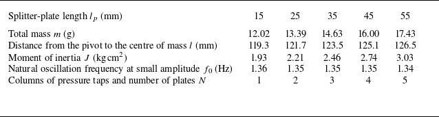

 Cϕ0
 (a)
 CϕQS
 (b)
 β
 lp/d

 lp/d=0.78
 (a)
 Cϕ0
 β
 (b)
 β
 (c−d)
 ΔCp0
 (c)
 σΔCp
 (d)
 (e)
 (d)
 β
 (b−d)
 β=[0,20,33,50]∘
 (a)

 ux¯/U∞
 ux¯/U∞=0
 (a)
 lp/d=0.78
 β
 (b)
 lp/d
 βX
 Cϕ0
 CϕQS

 lp/d=0.78
 Ur=20
 a−c
 d−f
 (a,d)
 ϕ
 (b,e)
 |Wϕ|
 ϕ
 (a,d)
 |Wϕ|
 (c,f)
 β
 ϕ
 (a,d)

 ϕsat
 (a)
 βsat
 (b)
 f/f0
 (c)
 lp/d
 Ur
 ϕsat
 f/f0
 (d)
 (a)

 lp/d=0.78
 Ur=20
 a−b
 c−d
 (a,c)
 ϕ¨
 (b,d)
 ϕ¨aero

 E
 lp/d=0.78
 Ur
 maxT(EK)
 maxT(EP)

 (a)
 Paero
 β
 lp/d=0.78
 (b)
 βsat
 Ur
 lp/d
 βsat
 βX
 (c)
 ϕsat
 βX

 lp/d=0.78
 Ur=20
 a−d
 e−h
 (a,e)
 β
 (b,f)
 (a,e)
 Cϕ3
 (c,g)
 Cϕ3
 (d,h)
 Cϕ3QS

 lp/d=0.78
 Ur=52
 (a)
 β
 (b)
 Cϕi
 Cϕi~
 (c)
 Cϕi

 lp/d=0.78
 Ur=20
 Cϕ~
 β

 Cϕ~
 β
 lp/d=0.78
 Ur=20

 lp/d=0.78
 Ur=20
 (a)
 b−i
 Cϕ~
 β
 (b−i)
 ΔCp~

 lp/d=0.78
 Ur=20
 (a)
 b−i
 Cϕ~
 β
 (b−i)
 ux~/U∞

 CϕQS
 (b)
 lp/d

 βsat
 ϕsat
 (a)
 (b)
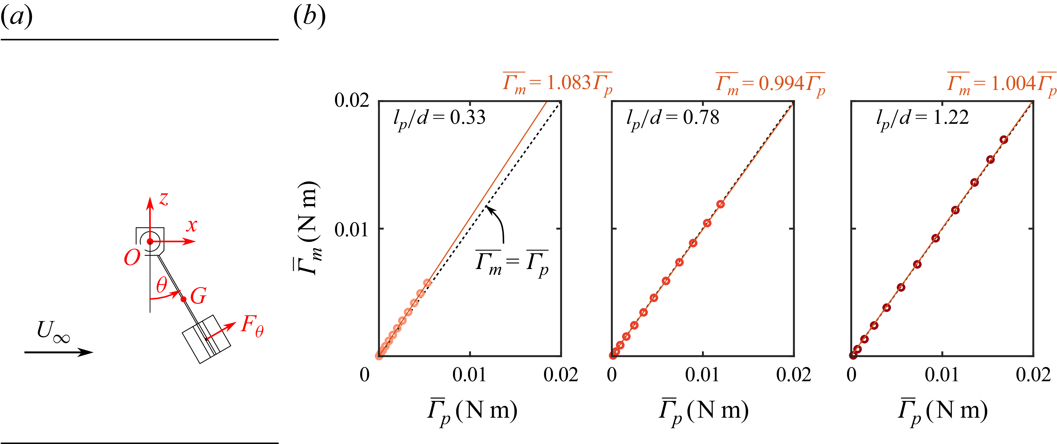
 (a)
 (b)
 Γm
 Γp
 lp/d.

 Open access

