

Introduction
The possibility of graphene-based electronic devices has been and remains a prevalent motivation for graphene research (see the introductory article in this issue). Progress toward this goal, however, continues to be slow because of a narrow, transport-based approach to fundamental graphene research. Although there are many ways of producing graphene, the ability to understand graphene physics is ultimately tied to the interaction of graphene with whatever substrate it is on. With that fact understood, graphene research is advanced only by being able to controllably and reproducibly place graphene on an interface where it can be studied by a wide variety of surface probes. In other words, flat, well-ordered, characterizable samples are required for any substantive progress toward graphene electronics. These conditions exclude graphene produced by exfoliation or chemical vapor deposition (CVD), because methods to transfer graphene to supporting substrates with atomic precision have not yet been developed. Epitaxial graphene (EG), on the other hand, meets all of these requirements and, therefore, is the focus of this review. (See the articles in this issue by Ruan et al., Nyakiti et al., Bartelt and McCarty, Starke et al., and Wong et al. for more information about epitaxial graphene.)
Graphene’s two-dimensional nature necessitates a significant number of surface probes. Because surface probes intrinsically strongly interact with the material, the Born approximation is no longer strictly valid. This makes data from most surface probes difficult to analyze. Therefore, multiple techniques must be employed that measure different aspects of the material structure and electronic properties in order to fully understand the graphene–graphene or graphene–substrate system. The ability to prepare atomically flat graphene films, combined with multiple surface-analysis techniques, allows impurities and substrate effects to be quantified or separated out from different measurements. This process has subsequently contributed to a substantial body of physics information on graphene and graphene devices.
Synchrotron-based surface probes have been at the forefront of graphene research. They include surface x-ray diffraction (SXRD), x-ray and ultraviolet photoemission spectroscopies (XPS and UPS), angle-resolved photoemission spectroscopy (ARPES), photoemission electron microscopy (PEEM), and k-resolved PEEM (k-PEEM). We show not only how these tools have been able to demonstrate many predicted properties of graphene but also, more importantly, how they have allowed significant new discoveries about the electronic structure, some of which are at variance with current models. These new results are inspiring new ideas on how graphene electronics might be realized.
Structure and electronic properties
Graphene’s electronic properties are intimately coupled with its stacking. This relationship is exemplified by graphene grown on the two polar faces of SiC. From the earliest measurements, it was known that graphene grows differently on the (0001) Si face and the (000 $\bar 1$) C face, with Si-face graphene forming an ordered structure, whereas C-face graphene appeared to be rotationally disordered.Reference Van Bommel, Crombeen and Van Tooren1
That early work left a longstanding impression that C-face graphene was too disordered to be useful. The resulting lack of interest led to only two C-face-related articles being published between 1975 and 2003. It was not until a fortuitous accident by a student in the Epitaxial Graphene Lab at Georgia Institute of Technology, who mislabeled a sample, that the incredible mobilities of C-face graphene became apparent.
A comparison of Si-face and C-face graphene
Si-face graphene
Si-face graphene grows commensurate with a SiC (6√3 × 6√3)R30° structure (denoted 6√3 herein), where a 13 × 13 graphene cell is rotated by 30° relative to the SiC substrate as determined by low-energy electron diffraction (LEED) (see Figure 1a).Reference Hass, de Heer and Conrad2 X-ray measurements show that there is an interface layer above the SiC with a low density of silicon atoms thought to be in adatom sites (see Figure 1b). The first structural graphene layer (i.e., a layer with the atomic structure of grapheneReference Rutter, Guisinger, Crain, Jarvis, Stiles, Li, First and Stroscio3) has a relatively short bond distance to this low-density silicon layer.Reference Hass, Millán-Otoya, First and Conrad4 This first structural graphene layer is called the “buffer” layer and does not have the band structure of graphene.
(a,c) Low-energy electron diffraction (LEED) patterns from (a) Si-face and (c) C-face graphene. Subscript G refers to graphene coordinates; coordinates without subscripts correspond to SiC. (b,d) Schematic models of graphene on the (b) Si face and (d) C face of SiC, each with two structural graphene layers. Shaded circles represent carbon atoms; white circles, silicon atoms; and lined circles, graphene carbon atoms.

The very first measurements of graphene’s band structure were carried out using ARPES on Si-face graphene grown in ultrahigh vacuum (UHV).Reference Ohta, Bostwick, McChesney, Seller, Horn and Rotenberg5–Reference Ohta, Bostwick, Seyller, Horn and Rotenberg7 Because this early work was done using UHV-grown graphene, some results were ambiguous because of poor film quality. It was not until 2006, when the first furnace growth techniques were developed, that highly ordered films became availableReference Hass, Feng, Li, Li, Song, de Heer, First, Conrad, Jeffrey and Berger8, Reference Emtsev, Bostwick, Horn, Jobst, Kellogg, Ley, McChesney, Ohta, Reshanov, Röhrl, Rotenberg, Schmid, Waldmann, Weber and Seyller9 (see the later section “Epitaxial graphene growth”).
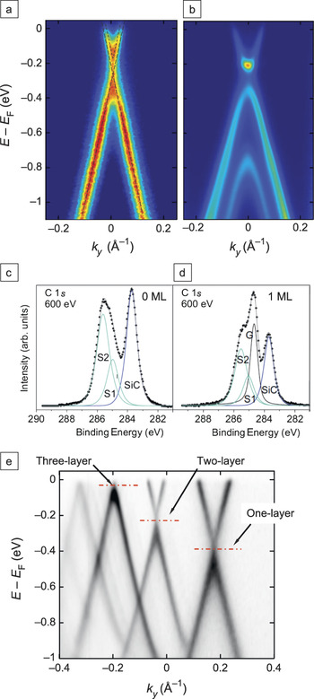
Nonetheless, this early work with UHV-grown films showed three important features of Si-face graphene. First, the graphene is doped by the substrate, as evidenced by a shift below the Fermi energy (E F) of the Dirac energy (E D) where the bands meet (see Figure 2a). For single layers, there is a large n doping: ∼0.44 eV (∼3 × 1013 cm−2). The doping decreases for thicker films.Reference Ohta, Bostwick, McChesney, Seller, Horn and Rotenberg5 The second observation is a distortion in the linear bands near E D. For monolayer films, the upper and lower linear bands appear shifted. This is due to many-body effects (see the later section “Beyond the simple linear bands”).Reference Bostwick, Ohta, Seyller, Horn and Rotenberg12 Finally, Si-face graphene has Bernal (or AB) stacking as in graphite (although later high-resolution tunneling electron microscopy work showed that trilayers can be rhombohedrally stacked as wellReference Norimatsu and Kusunoki13). The Bernal stacking lifts the single-sheet degeneracy and causes a band splitting of ∼0.44 eV plus the formation of a small ∼0.1 eV gap (see Figure 2b).
Angle-resolved photoemission spectroscopy (ARPES) spectra of (a) monolayer and (b) bilayer graphene films above the buffer layer on Si-face SiC, showing the energy E of occupied states below the Fermi level E F as a function of wave vector ky (where ky is perpendicular to the Γ–K direction). The dashed lines in (a) show that the linear bands above and below the Dirac point where the bands meet do not match, whereas the bilayer data in (b) show a small energy gap. (c–d) Carbon 1s spectra from a Si-face graphene (c) buffer layer and (d) monolayer above the buffer layer. S1 and S2 represent surface peaks, and G and SiC have energy shifts corresponding to graphene and silicon carbide, respectively. Reproduced with permission from Reference Reference Riedl, Coletti and Starke10. ©2010, Institute of Physics Publishing. (e) Overlay of a number of ARPES spectra from one-, two-, and three-layer C-face graphene films showing decreasing doping levels. Reproduced with permission from Reference Reference Hicks, Shepperd, Wang and Conrad11. ©2012, Institute of Physics Publishing.

The existence of a Si-face buffer layer is one of the most important early discoveries about EG. Early calculations predicted that the first graphene layer would be insulating.Reference Varchon, Feng, Hass, Li, Ngoc Nguyen, Naud, Mallet, Veuillen, Berger, Conrad and Magaud14 Using ARPES, Emtsev et al.Reference Emtsev, Speck, Seyller, Ley and Riley15 showed that the first graphene layer was electronically not graphene and, in fact, had a gap.Reference Riedl, Zakharov and Starke16Figure 2c–d show carbon 1s spectra from a buffer layer and a monolayer graphene film above the buffer layer, respectively. The buffer-layer film exhibits two surface states plus a SiC-shifted carbon 1s peak. Once the first active graphene layer forms, a graphene-shifted carbon 1s peak appears. The most convincing evidence for an electronically distinct buffer layer was demonstrated by Riedl et al.,Reference Riedl, Coletti, Iwasaki, Zakharov and Starke17 who showed that, upon hydrogenation of the interfacial SiC dangling bonds (see the later section “Controlling the graphene–SiC interface”), the gap at the K point (the corner of the hexagonal Brillouin zone) was replaced by the expected Dirac cone of an isolated graphene layer.
C-face graphene
For growth on C-face SiC, x-ray measurements show that the first structural graphene layer sits above an interface layer that is more carbon-rich than the interface layer on the Si face (the density is close to that of diamond).Reference Hass, Feng, Millàn-Otoya, Li, Sprinkle, First, Berger, de Heer and Conrad18 There are two reconstructions before graphitization: (3 × 3) and (2 × 2).Reference Bernhardt, Nerding, Starke and Heinz19 However, once a graphene diffraction pattern appears, the band structure of graphene is fully developed, indicating that no buffer layer exists on the C face.
The band structure of a single-layer C-face graphene film is very similar to that of a single Si-face graphene layer above the buffer layer (compare Figure 2a with Figure 2e). The doping decreases with increasing thickness, as for Si-face graphene, and the doping levels are nearly the same for the two faces.Reference Hicks, Shepperd, Wang and Conrad11 Similarly, a small distortion (not visible in Figure 2e) in the band linearity near the Dirac point is very similar to that observed for Si-face graphene.Reference Siegel, Park, Hwang, Deslippe, Fedorov, Louie and Lanzara20 (See the later section “Beyond the simple linear bands” for more details.)
The graphene–SiC interface is much more complicated for C-face than Si-face graphene. Not only does C-face graphene yield different carbon 1s spectra than Si-face graphene,Reference Emtsev, Speck, Seyller, Ley and Riley15, Reference Starke and Riedl21 but their spatial variation is complex and not understood. The local work function varies substantially over 50 μm.Reference Mathieu, Barrett, Rault, Zhang, de Heer, Berger, Conrad and Renault22 However, the striking difference between C-face and Si-face graphene is the stacking. C-face graphene is not Bernal stacked. Figure 1c shows a LEED pattern from a C-face film. The pattern shows graphene rotated by both 30° (R30°) and 0° ± 7° (R0°) relative to the SiC (1 × 1) pattern. Both x-rays (a bulk probe) and LEED (a surface probe) show similar angular distributions, indicating that planes throughout the entire film have these multiple orientations.Reference Hass, Varchon, Millàn-Otoya, Sprinkle, Sharma, de Heer, Berger, First, Magaud and Conrad23, Reference Sprinkle, Hicks, Tejeda, Taleb-Ibrahimi, Le Fèvre, Bertran, Tinkey, Clark, Soukiassian, Martinotti, Hass and Conrad24
This LEED pattern was erroneously described as turbostratic,Reference Shallcross, Sharma, Kandelaki and Pankratov25 a term originally coined to describe disordered carbon soot in which non-Bernal planes typically ∼10 nm in diameterReference Hutcheon and Blackman26 are randomly distributed in an otherwise AB-stacked film.Reference Franklin27, Reference Cançado, Pimenta, Saito, Jorio, Ladeira, Grüeneis, Souza-Filho, Dresselhaus and Dresselhaus28 For C-face films, in contrast, systematic SXRD studies showed that both the in-plane structure and the vertical stacking in these films are highly ordered.Reference Sprinkle, Hicks, Tejeda, Taleb-Ibrahimi, Le Fèvre, Bertran, Tinkey, Clark, Soukiassian, Martinotti, Hass and Conrad24 Adjacent sheets are rotated by 30° on average, with Bernal-stacked pairs occurring in less than 15% of the film.Reference Sprinkle, Hicks, Tejeda, Taleb-Ibrahimi, Le Fèvre, Bertran, Tinkey, Clark, Soukiassian, Martinotti, Hass and Conrad24 Similarly, ARPES surveys of the top three layers of C-face graphene showed that less than 20% of adjacent sheets are Bernal stacked.Reference Sprinkle, Hicks, Tejeda, Taleb-Ibrahimi, Le Fèvre, Bertran, Tinkey, Clark, Soukiassian, Martinotti, Hass and Conrad24 These measurements show that, in C-face films, AB-stacked planes are the faults in this unusual stacking mode. We refer to this new stacking arrangement of graphene as multilayer epitaxial graphene (MEG). As we show later in this article, this type of stacking preserves the linear band structure of an isolated graphene sheet.
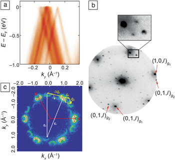
Figure 3a shows a set of linear Dirac cones rotated by different amounts for a MEG film. Two adjacent sheets are called commensurately rotated when the rotated lattice points coincide exactly after a certain number of lattice spacings. The stacked sheets then form a supercell with reciprocal lattice vectors G that depend on the rotation angle.Reference Hass, de Heer and Conrad2, Reference Lopes dos Santos, Peres and Castro Neto30, Reference Mele31 Commensurately rotated graphene has been demonstrated by a number of techniques. Figure 3b shows a microspot LEED image with the rotated supercell spots from a two-layer graphene film.Reference Wang, Shepperd, Hicks, Nevius, Tinkey, Tejeda, Taleb-Ibrahimi, Bertran, Le Fèvre, Torrance, First, de Heer, Zakharov and Conrad29 Although isolated rotated domains can explain the rotated main diffraction peaks, they cannot explain the supercell spots. An even better example is seen in k-PEEM images of the first Brillouin zone (BZ) of C-face graphene. Figure 3c shows a constant-energy cut through two graphene BZs rotated by 21.9°. That they are commensurately rotated is demonstrated by the third replica set of cones flipped in symmetry. Specifically, the replica set of cones is produced by translating a cone from the first BZ by the reciprocal lattice vector of the second BZ (or vice versa). This coherent scattering can occur only if the two sets are commensurately rotated.
(a) ARPES-measured band structure from the top three layers of a 10-layer C-face graphene film near the K point of the Brillouin zone (BZ). ky is perpendicular to the Γ−K direction. Part (a) reproduced with permission from Reference Reference Sprinkle, Hicks, Tejeda, Taleb-Ibrahimi, Le Fèvre, Bertran, Tinkey, Clark, Soukiassian, Martinotti, Hass and Conrad24. ©2010, Institute of Physics Publishing. (b) Microspot LEED image from a two-layer C-face graphene film, where g 1 and g 2 are the reciprocal lattice vectors of the two rotated graphene planes. The inset shows the rotated supercell pattern. Part (b) reproduced with permission from Reference Reference Wang, Shepperd, Hicks, Nevius, Tinkey, Tejeda, Taleb-Ibrahimi, Bertran, Le Fèvre, Torrance, First, de Heer, Zakharov and Conrad29. ©2012, American Physical Society. (c) k-resolved photoemission electron microscopy image of the BZ of a three-layer graphene film at a binding energy of 1.3 eV. The replica Dirac cones are shown shifted by the G vectors of the commensurate supercell. Part (c) reproduced with permission from Reference Reference Mathieu, Barrett, Rault, Zhang, de Heer, Berger, Conrad and Renault22. ©2011, American Physical Society.

Beyond the simple linear bands
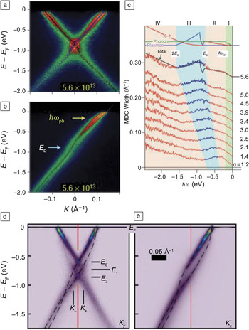
ARPES measurements have shown that the linear bands calculated with a tight-binding (TB) model break down in the presence of high doping levels.Reference Bostwick, Ohta, Seyller, Horn and Rotenberg12, Reference Bostwick, Speck, Seyller, Horn, Polini, Asgari, MacDonald and Rotenberg32 Many-body effects including electron–plasmon and electron–phonon coupling alter the band linearity near the Dirac point for both Si-face and C-face graphene.Reference Bostwick, Ohta, Seyller, Horn and Rotenberg12, Reference Siegel, Park, Hwang, Deslippe, Fedorov, Louie and Lanzara20 As discussed earlier, a distortion is present near the Dirac point in Si-face graphene.Reference Zhou, Gweon, Fedorov, First, de Heer, Lee, Guinea, Castro Neto and Lanzara6, Reference Bostwick, Ohta, Seyller, Horn and Rotenberg12 Although this distortion was originally thought to be due to a substrate-induced gap, it is now known to be caused by many-body effects. Figure 2a shows the Dirac cone from a Si-face one-layer graphene film. The cone is electron doped to E F ≈ E D + 0.38 eV by charge transfer from the substrate. It is clear that the linear bands below E D do not extrapolate to the linear bands above E D. Bostwick et al.Reference Bostwick, Ohta, Seyller, Horn and Rotenberg12 showed that increasing the electron doping using potassium causes the distortion to become larger, as shown in Figure 4a–b.
(a–b) ARPES scans from a potassium-doped, one-monolayer, Si-face graphene film (with an electron doping level of n = 5.6 × 1013 cm−2), showing cuts through the Dirac cone (a) perpendicular to and (b) along the Γ−K direction. The arrows mark two kinks in the linear bands, at the Dirac point E D and below E F by the phonon energy ħωph. (c) Momentum distribution curves (MDCs) of the Dirac cone for different n-doping levels as a function of binding energy, ħω. The doping level (n) is in units of 1013 cm−2. Successive traces are shifted upward by 0.025 Å−1. The simulated total scattering rate (black line) and contributions due to decay into phonons (green), electron–hole (e–h) pairs (red), and plasmons (blue) are compared with the MDC spectral width for the sample with the highest doping level (see Reference Reference Bostwick, Ohta, Seyller, Horn and Rotenberg12). (d–e) Experimental spectral functions of doped graphene with a hydrogen-passivated interface to Si-face SiC (d) perpendicular and (e) parallel to the Γ−K direction. Dashed lines are guides showing the observed hole and plasmaron bands. Red lines mark the K point of the graphene BZ. Reproduced with permission from Reference Reference Bostwick, Speck, Seyller, Horn, Polini, Asgari, MacDonald and Rotenberg32. ©2010, American Association for the Advancement of Science.

The distortion is a direct result of the unusual linear dispersion near the Dirac point in graphene, which increases the number of ways a photoelectron–hole excitation can decay relative to standard Fermi-liquid theory.Reference Bostwick, Ohta, Seyller, Horn and Rotenberg12 For holes just above E D, there are many possible electron–hole creation events that cause the hole to decay to the ground state, enhancing the photon scattering rate and, thus, the photoemission cross section. Holes created just below E D have fewer electron–hole creation possibilities because of insufficient momentum transfer, thus lowering the cross section. This leads to the kink observed at E D in the momentum distribution curves (MDCs) of Figure 4c.
An analysis of the k widths of the MDCs (proportional to the electron scattering rate) for different doping levels shows four energy regions (see Figure 4c). These regions are defined by the thresholds for de-excitation of photoelectrons by the production of phonons, electron–hole pairs, and plasmons. Fits to the MDCs give a coupling constant of λ ≈ 0.3, five times larger than predicted.Reference Calandra and Mauri33 The peak in the scattering rate in Figure 4c at E D is due to plasmon emission. Normally, electron–plasmon coupling is forbidden in two-dimensional and three-dimensional electron gases.Reference Jensen, Bartynski, Gustafsson and Plummer34 The plasmon creation in graphene occurs at ∼1 eV, representing a unique instance where electron–plasmon coupling is kinematically allowed for a purely two-dimensional system.
A difficult-to-observe many-body example is plasmaron bands. Plasmarons are a collective excitation formed by the interaction of charges with plasmons.Reference Lundqvist35 Normally, substrate doping on Si-face graphene leads to high screening that causes the plasmaron band to be barely resolvable. Hydrogen passivation of the SiC–graphene bonds (see the later section “Controlling the graphene–SiC interface”) significantly reduces the graphene–substrate interaction, allowing subtle many-body effects to be measured.Reference Bostwick, Speck, Seyller, Horn, Polini, Asgari, MacDonald and Rotenberg32Figure 4d–e show clearly resolved additional bands in the Dirac cone associated with plasmaron bands. Detailed doping-dependence experiments showed that the spectral function from these bands scale with E F – E D and the Fermi momentum, k F, a key prediction of the one-particle Green’s function random-phase approximation (G0W-RPA) theory.Reference Hwang and Das Sarma36, Reference Polini, Asgari, Borghi, Barlas, Pereg-Barnea and MacDonald37 These works showed that differences between the measured band crossings and the crossing predicted by G0W-RPA differ in detail, suggesting new physics beyond this model.
Comparing theory and experiment
Between 2004 and 2009, graphene theory articles were published at a rate of 7:1 compared to experimental works, so it is worth considering how their predictions stand up to experimental tests. Two research areas, each active both theoretically and experimentally, are particularly relevant to graphene electronics: interlayer interactions and the production of energy gaps in narrow graphene ribbons.
Interlayer interactions
Commensurately rotated graphene provides a unique system for investigating interlayer graphene coupling. Lopes dos Santos et al.Reference Lopes dos Santos, Peres and Castro Neto30 developed an analytic solution to the TB model for small relative rotations using a continuum approximation to treat the interlayer coupling as spatially uniform. This model predicts two observables: First, the two rotated cones, separated by ∆K θ in the BZ (see Figure 5a), rehybridize to form a distorted single cone with a van Hove singularity (VHS; saddle point) halfway between the K and K θ points, as shown in Figure 5c. The second prediction is that the Fermi velocity slows to a renormalized value,  $\tilde v_{\rm{F}} $ (see Figure 5b), that goes to zero as the rotation angle goes to zero (see Figure 6b).Reference Lopes dos Santos, Peres and Castro Neto30 Full TB and ab initio calculations confirmed the continuum-approximation prediction that the renormalized velocity goes to zero very rapidly at rotation angles less than 4°.Reference Trambly de Laissardière, Mayou and Magaud39 The existence of a VHS and a renormalized Fermi velocity was tested by directly measuring the band structure of MEG films. To characterize small relative layer rotations using ARPES, Hicks et al.Reference Hicks, Sprinkle, Shepperd, Wang, Tejeda, Taleb-Ibrahimi, Bertran, Le Fèvre, de Heer, Berger and Conrad38 exploited Umklapp scattering that involves reciprocal lattice vectors of the commensurate supercells in different BZs. Figure 6a shows an example of a Dirac cone from two small-angle commensurately rotated graphene sheets. In contrast to theory, these experiments found no velocity renormalization or VHS within the ∼50 meV experimental resolution. The plot of the measured ARPES velocities in Figure 6b also shows no significant velocity changes even for the smallest measured rotation angles, for which the predicted velocity is an order of magnitude smaller. The lack of a VHS is demonstrated in Figure 6a. The expected TB dispersion is drawn in the figure as a gold dashed line for clarity. Instead of the VHS, the cones cross as straight lines with no discernible singularity.
(a) Schematic Dirac cones of two commensurately rotated graphene sheets, shifted by a vector K θ. (b) Velocity renormalization causes the Fermi velocity, v F, to be smaller than the value for an isolated sheet, making the slopes of the cones smaller in an energy window of  $\Delta E_{\tilde K} $ near the Dirac point. (c) Cut through two rotated Dirac cones with a predicted van Hove singularity formed between the K and K θpoints. Reproduced with permission from Reference Reference Hicks, Sprinkle, Shepperd, Wang, Tejeda, Taleb-Ibrahimi, Bertran, Le Fèvre, de Heer, Berger and Conrad38. ©2011, American Physical Society.

(a) Experimental Dirac cones from a 1.7°-rotated graphene pair show no evidence of mixing. The gold dashed line is the predicted band structure with a van Hove singularity from a continuum tight-binding (TB) model.Reference Franklin27 (b) Comparison of the measured Fermi velocity (circles) with the calculated renormalized Fermi velocity,  $\tilde v_{\rm{F}} $, as a function of rotation angle. The solid line represents a continuum TB calculation of
 $\tilde v_{\rm{F}} $,Reference Franklin27 and the triangles correspond to the low-angle-corrected
 $\tilde v_{\rm{F}} $ values from a full TB calculation;Reference Polini, Asgari, Borghi, Barlas, Pereg-Barnea and MacDonald37 both are expressed relative to the value in a single graphene sheet, v Fo. The experimental values are normalized to the measured average velocity (dashed line) and show no indication of the predicted drop at small angles.

In a potential resolution of this conflict, new theoretical work has shown that the hopping integrals between unaligned sublattices in the two layers (i.e., the non-AB and -AA terms) are vital for an understanding of the two-layer Dirac cone spectrum. Mele showed that these terms lead to a crossing of the cones with no VHS.Reference Mele40 The precise band structure predicted in these calculations has yet to be verified, but ARPES will certainly be crucial to answering this important problem in interlayer interactions.
Gaps
A gap in graphene’s Dirac cones has been predicted to form at the K point as a consequence of either an ordered periodic potentialReference Duplock, Scheffler and Lindan41, Reference Pedersen, Flindt, Pedersen, Mortensen, Jauho and Pedersen42 or finite-size effects.Reference Wakabayashi, Fujita, Ajiki and Sigrist43–Reference Brey and Fertig46 There are a few examples of ordered adsorbate– or substrate–graphene potentials leading to a gap. Transport measurements also suggested that producing thin graphene ribbons can open a gap, but that work is now being questioned.Reference Han, Brant and Kim47, Reference Han, Özyilmaz, Zhang and Kim48 In this section, we present what is known about the state of these predictions as revealed by synchrotron studies.
Gaps from ordered potentials
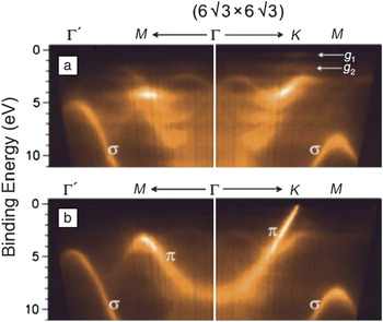
The two best examples of an ordered-potential-induced gap are Si-face bilayer graphene and its buffer layer. As mentioned previously, the Si-face buffer layer is structurally graphene but has no Dirac cone. Figure 7 compares the band structure, measured with ARPES, of the Si-face 6√3 buffer layer alone with that of a graphene ML on top of it. Although there is an envelope characteristic of the linear dispersing π band up to the K point in the buffer layer, it terminates about 2 eV below E F. Two nondispersing localized states, g 1 and g 2, appear in the gap region.Reference Emtsev, Speck, Seyller, Ley and Riley15 These states and the band structure itself are thought to be due to an ordered rehybridized graphene pz orbital bonding with the SiC interface layer. It is important to note that the bonding to SiC is highly ordered. This is demonstrated by the ordered LEED pattern in Figure 1a.
Band maps of SiC(0001) with (a) a (6√3 × 6√3)R30° buffer layer and (b) one monolayer of graphene on top of this buffer layer as obtained by ARPES. The band dispersion of the buffer layer between Γ and K in (a) shows a series of gaps in a band that becomes the π bands in (b). The linearly dispersing π band in the monolayer (b) is replaced in the buffer layer (a) by a distribution of states that disappears close to the Fermi energy to be replaced by two localized states denoted, g 1 and g 2, that exist in the region close to the Fermi energy E Fas indicated in (a). Reproduced with permission from Reference Reference Emtsev, Speck, Seyller, Ley and Riley15. ©2008, American Physical Society.

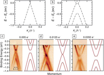
An excellent example of bond ordering inducing a gap is when two graphene sheets are Bernal stacked so that the bonding of the two atoms in the unit cell is nonequivalent. This lifts the degeneracy in the π bands, and two energy-shifted bands appear (compare Figure 8a–b; note that the upper split band is out of the figure range).Reference Riedl, Coletti, Iwasaki, Zakharov and Starke17 Doping at the graphene–SiC interface generates a surface electric field that produces an asymmetric potential in the two layers. The asymmetry contributes to the gap size at the crossing of the π and π* bands, as shown in Figure 8c. Ohta et al.Reference Ohta, Bostwick, Seyller, Horn and Rotenberg7 used n doping to alter the field and thus close and then reopen the gap as demonstrated in Figure 8c–e.
(a–b) Schematics of the band structures of (a) single-layer graphene and (b) an AB-stacked graphene bilayer. (c–e) Closing and reopening of the gap in bilayer graphene gap as a function of potassium doping from experiment (left) and theory (right). The number of electrons per unit cell is indicated at the top of each panel. Parts (c)–(e) reproduced with permission from Reference Reference Ohta, Bostwick, Seyller, Horn and Rotenberg7. ©2006, American Association for the Advancement of Science.

Attempts to open a gap using ordered adsorbates have so far met with mixed success. Nitrophenyl groups were covalently bonded to epitaxial graphene to open a ∼0.4-eV gap.Reference Niyogi, Bekyarova, Itkis, Zhang, Shepperd, Hicks, Sprinkle, Berger, Lau, de Heer, Conrad and Haddon49 Although that work demonstrated that covalently decorating graphene can produce a gap, it has been difficult to order the surface-bound molecules. The bonding disorder leads to a significant broadening of the π bands after chemical modification.
A better example was demonstrated by adsorbing atomic hydrogen on graphene grown by CVD on Ir(111).Reference Balog, Jörgensen, Nilsson, Andersen, Rienks, Bianchi, Fanetti, Lægsgaard, Baraldi, Lizzit, Sljivancanin, Besenbacher, Hammer, Pedersen, Hofmann and Hornekær50 This opened a gap of 0.45 eV at the K point. The success of these experiments was due to a periodic distortion of the graphene lattice caused by an interaction with the underlying iridium surface. The moiré pattern caused by this interaction created preferred absorption sites that built a very high degree of long-range order in the hydrogen adsorbate.
Gaps from finite sizes
It was predicted early on that graphene, when patterned into thin strips (“nanoribbons”), would have a bandgap.Reference Wakabayashi, Fujita, Ajiki and Sigrist43–Reference Brey and Fertig46 Early transport measurements on nanoribbons supported this claim, finding a significant decrease in ribbon conductivity at low gate fields in field-effect devices.Reference Han, Özyilmaz, Zhang and Kim48, Reference Li, Wang, Zhang, Lee and Dai51
However, it soon became apparent that edge roughness has a significant impact on carrier mobilities in nanoribbons less than 50 nm in width.Reference Yang and Murali52 Gaps that were seen in earlier ribbon transport measurements were either smaller or nonexistent in later, similar studies on “unzipped” carbon nanotubes whose edges were known to be smoother.Reference Jiao, Zhang, Wang, Diankov and Dai53, Reference Jiao, Wang, Diankov, Wang and Dai54 As a result, apparent bandgaps that were initially interpretated as arising from finite sizes were reinterpreted as originating from series of quantum dots with mismatched energy levels.Reference Han, Brant and Kim47 Evidence of whether very thin nanoribbons can have a bandgap still remains elusive.
Theoretically, the bandgap size in graphene nanoribbons depends on the exact structure of the edges. Zigzag-edged nanoribbons have a metallic nature, whereas armchair ribbons have a bandgap, E gap, whose size is expected to be inversely proportional to the ribbon width (with a coefficient up to 1 eV nm).Reference Son, Cohen and Louie45, Reference Brey and Fertig46 In light of these predictions, the search for a bandgap using ARPES should involve ribbons narrower than 20 nm so that E gap> 50 meV. Because of these small dimensions, it has not yet been possible to employ photon or electron spectroscopies to study individual nanoribbons. Although high-spatial-resolution ARPES (nano-focused ARPES) will soon come online, progress is being made using conventional ARPES with ordered epitaxial graphene ribbon arrays to measure an average band structure.Reference Hicks, Shepperd, Wang and Conrad11, Reference de Heer, Berger, Ruan, Sprinkle, Li, Hu, Zhang, Hankinson and Conrad55
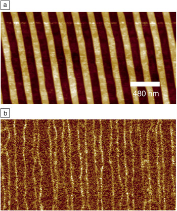
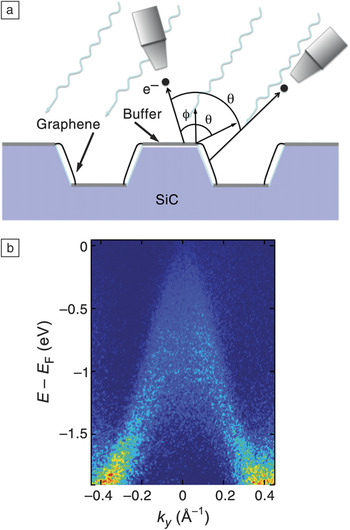
Initially, lithographically patterned EG nanoribbon arrays (with 20-nm widths) were studied, but their ARPES-derived band structure was indistinguishable from that of a continuous EG sheet. Lithography limits prohibited making narrower ribbons, so an alternate approach was developed. By taking advantage of the disparate graphene growth rates on the (0001) and (10 $\bar 1$n) faces of SiC, thin ribbons could be grown on the sidewalls of vertical trenches before the tops became graphitized.Reference Sprinkle, Ruan, Hu, Hankinson, Rubio-Roy, Zhang, Wu, Berger and de Heer56 Dense arrays of sub-20-nm-wide sidewall graphene nanoribbons could be grown, as shown in Figure 9.Reference Hicks, Shepperd, Wang and Conrad11Figure 10a shows a schematic of the experimental geometry for ARPES from postgraphitized faceted trenches. The facet angle is θ ≈ 29°. Figure 10b is an ARPES-derived Dirac cone from a sidewall array with ∼20-nm-wide armchair ribbons. Although the 40-μm ARPES beam sampled ∼160 different ribbons, a Dirac cone is clearly visible. The intensity in this figure is solely from the graphene on the sidewalls because its band structure is physically rotated by θ ≈ ±29° from that of any graphene on the (0001) surface (see Figure 10a).
(a) Atomic force microscopy (AFM) image of a 15-nm-deep trench array in Si-face graphene before graphitization. (b) Electrostatic force microscopy image of the array in (a) after graphitization. Light lines in (b) are the conducting sidewall graphene ribbons.

(a) Schematic of graphene grown on sidewall-faceted Si-face SiC. A detector tilt angle of ϕ is required to observe the K point of the (0001) face. The detector must be rotated by angle θ to observe the sidewall-facet K point. (b) ARPES results from an array of 20-nm-wide sidewall nanoribbons with nominal armchair edges. ky is parallel to the ribbon edge.

Although ARPES appears to corroborate the absence of a bandgap, the apparent lack of a gap in Figure 10b is still not conclusive. It must be remembered that the ARPES spectrum is a spatial average. The facet normal has an angular distribution along the ribbon length because of step-edge disorder. Therefore, the ARPES image is a complicated sum of different sections of the same Dirac cone. New ribbon production methods will soon be available to produce straighter ribbons with significantly smaller widths. The question of whether a gap can form should thus be answered soon.
Controlling the graphene–SiC interface
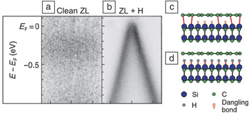
One of the key issues in EG is controlling the graphene–SiC interface. This includes controlling or neutralizing the charge transfer from the SiC to the graphene and electronically decoupling the graphene from the SiC. One of the most important examples of interface control is hydrogen passivation. As discussed in the earlier section “Si-face graphene,” the buffer graphene layer on the Si face is tightly bound to the SiC. Riedl et al.Reference Riedl, Coletti, Iwasaki, Zakharov and Starke17 showed that annealing the buffer layer in H2 at 600°C breaks the sp 3 bonding between the SiC and the buffer layer and removes the two surface peaks in Figure 2c (also see the article in this issue by Starke et al.). This is demonstrated in Figure 11a–b, where the as-grown Si-face buffer layer has no Dirac cone until H2 dosing breaks the bonds to the SiC (see the schematic in Figure 11c–d). There is also a corresponding increase in the mobility of Si-face films after hydrogen absorption.Reference Speck, Ostler, Röhrl, Jobst, Waldmann, Hundhausen, Ley, Weber and Seyller57
(a–b) Band structures determined by ARPES of a Si-face buffer layer (also referred to as the “zero layer,” ZL) measured at the graphene K point: (a) clean surface, for which no bands are visible, and (b) the surface after being heated and exposed to H2, for which the graphene Dirac cone is clearly visible. (c–d) Models of how hydrogen saturates the dangling bonds of the substrate silicon. Reproduced with permission from Reference Reference Riedl, Coletti, Iwasaki, Zakharov and Starke17. ©2009, American Physical Society.

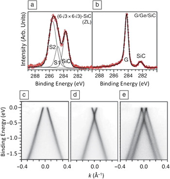
Aside from hydrogen, two other materials are now known to intercalate between graphene and SiC. Using both XPS and LEED, Aït-Mansour et al.Reference Kubler, Aït-Mansour, Diani, Dentel, Bischoff and Derivaz58, Reference Aït-Mansour, Dentel, Kubler, Diani, Derivaz and Bischoff59 showed that germanium deposited on Si-face graphene diffuses to the SiC interface, where it forms a two-dimensional film at temperatures of 700–1300°C. Recent work revealed more details about this germanium intercalation.Reference Emtsev, Zakharov, Coletti, Forti and Starke60Figure 12a–b show the carbon 1s XPS spectra from a Si-face buffer layer film before and after germanium intercalation, respectively. As for the hydrogenated buffer layer, the surface peaks associated with graphene–SiC bonds are gone after germanium intercalation. Two different germanium phases form, depending on the annealing temperature. When the germanium is annealed at 720°C, the graphene is p-doped (Figure 12c), whereas annealing at 920°C causes the graphene to be n-doped (Figure 12d). A mixed phase containing both dopings is also observed at 820°C (Figure 12e).
Carbon 1s x-ray photoemission spectra from a Si-face buffer layer (ZL) (a) before and (b) after germanium intercalation. Three ARPES-measured Dirac cones from intercalated germanium: (c) p-doped phase, (d) n-doped phase, and (c) mixed n- and p-doped phase. Reproduced with permission from Reference Reference Emtsev, Zakharov, Coletti, Forti and Starke60. ©2011, American Physical Society.

Silicon has also been intercalated into both C-face and Si-face graphene–SiC interfaces.Reference Wang, Shepperd, Hicks, Nevius, Tinkey, Tejeda, Taleb-Ibrahimi, Bertran, Le Fèvre, Torrance, First, de Heer, Zakharov and Conrad29, Reference Xia, Watcharinyanon, Zakharov, Yakimova, Hultman, Johansson and Virojanadara61 On the Si face, XPS reveals that the graphene begins to intercalate above ∼800°C.Reference Xia, Watcharinyanon, Zakharov, Yakimova, Hultman, Johansson and Virojanadara61 At 1000°C, the silicon moves back out to the surface, where it can desorb. Unlike for hydrogenated or germanium-intercalated Si-face graphene, there is no significant change in the graphene doping when the silicon moves to the interface.
On C-face graphene, silicon intercalation gives similar results to Si-face experiments, with some exceptions.Reference Wang, Shepperd, Hicks, Nevius, Tinkey, Tejeda, Taleb-Ibrahimi, Bertran, Le Fèvre, Torrance, First, de Heer, Zakharov and Conrad29 The interaction begins at a lower temperature (∼970°C), but no significant doping has been reported. An estimated two monolayers of silicon have been reported to move into this interface. More studies on both C-face and Si-face graphene are proceeding, spurred on by the possibility of modifying the SiC–graphene interaction, through intercalants, to control graphene doping.
Epitaxial graphene growth
One of the greatest puzzles regarding epitaxial graphene growth on SiC is why graphene grows faster on the C face than on the Si face.Reference Hass, de Heer and Conrad2 At the most basic level, graphene growth is controlled by the sublimation of silicon from SiC that liberates carbon to form graphene. However, diffusion of silicon through graphene on either face must be the same. This logic leaves diffusion through the SiC interface layer as the rate-limiting step, because the interface is the only thing different between the two surfaces. It is still hard to imagine how either interface could be more impermeable to silicon than graphene itself.Reference Miura, Kasai, Dino, Nakanishi and Sugimoto62 Recent experiments now show that the faster C-face growth is, in fact, due to heterogeneous channels in the graphene that are nucleated more readily at the C-face interface.Reference Hicks, Shepperd, Wang and Conrad11
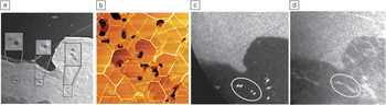
Figure 13a shows a LEEM image from a film with an average of 3 ML of graphene. Dark spots in an 8-ML region are magnified in the insets. These spots are always found in thicker films (more than four layers). Atomic force microscopy images of thick films show similar spots that correspond to very deep depressions in the graphene (see Figure 13b). To show that the spots are tubes running through the graphene, the authors imaged the same area in x-ray photoemission electron microscopy (XPEEM) mode using the SiC-shifted silicon 2p core-level intensity (see Figure 13c). This makes the contrast sensitive to the silicon within the SiC, rather than the unbonded silicon at the surface. The XPEEM map shows the same spots as bright, indicating that the dark spots are holes running from the vacuum to the SiC interface. To demonstrate that the holes are silicon diffusion pathways, silicon was first deposited onto the graphene.Reference Wang, Shepperd, Hicks, Nevius, Tinkey, Tejeda, Taleb-Ibrahimi, Bertran, Le Fèvre, Torrance, First, de Heer, Zakharov and Conrad29 After the sample had been heated, silicon intercalated into the interface (see the section “Controlling the graphene–SiC interface”). An XPEEM image of the same area, this time using the bulk silicon 2p core level for contrast, showed streaking in the vicinity of the holes (see Figure 13d). In other words, there was a higher concentration of silicon near the holes, showing that silicon used these holes as pathways to pass through the graphene and subsequently spread out along the interface.
(a) Low-energy electron microscopy bright-field image (20-μm2) of C-face graphene at –0.05 eV. The insets show silicon “volcanoes” in an eight-monolayer (8-ML) graphene region. (b) AFM image of a 10-μm2 area from 20-ML C-face graphene. (c) X-ray photoemission electron microscopy (XPEEM) image of the same region as in (a) using the SiC-shifted silicon 2p peak for contrast. Dark spots in (a) image here as bright spots, indicating that the dark spots are holes in the graphene. (d) XPEEM image of the bulk silicon 2p peak after intercalation of 6.2 ML of silicon into the graphene–SiC interface. The ellipse defines an area that indicates diffusion of silicon along the interface. Reproduced with permission from Reference Reference Hicks, Shepperd, Wang and Conrad11. ©2012, Institute of Physics Publishing.

One can speculate that the C-face layer promotes excess silicon substitutional sites to nucleate in the graphene. These sites grow in size as more silicon is liberated to form “volcanoes.” For unknown reasons, the nucleation is easier on the C-face interface than on the Si-face interface.
Conclusions
As graphene is a unique system, how this material’s properties can be incorporated into future electronics has yet to be clearly defined. If graphene is to have real potential for advanced electronics, the next step in graphene research must be directed toward understanding how this material interacts with its environment. In particular, graphene electronics research must involve exploring the intimate interaction between graphene and its substrate that alters its properties. Graphene’s properties can change dramatically depending on the substrate it is on. It can behave as a wide-bandgap semiconductor or a metal or exhibit n- or p-type doping simply depending on the support substrate. In the sense that these behaviors cannot yet be predicted, a complete understanding of the graphene–substrate interaction will require significant experimental work. Synchrotron studies have been and will continue to be key to this work.
Much of the recent focus of graphene research has been on growing large films and then exfoliating them onto substrates. Although this is an important research area, determining the potential of graphene for electronics does not depend on meter-size sheets. What is in high demand is a large body of research on how graphene can be manipulated on an insulating or semiconducting substrate to produce desired properties. As for current silicon electronics, highly ordered crystalline heterostructures are key to this work. In this review, we have shown how graphene grown epitaxially on SiC is leading this effort. From an experimental point of view, the atomically controlled epitaxy of graphene has allowed synchrotron-based studies to shed light on the complex relationship of graphene with its support. The future of these efforts is sure to lead to important discoveries and new device architectures for graphene-based electronics.
Acknowledgments
This research was supported by the W.M. Keck Foundation, the Partner University Fund from the Embassy of France, and the NSF under Grants DMR-0820382 (MRSEC) and DMR-1005880. We acknowledge the SOLEIL synchrotron radiation facilities and the Cassiopée beamline. J.H. acknowledges support from the NSF Graduate Research Fellowship Program.