1. Introduction
Being the outer rigid shell of the earth, the lithosphere responds elastically to stress, in contrast to the viscous response of the much softer underlying asthenosphere. The continental lithosphere and the oceanic lithosphere impose very different boundary conditions for the underlying mantle. Being thicker and lighter than the oceanic lithosphere, the continental lithosphere hardly recycles and floats stably above the convective mantle. In contrast, the oceanic lithosphere undergoes a much faster rate of recycling through subduction at oceanic trenches (Hess Reference Hess1962). Analogous to a conveyor belt, the oceanic lithosphere moves away from the mid-oceanic ridges towards oceanic trenches. It thickens as it cools along the way, with a thickness proportional to the square root of its age, just like the thermal boundary layer (TBL) (Turcotte & Schubert Reference Turcotte and Schubert2002). Owing to its fast recycling, the oldest oceanic lithosphere is ∼180 Myr, in contrast to the four billion years age of the oldest continental lithosphere (Condie Reference Condie2005).
Whenever an oceanic lithosphere collides with a continental lithosphere, the former always subducts into the mantle owing to its higher density. Even without collision, when the oceanic lithosphere gets sufficiently old and thick, it becomes unstable and subducts into the mantle, as in the case of the south-west Pacific Ocean trenches. This is analogous to cold plumes triggered by instability falling from the TBL. In this sense, the oceanic lithosphere takes part in mantle convection and constitutes its TBL. The fast recycling rate and the smaller thickness of the oceanic lithosphere (on average half of the continental lithosphere) lead to a much higher average heat flux through it than through the continental lithosphere (Pollack, Hurter & Johnson Reference Pollack, Hurter and Johnson1993; Lenardic Reference Lenardic1998; Grigne & Labrosse Reference Grigne and Labrosse2001; Lenardic et al. Reference Lenardic, Moresi, Jellinek and Manga2005). Consequently, the continental lithosphere acts as a thermal insulator and exerts a thermal blanket effect on the mantle by locally accumulating heat and altering the flow structure, which in turn affects continent motion.
1.1. Laboratory experiments
A prototype laboratory model (Elder Reference Elder1967) was conjured up to capture this thermal–mechanic feedback between a floating continent and the underlying mantle. It is composed of a floating sheet over a thermally convecting fluid heated from below. The floating sheet induced a local thermal anomaly in the underlying fluid, which generates a convective flow that propels the plate. Another simplified model is a floating heat source, either a block or a long line, over a fluid bounded by adiabatic boundaries (Howard, Malkus & Whitehead Reference Howard, Malkus and Whitehead1970; Whitehead Reference Whitehead1972; Mercier et al. Reference Mercier, Ardekani, Allshouse, Doyle and Peacock2014). In these cases, the heat source is propelled by the convective flow it generated and makes periodic excursions between end walls of the fluid container. Remarkably, this periodic oscillation was also observed in a thermally insulating plate drifting over a fluid subject to bottom heating and surface cooling (Zhang & Libchaber Reference Zhang and Libchaber2000; Zhong & Zhang Reference Zhong and Zhang2005, Reference Zhong and Zhang2007).
The above experiments share a common feature in that a local thermal anomaly is introduced into the fluid, through either a heat source or a thermally insulating plate, and this anomaly drives a convective circulation which, in turn, moves the introduced object. This introduction of a thermal anomaly is exactly what a thick floating continent does to the underlying convective mantle and, therefore, continent motion is expected to be influenced by its thermal blanket effect.
Although these experiments shed important light on the thermal blanket effect, none of them added internal heating in the fluid, which is the primary source in the mantle thermal budget (Wasserburg et al. Reference Wasserburg, MacDonald, Holy and Fowler1964). The earth mantle is heated both by the heat flux at the core–mantle boundary (CMB) and the internal heating generated by the radioactive decay. Although the exact proportion of these two heating sources is still controversial, a consensus is that internal heating is the primary source (Davies Reference Davies1988; Sleep Reference Sleep1990; Buffett Reference Buffett2002; Murakami et al. Reference Murakami, Hirose, Kawamura, Sata and Ohishi2004; Oganov & Ono Reference Oganov and Ono2004; van der Hilst et al. Reference van der Hilst, de Hoop, Wang, Shim, Ma and Tenorio2007). How does the addition of internal heating affect the thermal blanket effect of continents?
Convection driven by internal heating has indeed been realised in laboratory experiments through electrolytically heated water (Tritton & Zarraga Reference Tritton and Zarraga1967; Schwiderski & Schwab Reference Schwiderski and Schwab1971) and, more recently, using microwave heating (Fourel et al. Reference Fourel, Limare, Jaupart, Surducan, Farnetani, Kaminski, Neamtu and Surducan2017). The former method encountered the problem of non-uniform internal heating owing to the variation of electrical conductivity with temperature (Schwiderski & Schwab Reference Schwiderski and Schwab1971). Moreover, these experiments include no insulating plate and, therefore, no thermal blanket effect.
1.2. Numerical simulations
The large difference of the Prandtl number of the experimental fluids (∼10 for water and ∼103 for oil) from the value of the Earth mantle (∼1023) brings further uncertainty when relating the results to real Earth cases. Although an Earth-like Prandtl number and a hybrid heating mode may be challenging for laboratory experiments, these conditions are easy to realise in numerical simulations. In fact, the establishment of the theory of plate tectonics stimulates not only laboratory experiments, but also almost concurrent numerical simulations.
1.2.1. Early simulations with no thermal blanket effect
For an infinite-Prandtl-number fluid driven by both bottom and internal heating, simulation results show that the percentage of internal heating strongly affects the flow pattern and boundary-layer stability (McKenzie, Roberts & Weis, Reference McKenzie, Roberts and Weiss1974): as the percentage increases, the width of the up-welling region increases and the top boundary layer becomes more unstable. Compared with pure bottom heating, adding internal heating has also been shown to increase the mean temperature and surface heat flux (Sotin & Labrosse Reference Sotin and Labrosse1999). Nevertheless, these simulations include no plate and thus no thermal blanket effect.
A few studies simulate mantle flow driven solely by plate motion through a prescribed top boundary velocity, with no buoyant force (Davies Reference Davies1977a ,Reference Davies b ; Hager & O’Connell Reference Hager and O’Connell1978, Reference Hager and O’Connell1979), or with buoyant force through either bottom heating (Torrance & Turcotte Reference Torrance and Turcotte1971) or internal heating (Parmentier & Turcotte Reference Parmentier and Turcotte1978; Hager & O’Connell Reference Hager and O’Connell1981; Bunge & Richards Reference Bunge and Richards1996) or both (Davies Reference Davies1986). Among them, some also include a high-viscosity lithosphere (Torrance & Turcotte Reference Torrance and Turcotte1971; Parmentier & Turcotte Reference Parmentier and Turcotte1978; Hager & O’Connell Reference Hager and O’Connell1981) and multiple plates with different piecewise uniform velocities (Hager & O’Connell Reference Hager and O’Connell1981; Davies Reference Davies1986) or velocities from global plate motions (Bunge & Richards Reference Bunge and Richards1996).
These studies using prescribed top boundary velocities favour the ‘top-down’ mechanism which assumes that mantle circulation is driven dominantly by the lithosphere motion. Nevertheless, a primary issue of these simulations is the self-consistency of the coupled dynamic system, in which plate motion should be driven by buoyancy rather than prescribed as a priori. Further, these simulations do not differentiate the thermal boundary condition between continental and oceanic plates, and thus exclude the thermal blanket effect of continents, which is one of the focuses of the present study.
1.2.2. Simulations with the thermal blanket effect but with fixed continents
Numerical simulations that account for the thermal blanket effect have revealed the insulating effect of a newly aggregated supercontinent on mantle flow (Lowman & Jarvis Reference Lowman and Jarvis1993, Reference Lowman and Jarvis1995; Lowman & Gable Reference Lowman and Gable1999; Yoshida, Iwase & Honda Reference Yoshida, Iwase and Honda1999; Honda et al. Reference Honda, Yoshida, Ootorii and Iwase2000; Coltice et al. Reference Coltice, Phillips, Bertrand, Ricard and Rey2007, Reference Coltice, Bertrand, Rey, Jourdan, Phillips and Ricard2009; O’Neill et al. Reference O’Neill, Lenardic, Jellinek and Moresi2009; Heron & Lowman Reference Heron and Lowman2011), including the warming of the mantle, plume generation and flow reversal underneath the supercontinents. A lower percentage of internal heating favours sustained flow reversal underneath the newly aggregated supercontinent (Lowman & Jarvis Reference Lowman and Jarvis1993, Reference Lowman and Jarvis1995). The ratio of internal to basal heating is also important for the style of mantle flow, since hot plumes do not operate in purely internally heated cases (Coltice et al. Reference Coltice, Phillips, Bertrand, Ricard and Rey2007). Further, an enhanced internal heating speeds up plume generation underneath the supercontinent (Yoshida et al. Reference Yoshida, Iwase and Honda1999; Honda et al. Reference Honda, Yoshida, Ootorii and Iwase2000). Almost all these simulations adopt a hybrid heating mode that includes both bottom and internal heating, except one end member case of pure internal heating (Coltice et al. Reference Coltice, Phillips, Bertrand, Ricard and Rey2007).
For purely bottom-heated cases, the effects of continent thickness, width, configuration and thermal properties on mantle heat flow have been revealed through scaling analysis and numerical simulations (Lenardic & Moresi Reference Lenardic and Moresi2001; Grigné, Labrosse & Tackley Reference Grigne, Labrosse and Tackley2007a ,Reference Grigne, Labrosse and Tackley b ; Cooper, Moresi & Lenardic Reference Cooper, Moresi and Lenardic2013).
The periodic boundary or a spherical shell geometry adopted in most of the above simulations allows a relative motion between the continent and the mantle flow. Nevertheless, continent motion is not the focus of these studies. Instead, they focus on the one-way effect of continental thermal insulation on mantle convection. The long-term dynamic interaction between continent motion and the underlying flow structure is not revealed in these studies.
1.2.3. Simulations incorporating both the thermal blanket effect and continent motion
Such a long-term dynamic interaction is revealed in simulations that incorporate a self-consistent continent motion (Gurnis Reference Gurnis1988; Gurnis & Zhong Reference Gurnis and Zhong1991; Zhong & Gurnis Reference Zhong and Gurnis1993; Phillips & Bunge Reference Phillips and Bunge2005; Whitehead & Behn Reference Whitehead and Behn2015; Mao, Zhong & Zhang Reference Mao, Zhong and Zhang2019; Mao Reference Mao2021, Reference Mao2022; Huang Reference Huang2024). Early studies focus more on the dynamic thermal–mechanic feedback (Gurnis Reference Gurnis1988; Gurnis & Zhong Reference Gurnis and Zhong1991; Zhong & Gurnis Reference Zhong and Gurnis1993): a continent moves along with the mantle flow towards a cold down-welling and its encounter with the cold down-welling slows its motion, but its thermal blanket effect gradually weakens the cold down-welling and cultivates a hot up-welling underneath it which, in turn, boosts continent motion. These studies also show that the presence of continents leads to an increased wavelength of convection compared with cases with no continent. Moreover, a more persistent continent motion is observed for larger continents, although the small number of cases in early studies prevents a firm conclusion. This size effect on continent motion is also observed in later three-dimensional spherical simulations (Phillips & Bunge Reference Phillips and Bunge2005). The more recent study of Whitehead & Behn (Reference Whitehead and Behn2015) also draws attention to the size effect on continent motion, showing a unidirectional motion of relatively large continents.
These results stimulate the later systematic investigation on the effect of continent size on both continent motion and flow structure (Mao et al. Reference Mao, Zhong and Zhang2019; Mao Reference Mao2021, Reference Mao2022). As continent size increases, it becomes increasingly capable to alter the impeding flow and continue its motion; this results in an increasingly persistent continent motion, transitioning from long-term stagnancy over cold down-welling to short-term stagnancy over hot up-welling, and eventually to a unidirectionally moving mode (UMM). The critical size for the UMM has been predicted by different simplified models whose parameters are determined from simulation results (Mao Reference Mao2021, Reference Mao2022; Huang Reference Huang2024). Moreover, continent slowdown is observed to be accompanied by a decreased wavelength of convection (Mao Reference Mao2021).
1.3. Motivations for the present study
Apart from the effect of continent size on the dynamic coupling, some of the studies mentioned in § 1.2.3 also offer a glimpse of the effect of internal heating, although far less systematic. This is achieved by comparing results of purely bottom heating with those that add internal heating (Zhong & Gurnis Reference Zhong and Gurnis1993; Whitehead & Behn Reference Whitehead and Behn2015; Mao et al. Reference Mao, Zhong and Zhang2019; Mao Reference Mao2021). A consistent finding is that the addition of internal heating leads to a more persistent continent motion. Further, it also increases the root-mean-square temperature in the top TBL (Zhong & Gurnis Reference Zhong and Gurnis1993) and leads to a more concentrated distribution of continent speed for the UMM (Mao Reference Mao, Zhong and Zhang2019). Nevertheless, the few plate widths (two at most) adopted in previous studies fail to provide a panorama and hamper a thorough understanding of the effect. For example, how does the effect of adding internal heating vary with plate size? Since the addition of internal heating enhances continent mobility, will it decrease the critical plate size for the UMM? Further, will new plate–fluid coupling modes emerge with the addition of internal heating? These questions motivate the present study which adopts a wide range of continent sizes and different intensities of internal heating. Results of numerical simulation answer all the above questions. In particular, the addition of internal heating brings a new coupling mode, i.e. the permanent stagnant mode (PSM), and decreases the critical size for the UMM.
A hybrid heating mode that includes both bottom and internal heating mimics the reality of the Earth better than the end member modes. Following the previous investigations of Mao (Reference Mao2021, Reference Mao2022), which focus on the purely bottom-heating case, the present study adds different intensities of internal heating to the previous cases and focuses on the variation of the thermal blanket effect caused by this addition. Since for the Earth, the internal-heating intensity decays with time (Turcotte & Schubert Reference Turcotte and Schubert2002) and continental scale grows with time (Hart Reference Hart1969), simulations with various internal-heating intensities and plate sizes facilitate an understanding of the evolution of the thermal blanket effect with time.
The remainder of the paper is organised as follows. First, the numerical model and techniques are described in § 2. Section 3 provides an overview of the effect of internal heating intensity on plate motion and coupling mode. Section 4 compares the flow field, plate velocity and coupling mode between purely bottom-heated cases and those that add internal heating. This is followed by a more systematic revelation in § 5 of plate speed and the up- and down-welling location, in which the transition to the UMM and the PSM are shown to occur at a decreased plate size as internal heating intensifies. Section 6 shows the mean flow field for the UMM and the PSM, and compares the length of the ‘propelling’ convection cell with that of other cells. In § 7, a simplified model explains the decreased critical size for the UMM under enhanced internal heating, and an analysis on the top TBL stability explains the emergence of the PSM. Finally, geological implications of the results are discussed in § 8, in particular, the possible effect of a decaying internal heating on continent evolution on Earth and on the migration of the Tharsis volcanism on Mars.
2. Model configuration and numerical methods
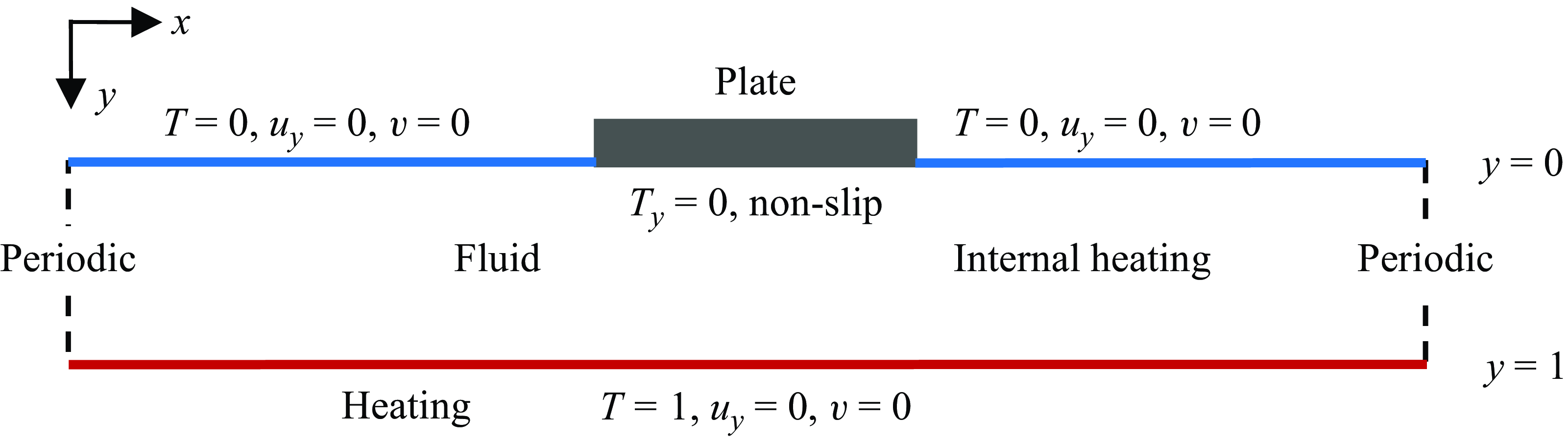
The present model configuration and numerical methods have been described by Mao (Reference Mao2021), except that internal heating is added to the convective fluid. A thermally insulating plate, representing the continent, is introduced to the top of a two-dimensional (2-D) rectangular domain with an aspect ratio of eight (figure 1, A = L/D = 8, where A is the aspect ratio, L and D are the width and depth of the fluid domain). Twelve plate widths are selected over a wide range, from 0.25 to 7 (normalised by the fluid depth). Simplifications used in previous studies (for example, Gurnis Reference Gurnis1988; Whitehead & Behn Reference Whitehead and Behn2015; Mao et al. Reference Mao, Zhong and Zhang2019; Mao Reference Mao2021, Reference Mao2022) are also incorporated here, including the Boussinesq approximation, a uniform fluid viscosity, and the dropping of the inertia and advection terms in the momentum equation owing to the large Prandtl number (∼1023) of the mantle.
Sketch of the model and specification of the boundary conditions.

Here, realistic earth factors such as a spherical geometry, the composition-, temperature- and stress-dependent viscosity, compressibility, and phase changes are excluded to avoid further complexity. A simplified model is advantageous in that it enables the study of a single factor in isolation and thus facilitates quantification for its effect. Instead of attempting to simulate the earth, the present study seeks to find out whether internal heating intensity poses a first-order effect on continent motion and the dynamic coupling mode. The dimensionless governing equations in a Cartesian coordinate system in the indicial notation are
 \begin{equation} \frac{\partial u_{i}}{\partial x_{i}}=0, \end{equation}
 \begin{equation} \frac{\partial ^{2}u_{i}}{\partial x_{j}\partial x_{j}}=Ra\frac{\partial P}{\partial x_{i}}+Ra\delta _{i2}T, \end{equation}
 \begin{equation} \frac{\partial T}{\partial t}+u_{j}\frac{\partial T}{\partial x_{j}}=\frac{\partial ^{2}T}{\partial x_{j}\partial x_{j}}+h, \end{equation}
where the horizontal and vertical coordinates are denoted by x
1 (positive rightward) and x
2 (positive downward), with the corresponding velocity components denoted by u
1 and u
2. These indicial notation are used only in the governing equations (2.1)–(2.3) for simplicity, and are substituted elsewhere by the basic Cartesian notions, i.e. x = x
1, y = x
2, and u = u
1, v = u
2. The symbols t, P, T,
 $\delta$
, h represent time, pressure, temperature (relative to the top boundary), Kronecker delta and internal heating rate respectively, and Ra is the Rayleigh number defined as
 \begin{equation} Ra=\frac{g\beta \Delta TD^{3}}{v\kappa }, \end{equation}
where g,
 $\beta$
,
 $\Delta$
T, v,
 $\kappa$
represent acceleration due to gravity, thermal expansion coefficient, temperature difference between the bottom and the top boundaries, kinematic viscosity, and thermal diffusivity of the fluid, respectively. The scales for the dimensionless variables in (2.1)–(2.3) are D for x
i
,
 $\Delta$
T for T, D
2/
 $\kappa$
for t,
 $\kappa$
/D for u
i
,
 $\rho$
g
 $\beta\Delta$
T for P (
 $\rho$
is fluid density),
 $\rho$
c
p
 $\Delta$
T
 $\kappa$
/D
2 (c
p
is the specific heat) for h. The Rayleigh number Ra is set to be 5 × 10⁷ for all the following simulations, which lies within the range of 107–109 generally attributed to Earth (Turcotte & Schubert Reference Turcotte and Schubert2002; Whitehead & Behn Reference Whitehead and Behn2015).
The Rayleigh number in (2.4) is defined for Rayleigh–Bénard convection subject to pure bottom heating. For purely internally heated convection, another non-dimensional parameter, i.e. the Robert–Rayleigh number, Ra i , is defined based on the internal heating rate H (Roberts Reference Roberts1967; Goluskin Reference Goluskin2015; Goluskin & van der Poel Reference Goluskin and van der Poel2016; Arslan et al. Reference Arslan, Fantuzzi, Craske and Wynn2021, Reference Arslan, Fantuzzi, Graske and Wynn2023; Creyssels Reference Creyssels2021; Wang, Lohse & Shishkina Reference Wang, Lohse and Shishkina2021),
 \begin{equation} Ra_{i}=\frac{g\beta D^{5}H}{v\kappa ^{2}\rho c_{p}}, \end{equation}
where
 ${H}/{(\rho c_{p})}$
represents the temperature source term in the energy equation. Since the dimensional internal heating rate H is normalised by
 $\rho c_{p}\Delta T\kappa /D^{2}$
into a non-dimensional h in the present study,
 $Ra_{i}$
can be expressed with a non-dimensional h as
 \begin{equation} Ra_{i}=\frac{g\beta D^{3}\Delta Th}{v\kappa } = Rah. \end{equation}
For hybrid heating cases with no plate, addition of internal heating has been shown to increase the surface heat flux (Sotin & Labrosse Reference Sotin and Labrosse1999). Therefore, cases with an addition of internal heating are expected to be at a higher degree of vigour or effective Rayleigh number, better represented by Robert–Rayleigh number Ra i than Ra which accounts for only bottom heating. The maximum internal heating rate in the present study is h = 16, resulting in a maximum Ra i of 8 × 10⁸, which also lies within the range (107–109) generally attributed to Earth (Turcotte & Schubert Reference Turcotte and Schubert2002; Whitehead & Behn Reference Whitehead and Behn2015).
The fluid is initially stationery and isothermal (T = 1). A sudden cooling (T = 0) is imposed at the fluid top (y = 0) except at the plate–fluid interface, which is set to be adiabatic (
 $\partial T/\partial y=0$
), a simplified extreme condition to highlight the thermal blanket effect of a continent. Bottom heating of the fluid is embodied by a constant temperature of T = 1 at the bottom (y = 1), and three internal heating rates, h = 0, 8, 16, are selected for all plate widths. The vertical boundaries of the fluid domain are set to be periodic, allowing the fluid and the plate to move out of one side and into the other. The top and bottom boundaries of the fluid are set to be stress-free, except at the plate–fluid interface, which is set to be no slip, i.e. flow velocity at the interface is the same as the plate velocity. For fluid with infinite Prandtl number, there is no acceleration or net force on any mass element since body forces are balanced by viscous forces, and thus the plate has no inertia (Gable, O’Connell & Travis Reference Gable, O’Connell and Travis1991). Similar to previous studies (Mao et al. Reference Mao, Zhong and Zhang2019; Mao Reference Mao2021, Reference Mao2022), plate velocity is determined by the average flow velocity at the first grid cell below the interface. This setting was first used by Gable, O’Connell and Travis (Reference Gable, O’Connell and Travis1991). It ensures a zero net horizontal shear force on the plate–fluid interface, and therefore neither adds nor subtracts energy from the convecting system.
Incorporating the above initial and boundary conditions, the governing equations (2.1)–(2.3) are advanced numerically in time using the finite volume method. The code has been validated when solving natural convection problems (for example, Mao et al. Reference Mao, Lei and Patterson2009, Reference Mao, Lei and Patterson2010). For pressure–velocity coupling, the semi-implicit method for the pressure-linked equations scheme (Patankar Reference Patankar1980) is adopted. The spatial derivatives are approximated through the quadratic upstream interpolation for the convective kinematics scheme (Leonard Reference Leonard1979). A previous study has conducted mesh and time step dependency tests (Mao Reference Mao2021), in which five different meshes were adopted and the error of Nusselt number converges from 44.3 % to 3.8 % as the mesh density increases from 800 × 100 to 2000 × 250. Based on the previous tests (Mao Reference Mao2021) and a trade-off between computation time and accuracy, an equidistant mesh of 2000 × 250 is selected with a time step of 6 × 10⁻⁸.
3. Effect of internal heating intensity on plate motion and coupling mode
3.1. Variation of plate motion with internal heating rate
Plate motion varies significantly with both plate width W and internal heating intensity h (figure 2). For cases with no internal heating (h = 0), small plates move sporadically (figure 2
a) and the average plate speed increases with plate width, peaking somewhere between W = 2.5 and W = 3.0, and decreases with W afterwards (figure 2
d); as plate size increases, plate motion becomes increasingly persistent and less likely to reverse, with a unidirectional motion emerging at a size of somewhere between W = 2.0 and W = 2.5, as suggested by the straight trajectories of large plates (figure 2
a). Although for W
 $ \gt $
3.0, the average plate speed decreases with plate size (figure 2
a,d), the motion remains unidirectional (figure 2
a). However, as internal heating is switched on, an entirely different scenario emerges. Instead of moving unidirectionally, large plates become extremely stagnant, making only small excursions over the entire duration (figures 2
b and 2
c); the average plate speed drops dramatically (figure 2
d) and the undulations of plate trajectories suggest frequent reversal events. All these features suggest an entirely different motion, which will later be revealed to be a PSM, in which the plate oscillates permanently above a hot up-welling.
Variation of plate motion with plate width W and internal heating intensity h. (a–c) Plate trajectories: (a) h = 0; (b) h = 8; (c) h = 16. The inset in panels (b) and (c) zooms in on the stagnant region where only minor displacements occur over the entire duration. For h = 8 and 16, trajectories of large plates fall into this stagnant region. (d) Average plate speed |u
p
| =
 $\langle |\dot{x}_{p}|\rangle$
. For h = 8 and 16, the value of |u
p
| drops abruptly as indicated by the dashed lines, corresponding to the transition of the system to a permanent stagnant mode (PSM). This abrupt drop is absent for h = 0, where no PSM occurs.

A comparison between results of h = 8 and h = 16 suggests this PSM emerges at a decreased plate size as internal heating intensifies, shrinking from W = 4 for h = 8 to W = 3 for h = 16 (figure 2 b–d). Meanwhile, as internal heating intensifies, the mobility of small plates enhances and their motion becomes increasingly persistent, as shown by the decreasing reversal events (figure 2 b,c) and the increasing average speed (figure 2 d). Owing to this enhanced mobility, the unidirectional motion starts to emerge at a decreased plate size, shrinking from W = 2.0 for h = 8 to W = 1.5 for h = 16 (figure 2 b,c). The advent of the unidirectional motion is accompanied by the peaking of the average plate speed (figure 2 d). The peak speed increases with internal heating rate h, whereas the plate size corresponding to the peak decreases with h (figure 2 d).
3.2. Variation of the coupling mode with internal heating rate
Plate motion manifests the flow structure underneath. A coherent flow exerts a coherent force on the plate and moves it towards the same direction, whereas in cases of divergent or convergent flows, the presence of opposing flows results in counteraction of the forces and therefore more stagnant plate motion.
Since the presence of up-wellings or down-wellings is characterised by the sign switch of stream function
 $\Psi$
, the horizontal location of the up-wellings and down-wellings, denoted as x
U
(i) and x
D
(i), where i = 1, … n (n is the number of up- or down-wellings), are identified by where
 $\Psi$
switches sign at the middle depth (y = 0.5).
 \begin{equation} \!\!\!\begin{array}{l} \left\{\begin{array}{l} \!\!x_{U}\left(i\right)\colon\\[6pt]\!\!=\left\{x\left| \ \text{where sign}\left(\Psi \right)\ \text{switches from }-1\text{ to }1\text{ at } y=0.5\ \text{in the positive direction of }x\right.\right\}\!,\\[10pt]\!\!x_{D}\left(i\right)\colon\\[6pt] \!\!=\left\{x\left|\ \text{where sign}\left(\Psi \right)\ \text{switches from }1\text{ to }-1\text{ at }y=0.5\ \text{in the positive direction of }x\right.\right\} \end{array}\right.\\[10pt] \qquad \quad\,\ i=1,2,3\cdots n,\ \text{ where }n\ \text{is the number of up- or down-wellings}, \end{array} \end{equation}
These up- and down-welling positions mark the edge of convection cells at the middle depth. At a particular moment, the convection cell that dominates in propelling the plate is called the dominant cell, or the ‘propelling’ cell. Candidates for the dominant cell should satisfy the following two prerequisites.
-
(i) At least part of it is underneath the plate. In the plate reference frame where the centre of the plate bottom is placed at x = 0 and y = 0, plate edges locate at x =
 $-{W}/{2}$
and
${W}/{2}$
, and thus this condition translates to
$\min (x_{U}(i),\,x_{D}(i))\lt {W}/{2}$
and
$\max (x_{U}(i),\,x_{D}(i))\gt -{W}/{2}$
.
-
(ii) It has a surface flow in the same direction as the plate motion. Therefore, for positive plate speed, i.e. u p
$ \gt $
0, the up-welling of the candidate cell should locate on the left of the down-welling,
$x_{U}(i)\lt x_{D}(i)$
, and vice versa,
$x_{U}(i)\gt x_{D}(i)$
for u
p
$ \lt $
0.


If only one convection cell satisfies these two prerequisites, then it is the dominant cell. In case more than one convection cell satisfies these prerequisites, the dominant cell is the one that contributes most to plate motion. The contribution of each of these candidates of the dominant cell to plate motion is assessed through the stream function. Since stream function
 $\Psi$
at the middle depth y = 0.5 represents an integration of the horizontal flow speed in the upper layer, the strength of surface flow at any x is estimated based on |
 $\Psi$
(x, y = 0.5)|. The dominant cell, denoted as c
d, is the one with the maximum horizontal integration of |
 $\Psi$
(x, y = 0.5)| over its range underneath the plate:
 \begin{equation} c_{d}=\mathrm{arg\ max}\left\{\int _{a\left(C_{k}\right)}^{b\left(C_{k}\right)}\left| \Psi \left(x,y=0.5\right)\right| {\rm d}x,\ k=1,2,\ldots m\right\}, \end{equation}
where m is the number of candidates for the dominant convection cell, C k denotes the kth candidate and [a(C k ), b(C k )] is the horizontal range of cell C k underneath the plate. In the plate reference frame where the centre of plate bottom is at x = 0 and y = 0, the horizontal range [a(C k ), b(C k )] translates into:
 \begin{equation} \begin{array}{l} \left[a\left(C_{k}\right)\!,b\left(C_{k}\right)\right]\\[8pt] =\left\{\begin{array}{l} \left[-\frac{W}{2},\max \left(x_{U}(k),x_{D}(k)\right)\right] \\[8pt] \qquad \text{if min}\left(x_{U}(k),x_{D}(k)\right)\lt -\frac{W}{2}\text{ and max}\left(x_{U}(k),x_{D}(k)\right)\lt \frac{W}{2}\\[8pt] \left[\min \left(x_{U}(k),x_{D}(k)\right)\!,\frac{W}{2}\right] \\[8pt] \qquad \text{if min}\left(x_{U}(k),x_{D}(k)\right)\gt -\frac{W}{2} \text{ and max} \left(x_{U}(k),x_{D}(k)\right)\gt \frac{W}{2}\\[8pt] \left[\min \left(x_{U}(k),x_{D}(k)\right)\!,\max \left(x_{U}(k),x_{D}(k)\right)\right] \\[8pt] \qquad \text{ if min} \left(x_{U}(k),x_{D}(k)\right)\gt -\frac{W}{2}\text{ and max} \left(x_{U}(k),x_{D}(k)\right)\lt \frac{W}{2} \end{array}\right. \end{array} \end{equation}
The case of
 $\min (x_{U}(k),x_{D}(k))\lt -{W}/{2}\text{ and }\max (x_{U}(k),x_{D}(k))\gt {W}/{2}$
is not listed in (3.3) because it is not relevant, since in this case, cell c
k
is the only cell underneath the plate and thus is undoubtly the dominant cell without using (3.2).
(a) Four different instantaneous plate–fluid coupling modes categorised by the presence of up-welling (‘U’) and down-welling (‘D’) underneath the plate: mode ‘D’, down-welling only; mode ‘U’, up-welling only; mode ‘N’, no up-welling or down-welling; mode ‘B, both up-welling and down-welling. (b–d) Percentage of each mode over time for cases of different plate widths W and internal heating rates h: (b) h = 0; (c) h = 8; (d) h = 16. The grey boxes in panels (c) and (d) highlight cases in the permanently stagnant mode (PSM).

In case the number of candidates is larger than one, i.e. m≥ 2, the dominant cell is identified by (3.2). Correspondingly, the dominant up-welling and down-welling are those bounding the dominant convection cell. Let P be the horizontal range of the plate, and the horizontal locations of the dominant up-welling and down-welling, denoted as x u and x d , respectively, categorise the instantaneous flow structure underneath the plate into four modes (figure 3 a).
-
(i) Mode ‘D’, down-welling only, i.e. x u
$\notin$
P and x
d
$\in$
P. This is a stable mode in that any plate motion away from the balanced position will be inhibited by an opposing force and, therefore, the plate is stably trapped, analogous to a ball on a concave surface. The plate will be permanently trapped in this mode if not for the thermal blanket effect, which gradually warms up the underlying flow and eventually alters the flow structure (Mao Reference Mao2022). Since the thermal blanket effect enhances with both plate size and internal heating rate, this mode dominates only the small-plate cases with no internal heating (h = 0, figure 3
b). -
(ii) Mode ‘U’, up-welling only, i.e. x u
$\in$
P and x
d
$\notin$
P. Unlike mode ‘D’, mode ‘U’ is an unstable mode in that any disturbances away from the balanced position will be magnified rather than inhibited, analogous to a ball on a convex surface. This instability endows mode ‘U’ with a transient feature and thus it never dominates the small-plate cases (figure 3). Nevertheless, for large-plate cases with internal heating, mode ‘U’ becomes the only possible mode (figure 3
c,d), which will later be shown to be the PSM. -
(iii) Mode ‘N’, no up-welling or down-welling, i.e. x u
$\notin$
P and x
d
$\notin$
P. This mode is characterised by a coherent flow underneath the plate and therefore signifies high plate speed. Cases with a high percentage of this mode (figure 3
b–d) indeed have high average plate speeds (figure 2
d). -
(iv) Mode ‘B’, both up-welling and down-welling, i.e. x u
$\in$
P and x
d
$\in$
P. This mode is characterised by the coexistence of convergent and divergent flows underneath the plate. It dominates the very large plate cases with no internal heating (figure 3
b). The presence of opposing flows decreases the plate speed for these cases (figure 2
d).


Among the snapshots saved each 50 time steps, the percentage of each mode varies with both plate size W and internal heating rate h. For cases with no internal heating (h = 0, figure 3 b), the percentage of mode ‘D’ decreases dramatically with plate size W, from 95 % at W = 0.25 to 19 % at W = 1.5. This suggests that as the plate size increases, the likelihood of down-welling underneath the plate decreases dramatically. This is reasonable since the increased plate size enhances the plate ability to accumulate heat and expel cold down-welling. Accompanied with this decreased percentage of mode ‘D’ is the increased percentage of the other three modes. Most notably, the percentage of mode ‘N’ increases from 5 % at W = 0.25 to nearly 60 % at W = 3. Mode ‘N’ is distinct from the other three modes in that it is the only mode with a coherent flow underneath the plate; whereas all the other modes involve opposing flows and thus plate motion is somewhat impeded. The increase in its percentage suggests an enhanced plate mobility with plate size.
For the no internal heating cases, a continual increase of plate size over W = 3 results in a decrease of mode ‘N’ and an increase in mode ‘U’ and mode ‘B’ (figure 3 b). In this case, the increasing plate size results in the migration of the hot up-welling from the plate trailing edge towards the plate centre and the shrinkage of the down-welling location towards the plate leading edge (Mao Reference Mao2021). Therefore, mode ‘B’ eventually dominates the extremely large-plate cases (figure 3 b).
As internal heating intensifies, the coupling mode changes dramatically (figure 3 c,d). First, the percentage of mode ‘D’ decreases abruptly, especially for small-plate cases. The enhanced thermal blanket effect shortens the stay of cold down-welling underneath the plate. For W = 0.25, the percentage of mode ‘D’ decreases from 95 % for h = 0 to 42 % for h = 8 and further to 20 % for h = 16. This sharp decrease of mode ‘D’ is accompanied with a sharp increase of mode ‘N’. For h = 8, mode ‘N’ dominates even the smallest plate case of W = 0.25. Before the advent of the PSM, the percentage of mode ‘N’ increases with h (figure 3 b–d), resulting in an increasing plate speed with h (figure 2 d).
Most notably, with the addition of internal heating, a dramatic scenario emerges: all the snapshots (100 %) fall into mode ‘U’ and all the other modes vanish if plate width W exceeds a critical value W
c
(figure 3
c,d). For h = 8, 3.5
 $ \lt $
W
c
 $ \lt $
4 and for h = 16, 2.5
 $ \lt $
W
c
 $ \lt $
3. The emergence of this permanent mode ‘U’ is characterised by a dramatic drop in both plate speed (figure 2
d) and the scope of plate trajectory (figure 2
b,c). Therefore, the permanent mode ‘U’ corresponds to a PSM of the plate. Remarkably, this PSM only emerges with the switch on of internal heating, being absent for cases with no internal heating.
4. Effect of internal heating on system evolution for different plate sizes
The above results illustrate the strong variation of both plate motion and coupling mode with internal heating intensity. For a deeper insight, this section shows the evolution of the dynamic coupling through snapshots of the flow field. In particular, the effect of internal heating on the dynamic coupling is highlighted by a direct comparison between cases with and without internal heating.
4.1. Enhanced mobility of small plates
With no internal heating, a small plate tends to experience long-term stagnancy over cold down-welling (figure 4 a–c), i.e. mode ‘D’. Once it encounters a cold down-welling at its leading edge, it is soon stopped by the associated impeding flow and becomes stagnant. In this case, plate motion is inhibited by the counteracting forces exerted by the opposing flows underneath. A small size and no internal heating imply a weak thermal blanket effect and, therefore, a long presence of cold down-welling underneath, or a high percentage of mode ‘D’ (figure 4 q). In this case, the thermal blanket effect is embodied by the gradual migration of neighbouring hot plumes towards the plate (figure 4 a–c). The time it takes for them to arrive underneath the plate has been predicted by scaling (Mao Reference Mao2022). The arrival of hot plumes underneath the plate terminates stagnancy and boosts plate motion (figure 4 d). The plate moves fast with the coherent flow underneath until it encounters a down-welling and is stopped once again by the associated opposing flow (figure 4 f). This stop initiates another round of long-term stagnancy.
A comparison between the case with no internal heating (h = 0, left column) and that with an internal heating rate of h = 16 (right column), at a plate size of W = 0.5. (a–l) Snapshots of temperature field and streamlines showing the evolution of flow structure for (a–f) h = 0 and (g–l) h = 16. The dotted and solid black lines represent streamlines of clockwise and anti-clockwise flows, respectively, with an interval of 800. The red and blue triangles denote respectively the locations of the up-welling and the down-welling directly relevant to plate motion. These positions are where the stream function switches sign at the middle depth. (m,n) Time series of plate velocity u p , zooming in on the box region of the longer series below. The dashed lines mark the corresponding times of the snapshots above. (o,p) Concurrent time series of plate velocity u p , positions of the dominant up-welling (x u ) and down-welling (x d ) relative to plate centre. The grey bands in x u and x d highlight the horizontal extent of the plate. The magenta probability density functions (p.d.f.s) on the right of panels (o) and (p) are based on time series over a longer duration of 0.1. (q) Percentage of different modes under internal heating rates of h = 0, 8 and 16.

With internal heating added, rather than being easily stopped by a cold down-welling and falls into long-term stagnancy, the plate soon alters the underlying flow structure and resumes its speed. It still slows down as it encounters the impeding flow (figure 4 g–h). However, as it slows down, the enhanced thermal blanket effect quickly nurtures a hot up-welling underneath (figure 4 i). This hot up-welling soon grows strong, pushing the neighbouring cold down-welling away from the plate (figure 4 i–k). The migration speed of the down-welling has been predicted by scaling (Mao Reference Mao2022). Consequently, the two convection cells underneath the plate expand, leading to an unstable structure for plate motion. As a result, the plate soon moves to one of the cells and resumes its fast motion (figure 4 l).
The addition of internal heating brings dramatic differences in plate motion and coupling mode (figure 4 o–q). With no internal heating, mode ‘D’ exhibits an overwhelming dominance, episodically interrupted by other modes, especially mode ‘N’, characterised by bursts of plate speed (figure 4 o,q). With the addition of internal heating, the dominant mode switches from mode ‘D’ to mode ‘N’ (figure 4 p,q). The percentage of mode ‘D’ decreases sharply with h, being 74 %, 24 %, 8 % for h = 0, 8, 16, respectively, whereas the percentage of mode ‘N’ increases dramatically. This dramatic change in coupling mode is accompanied with a dramatic increase in plate speed (figure 4 o,p). In short, for small plates, the enhanced plate mobility and the decreased likelihood of mode ‘D’ are both manifestations of the enhanced thermal blanket effect as internal heating is added.
4.2. A decreased critical size for the unidirectionally moving mode
Even with no internal heating, an increase of plate size alone enhances plate mobility. This is evident by comparing plate velocity between the cases of W = 1.5 (figure 5 o) and W = 0.5 (figure 4 o). Rather than being easily stopped by the impeding flow and falls into long-term stagnancy, a larger plate of W = 1.5 quickly modifies the flow structure and resumes its motion. After encountering an impeding flow at the leading edge, the plate slows down and falls into temporary stagnancy (figure 5 a–c). This stagnancy accentuates the thermal blanket effect. Instead of slowly attracting neighbouring hot plumes towards it, the enhanced thermal blanket effect enables it to directly nurture hot plumes underneath (figure 5 d–e). Consequently, a much shorter time is required to alter the impeding flow, and thus plate mobility is significantly enhanced.
The enhanced mobility is manifested in the probability distribution function (p.d.f.) of plate velocity u
p
, which peaks at aproximately ±6000, instead of peaking at zero as in the case of W = 0.5. Accompanied with these double peaks of u
p
are the double peaks of the dominant up- and down-welling locations at plate edges (figure 5
o). A rightward plate velocity (u
p
 $ \gt $
0) corresponds to a left side up-welling (x
u
 $ \lt $
0) and a right side down-welling (x
d
 $ \gt $
0), and vice versa. Meanwhile, the percentage of mode ‘D’ drops from 74 % to 19 % as W increases from 0.5 to 1.5, manifesting the enhanced thermal blanket effect with plate size.
With the addition of internal heating, the thermal blanket effect is further enhanced. As a result, it takes even shorter time for the plate to overcome the impeding flow. For W = 1.5, with an internal heating rate of h = 16, the plate timely nurtures strong hot up-welling to boost its motion before it is fully stopped (figure 5 i,j). Consequently, a unidirectional motion emerges (figure 5 g–l,p). Corresponding to this unidirectional plate motion is the one-side distribution of the dominant up-welling and down-welling (figure 5 p), and an increase in the percentage of mode ‘N’, from 44 % to 89 % as h increases from 0 to 16 (figure 5 q). The increasingly persistent plate motion and the increasing percentage of mode ‘N’ are both manifestations of the enhanced thermal blanket effect.
A comparison between cases with no internal heating, i.e. h = 0 (left column) and that with an internal heating rate of h = 16 (right column), at a plate size of W = 1.5. (a–l) Snapshots of temperature field and streamlines showing the evolution of flow structure for (a–f) h = 0 and (g–l) h = 16. The dotted and solid black lines represent streamlines of clockwise and anti-clockwise flows, respectively, with an interval of 800. The red and blue triangles denote respectively the positions of the up-welling and the down-welling which directly affect plate motion. (m,n) Time series of plate velocity u p , zooming in part of the longer series below. The dashed lines mark the corresponding times of the snapshots above. (o,p) Concurrent time series of plate velocity u p , positions of the dominant up-welling (x u ) and down-welling (x d ) relative to the plate centre. The grey bands highlight the horizontal extent of the plate. The magenta p.d.f. on the right of panels (o) and (p) are based on time series over a longer duration of 0.1. (q) Percentage of different modes for cases with a heating intensity of h = 0, 8 and 16.

A comparison of the dynamic coupling at a plate size of W = 3 between the cases of h = 0 (left column) and h = 16 (right column). (a–l) Snapshots of temperature field and streamlines showing the evolution of flow structure for (a–f) h = 0 and (g–l) h = 16. The dotted and solid black lines represent streamlines of clockwise and anti-clockwise flows, respectively, with an interval of 800. The red and blue triangles denote respectively the locations of the up-welling and the down-welling directly relevant to plate motion. These positions are determined by the sign-switch position of the streamfunction at the middle depth. (m,n) Concurrent time series of plate velocity u p , the horizontal position of the dominant up-welling (x u ) and down-welling (x d ) relative to the plate centre for (m) h = 0 and (n) h = 16. Vertical dashed lines mark the corresponding times of the snapshots. The grey bars highlight the horizontal extension of the plate. (o,p) Concurrent time series of plate velocity u p , positions of the nearest up-welling (x u ) and down-welling (x d ) relative to the plate centre. The grey bands highlight the horizontal extent of the plate. The magenta p.d.f. on the right of panels (o) and (p) are based on time series over a longer duration of 0.1. (q) Percentage of different modes for cases with a heating intensity of h = 0, 8 and 16.

Notably, with no internal heating (h = 0), the UMM emerges at a much larger critical plate size W
c
, somewhere between 2.0 and 2.5 (figure 2
a), decreasing to 1.5
 $ \lt $
W
c
 $ \lt $
2.0 for h = 8 (figure 2
b) and further to 1.0
 $ \lt $
W
c
 $ \lt $
1.5 for h = 16 (figure 2
c). The decreasing critical size for the UMM also manifests the enhanced thermal blanket effect with intensified internal heating.
It is worth noting that for the UMM, which direction the plate eventually takes depends on the noise that the plate–fluid interaction is subjected to. The noise is caused by local flow pulses which vary slightly with the degree of numerical diffusion. Before the system reaches the quasi-steady state, a slight disturbance on the flow field or plate motion in the initial stage may lead to a totally opposite direction for plate motion in the quasi-steady stage.
4.3. Emergence of the permanently stagnant mode with the addition of internal heating
A UMM example under no internal heating is shown for W = 3 in the left panels of figure 6. Although the plate slows down after encountering impeding flow (figure 6 a–c), the large plate size enables a timely flow feedback to boost plate motion (figure 6 d–e). A comparison between this UMM case and the previous one with a smaller plate (W = 1.5) but adding internal heating (h = 16) (right panels of figure 5) reveals some subtle differences. Adding internal heating increases the percentage of mode ‘N’ (59 % versus 89 %) and decreases the percentage of mode ‘U’ (22 % versus 5 %) (figure 6 q versus 5 q), suggesting a decreased likelihood of up-welling underneath the plate. Meanwhile, it also expands the highly probable down-welling location from the plate leading edge to a much wider region away from the plate (figure 6 o versus 5 p). Since these two cases are of different plate sizes, one might attribute these differences to plate size. Nevertheless, it will be shown later that these differences persist and even become more prominent for cases with the same plate size.
Most notably, a totally different mode – the permanent stagnant mode (PSM) – emerges at the plate size of W = 3 as internal heating rate increases to h = 16 (right panels of figure 6). In this mode, the plate always oscillates above a hot up-welling but never leaves it, and thus the system is permanently in mode ‘U’. The cold down-wellings on each side of the plate compete to drag the plate by generating opposing horizontal flows underneath it. However, before the plate completely moves out of the up-welling, the net horizontal flow beneath the plate timely switches direction and drags the plate back. An example of such an evolution is shown in figure 6(g–l).
Initially, the cold down-welling on the left side is intense, generating a strong leftward flow that spans most of the plate (figure 6 g). Therefore, the plate moves towards it, to the left. Meanwhile, some cold thermals start to form on the right side (figure 6 g). Accompanied by their formation is the decrease of the leftward plate speed (figure 6 n). This is reasonable since the newly formed thermals on the right intensify the rightward flow underneath the plate, which impedes the leftward plate motion. These thermals eventually evolve into a strong down-welling on the right side (figure 6 h), further intensifying the rightward flow underneath the plate. Meanwhile, the hot up-welling underneath follows the plate and migrates leftward. Consequently, the rightward flow spans an increasing portion of the plate and eventually overwhelms the leftward flow, and thus the plate reverses and moves rightward (figure 6 j). Similarly, this rightward movement slows down as new cold thermals start to form on the left side and up-welling starts to migrate rightward (figure 6 k).
In short, the two convection cells underneath the plate compete to drag the plate; before the plate moves completely to either one, the opposing flow imposed by the other one gets sufficiently strong to reverse the plate. This is achieved through both the newly formed cold thermals which intensify the opposing flow and the favourable migration of up-welling which increases the span of the opposing flow over the plate. As a result, the plate reverses in a timely manner and exhibits permanent oscillations above the up-welling with down-welling locating at the sides (figure 6 p). In this case, mode ‘U’ is the only mode and all the other modes vanish (figure 6 q). Compared with the UMM, in the PSM, the permanent lockage of hot up-welling underneath the plate and the absence of cold down-welling there embody the enhanced thermal blanket effect. The counteraction of opposing flows underneath results in small plate speeds (figures 6 p and 2 d) and extremely confined plate trackage (figure 2 b–c).
A comparison of the dynamic coupling at a plate size of W = 6 between the cases of h = 0 (left column) and h = 16 (right coumn). (a–l) Snapshots of temperature field and streamlines showing the evolution of flow structure for (a–f) h = 0 and (g–l) h = 16. The dotted and solid black lines represent streamlines of clockwise and anti-clockwise flows, respectively, with an interval of 800. The red and blue triangles denote respectively the position of the neighbouring up-welling and down-welling. These positions are determined by the sign-switch position of the stream function at the middle depth. (m,n) Concurrent time series of plate velocity u p , the horizontal position of the dominant up-welling (x u ) and down-welling (x d ) relative to the plate centre for (m) h = 0 and (n) h = 16. The vertical dashed lines mark the corresponding times of the snapshots. (o,p) Concurrent time series of plate velocity u p , positions of the nearest up-welling (x u ) and down-welling (x d ) relative to the plate centre. The grey bands highlight the horizontal extent of the plate. The magenta p.d.f. on the right of panels (o) and (p) are based on time series over a longer duration of 0.1. (q) Percentage of different modes for cases with a heating intensity of h = 0, 8 and 16.

4.4. Persistent different motions (UMM versus PSM) from medium to large plates
For a plate size of W = 3, as internal heating rate h enhances from 0 to 16, the unidirectional motion transfers into permanent stagnant oscillation (figure 6). These two distinct motions persist from this medium size up to a very large plate size of W = 7. An example is shown for W = 6.0 in figure 7. Compared with the smaller plate case of W = 3.0, an increase of plate size to W = 6.0 narrows the distributions of both the up- and down-welling locations (figures 6 o,p and 7 o,p). For the UMM, the up-welling location (x u ) migrates from a wide scope around the plate trailing edge to a narrow scope underneath the plate interior and the down-welling location (x d ) shrinks towards a narrow region near the leading edge. Accompanied with this is a decreased mean plate speed (from approximately 6000 to 3100) with a decreased standard deviation (from 1500 to 400) (figure 6 o versus figure 7 o). This is reasonable, since the locating of hot up-welling underneath the plate implies the presence of an impeding flow there; moreover, the increased probability of down-welling underneath the plate also implies a more frequent presence of an impeding flow near the leading edge. These impeding flows counteract the propelling flow and reduce the mean plate speed. Meanwhile, the narrowed distribution of up- and down-welling locations implies a decreased variation of flow structure, which results in a decreased standard deviation of plate speed, i.e. a smoother plate motion.
For a unidirectionally moving plate, plate speed decreases as the cold down-welling intrudes into the interior of the plate coverage (figure 7 a–c,m). The thermal blanket effect gradually weakens the down-welling and the associated impeding flow (figure 7 a–c). As a result, the down-welling shifts away from the plate and plate speed starts to increase (figure 7 d,m). This increase continues as the front down-welling strengthens, until the down-welling intrudes once again into the plate coverage (figure 7 f), initiating another round of slowing down. Meanwhile, the up-welling underneath follows the plate and migrates forward.
For the PSM, the increase in plate size also results in a more concentrated distribution of up- and down-welling locations and smaller plate speed (figure 6 p versus 7 p). In this sense, the increase in plate size stabilises both plate motion and flow field. As the plate size increases, the area of the cooling surface decreases. This results in fewer cold thermals originating from the top (figure 7 g–l versus figure 6 g–l). The much denser streamlines around the cold down-welling than around the hot up-welling suggests that the circulation is primarily down-welling driven (figure 7 g–l). Similar to the smaller plate case of W = 3, two opposing flows underneath the plate switch dominance so that the plate is dragged back before it moves entirely out of either one.
The mechanism underlying this switch of dominance is worth further examination. Initially, the down-welling locates on the right side (figure 7 g), inducing a rightward plate motion and leaving a larger cooling surface for the left convection cell. For a partially insulated convection cell, a larger cooling surface suggests more intense cooling and thus a more intense flow, which is expressed by the formation of a new cold thermal on the left (figure 7 h–i). This formation intensifies the leftward flow and slows down the rightward motion (figure 7 n). As this thermal evolves into a strong cold plume (figure 7 i–j), the cooling surface of the two underlying competitive cells is reduced. This gives rise to the internal temperature of the two cells, which leads to an increased buoyant force of cold plumes and their migration away from the plate (Mao Reference Mao2022). These plumes merge on the left side (figure 7 j–k) and plate motion reverses during this process (figure 7 n). Accordingly, the cell with a larger cooling surface switches from the left one to the right one (figure 7 g versus figure 7 l), initiating the other half of the oscillation cycle.
5. Effect of internal heating on coupling mode and plate speed
The p.d.f. of plate speed and horizontal location of the dominant up- and down-welling show that these quantities vary strongly with internal heating rate (h) and plate size (W) (figures 8and 9).
Normalised p.d.f. of neighbouring up-welling and down-welling horizontal locations relative to the plate centre (x = 0), denoted x u and x d , respectively. The locations are identified as where the stream function of the propelling convection cell switches sign at the middle depth. The black bars highlight the plate extent. The internal heating rate h increases from 0 in the first column to 8 in the second column and 16 in the third column, with the corresponding subplot numbered ai, bi, ci for the ith row, where i = 1, 2, 3…, 11. Plate width W increases vertically from 0.25 to 6.0. The dots and lines are results at mesh resolution and from kernel density estimation (KDE) (Bowman & Azzalini Reference Bowman and Azzalini1997), respectively. Results of up-welling are denoted by orange dots and magenta lines, while the results of down-welling are denoted by blue dots and cyan lines. The p.d.f.s are normalised by the maximum p.d.f. at mesh resolution. Cases of the unidirectionally moving mode and the permanently stagnant mode are highlighted in yellow and pink, respectively.

Normalised p.d.f. of the distance of the dominant up- and down-welling away from plate centre, denoted by |x u | and |x d |, respectively, and plate speed |u p |, at different plate width W and internal heating rate h. The p.d.f. values are normalised by the maximum p.d.f. value for each case. (a–c) |x u | for (a) h = 0, (b) h = 8, (c) h = 16; (d–f) |x d | for (d) h = 0, (e) h = 8, (f) h = 16; (g–i) |u p | for (g) h = 0, (h) h = 8, (i) h = 16. The red dashed lines denote the position of the plate edge. The vertical white dashed lines indicate the transition between the reversible mode (RM) and the unidirectionally moving mode (UMM), or between the UMM and the permanently stagnant mode (PSM).

5.1. Effect for small plate cases
For the smallest plate case of W = 0.25 with no internal heating (h = 0), the thermal blanket effect is the weakest. The high probability of cold down-welling underneath the plate (figures 8 a1 and 9 d) corresponds to a high percentage of mode ‘D’ (94 %, figure 3 b). Meanwhile, the probability of up-welling peaks between one to two depths away from the plate centre and approaches zero towards the plate centre. As internal heating intensifies, the probability of up-welling underneath the plate increases dramatically, while the probability of down-welling decreases there (figures 8 a1,b1,c1 and 9 a–f); meanwhile, plate speed is significantly boosted (figure 9 g–i). All these are manifestations of the enhanced thermal blanket effect and are also observed as plate size increases.
Since the thermal blanket effect enhances with both internal heating rate h and plate width W, to achieve the same effect, a decrease in W can be compensated by an increase in h, and vice versa. As a result, patterns of row i (i is an integer from 1 to 11) in the second column of figure 8 (h = 8), i.e. figure 8 bi, is similar to those of row i − l (smaller W) in the third column (a higher h, h = 16), i.e. figure 8 c(i − l).
As plate size increases, the hot up-welling first migrates from outside towards the plate centre and then outward to near the plate edge under all internal heating rates (figures 8 and 9 a–c), corresponding to an initial increasing percentage of mode ‘U’ followed by an abrupt drop (figure 3). This abrupt drop occurs at a smaller plate width as internal heating intensifies, from W = 1.5 for h = 0 to W = 0.75 for h = 8 and W = 0.5 for h = 16 (figure 3 b–d). The reason for this drop is worth further examination. Unlike mode ‘D’, which is a stable mode, mode ‘U’ is an unstable mode for plate motion, analogous to a ball on a convex surface. In a sense, mode ‘U’ is a transitional mode, transitioning from mode ‘D’ when the plate just encounters an impeding flow and slows down, to mode ‘N’ when the plate regains a coherent flow underneath and resumes its speed. An enhanced thermal blanket effect leads to a quicker flow response to plate slowdown, and thus a shorter transition time and more persistent plate motion. Therefore, as thermal blanket effect enhances with plate size, the percentage of mode ‘U’ drops at a certain stage and is substituted by mode ‘N’ (figure 3 b–d). The outward migration of up-welling with an increasing plate size is accompanied with a soaring of plate speed (figure 9 g–i).
5.2. Effect for the UMM cases
As the plate size increases, the enhanced thermal blanket effect speeds up the flow response to plate slowdown. Over a certain critical size, the thermal blanket effect becomes so strong that the plate speed is boosted before it is fully stopped by the impeding flow and the UMM emerges (figures 2, 5
g–l, 6
a–f). As the UMM emerges, the zero speed vanishes (figure 9
g–i) and the up- and down-welling of the ‘propelling’ cell start to distribute single-side, as highlighted in yellow in figure 8. An increase in internal heating intensity h enhances the thermal blanket effect and therefore leads to a decreased critical width W
c
for the UMM, from 2.0
 $ \lt $
W
c
 $ \lt $
2.5 for h = 0 to 1.5
 $ \lt $
W
c
 $ \lt $
2.0 for h = 8 and 1.0
 $ \lt $
W
c
 $ \lt $
1.5 for h = 16 (figures 8and 9).
Although a unidirectional motion is achieved for W = 2.5 at all the three internal heating rates h, the distribution of up- and down-welling locations differs with h (figure 8 a7,b7,c7). As internal heating intensifies, the highly probable down-welling location expands increasingly further away from the plate; meanwhile, the up-welling location narrows, with a decreasing extension underneath the plate. These variations lead to a more coherent flow underneath the plate, which corresponds to an increasing percentage of mode ‘N’ (figure 3 b–d) and a decreased fluctuation of plate speed (figure 9 g–i).
With no internal heating, the UMM persists into very large plate size. For W
 $ \gt $
5, owing to the size effect of a confined fluid domain, up-welling starts to migrate towards the plate centre (figure 9
a) and down-welling starts to shrink towards the plate coverage (figure 9
d). This coincides with a decrease of the plate speed (figure 9
g).
5.3. Effect for the PSM cases
Most notably, for relatively large plates, the addition of internal heating brings an entirely different pattern: the permanent lockage of up-welling under the plate and the expulsion of down-welling to a faraway region, as highlighted in pink in figure 8. This corresponds to the PSM (right panels of figures 6 and 7). Notably, the PSM does not emerge for the no internal heating cases, for which the UMM lasts to very large plate cases once plate size is over the critical value (figure 8).
For cases with internal heating, as plate size increases over a critical value, abrupt changes occur: up-welling shifts from around the plate edge to around the plate centre (figure 9 b,c); down-welling shifts from around the plate edge to around the furthest region away from the plate (figure 9 e,f); the plate speed drops abruptly, with the p.d.f. peak dropping from approximately 6000 to zero (figure 9 h,i). All these abrupt changes suggest the emergence of a new mode, i.e. the PSM. These abrupt changes are absent for the no internal heating cases, since the PSM does not emerge.
Similarly, the critical plate width W
c
for the PSM also decreases with the internal heating rate h, from 3.5
 $ \lt $
W
c
 $ \lt $
4.0 for h = 8 to 2.5
 $ \lt $
W
c
 $ \lt $
3.0 for h = 16 (figures 8and 9). After the PSM emerges, a further increase of plate size further enhances plate capability to lock up-welling and expel down-welling, resulting in their increasingly concentrated distribution (figures 8
b9–8
b11, 8
c8–8
c11).
The evolution of flow field (right panels of figures 6 and 7) suggests that the key for the emergence of the PSM is the timely strengthening of the opposing flow through newly formed cold thermals. Apparently, this is not achieved in cases with no internal heating. It will be shown later that addition of internal heating destabilises the top TBL, making it easier for cold thermals to form.
6. Effect of internal heating on the mean flow field and the length of convection cells
Since the flow field is periodic, snapshots at different times are averaged in the plate reference frame where the centre of the plate bottom is set at x = 0 and y = 0. This smooths out instantaneous fluctuations and highlights the persistent large-scale features of the flow field. The mean quasi-steady flow fields for the UMM and the PSM cases show distinct features (figure 10): the former shows the presence of a dominant flow under the plate, and a single-sided up- and down-welling, whereas the latter shows a symmetric divergent flow under the plate, with a symmetric up-welling under the plate centre and a symmetric down-welling at the periodic boundary.
Average flow field for the UMM and the PSM for different plate width W and internal heating intensity h. The average fluid temperature is subtracted from the temperature field and the residual is denoted as
 $\Delta$
T and presented in colour, adjusted to focus on values within a range of -0.02 to 0.02 and values outside this range are represented by the end colours of the colour bar. The dotted and solid black lines represent streamlines of clockwise and anti-clockwise flows, respectively, with an interval of 500. The internal heating rate h increases from left to right, h = 0, 8, 16, with the corresponding panels numbered ai, bi, ci for the ith row, where i = 1, 2, 3, 4, 5. The plate width W increases downwards, W = 2.5, 3.0, 4.0, 5.0, 6.0. The red dashed lines between panels separate the UMM from the PSM.

For the UMM cases, the plate overlies a single convection cell in the mean field, except for the large plate case of W = 6 for which the edge of a second cell protrudes underneath (figure 10 a5). The length of the ‘propelling’ cell, which dominates in propelling the plate and is defined in § 3.2, increases with both plate size W and internal heating rate h, except for the very large plate case of W = 6 where the extension of the ‘propelling’ cell is limited by the size effect of a confined fluid domain; the increasing ‘propelling’ cell length with h is largely owing to the shift of cold down-welling away from the plate (figures 10 a1,b1,c1 and 8 a7,b7,c7).
For the PSM, as W or h increases, the hot up-welling under the plate weakens, as suggested by the increasingly sparse streamlines there (figure 10 b3–b5,c2–c5). This weakening is reasonable, since the increase of the interior fluid temperature with W or h results in a decreased temperature contrast between hot up-welling and the interior fluid, and therefore a decreased buoyant force and less intense flow. As the plate size increases, the streamlines become increasingly asymmetric: for the uncovered region, the upper layer thins, whereas the lower layer thickens, and the reverse is true for the covered region (figure 10 b3–b5,c2–c5).
(a) Average length of the ‘propelling’ cell (denoted by ‘p’, solid lines) and the other cells (denoted by ‘o’, dashed lines) within the flow domain for cases of different plate width W and different internal heating rate h. (b) Ratio of the propelling cell length to the other cell length.

The average length of the ‘propelling’ cell is obtained from the snapshots and compared with that of the other convection cells (figure 11 a). Very different variations are observed between these two types of cells. The length ratio of the ‘propelling’ cell to other cells peaks with the advent of the UMM (figure 11 b). Before the advent of UMM, the length of the ‘propelling’ cell increases with both plate width W and internal heating rate h; in contrast, the length of the other convection cell almost levels off with W and decreases with an increasing h. After the UMM emerges, a further increase of W leads to an increasing length of the other cells (figure 11 a). This increase becomes increasingly dramatic as internal heating intensifies and ceases with the advent of the PSM. For the PSM, two convection cells under the plate compete to move the plate; the approaching of the length ratio to one suggests that these two cells are of similar length (figure 11 b).
7. Effect of internal heating on the UMM and the PSM
7.1. Critical plate size for the UMM predicted by a simplified model
As internal heating intensifies, the dominant frequency of plate velocity, f d , increases (figure 12). The increased f d corresponds to a decreased dominant period, T d , and thus signifies faster feedback between plate slowdown and the generation of a new up-welling that boosts plate motion. Meanwhile, as internal heating intensifies, the amplitude of the speed spectrum decreases (figure 12 a), which suggests an increasingly stable plate motion. This trend has also been illustrated in the increasingly concentrated p.d.f. of plate speed (figure 9 g–i). In short, the enhanced thermal blanket effect enables faster feedback of the underlying flow to the slowdown of the plate, which in turn results in less impediment and a more stable plate motion.
(a) Spectra of the time series of plate speed for cases with a plate width of W = 2 and different internal heating rates, h = 0, 8, 16. (b) Dominant frequency f d versus plate width W for cases of different internal-heating intensities, h = 0, 8, 16.

The dominant frequency f d of plate speed quantifies how fast the dominant fluctuations of the plate speed are; it increases with both internal heating intensity h and plate width W (figure 12 b). The plate slows down as its leading edge encounters a cold down-welling and the associated impeding flow. This slowdown accentuates its thermal blanket effect, i.e. the ability to accumulate heat underneath, manifested by the nurturing of hot thermals underneath, which in turn pushes away the cold down-welling and boosts the plate speed (figure 5). As the plate speed is boosted, it moves fast and soon encounters the cold down-welling ahead and slows down again, initiating another round of the speed fluctuation cycle. A stronger thermal blanket effect indicates a faster generation of hot thermals to boost the plate speed and thus a larger f d . Since the thermal blanket effect is enhanced with either an intensification of internal heating or an increase of the plate width, the increase of either h or W leads to an increase of f d .
For the UMM cases, plate motion is boosted before it is fully stopped by the impeding flow. A simplified model is adopted here to estimate the time it takes for an impeding flow to stop a plate, refered to as the stoptime t
s
. This stoptime t
s
is then compared with the time it takes for plate motion to be boosted, represented by half the dominant period T
d
/2, since it is when the plate speed starts to rise after it is slowed down. If t
s
 $ \gt $
T
d
/2, the plate motion is boosted before it is fully stopped and the UMM emerges.
Although the impeding flow does not intrude directly into the non-slip plate–fluid interface, a cold plume is always observed at the plate leading edge during its slowdown (figures 5
b, 6
b and 7
a,b). This cold plume plunges towards the plate, bringing an impeding flow which exerts an opposing viscous drag and slows down the plate. The slowdown process is simplied by a one-dimensional conceptual model. At a certain time t, the plate with a speed of u
p
(t) encounters an impeding flow with a speed of u
f
at its leading edge. Over a small time interval of
 $\Delta$
t, the plate intrudes a small distance of u
p
(t)
 $\Delta$
t into the impeding flow. Since the plate speed equals the net fluid speed at the plate–fluid interface, at time t+
 $\Delta$
t, the plate obtains a new speed of
 \begin{equation} u_{p}\left(t+\Delta t\right)=\frac{u_{p}\left(t\right)\left(W-u_{p}\left(t\right)\Delta t\right)-u_{f}u_{p}\left(t\right)\Delta t}{W}. \end{equation}
Therefore, plate accelation at time t can be expreseed as
 \begin{equation} \frac{\mathrm{d}u_{p}\left(t\right)}{\mathrm{d}t}=\frac{-u_{p}\left(t\right)^{2}-u_{f}u_{p}\left(t\right)}{W}. \end{equation}
Equation (7.2) indicates that for the same values of u p and u f , the speed of a larger plate, i.e. a larger W, decreases more slowly; it is a Bernoulli’s differential equation whose analytical solution is
 \begin{equation} u_{p}\left(t\right)=\frac{1}{\left(\displaystyle\frac{1}{u_{p}\left(0\right)}+\frac{1}{u_{f}}\right)e^{\frac{u_{f}}{W}t}-\frac{1}{u_{f}}}. \end{equation}
The initial plate speed u p (0) in (7.3) represents an unimpeded state just before the slowdown, and thus is taken as the average peak value in the time series of plate speed u p . Each of the peaks over an interval of the dominant period T d is identified (figure 13 a) and these are then averaged (figure 13 b). The standard deviation of these peaks decreases as internal heating intensifies (figure 13 a,b). This corresponds well with the increasingly contrentrated location of the up-welling that propels the plate (e.g. figure 8 a6,b6,c6). Their increasing concentration at the plate trailing edge leads to a more consistent underlying flow and thus more stable peak speed.
(a) Simulation results of time series of plate speed |u p | at the quasi-steady state for cases with a plate width of W = 2 and an internal heating rate of h = 0 (upper panel) and h = 16 (lower panel). The brown circles are identified peaks over each time interval defined by the dominant period of |u p |. (b) Average peak values of |u p |, denoted as u pmax, with the standard deviation marked by the corresponding colour bands, taken as u p (0) in (7.3). (c) Average horizontal speed of the impeding flow u f . (d) Slowdown of plate speed with time predicted by the simplified impeding model, i.e. (7.3).

As the plate widens or internal heating intensifies, the fluid temperature increases, and therefore the temperature contrast between hot plumes and the interior fluid decreases, and so is the buoyant force of the hot plumes; this leads to weaker horizontal flow under the plate and thus a decreased peak plate speed (figure 13 b). The speed of impeding flow, u f , is also taken from the simulation results as the average surface speed of the impeding cell. The value of u f also decreases with internal heating rate h, owing to the decreased buoyant force of hot plumes (figure 13 c). This decrease of u f with h leads to a slower decrease of the plate velocity u p under higher h, as indicated by (7.2). However, the variation of u f with plate width W differs: for cases with no internal heating (h = 0), it generally decreases with W, but the reverse is true for cases with internal heating (figure 13 c). This difference stems from the length of the impeding cells, which varies only slightly with W for cases with no internal heating, but increases dramatically with W for cases with internal heating (figure 11 a). This dramatic increase in cell length leads to an increasing flow speed within the considered length range (Grigne, Labrosse & Tackley Reference Grigne, Labrosse and Tackley2007b ; Mao Reference Mao2022). Therefore, although an increase in plate width leads to a decreased buoyant force, the increase in cell length for cases with internal heating counteracts the effect and results in an increased speed of the impeding flow (figure 13 c, the green and pink lines).
The evolution of plate speed is obtained from (7.3) (figure 13 d). Results show it takes longer to stop a plate if its width W increases or if internal-heating rate h increases. This is reasonable since an increase in h results in a smaller u f (figure 13 c), and a smaller u f or a larger W results in a slower decrease of u p as predicted by (7.2). The criterion for judging when the plate stops is the reduction of plate speed to the standard devation of the peak values (colour bars in figure 13 b), which also reflects the standard deviation of the valley values in a time series of the plate speed.
Variations of the stop time t
s
and the half-dominant period T
d
/2 with plate width W and internal heating rate h exhibit opposing trends (figure 14
a): as W or h increases, the former (t
s
) increases, i.e. it takes longer to stop the plate, whereas the latter (T
d
/2) dereases, i.e. it takes shorter time to boost the plate speed; therefore, the plate becomes less likely to stop or reverse. The values of t
s
and T
d
/2 intersect at a critical plate size W
c
. For W
 $ \gt $
W
c
, T
d
/2
 $ \lt $
t
s
, the plate motion is boosted before it stops and thus the UMM emerges. Since an increase in internal-heating rate h speeds up the flow response to plate slowdown (figure 12), the UMM is expected to emerge at a smaller plate size as h increases. Indeed, the critical plate size W
c
for the UMM is predicted to decrease with internal heating rate h, from 2.17 for h = 0 to 1.66 for h = 8 and 1.44 for h = 16 (figure 14
a). This model prediction is validated by results of full numerical simulations (figure 14
b). As the plate width increases, the number of plate reversal events decreases and eventually vanishes as the plate width exceeds the predicted critical value W
c
.
(a) Comparisons of the half-dominant period T d /2 (solid markers and solid lines) with the plate stop time t s (hollow markers and dashed lines) for cases with different plate widths W and at different internal heating rate h. The vertical dashed lines mark the critical width W c for UMM, where t s = T d /2. (b) Number of plate reversal events for different plate widths W over a non-dimensional duration of 0.05 obtained from results of numerical simulation. The number approaches zero as W increases to the corresponding W c .

7.2. Effect of internal heating on stability of the TBLs of the mean field
For a layer of fluid bounded by two horizontal plates, one configuration of pure internal heating is isothermal cooling at the top and an adiabatic bottom (Goluskin Reference Goluskin2015). A steady state will be reached if internal heating equals surface cooling. If heat is transported only by conduction, then the static temperature profile varies quadratically with depth y, i.e.
 $0.5(1-y^{2})$
(Goluskin Reference Goluskin2015). For this configuration, if the top and the bottom are free-slip, then the critical Rayleigh number Ra
c
, above which the static state is linearly unstable, is Ra
c
= 867.766 (Goluskin Reference Goluskin2015).
The above thermal conditions resemble that of the top TBL. The fluid there is subject to internal heating, together with an isothermal cooling top (T = 0) and a bottom boundary where the vertical heat flux approaches zero (T y = 0). If the TBL thickness varies horizontally, then the bottom boundary of the top TBL is not horizontal and this brings uncertainty to the critical Rayleigh number Ra c for instability. Nevertheless, it will be shown later that a slight variation in Ra c will not have a noticeable effect on the result.
Following the definition of the global Robert–Rayleigh number for internally heated cases in (2.5), the local Robert–Rayleigh numbers for the top TBLs, denoted by Ra T , is defined as
 \begin{equation} Ra_{T}=\frac{g\beta {\delta _{T}}^{5}\Delta Th}{v\kappa D^{2}}, \end{equation}
where
 $\delta _{T}$
represents the thickness of the top TBL. Dividing the local Rayleigh numbers Ra
T
in (7.4) by the global Rayleigh number Ra
i
in (2.6), the non-dimensional thickness of the top TBLs,
 $\delta _{T}$
, is expressed as
 \begin{equation} \delta _{T}=\left(\frac{Ra_{T}}{Ra_{i}}\right)^{\frac{1}{5}}=\left(\frac{Ra_{T}}{Rah}\right)^{\frac{1}{5}}, \end{equation}
where thickness
 $\delta _{T}$
, is normalised by fluid depth D. The top TBL becomes linearly unstable when the local Rayleigh number Ra
T
reaches the critical value. Therefore, the critical thickness of the top TBL,
 $\delta _{Tc}$
, is derived by assigning the critical value of Ra
c
= 867.766 (Goluskin Reference Goluskin2015) to Ra
T
in (7.5):
 \begin{equation} \delta _{Tc}\approx \left(\frac{Ra_{c}}{Rah}\right)^{\frac{1}{5}}. \end{equation}
Equation (7.6) shows that as internal heating intensifies, the critical thickness for the top TBL decreases and thus the top TBL becomes more unstable. This is confirmed by the results of numerical simulations (figure 15). The local thickness of the top TBL,
 $\delta _{T}$
, at different x, is obtained from the vertical temperature profiles of the temporally mean field (figure 15
a). The outer edge of the local TBL is estimated by the position where the magnitude of vertical temperature gradient,
 $\left| {\partial T}/{\partial y}\right|$
, reaches the minimum, as marked by the black dots in figure 15(a). The value of
 $\delta _{T}$
at different x is then compared with the critical thickness
 $\delta _{Tc}$
predicted by (7.6). For W = 3, results show that an increase of internal heating rate from 8 to 16 turns the top TBL from single-sided instability (the value of
 $\delta _{T}$
exceeds
 $\delta _{Tc}$
only on one side of the plate) to double-sided instability (the value of
 $\delta _{T}$
exceeds
 $\delta _{Tc}$
on both sides of the plate) (figure 15
b), where unstable regions are characterised by large fluctuations of
 $\delta _{T}$
. This transition of TBL from one-sided stability to double-sided instability in the mean field corresponds to the transition of the coupling mode from the UMM to the PSM.
Transition of TBL stability as internal heating intensifies for W = 3. (a) Vertical temperature profile of the mean field for h = 16, the black dots mark the positions where |
 ${\partial T}/{\partial y}$
| reaches the minimum in the surface layer. These positions represent the outer edge of the TBL for a locally stable TBL. (b) Top TBL thickness
 $\delta _{T}$
estimated from the vertical temperature profiles and the corresponding critical thickness for instability
 $\delta_{\textit{Tc}}$
calculated from (7.6) for h = 8 and h = 16.

As the critical thickness
 $\delta _{Tc}$
is proportional to Ra
c
1/5 (7.6), a slight variation in Ra
c
does not affect the value of
 $\delta _{Tc}$
much; it is clear from figure 15(b) that a slight variation of
 $\delta _{Tc}$
does not affect the contrast between the two compared cases.
7.3. Broken symmetry in the PSM
Notably, in the mean field of the PSM (figure 10), the horizontal gradient of streamlines, representing the vertical speed v, is much larger in the cold down-welling region than in the hot up-welling region, whereas for the UMM cases, its magnitudes in the up- and down-welling regions are similar. Therefore, for the PSM, cold plumes are much stronger than hot plumes and thus dominate plate motion, whereas for the UMM, their strengths are similar. This broken symmetry between cold and hot plumes in the PSM is also evident in instantaneous snapshots of the flow field (right panels of figures 6 and 7), where cold thermal anomalies generate intense flow and can penetrate the entire depth, whereas hot thermal anomalies generate much weaker flow and vertical penetration.
Accompanied by the broken symmetry in plumes is the broken symmetry between top and bottom TBLs. The average thickness of the top and the bottom TBLs, denoted as
 $\delta _{t}$
and
 $\delta _{b}$
, are estimated from horizontally averaged temperature profiles of the mean field (figure 16
a). Since the top TBL is only present where cooling is imposed, only the uncovered region is considered. Unlike the local TBL thickness defined in § 7.2, which aims at judging the stability of the local TBL, the TBL thickness here is an average global quantity calculated from horizontally averaged temperature profile. Temperature gradients at the top and the bottom determine the heat flux there. Using these gradients, the temperature profile is extrapolated and its intersection with the average fluid temperature determines the outer boundary of the horizontally averaged TBLs.
(a) Outer boundary of the TBL (the purple dashed line) determined from temperature gradients at the boundaries (the orange line) and the average fluid temperature (the yellow dashed line) for h = 8, L = 3.5 (upper panels, UMM) and 4 (lower panels, PSM). Left, the top TBL; right, the bottom TBL. (b) Thickness of the top and bottom TBLs, denoted as
 $\delta _{t}$
and
 $\delta _{b}$
, for cases with different internal heating intensity h and plate width W. (c) Thickness ratio of the top to bottom TBL,
 $\delta _{t}$
/
 $\delta _{b}$
. (d) Average fluid temperature from full numerical simulations (’NS’) and the internal temperature T
i
of the convection cell theoretically predicted by (7.8) (’TP’).

For cases with no internal heating, the PSM is absent, and the top and bottom TBLs are always similarly thick, with a difference of less than 4 % for all cases (figure 16 b,c). When internal heating is added, for small-plate cases not transferred to the PSM yet, the thickness difference jumps to 6 % for h = 8 % and 9 % for h = 16, with the top TBL being thicker; as the system transfers to the PSM, the difference soars to over 20 % for both h = 8 and h = 16 (figure 16 c). In short, as internal heating intensifies, the ratio of the top to bottom TBL thickness increases; and this ratio increases dramatically as the system transfers from the UMM to the PSM (figure 16 c). Therefore, the transition from the UMM to the PSM further breaks the symmetry between top and bottom TBLs, leaving the former much thicker than the latter (figure 16 b). This is analogous to the broken symmetry between cold and hot plumes discussed above.
At the quasi-steady state, energy conservation dictates that the heat flux into the fluid from the bottom plus the internal heating equals the outward heat flux from the top cooling surface:
 \begin{equation} \frac{8\left(1-T_{i}\right)}{\delta _{b}}+8h=\frac{T_{i}\left(8-W\right)}{\delta _{s}}, \end{equation}
where all quantities are non-dimensional and T i is the internal temperature of the convection cell. The two terms on the left represent respectively heat flux at the bottom and the internal heating rate of the fluid, assuming a unit length in the roll axis of the convection cell. From (7.7), the internal temperature T i is derived as
 \begin{equation} T_{i}=\frac{8\frac{\delta _{s}}{\delta _{b}}+8\delta _{s}h}{8-W+8\frac{\delta _{s}}{\delta _{b}}}. \end{equation}
The TBL thicknesses obtained from simulation results are substituted into (7.8) to derive T i , and the values agree well with the average temperature obtained from full numerical simulations (figure 16 d).
The average fluid temperature increases with heating rate h and plate width W (figure 16 d). Notably, an additional boost occurs as the system transfers from the UMM to the PSM (figure 16 d). This additional boost is accompanied by a dramatic thickening of the top TBL and thinning of the bottom TBL (figure 16 a,b). This boost suggests that the PSM is more efficient in trapping heat than the UMM. This is reasonable since in the PSM, the permanent locating of hot up-welling underneath the plate prevents the up-welling from contacting the cooling boundary, in contrast to its large chance of direct contact in the UMM (figure 8), which enables a more efficient cooling. Therefore, heat is more effectively preserved in the PSM.
7.4. Effect of aspect ratio on the transition to the PSM
To explore the effect of aspect ratio on the transition to the PSM, a series of simulations were conducted within a larger aspect ratio (A = 16) fluid domain with an internal heating rate of h = 16. Results show that as the plate width W increases from 7.5 to 8.0, the time evolution of plate position changes from straight lines to extremely confined oscillations (figure 17), suggesting the transfer from the UMM to the PSM. Therefore, for A = 16, the transition to PSM still occurs, but at a much larger critical plate size W
c, which lies within a range of 7.5
 $ \leqslant $
Wc
 $ \leqslant $
8 (figure 17), instead of 2.5
 $ \leqslant $
Wc
 $ \leqslant $
3 for A = 8.
Trajectories of plates of different width W over a fluid domain with an aspect ratio of A = 16. Transitions from the UMM to the PSM occurs when W increases from 7.5 to 8.0.

A comparison of the dynamic coupling between cases of different plate width W, W = 6 (left column) and W = 8 (right column) for h = 16 and A = 16. (a–j) Snapshots of temperature field and streamlines showing the evolution of flow structure for (a–e) W = 6 and (f–j) W = 8. The dotted and solid black lines represent streamlines of clockwise and anti-clockwise flows, respectively, with an interval of 1000. The red and blue triangles denote respectively the position of the neighbouring up-welling and down-welling. (k,l) Concurrent time series of plate velocity u p for (k) W = 6 and (l) W = 8. The vertical dashed lines mark the corresponding times of the snapshots.

Instantaneous snapshots show that the patterns of the UMM and the PSM remain the same for different aspect ratios (figure 18): for the UMM, the plate always slows down when its leading edge encounters a cold down-welling, but the thermal blanket effect quickly modifies the impeding flow and boosts the plate motion. Meanwhile, the underlying convection cell constantly absorbs the front cell and disintegrates at the end, and thus it effectively propagates along with the unidirectionally moving plate, just like a solitary wave (figure 18 a–e); for the PSM, the plate always exhibits limited oscillations above a hot up-welling. The two convection cells underneath the plate compete to move the plate, and they always timely switch dominance and drag the plate back before it moves out of either one (figure 18 f–j).
For the PSM cases, the two underlying convection cells for A = 16 are almost twice as large as in the case of A = 8. A larger convection cell means a larger bulk of fluid within the cell. It takes a longer time for a larger bulk of fluid to react to the change in boundary condition caused by the shift of the thermal blanket. Consequently, over this longer duration, the plate moves longer distances before the two underlying convection cells switch dominance and drag the plate back. This longer distance of plate movement suggests that the plate size must increase for the PSM to occur, otherwise, the plate will move completely out of one of the cells before the switch in dominance occurs, and in this case, the plate will not be dragged back and the PSM will not occur. Therefore, as the aspect ratio increases, the critical plate width for the PSM must increase, which is confirmed in the simulation results (figure 17).
8. Discussions and conclusions
The present study focuses on the effect of heating mode on the dynamic coupling between a floating plate and the underlying convecting fluid. Overall, intensification of internal heating enhances the thermal blanket effect, i.e. the plate ability to accumulate heat underneath. This results in the variation of coupling mode and plate speed with internal heating rate. The effect varies with plate size.
8.1. Effect of internal heating for small-plate cases
For small plates, intensification of internal heating leads to a faster generation of hot up-welling to boost the plate speed after its slowdown, and thus an increasingly persistent plate motion and a decreased likelihood of cold down-welling underneath the plate.
As internal heating intensifies, the UMM starts to emerge at a smaller plate size. The dominant frequency of the plate speed increases with both the plate width W and internal heating rate h, suggesting an increasingly fast flow response to plate slowdown. Meanwhile, the time required to fully stop a plate increases with W and h, as predicted by a simplified model (7.2). The critical plate size for the UMM predicted by the simplified model agrees well with simulation results.
Enhanced internal heating stabilises the plate motion and increases the average plate speed for all cases other than the PSM. This is accompanied with a higher concentration of the ‘propelling’ up-welling near the trailing edge, and an enhanced expulsion of cold down-welling away from the leading edge.
8.2. Emergence of the PSM and the broken symmetry
For cases with no internal heating, the UMM persists from the critical plate size to very large plate sizes covering almost the entire flow domain. Nevertheless, addition of internal heating brings an entirely different mode – the PSM – which is absent for cases with no internal heating. In the PSM, the plate oscillates permanently above a hot up-welling; the two neighbouring convection cells underneath always timely switch dominance and drag the plate back before it moves out of either one.
With internal heating added, the UMM transfers to the PSM as internal heating intensifies or the plate size increases. This transformation is associated with an abrupt drop of the plate speed and an abrupt shift of the up-welling and down-welling locations. Similar to the UMM, the critical plate size for the PSM also decreases with internal heating rate.
As the system transfers from the UMM to the PSM, the top TBL of the mean field transfers from single-sided instability to double-sided instability; cold plumes become much stronger than hot plumes, in contrast to their equal strength in the UMM; meanwhile, the top TBL thickens whereas the bottom TBL thins, resulting in a much thicker top TBL than bottom TBL, in contrast to their almost equal thickness in cases with no internal heating. Moreover, the transformation from the UMM to the PSM is accompanied by an additional boost of the average fluid temperature. This additional temperature boost manifests the enhanced ability of the plate to accumulate heat in the PSM than in the UMM.
8.3. Implication for the planets Earth and Mars
These revealed variations of plate motion and coupling mode with internal heating rate may be reminiscent to variations in real planets, since the internal heating rate in planets decays with time owing to the decay of radioactive elements. For example, the internal heating rate just after the formation of the planet Earth 4.5 billion years ago is approximately five times the present value (Turcotte & Schubert Reference Turcotte and Schubert2002). Such a dramatic decrease in the radioactive heating rate is expected to affect the dynamic plate–mantle coupling, although secular planetary cooling may partially counteract the effect. At the early stage of the Earth’s evolution, when small continental crusts just started to form approximately 4.4 billion years ago (Condie Reference Condie2005), the much higher internal heating rate implies a much higher mobility for the small continents, and a decreased critical size for the UMM. This enhanced mobility creates more opportunities for small continents to collide and amalgamate with other continents. Therefore, the much higher internal heating rate in the early stage is conducive to the growth of continent size.
As the planet evolves and the crust grows with time, an increasing portion of radioactive elements segregates from the mantle and enters the crust, since they migrate from the mantle to the crust-forming magma during the partial melting of the mantle. This further accelerates the decrease of radioactive elements in the mantle, apart from their own radioactive decay with time, and therefore further decreases the internal heating rate. The reduced internal heating results in a decreased mobility for the small plates. Meanwhile, as internal heating weakens, relatively large continents may transfer from the PSM to the UMM as suggested by simulation results (figures 2, 6–9), since the UMM is the only possible mode for large continents under no internal heating. This transformation from the PSM to the UMM is characterised by the migration of the up-welling from the continent centre towards its edge, reminiscent to the migration of Tharsis volcanism on Mars.
The most striking feature on Mars is its crustal dichotomy, with the southern hemisphere being much older, thicker and higher than the northern hemisphere. The surface elevation difference between the two is ∼5 km, and the crust of the southern highland is ∼26 km thicker than that of the northern lowland (Neumann, Reference Neuman, Zuber, Wieczorek, McGovern, Lemoine and Smith2004). For Earth, a thicker crust is usually associated with a thicker lithosphere. This is also expected for Mars. Since crusts are solidified from magma generated from partial melting of the mantle, a thicker crust implies a thicker melt residue that is several hundred times more viscous than the un-depleted mantle (Pollack Reference Pollack1986; King Reference King2005). This highly rigid melt residue forms the lower part of the lithosphere which can be regarded as a solid plate if compared with the more fluid-like underlying mantle. If the lithosphere were globally equally thick, its thermal insulation effect on the underlying mantle convection would be uniform, and therefore no thermal blanket effect associated with partial insulation. For Mars, the much thicker lithosphere in the southern hemisphere poses a better insulation and therefore brings the thermal blanket effect. This crustal and associated lithospheric dichotomy was possibly caused by degree-1 long-wavelength convection (Zhong & Zuber Reference Zhong and Zuber2001; Roberts & Zhong Reference Roberts and Zhong2006): the hot up-welling pushes the southern highland upwards and endows it with a higher elevation, whereas the down-welling drags the northern lowland downwards and makes it less elevated.
The crustal dichotomy of Mars was formed in the pre-Noachian time (
 $ \gt $
4.1 Gyr) (Nimmo & Tanaka Reference Nimmo and Tanaka2005; Solomon et al. Reference Solomon2005; Frey Reference Frey2006). This event was followed by the formation of a volcanic construct called the Tharsis rise in the Noachian (between 4.0 and 3.7 Gyr) (Phillips et al. Reference Phillips2001), which is a local surface expression of the up-welling and probably caused by decompression melting of uprising mantle plumes (Harder & Christensen Reference Harder and Christensen1996; Kiefer Reference Kiefer2003). The Tharsis volcanism initiates in the southern highland around 40°S, in the Thaumasia region in the early Noachian (∼4.0 Gyr). Subsequently, the centre of volcanism migrated northward and arrived at its current position near the equatorial region, or the dichotomy boundary, at the end of Noachian (∼3.7 Gyr) and has remained there ever since (Frey Reference Frey1979; Mege & Masson Reference Mege and Masson1996; Johnson & Phillips Reference Johnson and Phillips2005). Since these volcanic activities are most likely powered by a mantle plume (Harder & Christensen Reference Harder and Christensen1996; Kiefer Reference Kiefer2003), the migration of the volcanic centre from the inner region of the southern highland to the dichotomy boundary suggests the migration of the hot plume from the inner regions of the thermal blanket to its edge. One might argue that unlike earth, Mars is a one-plate planet where large-scale motions of the lithosphere is impossible. However, results of numerical simulation show that such a migration can take the form of differential rotation of the lithosphere if lithospheric thickness variation, i.e. the thermal blanket effect, is considered (Zhong Reference Zhong2008).
The present simulation results suggest that this transfer of plume position relative to the thermal blanket occurs if internal heating decays and the coupling mode transfers from the PSM to the UMM (figures 6–9). Indeed, the internal heating in Mars’ mantle is expected to decay rapidly during the dichotomy forming process, since a large portion of heat-generating radioactive elements segregate from the mantle and accumulate in the crust. This decay of internal heating in the mantle may cause the transfer of coupling mode, or, the relative position between the hot plume and the thermal blanket, manifested by the migration of volcanic centre from the interior of the southern highland to its edge.
Validation of this hypothesis entails simulations with a more realistic model of the Mars, which requires joint observational and modelling efforts. A unified self-consistent model that generates the crustal dichotomy and subsequent migration of the Tharsis rise is yet to be realised in numerical simulation. Its realisation requires a precise melt residue model which is challenging owing to the poorly constrained crust modifying process and melt rate (Zhong Reference Zhong2008). However, the present study provides some fluid mechanics insights into the possible reason for this volcanic migration. Most notably, it demonstrates the effect of internal heating intensity on the coupling mode between the thermal blanket and the plume.
Extending the present two-dimensional simulations to three dimensions is a current priority for further investigations. This will show the form of the new mode, i.e. the permanent stagnant mode, in three dimensions, in which much richer dynamics is expected owing to the added dimension. Moreover, future models are also encouraged to incorporate more Earth-like factors, such as the rigidity of the oceanic lithosphere, a layered viscosity, a spherical geometry, secular cooling, compressibility and phase changes. The effect of most of these factors have been explored through models simplified in one way or another. For example, both of the first two listed factors, i.e. a rigid oceanic lithosphere and a layered mantle viscosity, lead to a larger scale, or longer wavelength, of convection compared with cases with uniform viscosity (Bunge & Richards Reference Bunge and Richards1996; Bunge et al. Reference Bunge, Richards and Baumgardner1996; Reference Bunge, Richards and Baumgardner1997; Tackley Reference Tackley1996; Zhong et al. Reference Zhong, Zuber, Moresi and Gurnis2000; Lenardic, Richards & Busse Reference Lenardic, Richards and Busse2006; Höink & Lenardic Reference Höink and Lenardic2008). It would be interesting to explore the effect of this lengthened horizontal scale on the PSM, especially the critical size for its emergence. A systematic in-depth study on the effect of each of these factors in isolation facilitates a comprehensive understanding of the lithosphere–mantle coupling in planets.
Funding
This work was supported by the National Natural Science Foundation of China (grant nos. 12372223, 11972328).
Declaration of Interests
The author reports no conflict of interest.