





Non-technical Summary
Adaptations to combat tooth wear include increased tooth crown height and complexity of occlusal (chewing surface) enamel folds. This study tests to see if there are differences in complexity between the occlusal enamel folds on teeth of fossorial (burrowing) (Capacikala and Palaeocastor) and semiaquatic (Castor, Dipoides, Microtheriomys, and Monosaulax) beavers from John Day Fossil Beds National Monument (JDFB). JDFB was selected for this study because of its extensive time range covering major shifts in habitat and exceptional preservation of paleontological material. Each tooth occlusal surface was digitally measured to calculate occlusal enamel index (OEI). We performed a nonparametric, linear model analysis of variance to test the dependence of enamel complexity on factors including taxonomy, tooth position, epoch, geology, and ecology. Results of the analyses suggest that enamel complexity in JDFB beavers does not differ between burrowing and semiaquatic beavers.
Introduction
Mammalian dental adaptations to combating tooth wear include maximizing surface area either from increased crown height (hypsodonty) or increased chewing surface area via higher concentration of enamel ridges (enamel complexity) (Damuth and Janis, Reference Damuth and Janis2011; Jardine et al., Reference Jardine, Janis, Sahney and Benton2012; Famoso et al., Reference Famoso, Feranec and Davis2013). By increasing the number of enamel ridges along an occlusal surface, food can be broken down faster and more efficiently for digestion (Schmidt-Kittler, Reference Schmidt-Kittler2002). A factor that can impact the wear rate of enamel includes abrasion by food and grit from soil particulates (Schmidt-Kittler, Reference Schmidt-Kittler2002; Jardine et al., Reference Jardine, Janis, Sahney and Benton2012). Occlusal enamel complexity (OEC) has been studied extensively in North American ungulates (Perissodactyla and Artiodactyla) (e.g., Famoso et al., Reference Famoso, Feranec and Davis2013; Evans and Janis, Reference Evans and Janis2014; Famoso et al., Reference Famoso, Davis, Feranec, Hopkins and Price2016; Dumbá et al., Reference Dumbá, Rodrigues, Maclaren and Cozzuol2022; Yang et al., Reference Yang, Pisano, Kolasa, Jashashvili, Kibii, Cano, Viriot, Grime and Souron2022) with recent studies including South American ungulates, Notoungulata (Cassini et al., Reference Cassini, Del Pino, Muñoz, Acosta, Fernández, Bargo and Vizcaíno2017) and Macrauchenia Owen, Reference Owen1838 (Oliveria et al., Reference Oliveira, Araújo, Rotti, Mothé, Rivals and Avilla2020), and cricetid rodents (Lu et al., Reference Lu, Ni and Maridet2021). Competing strategies of high OEC and low hypsodonty vs. low OEC and high hypsodonty appear in two tribes of the family Equidae (Famoso et al., Reference Famoso, Davis, Feranec, Hopkins and Price2016) as a response to increased extraneous grit and increased wear on the dental battery (Famoso and Davis, Reference Famoso and Davis2014). A similar response in chisel-digging fossorial rodents (e.g., pocket gophers, Geomyidae) show similar adaptive responses by having simple, low-OEC, high-crowned teeth (Korth, Reference Korth1994; Samuels and Van Valkenburg, Reference Samuels and Van Valkenburgh2009). Here, we evaluate OEC in beavers and the relationship between OEC and their ecologies.
Beavers (family Castoridae) have a rich fossil history throughout the Cenozoic and occupied a variety of different ecological spaces over time (Martin and Bennett, Reference Martin and Bennett1977; Martin, Reference Martin, Black and Dawson1989; Korth, Reference Korth1994; Rybczynski, Reference Rybczynski2007; Samuels and Van Valkenburgh, Reference Samuels and Van Valkenburg2008, Reference Samuels and Van Valkenburgh2009; Calede, Reference Calede2014, Reference Calede2022; May and Brown, Reference May and Brown2023). The earliest castorids appeared in the late Eocene in North America and later migrated into Eurasia where lineages continued to diversify (Korth, Reference Korth1994; Flynn and Jacobs, Reference Flynn, Jacobs, Janis, Gunnell and Uhen2008). Fossorial (burrowing) beavers (subfamily Palaeocastorinae) appeared during the late Oligocene in North America (Flynn and Jacobs, Reference Flynn, Jacobs, Janis, Gunnell and Uhen2008; Stefen, Reference Stefen2010; Calede, Reference Calede2014). Fossils of Palaeocastor fossor (Peterson, Reference Peterson1905) have been found in association with spiraled burrow structures known as Daemonelix Barbour, Reference Barbour1892 (Stirton, Reference Stirton1935; L.D. Martin and Benett, 1977; L.D. Martin, Reference Martin, Martin and Ostrander1987; Flynn and Jacobs, Reference Flynn, Jacobs, Janis, Gunnell and Uhen2008). The remains of tooth and claw marks preserved within these burrows suggests that some fossorial beavers dug using their incisors (chisel-tooth digging) (L.D. Martin and Bennett, Reference Martin and Bennett1977; Samuels and Van Valkenburgh, Reference Samuels and Van Valkenburgh2009). The earliest occurrence of semiaquatic beavers is from the Oligocene of North America (Calede, Reference Calede2022). Semiaquatic locomotion might have evolved separately from woodcutting behaviors (Calede, Reference Calede2022), which first appeared in the late Miocene within Castorinae and Castoroidnae beavers (e.g., Castor Linnaeus, Reference Linnaeus1758 and extinct Dipoides Schlosser, Reference Schlosser1902; Rybczynski, Reference Rybczynski2007, Reference Rybczynski2008; Calede, Reference Calede2022). Fossorial beavers, especially chisel-tooth diggers, could have exposed their cheek teeth to sources of wear from exogenous grit due to their digging behaviors. Semiaquatic beavers, especially woodcutting beavers, expose their cheek teeth to highly fibrous plant material, and so need to efficiently break foods down while minimizing wear on their cheek teeth. Although exogenous grit and fibrous food are both sources of wear on dentition, the effects of these sources of wear on the occlusal enamel folds between semiaquatic and fossorial beavers is unknown.
In this study, we tested for changes in OEC among fossorial and semiaquatic fossil beavers from John Day Fossil Beds National Monument (JDFB). We began this study with three alternative hypotheses: (1) the fossorial beavers (Capacikala MacDonald, Reference MacDonald1963 and Palaeocastor Leidy, Reference Leidy1869) had increased enamel complexity compared to the semiaquatic beavers (Castor, Dipoides, Microtheriomys Korth and Samuels, Reference Korth and Samuels2015, and Monosaulax Stirton, Reference Stirton1935) because of the increased exposure of abrasive grit to their check teeth from burrowing through substrate using their incisors; (2) semiaquatic beavers had increased enamel complexity compared to fossorial beavers because their cheek teeth are exposed to more abrasive, fibrous foods; or (3) neither lifestyle had an effect on the occlusal enamel complexity. To test this, we completed statistical analyses on occlusal enamel complexity metrics obtained from images of fossil and modern beaver teeth.
Geologic setting
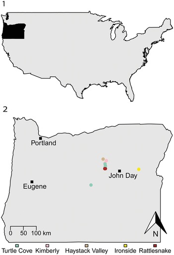
JDFB was selected as the study area because of its extensive Cenozoic time range spanning from the late Eocene through late Miocene, ~ 40 Myr. JDFB also has exceptional preservation of paleontological material. Geologic formations within the monument that contained previously collected castorid material include the John Day, Mascall, Ironside, and Rattlesnake formations (Fig. 1).
Localities of JDFB castorid specimens included in the analysis. (1) The contiguous USA with the state of Oregon in black. (2) Oregon with localities and geologic formation (or member units) noted by colored circles (see Supplementary Data for list of locality names and associated specimens). Black square = John Day, Oregon, USA: 44.415936°, -118.953995°.

Figure 1. Long description
A two-panel map layout.
Panel 1: A map of the contiguous United States in light gray. The state of Oregon, located in the Northwest, is highlighted in solid black.
Panel 2: A detailed map of Oregon.
* Major cities are marked with black squares: Portland in the Northwest and Eugene in the West-Central region.
* Fossil localities are concentrated in Central and Eastern Oregon, marked by colored circles.
* A cluster of localities is situated West of John Day, including Turtle Cove (light green), Kimberly (pink), Haystack Valley (tan), and Rattlesnake (dark red).
* A single yellow circle for Ironside is located East of John Day.
* A lone light green circle is located Southwest of the main cluster.
* A scale bar in the bottom-left indicates 0 to 100 kilometers.
* A North arrow is in the bottom-right corner.
* A legend at the bottom associates colors with geologic units: Turtle Cove, Kimberly, Haystack Valley, Ironside, and Rattlesnake.
The John Day Formation is currently subdivided into seven members: Big Basin (39.673–32.150 Ma), Turtle Cove (32.150–26.579 Ma), Kimberly (26.579–25.486 Ma), Haystack Valley (24.199–23.173 Ma), Balm Creek (23.173–22.466 Ma), Johnson Canyon (22.466–21.687 Ma), and Rose Creek (18.467–17.999 Ma) (Retallack et al., Reference Retallack, Bestland and Fremd2000; Hunt and Stepleton, Reference Hunt and Stepleton2004; Albright et al., Reference Albright, Woodburne, Fremd, Swisher, MacFadden and Scott2008; Mohr et al., Reference Mohr, Famoso, Samuels, Laib and Schmitz2025). The Big Basin Member is subdivided into three informal units, the lower (39.673–37.754 Ma; Eocene; Bartonian Stage/Age), middle (33.198–32.992 Ma; Oligocene; Orellen North American Land Mammal Age [NALMA]; Rupelian Stage/Age), and upper (32.992–32.15 Ma; Oligocene; Orellen NALMA; Rupelian Stage/Age) (Bestland and Retallack, Reference Bestland and Retallack1994; Mohr et al., Reference Mohr, Famoso, Samuels, Laib and Schmitz2025). The Turtle Cove and Kimberly consist of ~500 m of section that Albright et al. (Reference Albright, Woodburne, Fremd, Swisher, MacFadden and Scott2008) divided into 16 lithostratigraphic subunits (A–M) within the area near the Sheep Rock Unit of John Day Fossil Beds National Monument. These units are not laterally continuous in other areas where the Turtle Cove Member is exposed (e.g., Painted Hills Unit, Crooked River Basin). Included within the Turtle Cove Member are several dated tuffs and the Picture Gorge ignimbrite (PGI)—a supervolcanic event related to the Yellowstone hotspot (Seligman et al., Reference Seligman, Bindman, McClaughry, Stern and Fisher2014). The faunas of the Turtle Cove Member are assigned to the Whitneyan and Arikareean NALMAs (Oligocene; Rupelian Stage/Age) whereas the fauna of the Kimberly Member is assigned only to the Arikareean NALMA (Oligocene; Chattian Stage/Age) (Albright et al., Reference Albright, Woodburne, Fremd, Swisher, MacFadden and Scott2008). The Haystack Valley (Arikareean NALMA; Oligocene; Chattian Stage/Age), Balm Creek (Arikareean NALMA; Miocene; Aquitanian Stage/Age), Johnson Canyon (Arikareean NALMA; Miocene; Aquitanian Stage/Age), and Rose Creek (Hemingfordian NALMA; Miocene, Burdigalian Stage/Age) members were once all assigned to the Haystack Valley Member, but were split apart (Hunt and Stepleton, Reference Hunt and Stepleton2004).
Turtle Cove Member is composed of zeolitized blue-green claystone and welded tuffs representing a floodplain (Albright et al., Reference Albright, Woodburne, Fremd, Swisher, MacFadden and Scott2008). It is further broken down into separate units (A–D, E1–3, F–J, K1–2) and punctuated by several prominent tuff beds and the Picture Gorge Ignimbrite. Kimberly Member is composed of pinkish gray unzeolitized, tuffaceous siltstones, sandstones and conglomerates representing a floodplain (Hunt & Stapleton, Reference Hunt and Stepleton2004). It is further broken down into two separate units (L and M). Palaeocastor and Capacikala, the fossorial beavers, are found within both the Turtle Cove and Kimberly Members (Korth and Samuels, Reference Korth and Samuels2015). The semiaquatic beaver Microtheriomys is present in the Turtle Cove Member (Korth and Samuels, Reference Korth and Samuels2015).
The Mascall Formation is composed of alluvial siltstones, claystones, and tuffs representing a low relief fluvial drainage basin (Bestland et al., Reference Bestland, Forbes, Krull, Retallack and Fremd2008). It is primarily sampled in and around the Sheep Rock Unit of John Day Fossil Beds National Monument (Maguire et al., Reference Maguire, Samuels and Schmitz2018) and in the Crooked River Basin (McLaughlin et al., Reference McLaughlin, Hopkins and Schmitz2016; Barrett et al., Reference Barrett, Finkelman, Perdue, McLaughlin, Reuter and Hopkins2020). The Crooked River Mascall is between the ‘Double Tuff’ (16.44 ± 0.05 Ma) and the ‘Hawk Rim Tuff’ (16.260 ± 0.016 Ma) (McLaughlin et al., Reference McLaughlin, Hopkins and Schmitz2016), whereas the exposures around the Sheep Rock Unit are bound by the Dayville Basalt of the Picture Gorge Basalt Subgroup and the Rattlesnake Formation. Paleomagnetic analysis and radiometric dating placed the Dayville Basalt between 16.5 and 16.3 Ma (Long and Duncan, Reference Long and Duncan1982; Hooper and Swanson, Reference Hooper, Swanson and Walker1990; Maguire et al., Reference Maguire, Samuels and Schmitz2018). There are two dated ashes within the Mascall Formation, the ‘Mascall Tuff Bed’ (15.122 ± 0.017 Ma) and the ‘Kangaroo Tuff Bed’ (13.564 ± 0.018 Ma) (Maguire et al., Reference Maguire, Samuels and Schmitz2018). The Crooked River Mascall is assigned to the Hemingfordian NALMA (Miocene; Burdigalian Stage/Age), whereas the Mascall near the Sheep Rock Unit is assigned to the Barstovian NALMA (Miocene; Burdigalian and Langhian Stage/Age). The Mascall Formation around Sheep Rock Unit is subdivided into three informal units: the lower, middle, and upper. The semiaquatic beaver Monosaulax is present within the Mascall Formation.
The Ironside Formation is considered to be equivalent to the Juntura Formation and is assigned to the late Miocene Clarendonian NALMA (Serravallian and Tortonian Stage/Age) (Retallack, Reference Retallack2004, Reference Retallack2009). It consists of conglomerates, siltstones, lignites, and diatomites, and includes six pedotypes of paleosols (Retallack, Reference Retallack2004). The paleosols suggest a mixture of grasslands, woodlands, swamps, and riparian woodlands, which is also supported by the paleobotanical and vertebrate paleontological records. There is a gray volcanic ash in the Ironside Formation at the locality that our specimens came from; it is mineralogically most like the 11.31 Ma CPTXI Ash of the Great Basin (Perkins et al., Reference Perkins, Brown, Nash, McIntosh and Williams1998) and another gray tuff at the site is most like the 11.59 Ma CPTIX Ash (Retallack, Reference Retallack2004).
The Rattlesnake Formation is comprised of fluvial deposits, including conglomerates, siltstones, and sandstones (Enlows, Reference Enlows1976; J.E. Martin, Reference Martin1996; J.E. Martin and Fremd, Reference Martin and Fremd2001; Samuels and Zancanella, Reference Samuels and Zancanella2011) and includes a prominent volcanic ash layer, the Rattlesnake Ash Flow Tuff (RAFT), which has been 40Ar/39Ar dated to 7.05 ± 0.01 Ma (Streck and Grunder, Reference Streck and Grunder1995). Additionally, there is an undated white vitric tuff (‘Ted’s Tuff’), which forms a marker bed within the lower Rattlesnake Formation ~ 16.5 m above the base of the section (Retallack, Reference Retallack1999; Retallack et al., Reference Retallack, Tanaka and Tate2002). The Rattlesnake Formation is assigned to the late Miocene Hemphillian NALMA (Tortonian and Messinian Stage/Age). The semiaquatic beaver Dipoides is present within the Mascall, Ironside, and Rattlesnake formations (Wilson, Reference Wilson1934; Stirton, Reference Stirton1935) and the earliest record of the genus Castor in North America occurs in the Rattlesnake formation (Samuels and Zancanella, Reference Samuels and Zancanella2011).
Materials and methods
Specimens were selected based on dental material of fossorial (Palaeocastorinae) and semiaquatic (Anchitheriomyinae, Castorinae, and Castoroidinae) specimens available from JDFB collections. A total of 42 fossil beaver specimens containing 80 teeth from six genera Capacikala (N = 11 teeth), Castor (N = 2 teeth), Dipoides (N = 19 teeth), Microtheriomys (N = 6 teeth), Monosaulax (N = 4 teeth), and Palaeocastor (N = 38 teeth) were selected for the analysis. One extant specimen of Castor canadensis Kuhl, Reference Kuhl1820 from Oregon (UCLA 17854; N = 4 teeth) was included in the analysis. Scaled TIF photographs of JDFB specimens were taken of the occlusal surfaces of the teeth using a Nikon D810 camera and Dino-Eye AM7023CT 5MP C-mount microscope camera.
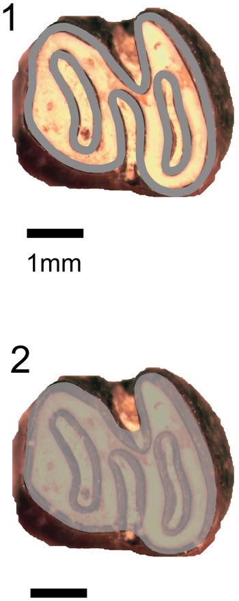
Occlusal Enamel Index (OEI) is calculated by the total lengths of enamel bands on the occlusal surface (Occlusal Enamel Length; OEL) divided by the square root of the tooth occlusal area (True Area) (Famoso et al., Reference Famoso, Feranec and Davis2013). OEL and True Area were traced and measured using ImageJ (version 1.53k) (Schneider et al., Reference Schneider, Rasband and Eliceiri2012) on a Fujitsu Lifebook T902 laptop/tablet (Fig. 2).
Areas used to calculate occlusal enamel index (OEI) on JODA 15132 Monosaulax sp. indet. (1) Enamel bands outlined to exclude areas composed of dentine, which are added together for a single tooth sum OEL value. (2) Total area of occlusal surface including both enamel and dentine.

Statistical analyses were completed using R Statistics program (version 4.5.2) (R Core Team, 2018). OEI values were tested for normality using the Shaprio-Wilk test. Data were not normally distributed, and analyses were run using nonparametric tests to avoid violation of any assumptions of parametric statistical tests.
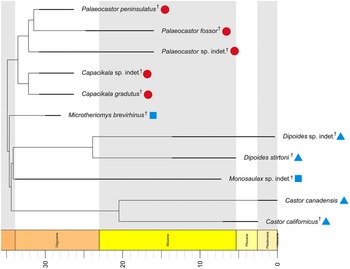
To test for phylogenetic signal within the dataset, an informal supertree of the six genera in the analysis were constructed using the Mesquite system for phylogenetic computing (Maddison and Maddison, Reference Maddison and Maddison2019). Placement of taxa on the tree were reasoned from consensus among previously published phylogenies (Martin, Reference Martin, Martin and Ostrander1987; Rybczynski, Reference Rybczynski2007, Reference Rybczynski2008; Samuels and Van Valkenburgh, Reference Samuels and Van Valkenburg2008, Reference Samuels and Van Valkenburgh2009; Calede, Reference Calede2014, Reference Calede2022; Korth and Samuels, Reference Korth and Samuels2015; Martin and Johnson, Reference Martin and Johnson2016; Plint et al., Reference Plint, Longstaffe, Ballantyne, Telka and Rybczynski2020). The phylogenetic supertree was time calibrated in R using the paleotree package (version 3.4.7; Bapst, Reference Bapst2012). First and last occurrence dates for each taxon were obtained through the Paleobiology Database (PBDB; Paleobiology Database, 2025) and added to the supertree to modify branch lengths (Supplementary Data; Fig. 3). The time calibrated supertree was run with OEI averages for each taxon to determine phylogenetic signal using the physignal function in the geomorph package (version 4.0.10) in R (Adams and Otárola-Castillo, Reference Adams and Otárola-Castillo2013).
Phylogenetic supertree of JDFB beaver taxa used in the analysis. Darker lines overlying branches represent the first and last occurrence of taxa in millions of years (taxa first and last occurrences listed in Supplementary Data). Species not otherwise discussed in the text are Dipoides stirtoni Wilson, Reference Wilson1934 and Microtheriomys brevirhinus Korth and Samuels, Reference Korth and Samuels2015. † = extinct taxon; blue square = nonwoodcutting, semiaquatic taxon; blue triangle = woodcutting, semiaquatic taxon; red circle = fossorial taxon.

Figure 3. Long description
A phylogenetic tree with a horizontal x-axis representing time in millions of years. The axis is divided into colored geological epochs: Oligocene in orange, Miocene in yellow, and Pliocene, Pleistocene, and Holocene in light green.
At the top, a clade of fossorial taxa marked with red circles includes Palaeocastor peninsulatus, Palaeocastor fossor, Palaeocastor species indet., Capacikala species indet., and Capacikala gradutus. Their temporal ranges, indicated by thick black lines, are concentrated between 30 and 20 million years ago.
In the middle, Microtheriomys brevirhinus is marked with a blue square, indicating a semiaquatic non-woodcutting lifestyle, appearing around 30 million years ago.
The lower half of the tree contains woodcutting semiaquatic taxa marked with blue triangles and additional semiaquatic taxa with blue squares. These include Dipoides species indet., Dipoides stirtoni, Monosaulax species indet., Castor canadensis, and Castor californicus. Their ranges extend from the Miocene through to the present day.
All taxa except Castor canadensis are marked with a dagger symbol indicating they are extinct. The branching structure shows the evolutionary relationships and divergence points between these groups relative to the geological timeline.
Because there was no phylogenetic signal present within the dataset, nonparametric statistical tests were run without including phylogeny. The residual randomization permutation procedure package (RRPP; version 2.1.2) in R was selected due to its ability to handle small datasets without relying on distributional assumptions of normality (Collyer and Adams, Reference Collyer and Adams2018, Reference Collyer and Adams2025). Linear models were created using the lm.rrpp function with OEI as the dependent variable and genus (Capacikala, Castor, Dipoides, Microtheriomys, Monosaulax, and Palaeocastor; N = 6), taxon (species)—e.g., Dipoides sp. indet., Capacikala gradatus (Cope, Reference Cope1879); N = 11—tooth position (p4, P4, M1, m2, etc.; N = 11), epoch (Oligocene, Miocene, and Holocene; N = 3), geologic formation (John Day, Mascall, Ironside, and Rattlesnake formations; N = 5), geologic formations with separated members of the John Day Formation (Turtle Cove A–F, G–K2; Kimberly L, M; N = 15), geologic formation with combined geologic units of the John Day Formation, ecology (semiaquatic and fossorial; N = 2), and ecology with semiaquatic split between woodcutting and nonwoodcutting taxa (N = 3) as independent variables (Supplementary Data). Combined geologic units of the John Day Formation were categorized as either ‘lower’ or ‘upper’ units. Lower units were designated as units of the Turtle Cove Member (A–F) until the PGI, whereas upper units were designated as units of the Turtle Cove (G–K2) and Kimberly Members (L and M) above the PGI. This divide between the upper and lower units at the PGI is due to faunal and habitat differences occurring within the John Day Formation pre- and postvolcanic activity at the PGI (Famoso et al., Reference Famoso, Samuels, Hopkins, Emery and Davis2015; Famoso, Reference Famoso2017; Reuter et al., Reference Reuter, Wainwright, Hoffman, Clementz, Blumenthal and Hopkins2025). Ecology was not analyzed as an independent variable as the phylogenetic supertree already incorporates ecological data into creating its topology. As such, incorporating ecology into the analysis would introduce circular reasoning. Fossorial beavers are restricted to within the subfamily Palaeocastorinae (which include Capacikala and Palaeocastor) whereas the other branches of the phylogenetic supertree are comprised of semiaquatic beaver taxa belonging to the subfamilies Anchitheriomyinae, Castorinae, and Castoroidinae (Castor, Dipoides, Microtheriomys, and Monosaulax).
Five hundred and eleven iterations of models were compared to evaluate various interactions between variables and to identify the optimal models to use for the analysis, which was done using the model.comparison function in the RRPP package. We used the log-likelihood model to produce Akaike Information Criterion (AIC) scores, which indicates the models with the best relative fit to the data, and is also robust to over fitting (Collyer and Adams, Reference Collyer and Adams2018, Reference Collyer and Adams2025). One RRPP linear model with all variables included and four optimized RRPP linear models were ultimately selected based on best fit determined by low AIC scores (Supplementary Data) and run through an analysis of variance (ANOVA) with ordinary least squares for coefficient estimation to test for any differences between group means and type III sum of squares to measure the individual contribution of each factor regardless of input order into the model. Posthoc pairwise comparison tests were run using the pairwise function in the RRPP package to test for differences between least-square means groups (similar to Tukey’s HSD). With the model.comparision function, we used the likelihood model to produce the AICs, which is also robust to over fitting (Collyer and Adams, Reference Collyer and Adams2018, Reference Collyer and Adams2025). Posthoc pairwise tests were run on variables with significant p-values resulting from the LM RRPP ANOVAs.
Repositories and institutional abbreviations
Fossil specimens examined in this study are reposited at John Day Fossil Beds National Monument (JODA), Kimberly, Oregon, USA. One modern specimen of Castor canadensis is reposited at the University of California Los Angeles (UCLA), Los Angeles, California, USA.
Results
Shapiro-Wilks normality test of OEI values resulted in non-normally distributed data (W = 0.91, p = 1.33 e-05). The test for phylogenetic signal resulted in no signal within the dataset for OEI values (K = 0, p = 0.056).
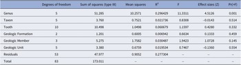
In the full RRPP linear model analysis of variance (RRPP LM ANOVA), which tested all variables, some of the variables were truncated due to redundancies within the dataset (e.g., removal of epoch and locomotor ecology; Table 1). Only genus (p = 0.001) was significant from the full model RRPP LM ANOVA (Table 1). Taxon (p = 0.514), tooth placement (tooth; p = 0.332), geologic formation (p = 0.459), combined upper and lower geologic units of the John Day Formation (geologic member; p = 0.145), and separated geologic members of the John Day Formation (geologic unit; p = 0.554) were not significant (Table 1). Four optimized models (with the lowest AIC scores of 245.55) were also tested in the RRPP LM ANOVA, and resulted in significant p-values for ecology, epoch, geologic formation, and geologic formations with combined upper and lower units of the Turtle Cove and Kimberly members of the John Day Formation (geologic member) (Tables 2–5).
Results of residual randomization permutation procedure linear model analysis of variance (RRPP LM ANOVA) of OEI values against genus, taxon, tooth position, epoch, geologic formation, geologic formation with combined geologic units of the John Day Formation (geologic member), geologic formations with separated members of the John Day Formation (geologic unit), and ecology. Epoch and ecology were truncated within the analysis, and so results are not present within the table. F = f-statistic; Pr(>F) = p-value; R2 = coefficient of determination

Table 1. Long description
The table consists of 8 columns: Degrees of freedom, Sum of squares (type III), Mean squares, R super 2, F, Effect sizes (Z), and Pr(>F).
* Genus: 5 degrees of freedom, Sum of squares 51.285, Mean squares 10.2571, R super 2 0.296429, F 11.3311, Z 4.5126, p-value 0.001.
* Taxon: 5 degrees of freedom, Sum of squares 3.760, Mean squares 0.7521, R super 2 0.021736, F 0.8308, Z minus 0.0143, p-value 0.514.
* Tooth: 10 degrees of freedom, Sum of squares 10.498, Mean squares 1.0498, R super 2 0.060679, F 1.1597, Z 0.4280, p-value 0.332.
* Geologic Formation: 2 degrees of freedom, Sum of squares 1.201, Mean squares 0.6005, R super 2 0.006942, F 0.6634, Z 0.1333, p-value 0.459.
* Geologic Member: 3 degrees of freedom, Sum of squares 5.275, Mean squares 1.7582, R super 2 0.030487, F 1.9423, Z 1.0728, p-value 0.145.
* Geologic Unit: 5 degrees of freedom, Sum of squares 3.380, Mean squares 0.6759, R super 2 0.019534, F 0.7467, Z minus 0.1360, p-value 0.554.
* Residuals: 53 degrees of freedom, Sum of squares 47.977, Mean squares 0.9052, R super 2 0.277304.
* Total: 83 degrees of freedom, Sum of squares 173.011.
Results of residual randomization permutation procedure linear model analysis of variance (RRPP LM ANOVA) of OEI values against geologic formation with combined geologic units of the John Day Formation (geologic member) and ecology. F = f-statistic; Pr(>F) = p-value; R2 = coefficient of determination

Table 2. Long description
The table consists of eight columns: Variable, Degrees of freedom, Sum of squares (type III), Mean squares, R super 2, F, Effect sizes (Z), and Pr(>F).
* Geologic Member: 7 degrees of freedom, sum of squares 93.432, mean squares 13.347, R super 2 0.54003, F 13.884, effect size 6.0443, and p-value 0.001.
* Ecology: 1 degree of freedom, sum of squares 62.992, mean squares 62.992, R super 2 0.36409, F 65.525, effect size 4.7624, and p-value 0.001.
* Residuals: 75 degrees of freedom, sum of squares 72.101, mean squares 0.961, and R super 2 0.41674. F, effect size, and p-value are not applicable.
* Total: 83 degrees of freedom and a total sum of squares of 173.011.
Results of residual randomization permutation procedure linear model analysis of variance (RRPP LM ANOVA) of OEI values against epoch, geologic formation with combined geologic units of the John Day Formation (geologic member), and ecology. F = f-statistic; Pr(>F) = p-value; R2 = coefficient of determination

Table 3. Long description
The table consists of eight columns: Variable, Degrees of freedom, Sum of squares, Mean squares, R super 2, F, Effect sizes (Z), and Pr(>F).
* Epoch: 2 degrees of freedom, sum of squares 14.001, mean squares 7.000, R super 2 0.08092, F 7.2819, Z 2.6560, p-value 0.004.
* Geologic Member: 5 degrees of freedom, sum of squares 27.052, mean squares 5.410, R super 2 0.15636, F 5.6280, Z 3.5038, p-value 0.001.
* Ecology: 1 degree of freedom, sum of squares 62.992, mean squares 62.992, R super 2 0.36409, F 65.5252, Z 4.7624, p-value 0.001.
* Residuals: 75 degrees of freedom, sum of squares 72.101, mean squares 0.961, R super 2 0.41674. F, Z, and p-value are not applicable.
* Total: 83 degrees of freedom, sum of squares 173.011. Other columns are not applicable.
Results of residual randomization permutation procedure linear model analysis of variance (RRPP LM ANOVA) of OEI values against geologic formation, geologic formation with combined geologic units of the John Day Formation (geologic member), and ecology. F = f-statistic; Pr(>F) = p-value; R2 = coefficient of determination

Table 4. Long description
The table consists of eight columns: Category, Degrees of freedom, Sum of squares, Mean squares, R super 2, F, Effect sizes (Z), and Pr(>F).
* Geologic Formation: 4 degrees of freedom, sum of squares 54.533, mean squares 13.633, R super 2 0.31520, F 14.1816, effect size 5.0314, and p-value 0.001.
* Geologic Member: 3 degrees of freedom, sum of squares 24.525, mean squares 8.175, R super 2 0.14175, F 8.5038, effect size 3.6329, and p-value 0.001.
* Ecology: 1 degree of freedom, sum of squares 62.992, mean squares 62.992, R super 2 0.36409, F 65.5252, effect size 4.7624, and p-value 0.001.
* Residuals: 75 degrees of freedom, sum of squares 72.101, mean squares 0.961, R super 2 0.41674. F, effect size, and p-value are not applicable.
* Total: 83 degrees of freedom, sum of squares 173.011. Other values are not applicable.
Results of residual randomization permutation procedure linear model analysis of variance (RRPP LM ANOVA) of OEI values against epoch, geologic formation, geologic formation with combined geologic units of the John Day Formation (geologic member), and ecology. F = f-statistic; Pr(>F) = p-value; R2 = coefficient of determination

Table 5. Long description
The table consists of 8 columns and 6 rows of data. The columns are labeled: Degrees of freedom, Sum of squares, Mean squares, R super 2, F, Effect sizes (Z), and Pr(>F).
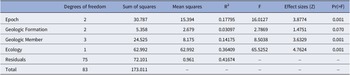
* Epoch: 2 degrees of freedom, sum of squares 30.787, mean squares 15.394, R super 2 0.17795, F 16.0127, Z 3.8774, p-value 0.001.
* Geologic Formation: 2 degrees of freedom, sum of squares 5.358, mean squares 2.679, R super 2 0.03097, F 2.7869, Z 1.4751, p-value 0.070.
* Geologic Member: 3 degrees of freedom, sum of squares 24.525, mean squares 8.175, R super 2 0.14175, F 8.5038, Z 3.6329, p-value 0.001.
* Ecology: 1 degree of freedom, sum of squares 62.992, mean squares 62.992, R super 2 0.36409, F 65.5252, Z 4.7624, p-value 0.001.
* Residuals: 75 degrees of freedom, sum of squares 72.101, mean squares 0.961, R super 2 0.41674.
* Total: 83 degrees of freedom, sum of squares 173.011.
Post-hoc pairwise comparison tests were run for genus, ecology, epoch, geologic formation, and geologic member; however, none of the variables resulted in any statistically significant differences between groups (Supplementary Data).
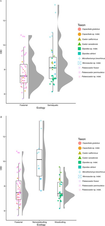
Mean OEI values tended to be slightly lower in general for fossorial taxa (mean = 7.81) than semiaquatic taxa (mean = 8.42) (Fig. 4.1). When separated between woodcutting and nonwoodcutting semiaquatic beavers, nonwoodcutting semiaquatic taxa had higher mean OEI values (mean = 10.23) than fossorial (mean = 7.81) and woodcutting semiaquatic taxa (mean = 7.69) (Fig. 4.2).
Raincloud plots of OEI values for ecologies of JDFB castorid taxa. (1) For fossorial and semiaquatic taxa. (2) For fossorial, nonwoodcutting semiaquatic, and woodcutting semiaquatic JDFB castorid taxa (see next page).

Figure 4. Long description
Two vertically stacked raincloud plots. Both plots use a Y axis labeled O E I ranging from 6 to 12 and an X axis labeled Ecology.
Panel 1 compares two groups:
* Fossorial: A box plot centered around 7.5 with jittered pink star and orange circle points. A grey density curve to the right shows a primary peak near 7.5 and a secondary peak near 9.5.
* Semiaquatic: A box plot centered around 8.2 with jittered blue cross, green triangle, and teal square points. The density curve shows a broad distribution with a peak around 7.5 and a smaller peak near 10.5.
Panel 2 compares three groups:
* Fossorial: Identical to Panel 1.
* Nonwoodcutting: A box plot centered higher, around 10.2, with blue cross and blue square points. The density curve is elongated with a peak near 10.
* Woodcutting: A box plot centered around 7.5 with green triangle and teal square points. The density curve is concentrated with a sharp peak near 7.2.
A shared legend to the right identifies taxa including Capacikala, Castor, Dipoides, Microtheriomys, Monosaulax, and Palaeocastor using distinct colors and symbols like circles, triangles, squares, crosses, and stars.
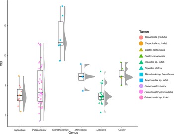
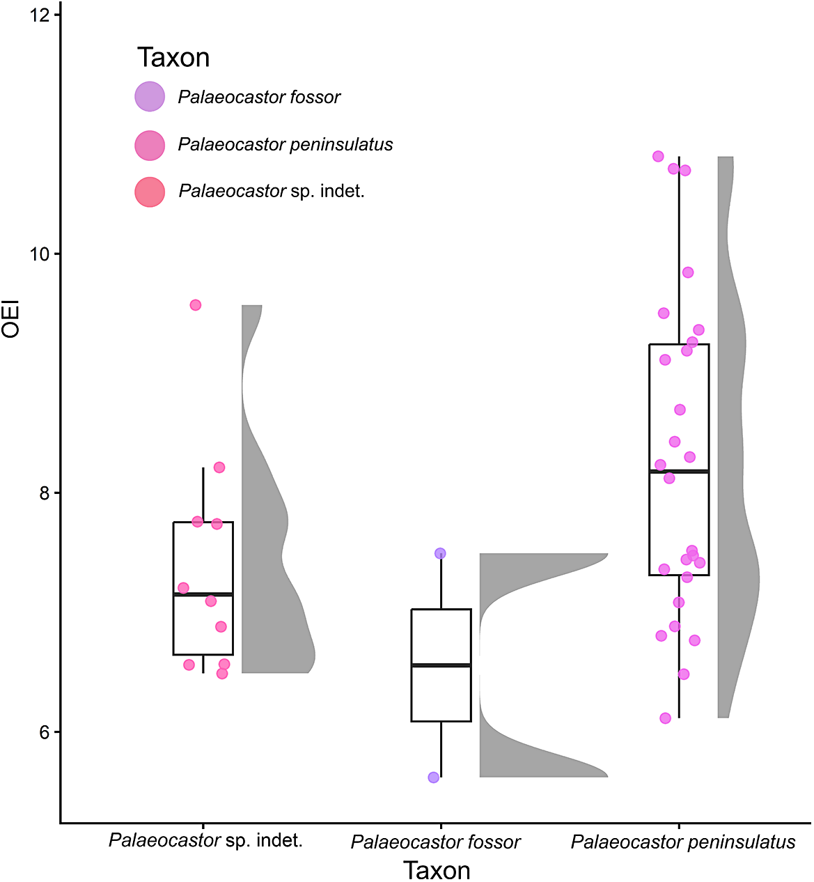
Microtheriomys displayed the highest average OEI values (mean = 11.34) compared to the other semiaquatic beavers included in the analysis (Castor, Dipoides, and Monosaulax) (Fig. 5). Monosaulax (mean = 8.56) and Castor (mean = 8.71) had higher average OEI values than Dipoides (mean = 7.37) (Fig. 5). Palaeocastor had the highest OEI values of the fossorial beavers (mean = 7.95) (Figs. 4, 5). The average OEI values of Capacikala (mean = 7.34) were lower than those of Palaeocastor (Figs. 4, 5), and between Palaeocastor species, P. fossor had the lowest average OEI values (mean = 6.56) (Fig. 6).
Raincloud plot of OEI values of JDFB castorid genera. Symbology denotes ecology, with circles representing fossorial taxa, squares nonwoodcutting semiaquatic taxa, and triangles woodcutting semiaquatic taxa.

Figure 5. Long description
A raincloud plot with the Y-axis representing O E I values from 6 to 12 and the X-axis listing six genera. Each genus entry consists of a vertical jittered dot plot on the left, a box plot in the center, and a grey density distribution curve on the right.
* Capacikala: Fossorial taxa represented by pink and orange circles. O E I values range from approximately 6.2 to 8.6 with a median near 7.4.
* Palaeocastor: Fossorial taxa represented by purple and pink circles. This group shows a wide vertical spread from 5.6 to 10.8 with a median near 7.5.
* Microtheriomys: Nonwoodcutting semiaquatic taxa represented by light blue squares. Values are high, ranging from 9.6 to 13.2 with a median near 10.8.
* Monosaulax: Nonwoodcutting semiaquatic taxa represented by blue squares. Values cluster between 7.6 and 9.4 with a median near 8.6.
* Dipoides: Woodcutting semiaquatic taxa represented by green and teal triangles. Values range from 6.2 to 9.0 with a median near 7.3.
* Castor: Woodcutting semiaquatic taxa represented by olive and green triangles. Values cluster tightly between 8.0 and 9.6 with a median near 8.6.
A Taxon legend on the right identifies specific species including Capacikala gradutus, Castor canadensis, and Palaeocastor fossor among others.
Raincloud plot of OEI of JDFB Palaeocastor spp.

Figure 6. Long description
The vertical y-axis is labeled O E I with a scale from 6 to 12. The horizontal x-axis is labeled Taxon. A legend at the top left identifies three species by color: Palaeocastor fossor in light purple, Palaeocastor peninsulatus in medium pink, and Palaeocastor sp. indet. in bright pink.
Each taxon is represented by a raincloud plot consisting of a jittered raw data point cloud, a box plot, and a vertical density distribution half-violin.
1. Palaeocastor sp. indet. (Left): The data is centered around an O E I of 7. The box plot shows a median near 7.2, with whiskers extending from approximately 6.5 to 8.2. One outlier is visible near 9.5.
2. Palaeocastor fossor (Center): This group has the lowest values, with a median near 6.5. The box plot is compact, ranging from 6 to 7. The density plot shows a sharp peak at the median.
3. Palaeocastor peninsulatus (Right): This group has the highest and most varied values. The median is approximately 8.2. The box plot spans from 7.5 to 9.2, with whiskers reaching from 6 to 11. The density plot is elongated, indicating a broad distribution of O E I values.
Discussion
Lifestyles in castorids are inherently tied to taxonomy because fossorial beavers are restricted to within the subfamily Palaeocastorinae whereas semiaquatic beavers from JDFB are represented in the subfamilies Anchitheriomyinae, Castorinae, and Castoroidinae (Korth, Reference Korth2001; Rybczynski, Reference Rybczynski2007, Reference Rybczynski2008; Calede, Reference Calede2014, Reference Calede2022). Within our analysis, the fossorial Palaeocastorine beavers include the genera Capacikala and Palaeocastor, whereas semiaquatic beavers are comprised of Microtheriomys in Anchitheriomyinae, Monosaulax and Dipoides in Castoroidinae, and Castor in Castorinae (Fig. 3).
Although genus, ecology, epoch, geologic formation, and geologic member appeared significant within the RRPP analysis, it is likely that they were not significant within the posthoc tests due to similarities and dependencies between some variable categories. Fossorial beavers all cluster within the Oligocene-aged John Day Formation (Turtle Cove, Kimberly, and Haystack Valley members). All of the other semiaquatic beavers, except for Microtheriomys, all clustered in the Miocene-aged Mascall, Ironside, and Rattlesnake formations (or Holocene for extant Castor canadensis). Microtheriomys was the outlier for the semiaquatic beavers, being found in the John Day Formation (Turtle Cove Unit H; Oligocene).
The heightened OEC in Microtheriomys compared to the other semiaquatic beavers included in the analysis (Castor, Dipoides, and Monosaulax) could be attributed to Microtheriomys being the smallest of the semiaquatic beavers from JDFB (Calede, Reference Calede2022). Although it is unknown if Microtheriomys would engage in woodcutting behaviors (Calede, Reference Calede2022), the common ancestor of semiaquatic castorids is hypothesized to have consumed woody plants (Plint et al., Reference Plint, Longstaffe, Ballantyne, Telka and Rybczynski2020). Microtheriomys is placed within the subfamily Anchitheriomyinae based on shared morphological features within that group (including complexity of occlusal surface pattern), however it has been suggested that it might actually be part of Castorinae based on similarities between early members of that subfamily (Korth and Samuels, Reference Korth and Samuels2015). Further evaluation of its taxonomic placement could aid in the understanding of OEC and body size in castorids, especially between semiaquatic beavers.
Monosaulax is also among the smaller of the semiaquatic beavers (Calede, Reference Calede2022) from JDFB and is thought to be an ancestral member of the Eucastor/Dipiodes/Castoroides lineage (Stirton, Reference Stirton1935; Korth, Reference Korth1994, Reference Korth2001; May and Brown, Reference May and Brown2023). Decreased OEC between Monosaulax and Dipoides could correlate with the general trend of increased body size within that lineage (i.e., Castoroides Foster, Reference Foster1838).
Although both Castor and Dipoides share similarities as woodcutting beavers with Holarctic distributions, they are not closely related and belong to different subfamilies (Castor to Castorinae and Dipoides to Castoroidinae; Fig. 3; Rybczynski, Reference Rybczynski2007, Reference Rybczynski2008). Based on incisor shape and cutting efficiency, Castor is a more efficient woodcutter than Dipoides (Rybczynski, Reference Rybczynski2008). Differences in woodcutting behaviors between the two taxa suggest niche partitioning (Rybczynski, Reference Rybczynski2007, Reference Rybczynski2008), which is further supported by differences in diet (Plint et al., Reference Plint, Longstaffe, Ballantyne, Telka and Rybczynski2020). The diet of Castor was predominantly composed of equal parts woody and aquatic vegetation, whereas the diet of Dipoides was composed of woody plants but tended more toward consumption of aquatic vegetation (Plint et al., Reference Plint, Longstaffe, Ballantyne, Telka and Rybczynski2020). Castor has higher OEC and larger body size than Dipoides (Plint et al., Reference Plint, Longstaffe, Ballantyne, Telka and Rybczynski2020), suggesting that Castor was better adapted at processing more fibrous, woody vegetation than Dipoides due to increased chewing potential.
Morphological and ecological similarities between Castor californicus Kellogg, Reference Kellogg1911 and Castor canadensis reaffirm an anagenetic relationship over time as chronospecies (Lubbers and Samuels, Reference Lubbers and Samuels2023; Lubbers et al., Reference Lubbers, Samuels and Joyner2025). Therefore, it is perhaps not surprising that their OEI values overlap (Fig. 5).
Capacikala and Palaeocastor both belong to Palaeocastorinae and share many morphological similarities, indicating fossorial lifestyles (Stefen, Reference Stefen2014). Although specific digging behaviors (i.e., scratch, chisel, head-lift digging) have not been assessed for Capacikala, cranial and postcranial morphologies suggest that Capacikala was likely a less specialized burrower compared to other Palaeocastorine beavers (Calede et al., Reference Calede, Samuels and Chen2019; Scarpitti and Calede, Reference Scarpitti and Calede2021). Unlike Palaeocastor fossor, Capacikala species are not directly associated with Daemonelix burrowing structures (Stefen, Reference Stefen2014).
Differences in OEC between Palaeocastor fossor and P. peninsulatus (Cope, Reference Cope1881) could be attributed to niche partitioning from varying digging behaviors (Fig. 6). Cranial and dental morphology characterizes P. fossor as a chisel digger (i.e., digging with incisors), whereas P. peninsulatus was likely a scratch digger (i.e., digging with forelimbs) (Samuels and Van Valkenburgh, Reference Samuels and Van Valkenburgh2009; Calede, Reference Calede2014). Habitat preferences have been noted with differing digging styles, because chisel diggers generally prefer more consolidated soils whereas scratch diggers prefer softer soils (Nevo, Reference Nevo1999). Chisel diggers also tend to have more elongated, procumbent incisors, which can help reduce the amount of grit exposed to cheek teeth while digging (Calede, Reference Calede2014). In general, P. fossor is more adapted to fossorial lifestyles than P. peninsulatus (see Calede, Reference Calede2014).
The common ancestor of Castoridae was most likely fossorial, whereas the common ancestor of semiaquatic beavers (Anchitheriomyinae, Castorinae, and Castorodinae) was most likely semiaquatic (Calede, Reference Calede2022). Certain skeletal morphologies adapted for semiaquatic lifestyles can often overlap with those for fossorial lifestyles, so it is not surprising that early castorids likely co-opted these fossorial traits for semiaquatic lifestyles (Samuels and Van Valkenburgh, Reference Samuels and Van Valkenburg2008; Calede, Reference Calede2022).
Our results suggest that castorids did not rely on OEC to combat higher rates of wear from dental abrasion between fossorial and woodcutting semiaquatic taxa. Although not evaluated quantitatively here, we hypothesize that other factors (e.g., hypsodonty) might be a bigger factor. Previous studies comparing OEI and hypsodonty on ungulates showed that there was no evolutionary correlation between the two factors (Famoso et al., Reference Famoso, Feranec and Davis2013, Reference Famoso, Davis, Feranec, Hopkins and Price2016). Strategies to combat dental wear typically evolved to either increase hypsodonty or enamel complexity, not both (Famoso and Davis, Reference Famoso and Davis2016; Famoso et al., Reference Famoso, Davis, Feranec, Hopkins and Price2016). This adaptive response has been shown in Miocene horses, with Hipparionini horses having high OEC and lower crown heights, whereas Equini horses had lower OEC and higher crowned teeth (Famoso and Davis, Reference Famoso and Davis2014, Reference Famoso and Davis2016; Famoso et al., Reference Famoso, Davis, Feranec, Hopkins and Price2016). Other chisel-digging fossorial rodents, e.g., pocket gophers (Geomyidae), show similar adaptive responses by having simple, low OEC, and high-crowned teeth (Korth, Reference Korth1994; Samuels and Van Valkenburg, Reference Samuels and Van Valkenburgh2009). This suggests that the more advantageous adaptation to combat dental wear from abrasive grit in the substratum is higher-crowned teeth rather than increased enamel complexity. DeMiguel et al. (Reference DeMiguel, Azanza, Cegonino, Ruiz and Morales2016) found that hypsodont teeth reduce dental stress and increase shearing pressures, which aid in breaking down tough, fibrous vegetation (i.e., grasses, woody vegetation). This could explain why enamel complexity was lower in the woodcutting semiaquatic beavers compared to the nonwoodcutting taxa. Overall, it appears that hypsodont dentition was likely a more advantageous adaptation for combating abrasive dental wear from gritty substratum and fibrous, woody vegetation in both fossorial and woodcutting semiaquatic beaver taxa, whereas OEC was likely more helpful in increasing chewing potential, especially within the smaller, nonwoodcutting semiaquatic members of Castoridae (i.e., Microtheriomys).
Hypsodonty was not evaluated in this analysis due to varied crown heights over time in our taxonomic sample (i.e., mesodont [Monosaulax], subhypsodont [Capacikala and Palaeocastor], hypsodont [Castor and Microtheriomys], and hypselodont [Dipoides]), which, coupled with varying levels of wear on the JDFB specimens, made it difficult to calculate hypsodonty index. Sampling within the JDFB specimens would also be challenging because some specimens have teeth contained within maxillae and dentaries, which would make accessing the full crown height difficult without CT scanning the specimens or removing cortical bone.
In general, small herbivorous mammals need to maximize nutrient intake to sustain their higher base energy needs (Pineda-Munoz et al., Reference Pineda-Munoz, Evans and Alroy2016). One way to increase nutritional uptake is by increasing chewing potential to maximize chewing efficiency, which can be accomplished through increased OEC. Although we did not evaluate body mass as part of this work, body mass has been shown to correlate with tooth area in ungulates (Famoso et al., Reference Famoso, Feranec and Davis2013), because larger mammals can increase their chewing potential by increasing the occlusal surface area in size rather than relying on increased surface area from OEC (Pineda-Munoz et al., Reference Pineda-Munoz, Evans and Alroy2016). Larger mammals can also consume higher volumes of less nutrient-dense foods due to their lower energy needs and increased digestive processing capabilities from larger body size (Pineda-Munoz et al., Reference Pineda-Munoz, Evans and Alroy2016). Body size was not included in this analysis due to lack of postcrania or complete tooth rows associated with the specimens preserved at JDFB, which are often used as proxies for estimating body mass (e.g., Reynolds, Reference Reynolds2002; Hopkins, Reference Hopkins2008; Freudenthal and Martín-Suárez, Reference Freudenthal and Martín-Suárez2013). A further quantitative investigation into the relationship of body mass and OEC within castorids would be a useful metric for future studies to incorporate.
This study documents OEC on castorids from JDFB and serves as a starting point for further work. Although limited, it provides a first step for understanding dental adaptations in castorids. Future analysis should increase the specimen sample size to include other castorids, both of taxa already represented and from other localities outside (geographically and temporally) of JDFB, for better resolution and more robust results.
Conclusion
This study provides an initial assessment of enamel complexity in Castoridae from a regional locality and provides an analysis for the effects of differing ecologies on one component of adaptations to combating dental wear. Our results indicate that fossorial and woodcutting semiaquatic JDFB castorids are not relying on OEC to combat dental wear. Although limited in terms of sample size and geographic scope, this study provides a starting point for further evaluations on enamel complexity within Castoridae, especially of taxa inhabiting different ecologies. Future work should include additional taxa and sample size, in addition to comparing OEC with other metrics including body size and hypsodonty index to better understand the adaptive responses of beavers to differing ecologies and the general relationship with OEC in Castoridae.
Acknowledgments
This project was initiated while KEL was a Scientists in Parks intern in 2021. Support for this internship was provided by the National Park Service (NPS) and Conservation Legacy. We thank J. Cavin and C. Schierup at John Day Fossil Beds National Monument for their added assistance in facilitating this project, both in the field and collections. We thank the NPS and Bureau of Land Management (BLM) for access to collections from their administered lands. We thank three anonymous reviewers, editor E. Hermsen, and guest editor A. Kort for their helpful suggestions that greatly improved the manuscript.
Competing interests
The authors declare none.
Data availability statement
Supplementary Data are available from https://doi.org/10.5061/dryad.2z34tmq2g.




 Open access

